Non-Markovian effects in stochastic resonance in a two level system

Abstract

Stochastic resonance is a phenomenon where the response signal to external driving is enhanced by environment noise. In quantum regime, the effect of environment is often intrinsically non-Markovian. Due to the combination of such non-Markovian quantum noise and external driving force, it is difficult to evaluate the correlation function and hence the power spectrum. Nevertheless, a recently developed algorithm, which is called time-evolving matrix product operators (TEMPO), and its extensions provide an efficient and numerically exact approach for this task. Using TEMPO we investigate non-Markovian effects in quantum stochastic resonance in a two level system. The periodic signal and the time-averaged asymptotic correlation function, along with the power spectrum, are calculated. From the power spectrum the signal-to-noise ratio is evaluated. It is shown that both signal strength and signal-to-noise ratio are enhanced by non-Markovian effects, which indicates the importance of non-Markovian effects in quantum stochastic resonance. In addition, we show that the non-Markovian effects can shift the peak position of the background noise power spectrum.

I Introduction

Stochastic resonance (SR) is phenomenon for which the response of the system to external driving is enhanced by noise, which was first proposed by Benzi et al. Benzi et al. (1981). Since then SR has continuously attracted considerable attention over several decades. The first experimental verification of such phenomenon was obtained by Fauve and Heslot Fauve and Heslot (1983), who studied the noise-induced transition process in a bistable system. Another key experiment in this field is the observation of SR in an optical device, the bidirectional ring laser, by McNamara et al. McNamara et al. (1988). The concept of SR was extended to the quantum regime, which is referred as quantum stochastic resonance (QSR), by Löfstedt and Coppersmith Löfstedt and Coppersmith (1994) by measuring conductance fluctuations in mesoscopic metals. A control scheme for SR using a Schmitt trigger is demonstrated by Gammaitoni et al. Gammaitoni et al. (1999). Recently, QSR is demonstrated in the a.c.-driven charging and discharging of single electron on a quantum dot Wagner et al. (2019); Hussein et al. (2020) and in individual Fe atoms Hänze et al. (2021).

The theoretical investigation for SR in terms of periodically driven dissipative system starts several decades ago, and comprehensive reviews can be found in Refs. McNamara and Wiesenfeld (1989); Jung (1993); Grifoni and Hänggi (1998); Gammaitoni et al. (1998). When the quantum coherence is suppressed, both quantum and classical SR can be well described by the classical rate equation approach McNamara and Wiesenfeld (1989). In deep quantum regime, qualitative new features arise Grifoni et al. (1996); Grifoni and Hänggi (1996). This regime has been investigated semiclassically by Grifoni et al. Grifoni et al. (1996) and numerically by Makarov and Makri Makarov and Makri (1995a, b). The QSR in a system driven by weak signal and white noise was studied by Joshi Joshi (2008).

The non-Markovian transient property of QSR is difficult to evaluate due to the interplay of dissipative and external driving. A numerically exact method known as quasi-adiabatic propagator path integral (QUAPI) method Makarov and Makri (1995a, b), which fully takes the non-Markovian effects into consideration, is meant to be suitable for such task. However, the computational cost of QUAPI grows exponentially with size of the system Hilbert space and memory length, therefore although numerically exact, QUAPI can become highly inefficient or even infeasible under certain circumstances. Due to this limitation, the correlation function and the corresponding power spectrum, which is the quantity of fundamental interest in QSR study, are not suitable to be evaluated by bare QUAPI algorithm.

Recently, Strathearn et al. Strathearn et al. (2018) show that QUAPI method can be represented in the framework of matrix product states (MPS) Schollwöck (2011); Orús (2014). The standard MPS compression algorithm is applicable in this framework, and thus they obtain an efficient and numerically exact method which is called time-evolving matrix product operators (TEMPO). Later Jørgensen and Pollock Jørgensen and Pollock (2019) relate TEMPO to process tensor to motivate an efficient and numerically exact algorithm for simulation of correlation functions in undriven open systems. The TEMPO method is also modified for repeated computation of various sets of parameters by Fux et al. Fux et al. (2021).

In this article, we employ TEMPO to study the non-Markovian effects in QSR in an open two level system which is periodically driven. The periodic signal is evaluated for which the signal strength shows a maximum as noise level increases, which is a sign of QSR. In the Markovian limit, the signal almost vanishes, while the signal reappears when non-Markovian effects are included. The signal strength increases with increasing non-Markovianity, which shows that the non-Markovian effects plays an essential role in QSR.

The asymptotic correlation function are evaluated with different initial time. Unlike the periodic signal, whose strength increases with increasing non-Markovianity, the amplitude of asymptotic correlation function can remain very small with certain initial time. The Fourier transform of the time-averaged asymptotic correlation gives the power spectrum, from which the background noise power and signal-to-noise ratio (SNR) are obtained. The SNR is also enhanced by non-Markovian effects. The peak position of background noise power can be shifted by the non-Markovian effects, which makes that the maximum of signal strength and SNR appear at different noise levels.

This article is organized as follows. The introduction of the model and method are given in Sec. II and III, respectively. The non-Markovian effects on observable and correlation function are discussed in Sec. IV and V, respectively. Section VI gives the result of signal-to-noise ratio. Finally a conclusion is given in Sec. VII.

II Model

Bistable system is the simplest and also the most widely used model to study stochastic resonance. Such a bistable system can be effectively described by a two level system, when external driving is present the Hamiltonian can be written as

$$H_{\mathrm{S}}(t)=\frac{\Delta}{2}\sigma_{x}+\frac{E}{2}\sigma_{z}\cos\Omega t,$$ (1)

where $\sigma_{z}$ and $\sigma_{x}$ are Pauli matrices, and the eigenstates of $\sigma_{z}$ are the basis states in a localized representation. Here $\Delta$ gives the tunneling amplitude between two levels, $E$ is the strength of external driving and $\Omega$ is driving frequency.

Here we consider a Caldeira-Leggett type model Caldeira and Leggett (1983a, b) for which the bath Hamiltonian and the system-bath coupling are

$$H_{\mathrm{B}}=\sum_{k}\omega_{k}b_{k}^{{\dagger}}b_{k},\quad H_{\mathrm{SB}}=\sigma_{z}\sum_{k}V_{k}(b_{k}^{{\dagger}}+b),$$ (2)

where the operator $b_{k}^{{\dagger}}$ ($b_{k}$) creates (annihilates) a boson in state $k$ with frequency $\omega_{k}$. The total Hamiltonian is

$$H=H_{\mathrm{S}}(t)+H_{\mathrm{B}}+H_{\mathrm{SB}}.$$ (3)

This model is usually referred as spin-boson model Leggett et al. (1987); Weiss (1993). The bath is characterized by a spectral function $J(\omega)$ and in this article we choose Ohmic dissipation for which

$$J(\omega)=\lambda\omega e^{-\omega/\omega_{c}},$$ (4)

where $\lambda$ is the coupling strength parameter and $\omega_{c}$ is the cutoff frequency. If the bath is in thermal equilibrium state then the bath autocorrelation function is written in terms of $J(\omega)$ as

$$\alpha(t)=\int_{0}^{\infty}J(\omega)\quantity[\coth(\frac{\omega}{2T})\cos\omega t-i\sin\omega t]\differential{\omega},$$ (5)

where $T$ is the temperature. The noise level is determined by the coupling strength and the temperature. Throughout this article we set $\hbar=k_{B}=1$ and use dimensionless quantities.

The relevant theoretical quantity describing the dissipative dynamics is the expectation value of observable $\expectationvalue{\sigma_{z}(t)}$. Under periodic driving, this quantity shows coherent oscillations in steady state whose amplitude gives the periodic signal strength. The signal strength shows a maximum with respect to noise level Makarov and Makri (1995a, b), which is a sign of QSR.

Sometimes the correlation function is of more concern. The symmetrized correlation function is defined

$$C(t_{1},t_{2})=\frac{1}{2}\expectationvalue{\sigma_{z}(t_{1})\sigma_{z}(t_{2})+\sigma_{z}(t_{2})\sigma_{z}(t_{1})}.$$ (6)

Under this definition, the correlation function is symmetrized in the sense that $C(t_{1},t_{2})=C(t_{2},t_{1})$, and we can write

$$C(t_{1},t_{2})=\begin{cases}\real\expectationvalue{\sigma_{z}(t_{1})\sigma_{z}(t_{2})},&t_{2}\geq t_{1};\\ \real\expectationvalue{\sigma_{z}(t_{2})\sigma_{z}(t_{1})},&t_{1}\geq t_{2}.\\ \end{cases}$$ (7)

It means the symmetrized correlation function $C(t_{1},t_{2})$ is a real quantity and the knowledge of the correlation function $\expectationvalue{\sigma_{z}(t_{1})\sigma_{z}(t_{2})}$ for $t_{2}\geq t_{1}$ is enough to obtain whole $C(t_{1},t_{2})$. Therefore we focus on $C(t_{0},t_{0}+t)$ for $t\geq 0$ situation. The time-averaged, asymptotic (i.e., $t_{0}\to\infty$) symmetrized correlation function is defined as

$$\bar{C}(t)=\lim_{t_{0}\to\infty}\frac{\omega}{2\pi}\int_{0}^{\frac{2\pi}{\omega}}C(t_{0},t_{0}+t)\differential{t_{0}}.$$ (8)

The quantity of experimental interest for QSR is the power spectrum McNamara and Wiesenfeld (1989); Grifoni and Hänggi (1998), which is defined one-sided, i.e., for positive $\omega$ only, as

$$\begin{split}\bar{S}(\omega)&=\frac{1}{2}\int_{-\infty}^{\infty}\bar{C}(t)(e^{i\omega t}+e^{-i\omega t})\differential{t}\\ &=\int_{-\infty}^{\infty}\bar{C}(t)\cos\omega t\differential{t}.\end{split}$$ (9)

III Method

III.1 Quasi-Adiabatic Propagator Path Integral

Here we give a brief review of the QUAPI and TEMPO method. Let $\rho(t)$ denote the total density matrix, then the time evolution of $\rho$ is given by

$$\rho(t)=U(t,0)\rho(0)U^{{\dagger}}(t,0),$$ (10)

where

$$U(t,t_{0})=\mathrm{T}\exp[-i\int_{t_{0}}^{t}H(\tau)\differential{\tau}].$$ (11)

Here $\mathrm{T}$ denotes the chronological ordering operator. The reduced density matrix is defined as $\rho_{\mathrm{S}}(t)=\Tr_{\mathrm{B}}[\rho(t)]$, where $\Tr_{\mathrm{B}}$ denote the trace over the bath degrees of freedom. Let $s$ denote the eigenvalue of $\sigma_{z}$, then the element of the reduced density matrix can be written as

$$\rho_{\mathrm{S}}(s^{\prime\prime},s^{\prime};t)=\Tr_{\mathrm{B}}\matrixelement{s^{\prime\prime}}{U(t,0)\rho(0)U^{{\dagger}}(t,0)}{s^{\prime}}.$$ (12)

If at initial time $t=0$ the total density matrix is in product state for which

$$\rho(0)=\rho_{\mathrm{S}}(0)\otimes\rho_{\mathrm{B}},$$ (13)

then the above expression can be written in path integral form by splitting the evolution into $N$ pieces for which $\delta t=t/N$ with $N\to\infty$. Relabeling $s^{\prime\prime},s^{\prime}$ as $s_{N}^{+},s_{N}^{-}$ yields

$$\rho_{\mathrm{S}}(s_{N}^{\pm})=\sum_{s_{0}^{\pm},\ldots,s_{N-1}^{\pm}}F(s_{0}^{\pm},\ldots,s_{N}^{\pm}),$$ (14)

where $\rho_{\mathrm{S}}(s_{N}^{\pm})$ denotes $\matrixelement{s_{N}^{+}}{\rho_{\mathrm{S}}(t)}{s_{N}^{-}}$ and

$$F(s_{0}^{\pm},\ldots,s_{N}^{\pm})=K(s_{0}^{\pm},\ldots,s_{N}^{\pm})I(s_{0}^{\pm},\ldots,s_{N}^{\pm}).$$ (15)

Here $K(s_{0}^{\pm},\ldots,s_{N}^{\pm})$ is the bare system propagating tensor for which

$$K(s_{0}^{\pm},\ldots,s_{N}^{\pm})=\rho_{\mathrm{S}}(s_{0}^{\pm})\tilde{K}(s_{0}^{\pm},s_{1}^{\pm})\cdots\tilde{K}(s_{N-1}^{\pm},s_{N}^{\pm}),$$ (16)

where ($t_{k}=k\delta t$)

$$\begin{split}\tilde{K}(s_{k-1}^{\pm},s_{k}^{\pm})=&\matrixelement{s_{k}^{+}}{U(t_{k},t_{k-1})}{s_{k-1}^{+}}\\ &\times\matrixelement{s_{k-1}^{-}}{U^{{\dagger}}(t_{k},t_{k-1})}{s_{k}^{-}}.\end{split}$$ (17)

In the continuum limit $\delta t\to 0$, the collections of $(s_{0}^{+},\ldots,s_{N}^{+})$ and $(s_{0}^{-},\ldots,s_{N}^{-})$ can be regarded as a forward path $s^{+}(t^{\prime})$ and a backward path $s^{-}(t^{\prime})$ from 0 to $t$. If at initial time the bath is in thermal equilibrium state that $\rho_{\mathrm{B}}=e^{-H_{\mathrm{B}}/T}$, then the influence functional $I[s^{\pm}(t)]$ can be written as Feynman and Vernon (1963); Feynman and Hibbs (1965); Caldeira and Leggett (1983a)

$$e^{-\int_{0}^{t}\differential{t^{\prime}}\int_{0}^{t^{\prime}}\differential{t^{\prime\prime}}[s^{+}(t^{\prime})-s^{-}(t^{\prime})][\alpha(t^{\prime}-t^{\prime\prime})s^{+}(t^{\prime\prime})-\alpha^{*}(t^{\prime}-t^{\prime\prime})s^{-}(t^{\prime\prime})]},$$ (18)

where $\alpha(t)$ is the autocorrelation function given by (5). When employing finite $\delta t$ approximation, this influence functional can be discretized as

$$I(s_{0}^{\pm},\ldots,s_{N}^{\pm})=\exp[-\sum_{j=0}^{N}\sum_{k=0}^{j}\phi_{jk}],$$ (19)

where

$$\phi_{jk}=(s_{j}^{+}-s_{j}^{-})(\eta_{jk}s_{k}^{+}-\eta_{jk}^{*}s_{k}^{-}).$$ (20)

Here the form of $\eta_{jk}$ depends on choice of discretization scheme Dattani et al. (2012).

The discretized influence functional (19) is a tensor which can be decomposed as

$$\begin{split}I(s_{0}^{\pm},\ldots,s_{N}^{\pm})=&\prod_{k=0}^{N}I_{0}(s_{k}^{\pm},s_{k}^{\pm})\prod_{k=0}^{N-1}I_{1}(s_{k}^{\pm},s_{k+1}^{\pm})\cdots\\ &\times\prod_{k=0}^{N-\Delta k}I_{\Delta k}(s_{k}^{\pm},s_{k+\Delta k}^{\pm})\cdots\\ &\times I_{N}(s_{0}^{\pm},s_{N}^{\pm}),\end{split}$$ (21)

where

$$I_{\Delta k}(s_{k}^{\pm},s_{k+\Delta k}^{\pm})=e^{-\phi_{k+\Delta k,k}}.$$ (22)

The key idea of QUAPI method is that non-locality of $\eta_{jk}$ drops off as $\Delta k$ increases, then $\eta_{k+\Delta k,k}$ can be neglected when $\Delta k$ is greater than a certain positive integer $N_{s}$. Therefore the influence functional (21) can be truncated as

$$\begin{split}I(s_{0}^{\pm},\ldots,s_{N}^{\pm})=&\prod_{k=0}^{N}I_{0}(s_{k}^{\pm},s_{k}^{\pm})\prod_{k=0}^{N-1}I_{1}(s_{k}^{\pm},s_{k+1}^{\pm})\cdots\\ &\times\prod_{k=0}^{N-\Delta k}I_{N-\Delta k}(s_{k}^{\pm},s_{k+\Delta k}^{\pm})\cdots\\ &\times\prod_{k=0}^{N-N_{s}}I_{N_{s}}(s_{k}^{\pm},s_{k+N_{s}}^{\pm}).\end{split}$$ (23)

Now define a tensor $A(s_{0}^{\pm},\ldots,s_{k+1}^{\pm})$ as

$$\tilde{K}(s_{k}^{\pm},s_{k+1}^{\pm})\prod_{\Delta k=0}^{\min(k+1,N_{s})}I_{\Delta k}(s_{k+1-\Delta k}^{\pm},s_{k+1}^{\pm}),$$ (24)

then there is a recursive relation for which

$$F(s_{0}^{\pm},\ldots,s_{k+1}^{\pm})=F(s_{0}^{\pm},\ldots,s_{k}^{\pm})A(s_{0}^{\pm},\ldots,s_{k+1}^{\pm}).$$ (25)

Employing the above recursive relation iteratively we can get the final $F(s_{0}^{\pm},\ldots,s_{N}^{\pm})$ from initial condition

$$F(s_{0}^{\pm})=\rho_{\mathrm{S}}(s_{0}^{\pm})I_{0}(s_{0}^{\pm}).$$ (26)

III.2 Correlation Functions

The formalism described above only deals with the dynamics of reduced density matrix. It is, however, easy to be generalized for the correlation function calculation.

The expectation value $\expectationvalue{\sigma_{z}(t^{\prime})}$ can be obtained via

$$\expectationvalue{\sigma_{z}(t^{\prime})}=\Tr[U(t,0)\rho(0)U^{{\dagger}}(t^{\prime},0)\sigma_{z}U^{{\dagger}}(t,t^{\prime})],$$ (27)

where $\Tr=\Tr_{\mathrm{S}}\Tr_{\mathrm{B}}$ is the trace over all degrees of freedom with $\Tr_{\mathrm{S}}$ the trace over degrees of freedom of the system. Suppose $t^{\prime}=k\delta t$, we can define a one-time “correlated” reduced density matrix as

$$\tilde{\rho}_{\mathrm{S}}(s_{N}^{\pm};s_{k}^{-})=\sum_{s_{0}^{\pm},\ldots,s_{N-1}^{\pm}}F(s_{0}^{\pm},\ldots,s_{N}^{\pm})s_{k}^{-},$$ (28)

then the expectation value can be written as

$$\expectationvalue{\sigma_{z}(t^{\prime})}=\Tr_{\mathrm{S}}[\tilde{\rho}_{\mathrm{S}}(s_{N}^{\pm},s_{k}^{-})].$$ (29)

As mentioned in Sec. II, we need to only calculate the correlation function $\expectationvalue{\sigma_{z}(t_{1})\sigma_{z}(t_{2})}$ for $t_{2}\geq t_{1}$. In this case, $\expectationvalue{\sigma_{z}(t_{1})\sigma_{z}(t_{2})}$ can be written as

$$\begin{split}\Tr[U(t,0)\rho(0)U^{{\dagger}}(t_{1},0)\sigma_{z}U^{{\dagger}}(t_{2},t_{1})\sigma_{z}U^{{\dagger}}(t,t_{2})].\end{split}$$ (30)

Suppose $t_{1}=k_{1}\delta t$ and $t_{2}=k_{2}\delta t$, where $k_{2}\geq k_{1}$, we can define a two-time “correlated” reduced density matrix as

$$\tilde{\rho}_{\mathrm{S}}(s_{N}^{\pm};s_{k_{1}}^{-},s_{k_{2}}^{-})=\sum_{s_{0}^{\pm},\ldots,s_{N-1}^{\pm}}F(s_{0}^{\pm},\ldots,s_{N}^{\pm})s_{k_{1}}^{-}s_{k_{2}}^{-},$$ (31)

and the correlation function is obtained via

$$\expectationvalue{\sigma_{z}(t_{1})\sigma_{z}(t_{2})}=\Tr_{\mathrm{S}}[\tilde{\rho}_{\mathrm{S}}(s_{N}^{\pm};s_{k_{1}}^{-},s_{k_{2}}^{-})].$$ (32)

III.3 Time-Evolving Matrix Product Operators

So far we have discussed the basic framework of calculating the correlation function in a driven spin-boson model. However, $F(s_{0}^{\pm},\ldots,s_{N}^{\pm})$ is a tensor of rank $2(N+1)$ for which a space with size proportional to $2^{2(N+1)}$ is needed to store it. In practical calculation it is very difficult to handle such tensor directly unless $N$ is fairly small.

In original QUAPI Makarov and Makri (1993, 1994); Makri (1995), an iterative tensor multiplication algorithm is employed and a tensor of rank $2(N_{s}+1)$, rather than $2(N+1)$, is kept in track during the time evolution process. This greatly reduce the space needed, but the computational cost still scales exponentially with $N_{s}$. The value $N_{s}\delta t$ is supposed to cover the range of non-locality of $\eta_{jk}$, then to ensure a small $N_{s}$ usually a relatively large $\delta t$ is adopted, which may introduce relatively large Trotter errors.

Recently, Strathearn et al. Strathearn et al. (2018) showed that the tensor $F(s_{0}^{\pm},\ldots,s_{N}^{\pm})$ can be naturally represented by matrix product states (MPS) Schollwöck (2011); Orús (2014) and developed the TEMPO algorithm. The main idea is that $F(s_{0}^{\pm},\ldots,s_{N}^{\pm})$ can be efficiently constructed via iterative application of matrix product operator (MPO). Such iterative process is amenable to standard MPS compression algorithm, and thus computational cost scales only polynomially with $N_{s}$. This allows us to perform simulations to large values of $N_{s}$, for instance, $N_{s}$ in Ref. Strathearn et al. (2018) is up to 200 which is impossible to simulate without tensor compression algorithm. There is also another approach for tensor network representation of discretized path integral by Oshiyama et al. Oshiyama et al. (2020, 2022).

Later Jørgensen and Pollock Jørgensen and Pollock (2019) related the influence functional to process tensor via representing the influence functional $I(s_{0}^{\pm},\ldots,s_{N}^{\pm})$ by MPS, they use this connection to motivate a tensor network algorithm for simulation of multiple time correlation functions. Fux et al. Fux et al. (2021) modified TEMPO method for repeated computation of various sets of parameters.

For clarity and simplicity, we abbreviate the index pair $\{s_{k}^{+},s_{k}^{-}\}$ as $s_{k}$. In this way the $2\times 2$ reduced density matrix is represented as a vector of $4$ elements. We also write $F$ as a superscripted tensor for which

$$F^{s_{0},\ldots,s_{k}}=F(s_{0},\ldots,s_{k}).$$ (33)

Define a $B$ tensor as

$$B^{s_{0},\ldots,s_{k+1}}_{r_{0},\ldots,r_{k}}=\quantity(\prod_{i=0}^{k}\delta_{s_{k}r_{k}})A(s_{0},\ldots,s_{k+1}),$$ (34)

where $A(s_{0},\ldots,s_{k+1})$ is the tensor defined in (24), then the recursive relation (25) can be written in terms of Einstein summation convention way as

$$F^{s_{0},\ldots,s_{k+1}}=B^{s_{0},\ldots,s_{k+1}}_{r_{0},\ldots,r_{k}}F^{r_{0},\ldots,r_{k}}.$$ (35)

If $F^{s_{0},\ldots,s_{k}}$ is represented as a MPS, then $F^{s_{0},\ldots,s_{k+1}}$ can keep the MPS structure if the $B$ tensor is represented as a MPO. Then during the iterative process the standard MPS compression algorithm can be applied such that the required computational resource scales polynomially. The form meets the requirement is (here Einstein summation convention still applies)

$$\begin{split}B^{s_{0},\ldots,s_{k+1}}_{r_{0},\ldots,r_{k}}=&[b_{k+1}]^{s_{0}\alpha_{0}}_{r_{0}}[b_{k}]^{s_{1}\alpha_{1}}_{r_{1}\alpha_{0}}\cdots\\ &[b_{k+1-m}]^{s_{m}\alpha_{m}}_{r_{m}\alpha_{m-1}}\cdots[b_{1}]^{s_{k}\alpha_{k}}_{r_{k}\alpha_{k-1}}[b_{0}]^{s_{k+1}}_{\alpha_{k}},\end{split}$$ (36)

where the rank-$3$ tensor in the front is defined as

$$[b_{k+1}]^{s_{0}\alpha_{0}}_{r_{0}}=I_{k+1}(s_{0},\alpha_{0})\delta^{s_{0}}_{r_{0}}.$$ (37)

When $m<k$, the rank-$4$ tensors in the middle are defined as

$$[b_{k+1-m}]^{s_{m}\alpha_{m}}_{r_{m}\alpha_{m-1}}=I_{k+1-m}(s_{m},\alpha_{m})\delta^{s_{m}}_{r_{m}}\delta^{\alpha_{m}}_{\alpha_{m-1}},$$ (38)

and when $m=k$ we have

$$[b_{1}]^{s_{k}\alpha_{k}}_{r_{k}\alpha_{k-1}}=\tilde{K}(s_{k},\alpha_{k})I_{1}(s_{k},\alpha_{k})\delta^{s_{k}}_{r_{k}}\delta^{\alpha_{k}}_{\alpha_{k-1}}.$$ (39)

The last rank-$2$ tensor is defined as

$$[b_{0}]^{s_{k+1}}_{\alpha_{k}}=I_{0}(s_{k+1},s_{k+1})\delta^{s_{k+1}}_{\alpha_{k}}.$$ (40)

The tensor network representation of the MPO $B^{s_{0},\ldots,s_{k+1}}_{r_{0},\ldots,r_{k}}$ is depicted in Fig. 1.

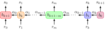
Figure 1: Tensor network representation of the MPO $B^{s_{0},\ldots,s_{k+1}}_{r_{0},\ldots,r_{k}}$.

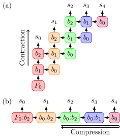
Figure 2: (a) Tensor network representation of $F$ tensor of first five steps with truncation parameter $N_{s}=2$ before contraction. (b) After the contraction, the compression goes through $s_{2}$ to $s_{4}$ only.

The tensor network of $F$ tensor for first five steps is shown graphically in Fig. 2(a) with truncation parameter $N_{s}=2$. Unlike the original QUAPI and TEMPO algorithm, here we do not contract the indices beyond last $N_{s}+1$ steps for which $s_{0}$ and $s_{1}$ are not summed out in the figure. That is, after the iterative propagating process, we shall obtain $F$ as a tensor with indices from $s_{0}$, rather than $s_{N-N_{s}+1}$, to $s_{N}$.

The way we arrange the tensor network shown in Fig. 2(a) is called nonlocal network boundary Jørgensen and Pollock (2019). This nonlocal boundary choice is supposed to be much more inefficient than the local boundary one if there is no truncation $N_{s}$. The reason is that with the nonlocal boundary choice, during each propagating process (35) all time step indices are affected and the MPS compression need to go through all the indices. However, if $N$ is large the calculation would be computationally costly even with the local boundary condition. Therefore we still adopt the nonlocal boundary but with the truncation $N_{s}$, and the compression only goes through the last $N_{s}+1$ steps, as shown in Fig. 2(b).

IV Non-Markovian Effects on $\expectationvalue{\sigma_{z}(t)}$

In this section we study the non-Markovian dynamics of the expectation value $\sigma_{z}(t)$. Starting from an arbitrary initial state (here we starts from $\expectationvalue{\sigma_{z}(0)}=1$), the reduced density matrix would eventually reach a steady state where $\expectationvalue{\sigma_{z}(t)}$ oscillates with frequency $\Omega$. The coherently oscillating $\expectationvalue{\sigma_{z}(t)}$ is just the periodic response signal.

In QUAPI and TEMPO algorithms, the non-Markovianity are controlled by the truncation $N_{s}$. If $N_{s}$ is large enough to cover the non-locality of $\alpha(t)$ (or $\eta_{jk}$) then it is supposed to capture all non-Markovian effects. On the other hand, if $N_{s}=1$ then the dynamics is only relevant to one last time step and thus it gives the Markovian result. In this article, we shall call the $N_{s}=1$ case Markovian, as in Ref. Jørgensen and Pollock (2019).

A set of parameters which induces large amplitude oscillation can be found in Refs. Makarov and Makri (1995a, b). If we set $\Delta=1$, then in our model they correspond to $\Omega=1$, $E=\frac{1}{2}$, $\omega_{c}=3.75$, $T=0.139$ and $\lambda=0.08$. From now on, we shall fix our parameters listed here except the coupling strength $\lambda$. The autocorrelation function $\alpha(t)$ with these parameters are shown in Fig. 3. At $t=\pm 4$, the autocorrelation function already becomes very small.

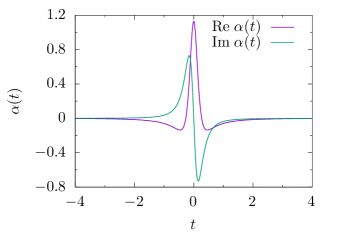
Figure 3: The autocorrelation function $\alpha(t)$ with $\lambda=0.08$, $T=0.139$ and $\omega_{c}=3.75$.

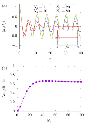
Figure 4: (a) Some typical results of $\expectationvalue{\sigma_{z}(t)}$ with respect to different $N_{s}$. The inset shows a longer time scale for $N_{s}=1$, i.e., Markovian case. (b) The amplitudes of steady coherent oscillation with respect to different $N_{s}$. Here $\lambda=0.08$.

Now we want to cover the non-locality of $\alpha(t)$ shown in Fig. 3, i.e., $N_{s}\delta t\geq 4$. Typical simulations of QUAPI are restricted to $N_{s}<20$ Nalbach et al. (2011); Thorwart et al. (2005), and in fact when $N_{s}$ is greater than 10 it already become time consuming. Therefore the time interval $\delta t$ is usually not less than $0.25$. By employing TEMPO algorithm we go to $N_{s}=80$ in this article, and then $\delta t$ can reach a fairly small value $0.05$.

Some typical results of $\expectationvalue{\sigma_{z}(t)}$ with different $N_{s}$ are shown in Fig. 4(a). It can be seen that the behavior of Markovian $\expectationvalue{\sigma_{z}(t)}$ is qualitatively different from the non-Markovian ones. When $N_{s}=1$ (the Markovian case), $\expectationvalue{\sigma_{z}(t)}$ shows coherent decaying oscillation which decays to a very small (almost zero) oscillation eventually (see the inset of the figure). For non-Markovian cases, even with a not so large $N_{s}=10$, $\expectationvalue{\sigma_{z}(t)}$ reaches steady states fast and then oscillates coherently. When $N_{s}$ increases, the larger amplitude coherent oscillation is induced as the more non-Markovian effects are included. The amplitudes of coherent oscillation with respect to different $N_{s}$ are shown in Fig. 4(b). It can be seen that the amplitude increases as $N_{s}$ increases and becomes stable when $N_{s}\geq 80$. This value corresponds $N_{s}\delta t\approx 4$, at this value most non-Markovian effects are captured.

Figure 5 shows the amplitudes of steady-state oscillation with respect to coupling strength $\lambda$ with different $N_{s}$. For non-Markovian case $N_{s}=80$, a pronounced maximum is demonstrated. This is the sign of QSR phenomenon where the response of a non-linear system to the external periodic driving is enhanced by noise. Note that the maximum of amplitudes is at $\lambda\approx 0.06$ rather than $\lambda=0.08$.

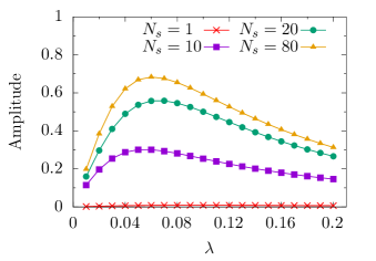
Figure 5: Amplitudes of steady-state oscillation with respect to coupling strength $\lambda$ with different $N_{s}$.

V Non-Markovian Effects on Correlation Function

In this section we study the non-Markovian effects on symmetrized correlation function $C(t_{0},t_{0}+t)$. As mentioned in Sec. II, it is enough to calculate the $t\geq 0$ case.

The correlation function should be evaluated at steady state where $\expectationvalue{\sigma_{z}(t)}$ is doing coherent oscillation, i.e., the time $t_{0}$ should be large enough. It can be seen from Fig. 2(a) that for $\lambda=0.08$, the steady states are reached before $t=40$. Therefore in this case $t_{0}$ should be greater than $40$ when evaluating asymptotic $C(t_{0},t_{0}+t)$. The correlation functions $C(t_{0},t_{0}+t)$ with different $N_{s}$ and some typical $t_{0}$ are shown in Fig. 6. Here we set $t_{0}\geq 200$ which is much larger than 40 to ensure that the correlation function is evaluated in steady state.

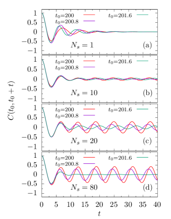
Figure 6: Some typical symmetrized correlation function $C(t_{0},t_{0}+t)$ with different $N_{s}$ and $t_{0}$. Here $\lambda=0.08$.

In Markovian ($N_{s}=1$) case, the reduced dynamics only involves one last time step. Therefore the correlation function obtained in this case just corresponds the quantum regression theorem results Carmichael (1999); Gardiner and Zoller (2004); Breuer (2007). It can be seen from Fig. 6 that the quantum regression theorem misses important non-Markovian effects and gives invalid results, as already mentioned in Refs. Alonso and de Vega (2005); Jørgensen and Pollock (2019). In Markovian case [Fig. 6(a)], correlation function $C(t_{0},t_{0}+t)$ tends to almost zero no matter what value of $t_{0}$. With increasing non-Markovianity, i.e., increasing $N_{s}$, asymptotic $C(t_{0},t_{0}+t)$ does coherent oscillation with increasing amplitude. This is not surprising since such phenomenon is similar to asymptotic $\expectationvalue{\sigma_{z}(t)}$ shown in Fig. 4.

The behavior of $C(t_{0},t_{0}+t)$ depends on $t_{0}$, this can be seen clearly from Fig. 6(d), where the non-Markovian results are shown. Rather than always oscillating with large amplitude, the amplitude varies with different $t_{0}$. When $t_{0}=201.6$, the amplitude can even become very small. This shows that the correlation function $C(t_{0},t_{0}+t)$ contains much more information than mere observable $\expectationvalue{\sigma_{z}(t)}$, and the property of correlation function can not be simply deduced from the behavior of observable.

It can be also seen that with different $t_{0}$, the coherent oscillations have phase difference. This means that the value of $t_{0}$ not only affects the oscillation amplitude but also the oscillation phase. Due to this phase shift, $t_{0}=201.6$ does not cause a minimum oscillation amplitude for $N_{s}=20$ case. In this case, a $t_{0}=201.3$ does it (not shown in the figure).

VI Signal-to-Noise Ratio

A typical way to quantify the response to the driving is the signal-to-noise ratio (SNR) McNamara and Wiesenfeld (1989); Debnath et al. (1989); Löfstedt and Coppersmith (1994); Gammaitoni et al. (1998). QSR occurs when SNR passes through a maximum as the noise level increases. The first papers on SR in fact focused on the behavior of the signal output $\expectationvalue{\sigma_{z}(t)}$, but later the focus shifted to the SNR both theoretically and experimentally.

The time-averaged asymptotic symmetrized correlation function $\bar{C}(t)$ coherently oscillates with the driving frequency $\Omega$ when $t$ is large, therefore the power spectrum $\bar{S}(\omega)$ contains a noise background and $\delta$-function peaks at $\Omega$ and its harmonics. The ratio of the coefficient of the fundamental peak and the value of noise at $\Omega$ is the SNR.

If only considering the fundamental peak, the time-averaged power spectrum can be described as the superposition of a background noise power $N(\omega)$ and a $\delta$ signal term for which

$$\bar{S}(\omega)=G\delta(\omega-\Omega)+N(\omega),$$ (41)

where $G$ is the strength of the signal. The ratio $G/N(\Omega)$ gives the SNR. For sufficiently small driving, $N(\omega)$ does not deviate much from the power spectrum of the undriven system, while for large driving the effect of the signal on the noise need to be taken into consideration.

The correlation function $C(t_{0},t_{0}+t)$ can be split into two parts for which

$$C(t_{0},t_{0}+t)=C_{0}(t_{0},t_{0}+t)+C_{1}(t_{0},t_{0}+t),$$ (42)

where $C_{0}$ is the transient part and $C_{1}$ is the asymptotically coherent oscillation part. Accordingly the time-averaged asymptotic correlation function (8) can be also split into two parts as

$$\bar{C}(t)=\bar{C}_{0}(t)+\bar{C}_{1}(t).$$ (43)

The Fourier transform of coherent oscillation part $\bar{C}_{1}(t)$ just yields delta peak at $\Omega$ and its harmonics, from which the strength of signal $G$ is obtained. Here we simply set $G$ as the amplitude of coherent oscillation $\bar{C}_{1}(t)$, and background noise power $N(\omega)$ is the Fourier transform of $\bar{C}_{0}(t)$. Let $N_{0}(\omega)$ be the background noise power without periodic driving. The background noise powers $N_{0}(\omega)$ and $N(\omega)$ with different $N_{s}$ are shown in Fig. 7.

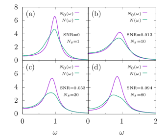
Figure 7: The background noise power with driving $N(\omega)$ and without driving $N_{0}(\omega)$ for different $N_{s}$. Here $\lambda=0.08$.

It should be noted that the shape of $N(\omega)$ presented here is different to those with Gaussian white noise McNamara and Wiesenfeld (1989); Gammaitoni et al. (1998); Joshi (2008) where $N(\omega)$ is roughly a Lorentzian centered at $\omega=0$. Our simulations are in deep quantum regime, the shape of $N(\omega)$ is roughly an asymmetrical “Lorentzian” centered at nonzero $\omega$. In this sense, we are dealing with the color noise.

From Fig. 7, it is clear that the driving force alter the background noise power. In Markovian ($N_{s}=1$) case, the positions of peak of $N_{0}(\omega)$ and $N(\omega)$ are almost the same. But when $N_{s}$ increases, the position of peak of $N(\omega)$ starts deviate from that of $N_{0}(\omega)$. This is most clear in fully non-Markovian case, as shown in Fig. 7(d).

SNR with respect to $\lambda$ for different $N_{s}$ are shown in Fig. 8. It can be seen that, unlike amplitude of $\expectationvalue{\sigma_{z}(t)}$ shown in Fig. 5, for weak noise level $\lambda=0.01$, SNR is almost zero no matter what value of $N_{s}$ is. Besides, SNR reaches its maximum when $\lambda$ is around 0.08, which is different from the position of maximum amplitude of $\expectationvalue{\sigma_{z}(t)}$. This is mostly because the peak position of background noise power $N(\omega)$ is shifted by non-Markovian effects.

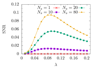
Figure 8: The signal-to-noise ratio with respect to $\lambda$ for different $N_{s}$.

VII Conclusions

In this article, we employ TEMPO algorithm to investigate non-Markovian effects in QSR. For periodic response signal, the signal strength is represented by the amplitude of coherent oscillation of asymptotic $\expectationvalue{\sigma_{z}(t)}$. The QSR is demonstrated by signal strength as a maximum is presented with increasing noise level. The non-Markovianity is controlled by the truncation parameter $N_{s}$. In Markovian limit ($N_{s}=1$), the signal strength is close to zero, which means the response signal almost vanishes. The signal reappears when non-Markovianity is included and its strength becomes larger with more non-Markovianity. This shows the crucial importance of the non-Markovian effects in QSR.

The correlation function $C(t_{0},t_{0}+t)$ contains much more information than mere observable $\expectationvalue{\sigma_{z}(t)}$. Unlike $\expectationvalue{\sigma_{z}(t)}$, whose amplitude simply increases when $N_{s}$ increases, the amplitude of asymptotic $C(t_{0},t_{0}+t)$ also depends on the value of $t_{0}$ in a nontrivial manner. With specific $t_{0}$, the amplitude of asymptotic $C(t_{0},t_{0}+t)$ can be close to zero even for non-Markovian ($N_{s}=80$) case.

The time-averaged correlation function $\bar{C}(t)$ is obtained by averaging correlation function $C(t_{0},t_{0}+t)$ with respect to $t_{0}$ over a period. This $\bar{C}(t)$ can be split into a transient part $\bar{C}_{0}(t)$ and a coherent oscillation part $\bar{C}_{1}(t)$. The Fourier transform of $\bar{C}_{0}(t)$ gives the background noise power $N(\omega)$, and the amplitude of $\bar{C}_{1}(t)$ gives the signal strength. The $N(\omega)$ obtained in our model differs from that from white noise approximation, which indicates that effects of environment in deep quantum regime can be viewed as color noise. When comparing $N(\omega)$ to the background noise power without driving $N_{0}(\omega)$, it is found that their peaks are at almost the same position in Markovian limit. When non-Markovianity is included, the position of their peaks deviate from each other, and this is most clearly seen in fully non-Markovian case. This makes the maximum of SNR and $\expectationvalue{\sigma_{z}(t)}$ appear at different noise level.

Acknowledgments. This work is supported by the NSFC Grant No. 12104328.

References

- Benzi et al. (1981) R. Benzi, A. Sutera, and A. Vulpiani, Journal of Physics A: Mathematical and General 14, L453 (1981).
- Fauve and Heslot (1983) S. Fauve and F. Heslot, Physics Letters A 97, 5 (1983).
- McNamara et al. (1988) B. McNamara, K. Wiesenfeld, and R. Roy, Physical Review Letters 60, 2626 (1988).
- Löfstedt and Coppersmith (1994) R. Löfstedt and S. N. Coppersmith, Physical Review Letters 72, 1947 (1994).
- Gammaitoni et al. (1999) L. Gammaitoni, M. Löcher, A. Bulsara, P. Hänggi, J. Neff, K. Wiesenfeld, W. Ditto, and M. E. Inchiosa, Physical Review Letters 82, 4574 (1999).
- Wagner et al. (2019) T. Wagner, P. Talkner, J. C. Bayer, E. P. Rugeramigabo, P. Hänggi, and R. J. Haug, Nature Physics 15, 330 (2019).
- Hussein et al. (2020) R. Hussein, S. Kohler, J. C. Bayer, T. Wagner, and R. J. Haug, Physical Review Letters 125, 206801 (2020).
- Hänze et al. (2021) M. Hänze, G. McMurtrie, S. Baumann, L. Malavolti, S. N. Coppersmith, and S. Loth, Science Advances 7, eabg2616 (2021).
- McNamara and Wiesenfeld (1989) B. McNamara and K. Wiesenfeld, Physical Review A 39, 4854 (1989).
- Jung (1993) P. Jung, Physics Reports 234, 175 (1993).
- Grifoni and Hänggi (1998) M. Grifoni and P. Hänggi, Physics Reports 304, 229 (1998).
- Gammaitoni et al. (1998) L. Gammaitoni, P. Hänggi, P. Jung, and F. Marchesoni, Reviews of Modern Physics 70, 223 (1998).
- Grifoni et al. (1996) M. Grifoni, L. Hartmann, S. Berchtold, and P. Hänggi, Physical Review E 53, 5890 (1996).
- Grifoni and Hänggi (1996) M. Grifoni and P. Hänggi, Physical Review Letters 76, 1611 (1996).
- Makarov and Makri (1995a) D. E. Makarov and N. Makri, Physical Review B 52, R2257 (1995a).
- Makarov and Makri (1995b) D. E. Makarov and N. Makri, Physical Review E 52, 5863 (1995b).
- Joshi (2008) A. Joshi, Physical Review E 77, 020104 (2008).
- Strathearn et al. (2018) A. Strathearn, P. Kirton, D. Kilda, J. Keeling, and B. W. Lovett, Nature Communications 9, 3322 (2018).
- Schollwöck (2011) U. Schollwöck, Annals of Physics 326, 96 (2011).
- Orús (2014) R. Orús, Annals of Physics 349, 117 (2014).
- Jørgensen and Pollock (2019) M. R. Jørgensen and F. A. Pollock, Physical Review Letters 123, 240602 (2019).
- Fux et al. (2021) G. E. Fux, E. P. Butler, P. R. Eastham, B. W. Lovett, and J. Keeling, Physical Review Letters 126, 200401 (2021).
- Caldeira and Leggett (1983a) A. O. Caldeira and A. J. Leggett, Physica A 121, 587 (1983a).
- Caldeira and Leggett (1983b) A. Caldeira and A. Leggett, Annals of Physics 149, 374 (1983b).
- Leggett et al. (1987) A. J. Leggett, S. Chakravarty, A. T. Dorsey, M. P. A. Fisher, A. Garg, and W. Zwerger, Reviews of Modern Physics 59, 1 (1987).
- Weiss (1993) U. Weiss, Quantum Dissipative Systems (World Scientific, Singapore, 1993).
- Feynman and Vernon (1963) R. P. Feynman and F. L. Vernon, Annals of Physics 24, 118 (1963).
- Feynman and Hibbs (1965) R. P. Feynman and A. R. Hibbs, Quantum Mechanics and Path Integrals (Mc Graw-Hill, New York, 1965).
- Dattani et al. (2012) N. S. Dattani, F. A. Pollock, and D. M. Wilkins, Quantum Physics Letters 1, 35 (2012).
- Makarov and Makri (1993) D. E. Makarov and N. Makri, Physical Review A 48, 3626 (1993).
- Makarov and Makri (1994) D. E. Makarov and N. Makri, Chemical Physics Letters 221, 482 (1994).
- Makri (1995) N. Makri, Journal of Mathematical Physics 36, 2430 (1995).
- Oshiyama et al. (2020) H. Oshiyama, N. Shibata, and S. Suzuki, Journal of the Physical Society of Japan 89, 104002 (2020).
- Oshiyama et al. (2022) H. Oshiyama, S. Suzuki, and N. Shibata, Physical Review Letters 128, 170502 (2022).
- Nalbach et al. (2011) P. Nalbach, A. Ishizaki, G. R. Fleming, and M. Thorwart, New Journal of Physics 13, 063040 (2011).
- Thorwart et al. (2005) M. Thorwart, J. Eckel, and E. R. Mucciolo, Physical Review B 72, 235320 (2005).
- Carmichael (1999) H. J. Carmichael, Statistical Methods in Quantum Optics 1: Master Equations and Fokker-Planck Equations (Springer-Verlag Berlin, Berlin, 1999).
- Gardiner and Zoller (2004) C. W. Gardiner and P. Zoller, Quantum Noise: A Handbook of Markovian and Non-Markovian Quantum Stochastic Methods with Applications to Quantum Optics (Springer-Verlag, Berlin, 2004).
- Breuer (2007) H.-P. Breuer, The Theory of Open Quantum Systems (Oxford University Press, USA, 2007).
- Alonso and de Vega (2005) D. Alonso and I. de Vega, Physical Review Letters 94, 200403 (2005).
- Debnath et al. (1989) G. Debnath, T. Zhou, and F. Moss, Physical Review A 39, 4323 (1989).