On the Practical Power of Automata in Pattern Matching

Abstract

The classical pattern matching paradigm is that of seeking occurrences of one string - the pattern, in another - the text, where both strings are drawn from an alphabet set $\Sigma$. Assuming the text length is $n$ and the pattern length is $m$, this problem can naively be solved in time $O(nm)$. In Knuth, Morris and Pratt’s seminal paper of 1977, an automaton, was developed that allows solving this problem in time $O(n)$ for any alphabet.

This automaton, which we will refer to as the KMP-automaton, has proven useful in solving many other problems. A notable example is the parameterized pattern matching model. In this model, a consistent renaming of symbols from $\Sigma$ is allowed in a match. The parameterized matching paradigm has proven useful in problems in software engineering, computer vision, and other applications.

It has long been suspected that for texts where the symbols are uniformly random, the naive algorithm will perform as well as the KMP algorithm. In this paper we examine the practical efficiency of the KMP algorithm vs. the naive algorithm on a randomly generated text. We analyse the time under various parameters, such as alphabet size, pattern length, and the distribution of pattern occurrences in the text. We do this for both the original exact matching problem and parameterized matching. While the folklore wisdom is vindicated by these findings for the exact matching case, surprisingly, the KMP algorithm works significantly faster than the naive in the parameterized matching case.

We check this hypothesis for DNA texts, and observe a similar behaviour as in the random text. We also show a very structured case where the automaton is much more efficient.

1 Introduction

One of the most well-known data structures in Computer science is the Knuth-Morris-Pratt automaton, or the KMP automaton [20]. It allows solving the exact string matching problem in linear time. The exact string matching problem has input text $T$ of length $n$ and pattern $P$ of length $m$, where the strings are composed of symbols from a given alphabet $\Sigma$. The output is all text locations where the pattern occurrs in the text. The naive way of solving the exact string matching problem takes time $O(nm)$. This can be achieved by sliding the pattern to start at every text location, and comparing each of its elements to the corresponding text symbol. Using the KMP automaton, this problem can be solved in time $O(n)$. In fact, analysis of the algorithm shows that at most $2n$ comparisons need to be done.

It has long been known in the folklore  that if the text is composed of uniformly random alphabet symbols, the naive algorithm’s time is also linear. This belief is bolstered by the fact that the naive algorithm’s mean number of comparisons for text and pattern over a binary alphabet is bounded by

$$n\sum_{i=1}^{m}{i\over 2^{i}}\ {\rm which\ is\ bounded\ by}\ 2n\ {\rm comparisons}.$$

The number of comparisons in the KMP algorithm is also bounded by $2n$. However, because control in the naive algorithm is much simpler, then it may be practically faster than the KMP algorithm.

The last few decades have prompted the evolution of pattern matching from a combinatorial solution of the exact string matching problem  [16, 20] to an area concerned with approximate matching of various relationships motivated by computational molecular biology, computer vision, and complex searches in digitized and distributed multimedia libraries  [15, 7]. An important type of non-exact matching is the parameterized matching problem which was introduced by Baker [10, 11]. Her main motivation lay in software maintenance, where program fragments are to be considered “identical” even if variable names are different. Therefore, strings under this model are comprised of symbols from two disjoint sets $\Sigma$ and $\Pi$ containing fixed symbols and parameter symbols respectively. In this paradigm, one seeks parameterized occurrences, i.e., exact occurrences up to renaming of the parameter symbols of the pattern string in the respective text location. This renaming is a bijection $b:\Pi\rightarrow\Pi$. An optimal algorithm for exact parameterized matching appeared in [5]. It makes use of the KMP automaton for a linear-time solution over fixed finite alphabet $\Sigma$. Approximate parameterized matching was investigated in [10, 17, 8]. Idury and Schäffer [18] considered multiple matching of parameterized patterns.

Parameterized matching has proven useful in other contexts as well. An interesting problem is searching for color images (e.g. [24, 9, 3]). Assume, for example, that we are seeking a given icon in any possible color map. If the colors were fixed, then this is exact two-dimensional pattern matching [2]. However, if the color map is different the exact matching algorithm would not find the pattern. Parameterized two dimensional search is precisely what is needed. If, in addition, one is also willing to lose resolution, then a two dimensional function matching search should be used, where the renaming function is not necessarily a bijection [1, 6].

Parameterized matching can also be naively done in time $O(nm)$. Based on our intuition for exact matching, it is expected that here, too, the naive algorithm is competitive with the KMP automaton-based algorithm of [5] in a randomly generated text.

In this paper we investigate the practical efficiency of the automaton-based algorithm vs. the naive algorithm both in exact and parameterized matching. We consider the following parameters: pattern length, alphabet size, and distribution of pattern occurrences in the text. Our findings are that, indeed, the naive algorithm is faster than the automaton algorithm in practically all settings of the exact matching problem. However, it was interesting to see that the automaton algorithm is always more effective than the naive algorithm for parameterized matching over randomly generated texts. We analyse the reason for this difference.

We established that the randomness of the text is what made the naive algorithm so efficient for exact matching. We, therefore, ran the comparison in a very structured artificial text, and the automaton algorithm was a clear winner.

Having understood the practical behavior of the naive vs. automaton algorithm over randomly generated texts, we were curious if there were “real” texts with a similar phenomenom. We ran the same experiments over DNA texts and observed a similar behavior as that of a randomly generated text.

2 Problem Definition

We begin with basic definitions and notation generally following [13].

Let $S=s_{1}s_{2}\ldots s_{n}$ be a string of length $|S|=n$ over an ordered alphabet $\Sigma$. By $\varepsilon$ we denote an empty string. For two positions $i$ and $j$ on $S$, we denote by $S[i..j]=s_{i}..s_{j}$ the factor (sometimes called substring) of $S$ that begins at position $i$ and ends at position $j$ (it equals $\varepsilon$ if $j<i$). A prefix of $S$ is a factor that begins at position $1$ ($S[1..j]$) and a suffix is a factor that ends at position $n$ ($S[i..n]$).

The exact string matching problem is defined as follows:

Definition 1

(Exact String Matching) Let $\Sigma$ be an alphabet set, $T=t_{1}\cdots t_{n}$ the text and $P=p_{1}\cdots p_{m}$ the pattern, $t_{i},p_{j}\in\Sigma,\ \ i=1,\ldots{},n;j=1,\ldots{},m$. The exact string matching problem is:
input: text $T$ and pattern $P$.
output: All indices $j,\ \ j\in\{1,...,n-m+1\}$ such that

$$t_{j+i-1}=p_{i},\ \ {\rm for\ }i=1,...,m$$

We simplify Baker’s definition of parameterized pattern matching.

Definition 2

(Parameterized-Matching) Let $\Sigma$, $T$ and $P$ be as in Definition 1. We say that $P$ parameterize-matches or simply $p$-matches $T$ in location $j$ if $p_{i}\cong t_{j+i-1},\quad i=1,\ldots{},m$, where $p_{i}\cong t_{j}$ if and only if the following condition holds:
  for every $k=1,\ldots{},i-1,\quad p_{i}=p_{i-k}$ if and only if $t_{j}=t_{j-k}$.

The $p$-matching problem is to determine all $p$-matches of $P$ in $T$.

It two strings $S_{1}$ and $S_{2}$ have the same length $m$ then they are said to parametrize-match or simply $p$-match if $s_{1_{i}}\cong s_{2_{i}}$ for all $i\in\{1,...,m\}$.

Intuitively, the matching relation $\cong$ captures the notion of one-to-one mapping between the alphabet symbols. Specifically, the condition in the definition of $\cong$ ensures that there exists a bijection between the symbols from $\Sigma$ in the pattern and those in the overlapping text, when they $p$-match. The relation $\cong$ has been defined by [5] in a manner suitable for computing the bijection.

Example: The string $ABABCCBA$ parameterize matches the string $XYXYZZYX$. The reason is that if we consider the bijection $\beta:\{A,B,C\}\rightarrow\{X,Y,Z\}$ defined by $A\xrightarrow{\beta}X,\ \ B\xrightarrow{\beta}Y,\ \ C\xrightarrow{\beta}Z$, then we get $\beta(ABABCCBA)=XYXYZZYX$. This explains the requirement in Def. 2, where two sumbols match iff they also match in all their previous occurrences.

Of course, the alphabet bijection need not be as extreme as bijection $\beta$ above. String $ABABCCBA$ also parameterize matches $BABACCAB$, because of bijection $\gamma:\{A,B,C\}\rightarrow\{A,B,C\}$ defined as: $A\xrightarrow{\gamma}B,\ \ B\xrightarrow{\gamma}A,\ \ C\xrightarrow{\gamma}C$.

For completeness, we define the KMP automaton.

Definition 3

Let $P=p_{1}\ldots p_{m}$ be a string over alphabet $\Sigma$. The KMP automaton of $P$ is a 5-tuple $(Q,\Sigma,\delta_{s},\delta_{f},q_{0},q_{a})$, where $Q=\{0,...,m\}$ is the set of states, $\Sigma$ is the alphabet, $\delta_{s}:Q\rightarrow Q$ is the success function, $\delta_{f}:Q\rightarrow Q$ is the failure function, $q_{0}=0$ is the start state and $q_{a}=m$ is the accepting state.

The success function is defined as follows:
$\delta_{s}(i)=i+1$, $i=0,...,m-1$ and
$\delta_{s}(0)=0$

The failure function is defined as follows:
Denote by $\ell(S)$ the length of the longest proper prefix of string $S$ (i.e. excluding the entire string $S$) which is also a suffix of $S$.
$\delta_{f}(i)=\ell(P[1..i]),\ \ {\rm for\ }i=1,..m$.

For an example of the KMP automaton see Fig. 1.

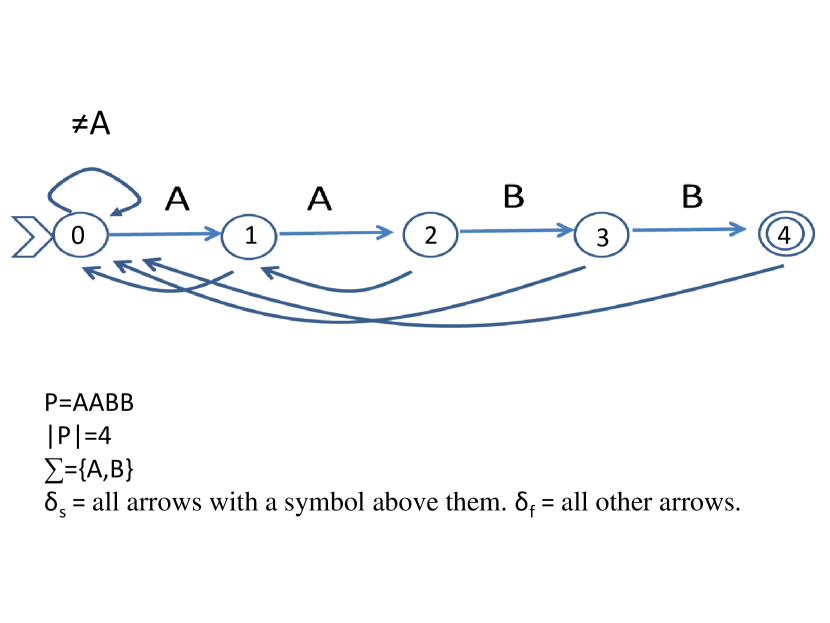
Figure 1: Automaton example

Theorem 1

[20] The KMP automaton can be constructed in time $O(m)$.

3 The Exact String Matching Problem

The Knuth-Morris-Pratt (KMP) search algorithm uses the KMP automaton in the following manner:

Variables:
$pointer_{t}$ points to indices in the text. $pointer_{p}$ points to indices in the pattern.

Initialization:
set pointer $pointer_{t}$ to $1$. set pointer $pointer_{p}$ to $0$.

Main Loop:
While $pointer_{t}\leq n-m+1$ do:
  If $t_{pointer_{t}}=\delta_{s}(pointer_{p})$ then do:
    $pointer_{t}\leftarrow pointer_{t}+1$
    $pointer_{p}\leftarrow\delta_{f}(pointer_{p})$
    If $pointer_{p}=m-1$ then do:
      output “pattern occurrence ends in text location $pointer_{t}$”.
      $pointer_{p}\leftarrow\delta_{f}(m)$
    enddo
  enddo

  else ($t_{pointer_{t}}\neq\delta_{s}(pointer_{p})$) do:
    if $pointer_{p}=0$ then $pointer_{t}\leftarrow pointer_{t}+1$
    else $pointer_{p}\leftarrow\delta_{f}(pointer_{p})$
  enddo
  go to beginning of while loop
endwhile

Theorem 2

[20] The time for the KMP search algorithm is $O(n)$. In fact, it does not exceed $2n$ comparisons.

4 The Parameterized Matching Problem

Amir, Farach, and Muthukrishnan [5] achieved an optimal time algorithm for parameterized string matching by a modification of the KMP algorithm. In fact, the algorithm is exactly the KMP algorithm, however, every equality comparison “$x=y$” is replaced by “$x\cong y$” as defined below.

Implementation of “$x\cong y$”

Construct table $A[1],\ldots{},A[m]$ where $A[i]=$ the largest $k,\quad 1\leq k<i$, such that $p_{k}=p_{i}$. If no such $k$ exists then $A[i]=i$.

The following subroutines compute “$p_{i}\cong t_{j}$” for $j\geq i$, and “$p_{i}\cong p_{j}$” for $j\leq i$.

Compare($p_{i}$,$t_{j}$)
  if $A[i]=i$ and $t_{j}\neq t_{j-1},\ldots{},t_{j-i+1}$ then return equal
  if $A[i]\neq i$ and $t_{j}=t_{j-i+A[i]}$ then return equal
  return not equal
end

Compare($p_{i}$,$p_{j}$)
  if ($A[i]=i$ or $i-A[i]\geq j$) and $p_{j}\neq p_{1},\ldots{},p_{j-1}$ then return equal
  if $i-A[i]<j$ and $p_{j}=p_{j-i+A[i]}$ then return equal
  return not equal
end

Theorem 3

[5] The $p$-matching problem can be solved in $O(n\log\sigma)$ time, where $\sigma={\rm min}(m,|\Sigma|)$.

Proof:

The table $A$ can be constructed in $O(m\log\sigma)$ time as follows: scan the pattern left to right keeping track of the distinct symbols from $\Sigma$ in the pattern in a balanced tree, along with the last occurrence of each such symbol in the portion of the pattern scanned thus far. When the symbol at location $i$ is scanned, look up this symbol in the tree for the immediately preceding occurrence; that gives $A[i]$.

Compare can clearly be implemented in time $O(\log\sigma)$. For the case $A[i]\neq i$, the comparison can be done in time $O(1)$. When scanning the text from left to right, keep the last $m$ symbols in a balanced tree. The check $t_{j}\neq t_{j-1},\ldots{},t_{j-i+1}$ in Compare($p_{i}$,$t_{j}$) can be performed in $O(\log\sigma)$ time using this information. Similarly, Compare($p_{i}$,$p_{j}$) can be performed using $A[i]$. Therefore, the automaton construction in KMP algorithm with every equality comparison “$x=y$” replaced by “$x\cong y$” takes time $O(m\log\sigma)$ and the text scanning takes time $O(n\log\sigma)$, giving a total of $O(n\log\sigma)$ time.

As for the algorithm’s correctness, Amir, Farach and Muthukrishnan showed that the failure link in automaton node $i$ produces the largest prefix of $p_{1}\cdots p_{i}$ that $p$-matches the suffix of $p_{1}\cdots p_{i}$.  

5 Our Experiments

Our implementation was written in $C++$. The platform was Dell latitude 7490 with intel core i7 - 8650U, 32 GB RAM, with 8 MB cache. The running time was computed using the chrono high resolution clock. The random strings were generated using the random Python package.

We implemented the naive algorithm for exact string matching and for parameterized matching. The same code was used for both, except for the implementation of the equivalence relation for parameterized matching, as described above. This required implementing the $A$ array. We also implemented the KMP algorithm for exact string matching, and used the same algorithm for parameterized matching. The only difference was the implementation of the equivalence parameterized matching relation.

The text length $n$ was 1,000,000 symbols. Theoretically, since both the automaton and naive algorithm are sequential and only consider a window of the pattern length, it would have been sufficient to run the experiment on a text of size twice the pattern [4]. However, for the sake of measurement resolution we opted for a large text. Yet the size of 1,000,000 comfortably fits in the cache, and thus we avoid the caching issue. In general, any searching algorithm for patterns of length less than 4MB would fit in the cache if appropriately constructed in the manner of [4]. Therefore our decision gives as accurate a solution as possible.

We ran patterns of lengths $m=32,64,128,256,512,$ and $1024$. The alphabet sizes tested were $|\Sigma|=2,4,6,8,10,20,40,80,160,320$. For each size, 10 tests were run, for a total of 600 tests.

Methodology: We generated a uniformly random text of length $1,000,000$. If the pattern would also be randomly generated, then it would be unlikely to appear in the text. However, when seeking a pattern in the text, one assumes that the pattern occurs in the text. An example would be searching for a sequence in the DNA. When seeking a sequence, one expects to find it but just does not know where. Additionally, we considered the common case where one does not expect many occurrences of the pattern in the text. Consequently, we planted $100$ occurrences of the pattern in the text at uniformly random locations. The final text length was always $1,000,000$. The reason for inserting 100 pattern occurrences is the following. We do not expect manny occurrences, and a 100 occurrences in a million-length text means that less than $0.1\%$ of the text has pattern occurrences. On the other hand, it is sufficient to introduce the option of actually following all elements of the pattern 100 times. This would make a difference in both algorithms. They would both work faster if there were no occurrences at all.

We also implemented a variation where half of the pattern occurrences were in the last quarter of the text. For each alphabet size and pattern length we generated 10 tests and considered the average result of all 10 tests. It should be noted that from a theoretical point of view, the location of the pattern should not make a difference. We tested the different options in order to verify that this is, indeed, the case.

5.1 Exact Matching

5.1.1 Results

Tables 1 and  2 in the Appendix show the alphabet size, the pattern length, the average of the running times of the naive algorithm for the 10 tests, the average of the running time of the KMP algorithm for the 10 tests, and the ratio of the naive algorithm running time over the KMP algorithm running time. Any ratio value below $1$ means that the naive algorithm is faster. A small value indicates a better performance of the naive algorithm. Any value above $1$ indicates that the KMP algorithm is faster than the naive algorithm. The larger the number, the better the performance.

To enable a clearer understanding of the results, we present them below in graph form. The following graphs show the results of our tests for the different pattern lengths. In Figs. 2 and  3, the $x$-axis is the pattern size. The $y$-axis is the ratio of the naive algorithm running time to the KMP algorithm running time. The different colors depict alphabet sizes. In Fig. 2, the patterns were inserted at random, whereas in Fig. 4 the patterns appear at the last half of the text.

To better see the effect of the pattern distribution in the text, Fig. 4 maps, on the same graph, both cases. In this graph, the $x$-axis is the average running time of all pattern lengths per alphabet size, and the $y$-axis is the ratio of the naive algorithm running time to the KMP algorithm running time. The results of the uniformly random distribution are mapped in one color, and the results of all pattern occurrences in the last half of the text are mapped in another.

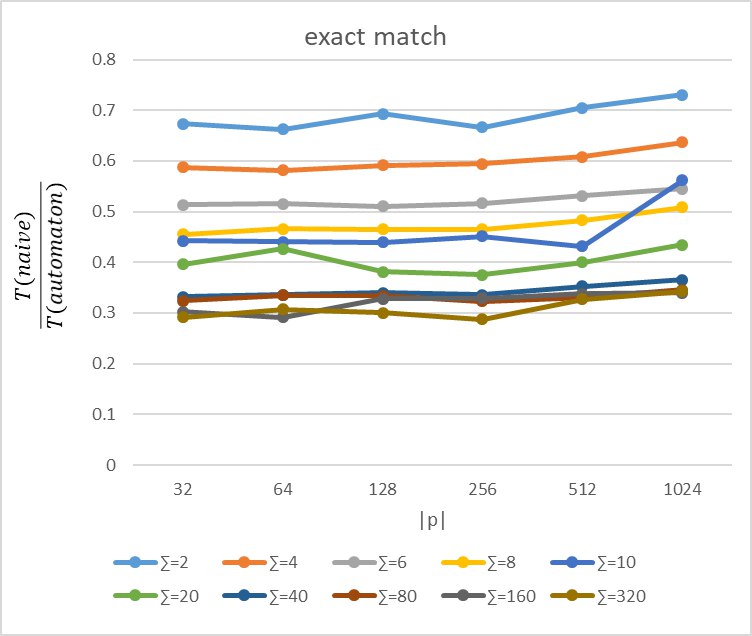
Figure 2: Performance in the Exact Matching case, pattern occurrences distributed uniformly random.

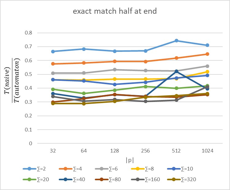
Figure 3: Performance in the Exact Matching case, pattern occurrences congregated at end of text.

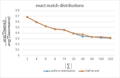
Figure 4: Comparison of average performance of uniform pattern distribution vs. pattern occurrences congregated at end of text.

We note the following phenomena:

1. The naive algorithm performs better than the automaton algorithm. Of the $600$ tests we ran, there were only $3$ instances where the KMP algorithm performed better than the naive, and all were subsumed by the average. In the vast majority of cases the naive algorithm was superior by far.

2. The naive algorithm performs relatively better for larger alphabets.

3. For a fixed alphabet size, there is a slight increase in the naive$/$KMP ratio, as the pattern length increases.

4. The distribution of the pattern occurrences in the text does not seem to make a change in performance.

An analysis of these implementation behaviors appears in the next subsection.

5.1.2 Analysis

We analyse all four results noted above.

Better Performance of the Naive Algorithm
We have seen that the mean number of comparisons of the naive algorithm for binary alphabets is bounded by

$$n\sum_{i=1}^{m}{i\over 2^{i}}\ {\rm which\ is\ bounded\ by}\ 2n\ {\rm comparisons}.$$

The running time of the KMP algorithm is also bounded by $O(2n)$. However, the control of the KMP algorithm is more complex than that of the naive algorithm, which would indicate a constant ratio in favor of the naive algorithm. However, when the KMP algorithm encounters a mismatch it follows the failure link, which avoids the need to re-check a larger substring. Thus, for longer length patterns, where there are more possibilities of following the failure links for longer distances, there is a lessening advantage of the naive algorithm.

Better Performance of the Naive Algorithm for Larger Alphabets
This is fairly clear when we realize that the mean performance of the naive algorithm for alphabet of size $k$ is:

$$n\sum_{i=1}^{m}{i\over k^{i}}\ =n{k\over(k-1)^{2}}\ {\rm comparisons}.$$

This is clearly decreasing the larger the alphabet size. However, the repetitive traversal of the failure link, even in cases where there is no equality in the comparison check, will still raise the relative running time of the KMP algorithm. Here too, the longer the pattern length, the more failure link traversals of the KMP, and thus less overall comparisons, which slightly decreases the advantage of the naive algorithm.

The Distribution of Pattern Occurrences in the Text
If the pattern is not periodic, and if the patterns are not too frequent in the text, then there will be at most one pattern in a text substring of length $2m$. In these circumstances, there is really no effect to the distribution of the pattern in the text. We would expect a difference if the pattern is long with a small period. Indeed, an extreme such case is tested in Subsection 5.1.3.

5.1.3 A Very Structured Example

All previous analyses point to the conviction that the more times a prefix of the pattern appears in the text, and the more periodic the pattern, the better will be the performance of the KMP algorithm. The most extreme case would be of text $A^{n}$ ($A$ concatenated $n$ times), and pattern $A^{m-1}B$. Indeed the results of this case appear in Fig. 5.

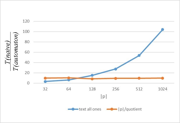
Figure 5: Performance in the Exact Matching case, periodic text.

Theoretical analysis of the naive algorithm predicts that we will have $nm$ comparisons, where $n$ is the text length and $m$ is the pattern length. The KMP algorithm will have $2n$ comparisons, for any pattern length. Thus the ratio $q$ of naive to KMP will be $O({m\over 2})$. In fact, when we plot ${m\over q}$ we get twice the cost of the control of the KMP algorithm. This can be seen in Fig. 5 to be $5$.

5.2 Parameterized Matching

5.2.1 Results

The exact matching results behaved roughly in the manner we expected. The surprise came in the parameterized matching case. Below are the results of our tests. As in the exact matching case, the tables show the alphabet size, the pattern length, the average of the running times of the naive algorithm for the 10 tests, the average of the running time of the automaton-based algorithm for the 10 tests, and the ratio $q$ of the naive algorithm running time over the automaton-based algorithm running time. Any ratio value above $1$ means that the automaton-based algorithm is faster. A large value indicates a better performance of the automaton-based algorithm.

The following graphs show the results of our tests for the different pattern lengths. The $x$-axis is the pattern size. The $y$-axis is the ratio of the naive algorithm running time to the automaton-based algorithm running time. The different colors depict alphabet sizes. To better see the effect of the pattern distribution in the text, we also map, on the same graph, both cases. In this graph, the $x$-axis is the average running time of all pattern lengths per alphabet size, and the $y$-axis is the ratio of the naive algorithm running time to the automaton-based algorithm running time. The results of the uniformly random distribution are mapped in one color, and the results of all pattern occurrences in the last half of the text are mapped in another.

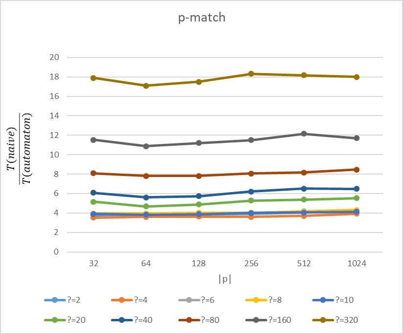
Figure 6: Performance in the Parameterized Matching case, pattern occurrences distributed uniformly random.

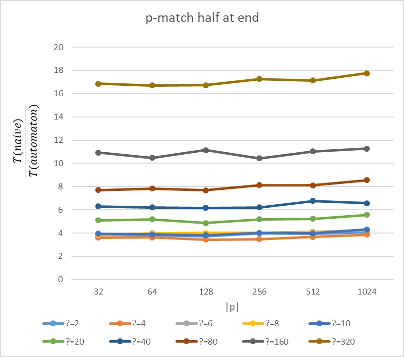
Figure 7: Performance in the Parameterized Matching case, pattern occurrences congregated at end of text.

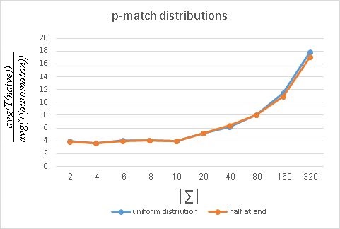
Figure 8: Comparison of average performance of uniform pattern distribution vs. pattern occurrences congregated at end of text.

The parameterized matching results appear in tables 3 and  4 in the appendix. Figs. 6 and 7 map the results of the parameterized matching comparisons for the case where the patterns were inserted at random vs. the case where the patterns appear at the last half of the text. In Fig. 8 we map at the same graph the average results of both the cases where the patterns appear at the text uniformly at random, and where the patterns appear at the last half of the text.

The results are very different from the exact matching case. We note the following phenomena:

1. The automaton-based algorithm always performs significantly better than the naive algorithm.

2. The automaton-based algorithm performs relatively better for larger alphabets.

3. For a fixed alphabet size, the pattern length does not seem to make much difference.

4. The distribution of the pattern occurrences in the text does not seem to make a change in performance.

An analysis of these implementation behaviors and an explanation of the seemingly opposite results from the exact matching case appear in the next subsection.

5.2.2 Analysis

We analyse all four results noted above.

Better Performance of the Automaton-based Algorithm
We have established that the mean number of comparisons for the naive algorithm in size $k$ alphabet is

$$n\sum_{i=1}^{m}{i\over k^{i}}\ =n{k\over(k-1)^{2}}\ {\rm comparisons}.$$

However, when it comes to parameterized matching, any order of the alphabet symbols is a match, thus the mean number of comparisons is to be multiplied by $k!$. Therefore, for size $2$ alphabet we get $4n$ comparisons, and the number rises exponentially with the alphabet size. Also, the automaton-based algorithms is constant at $2n$ comparisons. Even for a size $2$ alphabet, there is twice the number of comparisons in the naive algorithm than in the automaton-based algorithm. Note, also, that because of the need to find the last parameterized match, the control mechanism even of the naive algorithm, is more complex. This results in a superior performance of the automaton-based algorithm even for small alphabets. Of course, the larger the alphabet, the better the performance of the automaton-based algorithm.

Pattern Length

The pattern length does not play a role in the automaton-based algorithm, where the number of comparisons is always bounded by $2n$. In the naive case, the multiplication of the factorial of the alphabet size is so overwhelming that it dominates the pattern length. For example, note that for an extremely large alphabet, there would be a leading prefix of different alphabet symbols. That prefix will always be traversed by the naive algorithm. The larger the alphabet, the longer will be the mean length of that prefix.

Pattern Distribution

As in the exact matching case, for a non-periodic pattern that does not appear too many times, the distribution of occurrences will have no effect on the complexity.

6 DNA Data

Having understood the behavior of the naive algorithm and the automaton-based algorithm in randomly generated texts, the natural question is are there any “real” texts for which the naive algorithm performs better than the automaton-based algorithm.

We performed the same experiments on DNA data. The experimental setting was identical to that of the randomly generated texts with the following differences:

1. The DNA of the fruit fly, Drosophila melanogaster is 143.7 MB long. We extracted 60 subsequences of length 1,000,000 each, as FASTA data from the NIH National Library of Medicine, National Center for Biotechnology Information. We ran 10 tests on each of the six pattern lengths 32, 64, 128, 256, 512, 1024.

2. The alphabet size is 4, due to the four bases in DNA sequence.

Figs. 9 and  10 below show the ratio between the average running time of the naive algorithm and the automaton based algorithm. As in the uniformly random text we see that for the exact matching case the ratio is less than $1$, i.e., the naive algorithm is faster, whereas in the parameterized matching case, the ratio is more than 1, indicating that the automaton based algorithm is faster.

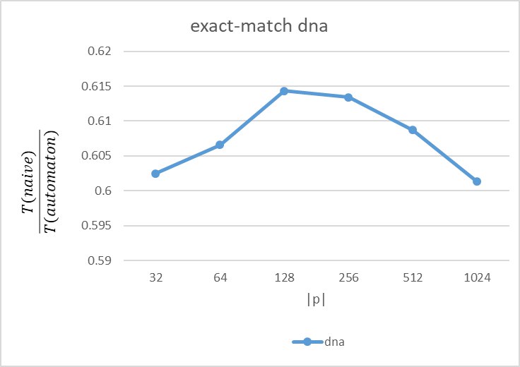
Figure 9: Performance in the Exact Matching case on DNA sequences.

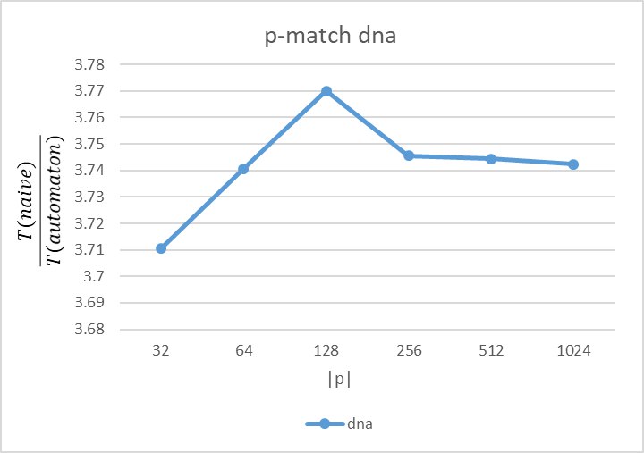
Figure 10: Performance in the Parameterized Matching case on DNA Sequences.

7 Conclusions

The folk wisdom has always been that the naive string matching algorithm will outperform the automaton-based algorithm for uniformly random texts. Indeed this turns out to be the case for exact matching. This study shows that this is not the case for parameterized matching, where the automaton-based algorithm always outperforms the naive algorithm. This advantage is clear and is impressively better the larger the alphabets. The same result is true for searches over DNA data.

The conclusion to take away from this study is that one should not automatically assume that the naive string matching algorithm is better. The matching relation should be analysed. There are various matchings for which an automaton-based algorithm exists. We considered here parameterized matching, but other matchings, such as ordered matching [12, 14, 19], or Cartesian tree matching [21, 22, 23], can also be solved by automaton-based methods. In a practical application it is worthwhile spending some time considering the type of matching one is using. It may turn out to be that the automaton-based algorithm will perform significantly better than the naive, even for uniformly random texts. Alternately, even non-uniformly random data may be such that the naive algorithm performs better than the automaton based algorithm for exact matching.

An open problem is to compare the search time in DNA data to the search time in uniformly random data. While it is clear that DNA data is not uniformly random, it would be interesting to devise an experimental setting to compare search efficiency in both types of strings.

8 Appendix

$|\Sigma|$	patt. length	Naive	KMP	${Naive\over KMP}$	$|\Sigma|$	patt. length	Naive	KMP	${Naive\over KMP}$
2	32	4514.1	6712.5	0.6729	4	32	3174.2	5409.9	0.5879
	64	4449.3	6727.8	0.6623		64	3167.8	5428.3	0.5818
	128	4697.3	6764.3	0.693		128	3136.8	5293.0	0.5917
	256	4522.9	6814.2	0.6666		256	3109.7	5228.2	0.5942
	512	4764.7	6734.7	0.7051		512	3108.8	5110.5	0.608
	1024	4521.4	6188.7	0.7304		1024	3141.1	4928.7	0.6368
6	32	2225.1	4331.2	0.5139	8	32	1771.8	3903.4	0.4553
	64	2199.2	4263.2	0.5157		64	1794.5	3852.4	0.4659
	128	2180.9	4270.6	0.5108		128	1764.0	3789.7	0.4654
	256	2169.2	4201.4	0.5163		256	1766.5	3798.4	0.4652
	512	2193.2	4128.4	0.5314		512	1771.9	3670.6	0.4827
	1024	2238.7	4110.1	0.5455		1024	1827.3	3596.6	0.5085
10	32	1593.1	3598.9	0.4427	20	32	1312.0	3309.2	0.396
	64	1578.3	3586.4	0.44		64	1428.6	3297.7	0.4269
	128	1564.8	3563.9	0.4391		128	1252.7	3264.9	0.3817
	256	1594.5	3531.6	0.4516		256	1187.4	3161.3	0.375
	512	1554.3	3626.0	0.4317		512	1281.7	3166.8	0.4
	1024	1892.5	3380.0	0.5619		1024	1274.6	2923.1	0.4347
40	32	943.9	2846.7	0.3316	80	32	898.1	2758.7	0.3242
	64	964.3	2869.3	0.3358		64	938.4	2777.9	0.335
	128	972.5	2852.5	0.3401		128	946.7	2824.5	0.3336
	256	952.6	2835.3	0.3363		256	875.9	2709.0	0.323
	512	975.4	2769.0	0.3523		512	875.8	2653.9	0.3302
	1024	970.5	2655.4	0.3655		1024	899.6	2605.0	0.346
160	32	810.9	2686.1	0.302	320	32	790.3	2712.0	0.2916
	64	794.0	2733.1	0.2918		64	833.4	2711.1	0.3074
	128	922.2	2771.1	0.3281		128	803.3	2676.3	0.3005
	256	899.2	2700.6	0.3285		256	785.2	2743.0	0.2877
	512	897.8	2635.6	0.3374		512	878.5	2690.4	0.3269
	1024	861.6	2534.9	0.3399		1024	883.8	2563.6	0.3427

Table 1: Implementation Results - Exact Matching, patterns uniformly distributed.

$|\Sigma|$	patt. length	Naive	KMP	${Naive\over KMP}$	$|\Sigma|$	patt. length	Naive	KMP	${Naive\over KMP}$
2	32	4613.3	6931.1	0.6649	4	32	3091.7	5362.9	0.5759
	64	4570.1	6695.7	0.6824		64	3203.2	5499.5	0.5819
	128	4462.8	6702.2	0.667		128	3190.4	5373.6	0.5933
	256	4441.5	6644.9	0.6692		256	3200.3	5413.1	0.5924
	512	4786.4	6441.1	0.744		512	3305.2	5340.0	0.6176
	1024	4493.8	6360.6	0.7105		1024	3322.4	5125.8	0.6469
6	32	2374.7	4638.6	0.509	8	32	1836.3	3978.1	0.4616
	64	2336.6	4586.8	0.5093		64	1804.2	3930.2	0.4589
	128	2467.1	4597.0	0.534		128	1816.9	3908.6	0.465
	256	2350.4	4453.1	0.5274		256	1802.8	3875.2	0.4655
	512	2306.2	4447.2	0.5243		512	1792.0	3832.8	0.4684
	1024	2411.2	4302.9	0.5597		1024	1889.1	3640.7	0.5183
10	32	1741.8	3762.0	0.4608	20	32	1242.4	3173.7	0.3916
	64	1719.8	3772.8	0.4528		64	1173.5	3251.9	0.3615
	128	1616.5	3800.2	0.4264		128	1286.4	3302.4	0.3847
	256	1685.1	3814.7	0.4424		256	1334.3	3234.5	0.411
	512	1774.0	3724.7	0.4737		512	1231.7	3090.4	0.399
	1024	1727.8	3484.3	0.4922		1024	1263.8	3031.5	0.4168
40	32	1108.6	3048.3	0.3606	80	32	867.4	2912.6	0.2988
	64	1014.5	3084.3	0.3283		64	941.2	2912.8	0.3248
	128	1142.9	3210.4	0.3533		128	1023.5	2872.7	0.3546
	256	1026.3	3005.2	0.3413		256	1005.4	2949.3	0.3397
	512	1503.7	2930.9	0.5205		512	956.0	2852.1	0.3355
	1024	1170.1	2926.9	0.3951		1024	954.3	2701.8	0.3532
160	32	981.8	2855.0	0.3393	320	32	769.6	2662.8	0.2894
	64	863.6	2818.4	0.3061		64	771.8	2681.5	0.2882
	128	908.6	2842.8	0.3178		128	799.5	2627.0	0.304
	256	851.2	2796.4	0.3047		256	917.9	2722.0	0.3345
	512	909.6	2917.1	0.313		512	967.3	2757.1	0.3455
	1024	1174.9	2815.9	0.4093		1024	951.2	2601.3	0.3604

Table 2: Implementation Results - Exact Matching, patterns at end.

$|\Sigma|$	patt. length	Naive	KMP	${Naive\over KMP}$	$|\Sigma|$	patt. length	Naive	KMP	${Naive\over KMP}$
2	32	25738.0	6871.8	3.7655	4	32	26104.6	7489.6	3.5351
	64	25996.5	6761.4	3.8593		64	26734.4	7538.6	3.5998
	128	26080.5	6780.8	3.8571		128	26281.4	7370.8	3.6136
	256	26269.7	6688.6	3.934		256	26204.3	7361.0	3.6062
	512	26004.0	6440.3	4.0456		512	26169.6	7123.6	3.71
	1024	26456.0	6277.9	4.2167		1024	26570.9	6863.1	3.924
6	32	26213.2	6818.3	3.96	8	32	26863.5	7229.3	3.9411
	64	26244.3	7022.8	3.8621		64	27010.3	7258.5	3.9394
	128	26130.3	6879.7	3.9429		128	26965.3	7067.4	4.0336
	256	26141.2	6778.1	3.987		256	26918.8	7099.7	4.0304
	512	26212.3	6460.7	4.1752		512	27211.8	6888.9	4.1592
	1024	26171.5	6312.7	4.2986		1024	27406.5	6698.6	4.3042
10	32	28663.6	7629.8	3.8967	20	32	28539.6	5832.4	5.1463
	64	28787.8	7787.6	3.8351		64	28543.3	6329.9	4.6772
	128	28629.8	7664.8	3.8775		128	28254.3	6041.4	4.8694
	256	28647.0	7478.5	3.99		256	28526.7	5733.2	5.2725
	512	28843.4	7406.5	4.0576		512	28326.8	5546.4	5.3728
	1024	28516.9	7074.3	4.1282		1024	28457.7	5433.1	5.5292
40	32	33994.8	5708.6	6.0731	80	32	42524.1	5292.8	8.0792
	64	33826.0	6076.9	5.6046		64	41425.9	5340.1	7.8236
	128	33971.3	5994.7	5.7342		128	41547.1	5387.7	7.8057
	256	33740.9	5544.9	6.2016		256	41489.1	5269.7	8.0644
	512	34501.6	5411.8	6.5045		512	41615.2	5189.5	8.165
	1024	34172.0	5353.9	6.496		1024	42184.8	5067.8	8.478
160	32	54881.0	4789.375	11.5167	320	32	70360.0	3919.7	17.9046
	64	56750.0	5222.7	10.8806		64	75533.8	4456.5	17.1093
	128	57775.6	5212.2	11.2048		128	75098.4	4284.8	17.4987
	256	56719.3	4953.4	11.5		256	77763.7	4238.4	18.328
	512	58276.6	4793.2	12.1498		512	75922.3	4181.3	18.1751
	1024	57331.2	4913.2	11.7029		1024	76831.3	4366.4	17.989

Table 3: Implementation Results - Parameterized Matching, patterns uniformly distributed.

$|\Sigma|$	patt. length	Naive	KMP	${Naive\over KMP}$	$|\Sigma|$	patt. length	Naive	KMP	${Naive\over KMP}$
2	32	26063.4	6801.4	3.8439	4	32	26616.5	7505.3	3.61
	64	26285.3	6878.0	3.828		64	26571.7	7443.4	3.6226
	128	26053.8	7047.4	3.7047		128	26385.6	7829.9	3.4449
	256	26612.5	6671.7	3.996		256	26236.1	7649.5	3.4807
	512	26501.7	6764.8	3.9329		512	26660.5	7356.9	3.6748
	1024	26397.8	6506.4	4.0685		1024	26667.6	7038.6	3.8591
6	32	26312.4	7071.4	3.828	8	32	27246.5	7421.6	3.8491
	64	26733.2	6924.6	3.9976		64	27046.1	7185.0	3.9748
	128	26470.1	7067.1	3.8636		128	27117.6	7170.1	4.009
	256	26346.3	6701.1	4.0218		256	27154.8	7089.7	4.04
	512	26610.6	6682.2	4.117		512	26901.8	6998.0	4.0791
	1024	26632.3	6399.8	4.2563		1024	27227.5	6667.8	4.2963
10	32	29612.8	7759.5	3.9578	20	32	29588.6	6153.9	5.0995
	64	28948.9	7748.2	3.8873		64	29393.4	6010.3	5.1754
	128	29305.1	7925.5	3.829		128	29498.7	6312.8	4.8688
	256	29457.3	7619.7	4.0189		256	29659.5	5966.3	5.1945
	512	29650.7	7836.9	3.9754		512	29067.8	5802.3	5.226
	1024	30742.0	7421.5	4.3099		1024	28922.4	5455.1	5.5624
40	32	34179.7	5577.9	6.2968	80	32	41534.5	5441.2	7.6963
	64	34385.3	5723.2	6.2199		64	41907.7	5373.0	7.8299
	128	34951.8	5758.1	6.1685		128	41709.3	5474.4	7.6894
	256	36703.8	6033.8	6.216		256	41900.3	5211.0	8.1372
	512	37417.4	5682.4	6.7656		512	41753.4	5196.7	8.1023
	1024	35190.1	5488.2	6.5708		1024	43312.9	5074.3	8.5567
160	32	52173.125	4773.875	10.9192	320	32	67440.5	3981.8	16.8561
	64	54173.0	5176.9	10.4658		64	71874.8	4294.4	16.7108
	128	56313.9	5032.4	11.1442		128	72359.4	4315.2	16.725
	256	54897.4	5257.0	10.433		256	72268.3	4179.1	17.2654
	512	55123.0	5025.2	11.0268		512	72729.5	4234.7	17.1366
	1024	55603.0	4915.0	11.26		1024	73777.8	4152.8	17.7372

Table 4: Implementation Results - Parameterized Matching, patterns at end.

References

- [1] A. Amir, A. Aumann, M. Lewenstein, and E. Porat. Function matching. SIAM Journal on Computing, 35(5):1007–1022, 2006.
- [2] A. Amir, G. Benson, and M. Farach. An alphabet independent approach to two dimensional pattern matching. SIAM J. Comp., 23(2):313–323, 1994.
- [3] A. Amir, K. W. Church, and E. Dar. Separable attributes: a technique for solving the submatrices character count problem. In Proc. 13th ACM-SIAM Symp. on Discrete Algorithms (SODA), pages 400–401, 2002.
- [4] A. Amir and M. Farach. Efficient 2-dimensional approximate matching of half-rectangular figures. Information and Computation, 118(1):1–11, April 1995.
- [5] A. Amir, M. Farach, and S. Muthukrishnan. Alphabet dependence in parameterized matching. Information Processing Letters, 49:111–115, 1994.
- [6] A. Amir and I. Nor. Generalized function matching. J. of Discrete Algorithms, 5(3):514–523, 2007.
- [7] A. Apostolico and Z. Galil (editors). Pattern Matching Algorithms. Oxford University Press, 1997.
- [8] A. Apostolico, M. Lewenstein, and P. Erdös. Parameterized matching with mismatches. Journal of Discrete Algorithms, 5(1):135–140, 2007.
- [9] G.P. Babu, B.M. Mehtre, and M.S. Kankanhalli. Color indexing for efficient image retrieval. Multimedia Tools and Applications, 1(4):327–348, Nov. 1995.
- [10] B. S. Baker. Parameterized pattern matching: Algorithms and applications. Journal of Computer and System Sciences, 52(1):28–42, 1996.
- [11] B. S. Baker. Parameterized duplication in strings: Algorithms and an application to software maintenance. SIAM Journal on Computing, 26(5):1343–1362, 1997.
- [12] S. Cho, J. C. Na, K. Park, and J. S. Sim. Fast order-preserving pattern matching. In Proc. 7th conf. Combinatorial Optimization and Applications COCOA, volume 8287 of Lecture Notes in Computer Science, pages 295–305. Springer, 2013.
- [13] M. Crochemore, C. Hancart, and T. Lecroq. Algorithms on Strings. Cambridge University Press, 2007.
- [14] M. Crochemore, C.S. Iliopoulos, T. Kociumaka, M. Kubica, A. Langiu, S.P. Pissis, J. Radoszewski, W. Rytter, and T. Walen. Order-preserving incomplete suffix trees and order-preserving indexes. In Proc. 20th International Symposium on String Processing and Information Retrieval (SPIRE), volume 8214 of LNCS, pages 84–95. Springer, 2013.
- [15] M. Crochemore and W. Rytter. Text Algorithms. Oxford University Press, 1994.
- [16] M.J. Fischer and M.S. Paterson. String matching and other products. Complexity of Computation, R.M. Karp (editor), SIAM-AMS Proceedings, 7:113–125, 1974.
- [17] C. Hazay, M. Lewenstein, and D. Sokol. Approximate parameterized matching. In Proc. 12th Annual European Symposium on Algorithms (ESA 2004), pages 414–425, 2004.
- [18] R.M. Idury and A.A Schäffer. Multiple matching of parameterized patterns. In Proc. 5th Combinatorial Pattern Matching (CPM), volume 807 of LNCS, pages 226–239. Springer-Verlag, 1994.
- [19] J. Kim, A. Amir, J.C. Na, K. Park, and J.S. Sim. On representations of ternary order relations in numeric strings. In Proc. 2nd International Conference on Algorithms for Big Data (ICABD), volume 1146 of CEUR Workshop Proceedings, pages 46–52, 2014.
- [20] D.E. Knuth, J.H. Morris, and V.R. Pratt. Fast pattern matching in strings. SIAM J. Comp., 6:323–350, 1977.
- [21] S. G. Park, A. Amir, G. M. Landau, and K. Park. Cartesian Tree Matching and Indexing. In Nadia Pisanti and Solon P. Pissis, editors, Proc. 30th Symposium on Combinatorial Pattern Matching (CPM), volume 128 of Leibniz International Proceedings in Informatics (LIPIcs), pages 16:1–16:14, 2019.
- [22] S. G. Park, M. Bataa, A. Amir, G. M. Landau, and K. Park. Finding patterns and periods in cartesian tree matching. Theor. Comput. Sci., 845:181–197, 2020.
- [23] S. Song, G. Gu, C. Ryu, S. Faro, T. Lecroq, and K. Park. Fast algorithms for single and multiple pattern cartesian tree matching. Theor. Comput. Sci., 849:47–63, 2021.
- [24] M. Swain and D. Ballard. Color indexing. International Journal of Computer Vision, 7(1):11–32, 1991.