Planetary systems with forces other than gravitational forces

Abstract

A discrete and exact algorithm for obtaining planetary systems is derived in a recent article (Eur. Phys. J. Plus 2022, 137:99). Here the algorithm is used to obtain planetary systems with forces different from the Newtonian inverse square gravitational forces. A Newtonian planetary system exhibits regular elliptical orbits, and here it is demonstrated that a planetary system with pure inverse forces also is stable and with regular orbits, whereas a planetary system with inverse cubic forces is unstable and without regular orbits. The regular orbits in a planetary system with inverse forces deviate, however, from the usual elliptical orbits by having revolving orbits with tendency to orbits with three or eight loops. Newton’s Proposition 45 in Principia for the Moon’s revolving orbits caused by an additional attraction to the gravitational attraction is confirmed, but whereas the additional inverse forces stabilize the planetary system, the additional inverse cubic forces can destabilize the planetary system at a sufficient strength.

I Introduction

Our world consists of objects with collections of atoms and molecules which are bound together by ionic or covalent bonds. On a larger length scale these objects are collected in planetary systems in galaxies, which are bound together by gravitational forces. The ionic and covalent bonds are established by electromagnetic forces whereas the planetary systems and the galaxies are hold together by gravitational forces. Although the two forces differ enormously in strength by a factor of $\approx 10^{36}$ they have, however, some common features. The radial strengths of both forces are proportional to the inverse square (ISF), $r^{-2}$, of the distances between mass centers , and both forces are believed to extend to infinity. The two forces can also result in regular closed orbits for the dynamics of a collection of force centres, as is demonstrated by our solar system and the orbitals of the bounded electrons at a atomic nucleus. The two other fundamental forces are the strong and weak nuclear forces and they are both short ranged. All other forces are ”derived forces” such as the harmonic forces or the attractive induced dipole-dipole forces.

Isaac Newton formulated the classical mechanics in his book PHILOSOPHIÆ NATURALIS PRINCIPIA MATHEMATICA ($Principia$) Newton1687 , where he also proposed the law of gravity and solved Kepler’s equation for a planets motion. According to Newton, gravity varies with the inverse square of the distance $r$ between two celestial objects, and a planet exposed to the gravitational force from the Sun moves in an elliptical orbit. The Moon exhibits, however, periodic ”revolving orbits” and Newton shows in $Principia$ that this behaviour, which is caused by the daily rotation of the Earth, could be taken into account by and additional inverse cubic force proportional to $r^{-3}$ (ICF). But it raises the question: for which forces can a system of objects have regular orbits?

It is only possible to solve the classical mechanics differential equations for two objects. The classical second-order differential equation for the dynamics of two objects with a central force proportional to $r^{n}$ can be solved for a series of values of the power $n$ . An important result was obtained by Bertrand Bertrand , who proved that all bound orbits are closed orbits. Later investigations have proved the existence of regular orbits for a series of values of the power $n$ of the central force, including the ICF Whittaker ; Broucke1980 ; Mahomed2000 .

For a system consisting of many objects, the dynamics of coupled harmonic oscillators demonstrates that it indeed is possible to have stable regular dynamics for systems with other forces than the gravitational forces, but else there is no theoretical proofs, nor any other examples of that it is possible. Here it is, however, demonstrated by Molecular Dynamics simulations (MD) of planetary systems Toxvaerd2022 , that a planetary system also can have planets with stable regular orbits for attractive forces which varies as
$-r^{-1}$
$-r^{-2}\pm\alpha\times r^{-1}$
$-r^{-2}\pm\alpha\times r^{-3}$ for $\alpha\in[-100,10]$.
But it has not been possible to obtain stable regular orbits for $r^{-3}$.

II The force between two spherically symmetrical objects

Newton was aware of that the extension of an object can affect the gravitational force between two objects, and in Theorem XXXI in $Principia$ Newtonshell he also solved this problem for ISF between spherically symmetrical objects.

Newton’s Theorem XXXI states that:

1. A spherically symmetrical body affects external objects gravitational as though all of its mass were concentrated at a point at its center.

2. If the body is a spherically symmetric shell no net gravitational force is exerted by the shell on any object inside, regardless of the object’s location within the shell.

Newtons theorem is, however, only valid for ISF. The forces between spherically symmetrical objects with forces proportional to $r^{-1}$, inverse forces (IF), or ICF depends on the objects extension. Newton’s derivation of the theorem is by the use of Euclidean geometry, but the forces between two spherically symmetrical objects can also be derived by the use of algebra.

Let the objects No. $i$ and $j$ be spherically symmetrical with masses $m_{i}$ and $m_{j}$ and with a uniform density within the balls with the radii $\sigma_{i}$ and $\sigma_{j}$. The attraction, IF, ISF or ICF, on a mass $\delta m_{i}$ at $\textbf{s}_{i}$ in object $i$ and at the distance $s_{ij}$ from a mass $\delta m_{j}$ at $\textbf{s}_{j}$ in $j$ is

$$\delta\mathbf{F}_{ij}=-\beta\delta m_{i}\delta m_{j}s_{ij}^{n}\hat{\mathbf{s}}_{ij},$$ (1)

with $n$=-1, -2 and -3, respectively, and the total force $\textbf{F}_{ij}$ is obtained by a quadruple integration, first between $\delta m_{i}$ at $\textbf{s}_{i}$ and mass elements $\delta m_{j}$ in a sphere in $j$ with radius $\sigma_{j}^{{}^{\prime}}\leq\sigma_{j}$, then over spheres centred at $\textbf{r}_{j}$ with radius $\sigma_{j}^{{}^{\prime}}$, and then correspondingly between mass $m_{j}$ located in the center, $\textbf{r}_{j}$ and mass elements $\delta m_{i}$.

Consider mass elements $\delta m_{j}(\textbf{s}_{j})=4\pi\sigma_{j}^{{}^{\prime}2}m_{j}d\sigma^{\prime}_{j}/(4\pi/3\sigma_{j}^{3})$ at $\textbf{s}_{j}$ in a thin shell $[\sigma^{\prime}_{j},\sigma^{\prime}_{j}+d\sigma^{\prime}_{j}]$ with center at $\textbf{r}_{j}$ and a distance $r^{\prime}_{ij}=\mid\textbf{s}_{i}-\textbf{r}_{j}\mid>\sigma_{i}+\sigma_{j}\geq\sigma_{i}+\sigma^{\prime}_{j}$ to $\textbf{s}_{i}$. The force $\delta\textbf{F}_{ij}=-\beta\delta m_{i}m_{j}s_{ij}^{n}\hat{\textbf{r}}^{\prime}_{ij}$ on $\delta m_{i}$ from object $j$ is WikipediaNewtonshell

$$\delta\mathbf{F}_{ij}=-\beta\frac{\delta m_{i}}{4r_{ij}^{{}^{\prime}2}}\int_{0}^{\sigma_{j}}\frac{\delta m_{j}}{\sigma^{\prime}_{j}}\int^{r^{\prime}_{ij}+\sigma^{\prime}_{j}}_{r^{\prime}_{ij}-\sigma^{\prime}_{j}}s_{ij}^{n}[s_{ij}^{2}+r_{ij}^{{}^{\prime}2}-\sigma_{j}^{{}^{\prime}2}]ds_{ij}\hat{\mathbf{r}}^{\prime}_{ij}.$$ (2)

The integrals are very simple for ISF since

$$-\beta\frac{\delta m_{i}}{4r_{ij}^{{}^{\prime}2}}\int_{0}^{\sigma_{j}}\frac{\delta m_{j}}{\sigma^{\prime}_{j}}\int^{r^{\prime}_{ij}+\sigma^{\prime}_{j}}_{r^{\prime}_{ij}-\sigma^{\prime}_{j}}s_{ij}^{-2}[s_{ij}^{2}+r_{ij}^{{}^{\prime}2}-\sigma_{j}^{{}^{\prime}2}]ds_{ij}$$ (3)

$$=-\beta\frac{\delta m_{i}}{4r_{ij}^{{}^{\prime}2}}\int_{0}^{\sigma_{j}}\frac{\delta m_{j}}{\sigma^{\prime}_{j}}4\sigma^{\prime}_{j}=-\beta\frac{\delta m_{i}m_{j}}{r_{ij}^{{}^{\prime}2}},$$

and the integration over shells centred at $\textbf{r}_{i}$ with mass elements $\delta m_{i}$ leads to $Theorem$ $XXXI$.

The integrations are more complex for $n\neq-2$. The simplest way to proceed is to expand the first integral in powers of $\sigma^{\prime}_{j}/r^{\prime}_{ij}$. The first terms in the final expressions for the force between $i$ and $j$ are given below.

For the IF function $s^{-1}$:

$$\mathbf{F}_{ij}(r_{ij})\simeq-\frac{\beta_{1}m_{i}m_{j}}{r_{ij}}(1-\frac{\sigma_{i}^{2}+\sigma_{j}^{2}}{5r_{ij}^{2}})\hat{\mathbf{r}}_{ij}+\mathcal{O}(r_{ij}^{-4})$$ (4)

For $s^{-2}$ one obtains the usual expression for the gravitational ISF force ($\beta_{2}=G$) which does not depend on the extensions of the two spherically symmetrical objects

$$\mathbf{F}_{ij}(r_{ij})=-\frac{Gm_{i}m_{j}}{r_{ij}^{2}}\hat{\mathbf{r}}_{ij}.$$ (5)

For $s^{-3}$ the ICF radial force is

$$\mathbf{F}_{ij}(r_{ij})=-\frac{\beta_{3}m_{i}m_{j}}{r_{ij}^{3}}(1+\frac{2\sigma_{i}^{2}+2\sigma_{j}^{2}}{5r_{ij}^{2}})\hat{\mathbf{r}}_{ij}+\mathcal{O}(r_{ij}^{-6}).$$ (6)

The dynamics of planetary systems with the different kind of gravitational attractions is given in the next Section.

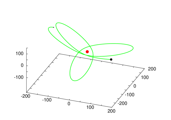
Figure 1: A loop of the innermost planet from a position at time $t=2.5\times 10^{6}$, marked by a big black sphere to a position at $t=2.5007325\times 10^{6}$ (293000 discrete time steps), marked by a small black sphere. The position of the ”Sun” is with an enlarged red sphere. Some simultaneous loops of two other planets in the planetary system are shown in the next figure.

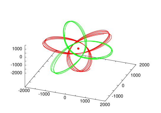
Figure 2: The simultaneous orbits with bows for two other planets in the planetary system. The orbits are obtained for one million discrete time steps in the time interval $t\in[2.5\times 10^{6},2.5025\times 10^{6}]$.

III Dynamics of planetary systems with different gravitational forces

A discrete and exact algorithm for obtaining planetary systems is derived in a recent article Toxvaerd2022 . The algorithm is symplectic and time reversible and has the same invariances as Newton’s analytic dynamics. For Kepler’s solution of the two body system of a Sun and a planet one can compare the two dynamics Toxvaerd2020 , which leads to the same orbits. The discrete dynamics is absolute stable and without any adjustments for conservation of energy, momentum and angular momentum for billion of time steps. The algorithm and how to obtain planetary systems is given in the Appendix. Here the algorithm is used to obtain planetary systems with forces different from the Newtonian inverse square gravitational forces.

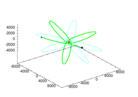
Figure 3: Bows in a loop with green and light blue for the outermost planet. The start position at $t=2.5\times 10^{6}$ is marked with a big black sphere and the first three bows is with green color. The position at $t=2.5025\times 10^{6}$ after the first three bows is shown by a smaller black sphere, and the succeeding five bows is with light blue. Several consecutive loops of the planet are shown in Figure 5.

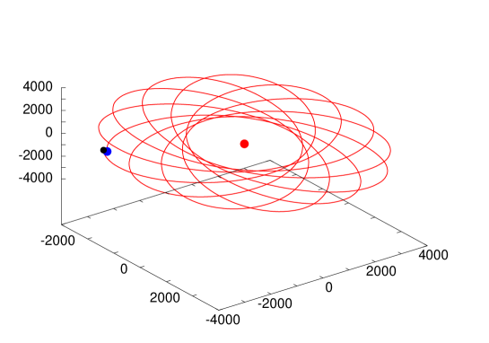
Figure 4: A planet which after 13 orbits almost returns to its start position. The start position at $t=2.5\times 10^{6}$ is shown with a big blue sphere, and the position at $t=2.5051975\times 10^{6}$ after thirteen orbits by a smaller black sphere. The next figure shows several orbits of the planet together with the orbits of the outermost planet.

III.1 Planetary systems for objects with inverse forces

The IF between two objects $i$ and $j$ is given by the Eq. (4). The Eq. (4) gives the first-order size-correction for the forces between spherically symmetrical uniform mass objects. The investigation is conducted in two ways by MD simulations. A: One can simply create planetary systems in the same way as described in Toxvaerd2022 and in the Appendix, or alternatively B: one can replace the Newtonian ISF forces between objects in an ordinary planetary system by the corresponding inverse IF forces.

A: The results of obtaining planetary systems spontaneously by merging of objects as in Toxvaerd2022 are shown in the next Figures. Planetary systems with strength $\beta_{1}=1$ were created spontaneously at time $t=0$ from different configurations, distributions of velocities and masses $m_{i}(0)=1$ of objects. (For units of length, time and strength of the attractions in the MD systems see the Appendix.) Ten different planetary systems were formed and the overall result and conclusion from the ten systems is, that it is easily to obtain planetary systems with IF forces. But the regular orbits deviate, however, qualitatively from the elliptical orbits in an ordinary planetary system. A typical regular orbit is shown in Figure 1.

Figure 1 shows a loop of the innermost planet in one of the ten planetary systems, which was simulated with IF. The planetary system was started with thousand objects and the planetary system with IF contained 38 planets after $10^{9}$ MD time steps corresponding to a MD time $t=2.5\times 10^{6}$, and where the inner planets have performed several thousand bound rotations. The planet in Figure 1 performs a loop, but with a change of its elliptical major axis by $\approx\pi/3$ at the passage of the ”Sun”, by which the total regular orbit appears with three consecutive bows with an angle of $\approx 2\pi/3$. The total angular momentum for the system is conserved by Newton’s exact discrete algorithm Toxvaerd2022 , but also the angular momentum of the individual planets in the system are conserved to a high degree so the three bows are in the same plane. Most of the planets exhibit this regular dynamics. Figure 2 shows the simultaneous orbits for two other planets in the same planetary system. The planetary system with the object shown in Figure 1 and Figure 2 consists of 38 objects in bound orbits around a central heavy object (the ”Sun” with $m_{\textrm{Sun}}$=867). In Broucke1980 Broucke has obtained the orbit for one planet (Figure 2 in Broucke1980 ). There is, however, only some similarities between the present orbits for a many-body three dimensional planetary system and the 2D orbit of a single planet.

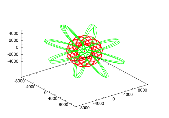
Figure 5: The outermost planet (green) together with the planet from Figure 4 (red) with its orbits in bands. The outermost planet changes its major orbit axis with $\approx\pi/4$ at every past of the Sun. The central Sun is with red.

All the planets in the planetary systems with inverse forces show, what Newton probably would have called revolving orbits, but not all of the planets have orbits of the form shown in Figure 1 and Figure 2. The next figure, Figure 3, show the consecutive bows of the outermost planet in the same planetary system. The planet changes its principal axis by $\approx\pi/4$ by which it performs eight bows in its regular orbit. Figure 5 shows with green 3-4 loops of this planet together with another planet in the same planetary system.

It has not been possible to obtain simple elliptical regular orbits, but there are examples of planets with a smaller change of their principal axis at the passage of the Sun. Figure 4 gives such an example of a planet, which after thirteen loops return to its start position, and a collection of consecutive loops for this planet, shown by red in Figure 5, demonstrates that this regular pattern is maintained over many consecutive loops.

B: Planetary systems with IF forces were obtained in another way by replacing the Newtonian ISF forces in an ordinary planetary system with the IF forces. The discrete dynamics with IF was started with the end-positions of the planet in the planetary system Toxvaerd2022 . A replacement with $\beta_{1}=\beta_{2}=G$ results in a collapse of the planetary systems and with only two planets in revolving orbits similar to the orbits shown in Figure 2. The other planets were engulfed by the Sun. This is due to that the inverse forces with $\beta_{1}=\beta_{2}=G$ and acting on a planet are about a thousand time stronger than the Newtonian gravitational forces. Planets in the Newtonian planetary systems in Toxvaerd2022 are located at mean distances to their Suns at $<r_{i,Sun}>\approx[100,30000]$. For an ordinary planet with a Newtonian ISF force field and at a position $r_{i,Sun}=1000$ the corresponding IF force is of the order thousand time stronger than the Newtonian ISF force. So in order to establish whether it is possible to obtain simple elliptical orbits without revolving orbits, the forces in the Newtonian planetary systems in Toxvaerd2022 were replaced with IF forces and with $\beta_{1}\approx G/1000$. The replacement was performed in the following way:

A planet $i$ with a rather circular orbit and at a mean distance $<r_{i,Sun}>\approx 1000$ was selected and the strength $\beta_{1}=0.00105$ was determined so the planet follow the same elliptical orbit shortly after the replacement. The result of this replacement of the forces in the planetary system on the orbit of this planet is shown in Figure 6, which show the orbit of an ordinary planet before( red) and after (green) the replacement. The replacement is for $\beta=0.00105$ for which the planet followed the gravitational orbit (red) over a long period of time before it deviated and exhibited the revolving orbits shown in the figure, but with a small change of its principal axis by passage at the Sun and with elliptical-like orbits. The other planet in the Newtonian planetary system changed their orbits to the revolving orbits (blue orbit Figure 6), also shown in the previous figures.

It has not been possible to obtain simple elliptical orbits, which spontaneously appears in an ordinary Newtonian planetary system. The simulations were performed by the first order IF expression, Eq. 4, but simulations with- and without the first order correction $\mid\delta\textbf{F}_{\textrm{IF}}\mid=\beta_{1}m_{i}m_{j}(\sigma_{i}^{2}+\sigma_{j}^{2})/5r_{ij}^{3}$ showed, that the first-order correction only has a minor quantitative effect, and that the exclusion of this term do not change the overall qualitative result.

III.2 Simulation of systems with inverse cubic forces

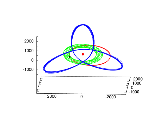
Figure 6: The red elliptical orbits is for a planet with Newtonian ISF forces and the green orbits are after the forces at the position marked with a black sphere is replaced with IF forces and with $\beta_{1}$=0.00105 by which the planet in a short time follow the elliptical path before the revolving behaviour. The orbit (blue) of a planet at a mean distance slightly bigger than the planet shown by red changed spontaneously its elliptical orbit to the bows also shown in the previous figures.

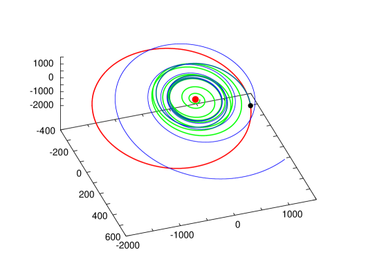
Figure 7: The orbits for a planet in a planetary system with ICF. The planetary system is obtained from an ordinary planetary system and with elliptical orbits (red) by replacing the ISF forces by ICF and with a strength $\beta_{3}\approx 1230\times G$. The black circles is the position of the planet at the time where the replacement took place and the green curve is for $\beta_{3}=1228.75$ and the blue curve is for $\beta_{3}=1228.5$.

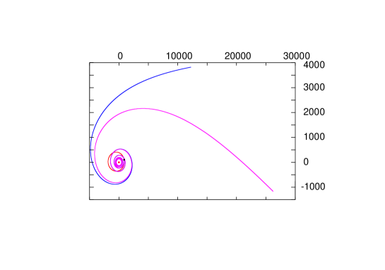
Figure 8: Top view of the orbits of the planet also shown in details in the previous figure. The blue curve is for ICF with Eq. (6) and the magenta curve is with the zero-order ICF $-1228.5m_{i}m_{j}/r_{ij}^{3}$.

A system of objects with masses $m_{i}(0)=1$ and pure ICF given by Eq. (6) does not self-assemble to a planetary system. The objects either fuse together or expand as free objects. This observation is valid for different values of the gravitational constant $\beta_{3}$ in Eq. (6) and it was not possible to create a planetary system with ICF.

Another way to demonstrate the instability of planetary systems with pure ICF attractions is to replace the Newtonian gravitational ISF in a planetary system by ICF as described in the previous subsection. Thus it is possible to determine a values of $\beta_{3}\pm\delta$, by which a given planet in an Newtonian planetary system either engulfs by the Sun by changing the forces from $-G/r^{2}$ to $-(\beta_{3}+\delta)/r^{3}(1+(2\sigma_{i}^{2}+2\sigma_{j}^{2})/5r_{ij}^{2})$ or leaves the Sun as a free object for $\beta_{3}-\delta$. Figure 7 shows this ”tipping point” for the same planetary system and planet as is shown in Figure 6 with red for ISF and green for IF. The planet with pure ICF is engulfed by the Sun for $\beta_{3}+\delta=1228.75$ (green curve), but escapes the Sun for $\beta_{3}-\delta=1228.5$ (blue curve). The Eq. (6) is with the first asymptotic correction in a rapid converging expansion for the extension of the spherically symmetrical objects with an uniform density. The zero order expression for the ICF system: $-\beta_{3}m_{i}m_{j}/r_{ij}^{3}$ gives the same qualitatively result, as shown in Figure 8. The tipping point is the same either one includes the first order correction or not.

IV Newton’s proportions for the Moon’s revolving orbits

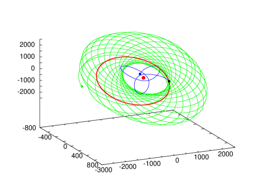
Figure 9: The planet also shown in Figure 7 with red, but now with IF or ICF included in the ISF attraction. The orbit with red is with pure ISF; the orbit with green is with ICF: $\alpha_{3}/r^{3}=-100/r^{3}$ included from the position marked by a black sphere, and the orbit with blue is with the IF: $\alpha_{1}/r=0.01/r$ included. The planet with ISF + ICF (green) has revolved $\approx$ 23-24 times before the principal axis in the elliptical orbit has changed $2\pi$.

The Moon exhibits apsidal precession, which is called Saroscyclus and it has been known since ancient times. Newton shows in Proposition 43-45 in $Principia$, that the added force on a single object from a fixed mass center which can cause its apsidal precession must be a central force between the planet and a mass point fixed in space (the Sun). In Proposition 44 he shows that an inverse-cube force (ICF) might causes the revolving orbits, and in Proposition 45 Newton extended his theorem to arbitrary central forces by assuming that the particle moved in nearly circular orbit Chandrasekhar1995 . The Moon’s apsidal precession is explained by flattering by the rotating Earth with tide waves, which causes an ICF on the Moon. For Newton’s analyse of the Moon’s apsidal precession see Aoki1992 .

New investigations of isotopes from the Moon reveal that it was created $\approx$ 4.51 billion year ago and $\approx$ 50 to 60 million years after the emergence of the Earth and our solar system Barboni2017 ; Thiemens2019 , and the Earth contained the Hadean ocean(s) with tide waves shortly after the creation of the Moon Harrison , so an ICF has not affect the overall stability of the Moon’s regular orbit. The rotation of the Earth and the Moon’s orbit around the Earth results in an ICF which has accelerated the Moon out to its present position with its apsidal precession. The early orbit of the Moon may have had a high eccentricity Zuber2006 , but it is difficult to determine the evolution of the Moon’s orbit due to the many factors which influence its evolution Green2017 . One can, however, conclude that the presence of an additional force on the Moon due to the tide waves has not affected the overall stability of the Moon’s regular orbit.

The planetary system and the orbit shown with red in Figure 7 are simulated with either ICF or IF included in the attractions. The planetary system is affected by including an $\alpha_{3}r^{-3}$ ICF, and the systems are destroyed for $\alpha_{3}\geq 100$. The ISF planetary system with the planet shown in Figure 7 with red contains twenty one planets and only three survived by including $100*r^{-3}$ in the attraction whereas all twenty one planets remained in regular orbits for ICF with $\alpha_{3}\leq 10*r^{-3}$.

The orbits in a planetary system with ISF+ICF forces exhibit the revolving behaviour predicted by Newton: Figure 9 shows the orbit of the planet, also shown in Figure 7, with red without additional attractions, with (green) with ISF+ICF and with $\alpha_{3}=-100$, and with blue with ISF+IF and with $\alpha_{1}=0.01$. The behaviour of ISF+ICF and ISF+IF is in agreement with Newton’s $Proposition$ $45$. Inclusion of IF in the gravitational attractions enhances, however, the revolving behaviour and stabilizes the planetary system, whereas inclusion of the ICF also results in revolving orbits, but it destabilizes the planetary system. The planetary ISF+ICF system is not stable for $\alpha_{3}>100$ and for pure ICF attractions.

V Conclusion

The discrete algorithm (Appendix A), derived in Toxvaerd2022 is used to obtain planetary system with forces other than gravitational forces. The main conclusion is, that it is easy to obtain planetary systems with inverse gravitational forces. However, it is not possible to obtain planetary systems with inverse cubic gravitational forces, even if one smoothly replaces the inverse square gravitational forces in a stable planetary system with inverse cubic forces. A detailed investigation of the planetary system after the replacement of the forces shows, that one can determine a strength of the gravitational constant $\beta_{3}$ for inverse cubic forces for which a planet either detaches itself from the planetary system for $\beta_{3}-\delta$, or are engulfed by the ”Sun” for $\beta_{3}+\delta$ (Figure 7 and Figure 8). So the attractions in our universe with inverse square forces for the gravitational attractions between masses and the Coulomb attractions between charges is the limit value for regular orbits. A system of objects will, for inverse attractions with $\propto r^{-n}$ with $n\geq 3$, have the well known thermodynamic behaviour with gas-liquid-solid phases, but without regular orbits between units in the system.

The orbits of the planets in a planetary systems with pure inverse forces have ”revolving orbits”. The regular orbits deviate, however, significantly from the slightly perturbed elliptic orbits in an ordinary planetary with additional weak non-gravitational attractions. The principal axis changes with $\approx\pi/3$ at every loops (Figure 1, Figure 2, Figure 6 for the main part of the regular orbits in a planetary system with inverse forces. But also changes with $\pi/4$ is observed (Figure 3 and Figure 5) together with other smaller, but rather constant changes (Figure 4 and Figure 5).

Newton stated in Proposition 43-45 in $Principia$, that the Moons revolving orbits could be explained by an additional attraction, $r^{-n}$, to the gravitational attraction with $n\neq 2$. The present simulations of planetary systems with gravitational attractions and an additional attractions with either $n=1$ or $n=3$ confirm Newton’s Propositions, but whereas attractions with additional inverse attractions stabilize the planetary systems, the inclusion of a weak inverse cubic attractions also gives ” revolving orbits” (Figure 9), but it will destabilize the planetary system by adding sufficient strong inverse cubic attractions to the inverse square gravitational forces.

VI Appendix

The gravitational force, $\textbf{F}_{i}(\textbf{r}_{i})$, on a planet $i$ at $\textbf{r}_{i}$ in a planetary systems with $N$ celestial objects is

$$\mathbf{F}_{i}(\textbf{r}_{i})=\sum_{j\neq i}^{N}\mathbf{F}_{ij}(r_{ij})$$ (7)

where the summations over forces $\textbf{F}(r_{ij})$ is given by one of the Eqn 4-6.

Newton derived the discrete central difference algorithm when he obtained his second law Toxvaerd2020 . In Newton’s classical discrete dynamics Newton1687 ; Toxvaerd2020 a new position $\textbf{r}_{k}(t+\delta t)$ at time $t+\delta t$ of an object $k$ with the mass $m_{k}$ is determined by the force $\textbf{f}_{k}(t)$ acting on the object at the discrete positions $\textbf{r}_{k}(t)$ at time $t$, and the position $\textbf{r}_{k}(t-\delta t)$ at $t-\delta t$ as

$$m_{k}\frac{\textbf{r}_{k}(t+\delta t)-\textbf{r}_{k}(t)}{\delta t}=m_{k}\frac{\textbf{r}_{k}(t)-\textbf{r}_{k}(t-\delta t)}{\delta t}+\delta t\textbf{f}_{k}(t),$$ (8)

where the momenta $\textbf{p}_{k}(t+\delta t/2)=m_{k}(\textbf{r}_{k}(t+\delta t)-\textbf{r}_{k}(t))/\delta t$ and $\textbf{p}_{k}(t-\delta t/2)=m_{k}(\textbf{r}_{k}(t)-\textbf{r}_{k}(t-\delta t))/\delta t$ are constant in the time intervals in between the discrete positions. Newton postulated Eq. (A2) and obtained his second law, and the analytic dynamics in the limit $lim_{\delta t\rightarrow 0}$.

The algorithm, Eq. (A2), is usual presented as the ”Leap frog” algorithm for the velocities

$$\textbf{v}_{k}(t+\delta t/2)=\textbf{v}_{k}(t-\delta t/2)+\delta t/m_{k}\textbf{f}_{k}(t).$$ (9)

The positions are determined from the discrete values of the momenta/velocities as

$$\textbf{r}_{k}(t+\delta t)=\textbf{r}_{k}(t)+\delta t\textbf{v}_{k}(t+\delta t/2).$$ (10)

Let all the spherically symmetrical objects have the same (reduced) number density $\rho=(\pi/6)^{-1}$ by which the diameter $\sigma_{i}$ of the spherical object $i$ is

$$\sigma_{i}=m_{i}^{1/3}$$ (11)

and the collision diameter

$$\sigma_{ij}=\frac{\sigma_{i}+\sigma_{j}}{2}.$$ (12)

If the distance $r_{ij}(t)$ at time $t$ between two objects is less than $\sigma_{ij}$ the two objects merge to one spherical symmetrical object with mass

$$m_{\alpha}=m_{i}+m_{j},$$ (13)

and diameter

$$\sigma_{\alpha}=(m_{\alpha})^{1/3},$$ (14)

and with the new object $\alpha$ at the position

$$\textbf{r}_{\alpha}(t)=\frac{m_{i}}{m_{\alpha}}\textbf{r}_{i}(t)+\frac{m_{j}}{m_{\alpha}}\textbf{r}_{j}(t),$$ (15)

at the center of mass of the the two objects before the fusion. (The object $\alpha$ at the center of mass of the two merged objects $i$ and $j$ might occasionally be near another object $k$ by which more objects merge, but after the same laws.)

The momenta of the objects in the discrete dynamics just before the fusion are $\textbf{p}^{N}(t-\delta t/2)$ and the total momentum of the system is conserved at the fusion if

$$\textbf{v}_{\alpha}(t-\delta t/2)=\frac{m_{i}}{m_{\alpha}}\textbf{v}_{i}(t-\delta t/2)+\frac{m_{j}}{m_{\alpha}}\textbf{v}_{j}(t-\delta t/2),$$ (16)

which determines the velocity $\textbf{v}_{\alpha}(t-\delta t/2)$ of the merged object.

The algorithm for planetary system consists of the equations (A3)+(A4) for time steps without merging of objects, and the fusion of objects is given by the equations (A6),(A7), (A8), (A9) and (A10).

Newtons discrete algorithm (A3), which is used in almost all MD simulations, is usually called the Verlet- or Leap-frog algorithm and it has the same invariances as his exact analytic dynamics Toxvaerd2022 ; Toxvaerd1994 ; Toxvaerd2012 . The invariances are maintained by the extension to planetary systems (A6),(A7), (A8), (A9) and (A10) Toxvaerd2022 .

The gravitational strengths in the article are in units of $\beta_{i}^{*}=G=1$ and the mass $m_{i}(0)=1$ and diameters of the planets $\sigma_{i}(0)=1$ at the start time $t=0$. For units and set-up of the systems see also Toxvaerd2022 . The planetary systems in the articles are obtained for thousand objects, which at $t=0$ are separated with a mean distance $<r_{ij}>\approx 1000$ and with a Maxwell-Boltzmann distributed velocities with mean velocity $<v_{i}>\approx 1$, for the set-up of the systems see also Toxvaerd2022 . The systems are followed at least $10^{9}$ MD time steps, i.e. $t=2.5\times 10^{6}$ time-units, which corresponds to $\approx 10^{3}$ to $10^{4}$ orbits for a planet.

References

- (1) Newton, I.: PHILOSOPHIÆ NATURALIS PRINCIPIA MATHEMATICA. LONDINI, Anno MDCLXXXVII. Second Ed.1713; Third Ed. 1726
- (2) Bertrand, J.: The Théoremè relatif au mouvement d’un point attiré vers un centre fixe. C. R. Acad. Sci. 77, 849-853 (1873)
- (3) Whittaker, E. T.: A Treatise on the Analytical Dynamics of Particles and Rigid Bodies, with an Introduction to the Problem of Three Bodies (4th ed.). New York: Dover Publications
- (4) Broucke, R.: Notes on the central force . Astrophys. Space Sci. 72, 33-53 (1980)
- (5) Mahomed, F.M., Vawda, F.: Application of Symmetries to Central Force Problems. Nonlinear Dyn. 21, 307-315 (2000)
- (6) Toxvaerd, S.: An algorithm for coalescence of classical objects and formation of planetary systems. Eur. Phys. J. Plus, 137:99 2022
- (7) Toxvaerd S.: Newton’s disctret dynamics. Eur. J. Phys. 135, 267 (2020)
- (8) , THEOREM XXXI.
- (9) Wikipedia: Newton’s shell theorem.
- (10) , Proportion 43-45
- (11) Chandrasekhar, S.: Newton’s Principia for the common reader, Oxford Univ. Press (1995)
- (12) Aoki, S.: The Moon-Test in Newton’s Principia: Accuracy of Inverse-Square Law of Universal Gravitation. Arch. Hist. Exact Sci. 44, 147 (1992)
- (13) M. Barboni, M., Boehnke, P., Keller, B., Kohl, I., Schoene, B., Young, E.D., McKeegan, K.D.: Early formation of the Moon 4.51 billion years ago. Sci. Adv. 3: e1602365 (2107)
- (14) Thiemens, M.M., Sprung, P., Fonseca, R.O.C., Leitzke, F.P., Münker, C.: Early Moon formation inferred from hafnium-tungsten systematics. Nat. Geosci. 12, 696 (2019)
- (15) Harrison, T.M.: The Hadean Crust: Evidence from ¿4 Ga Zircons. Annu. Rev. Earth Planet Sci. 37, 479 (2009)
- (16) Garrick-Bethell, I., Wisdom, J., Zuber, M.T.: Evidence for a Past High-Eccentricity Lunar Orbit. Science 313, 652 (2006)
- (17) Green, J.A.M., Huber,M., Waltham, D., Buzan, J., Wells, M.: Explicitly modelled deep-time tidal dissipation and its implication for Lunar history. Earth Planet Sci. Lett. 461, 46 (2017)
- (18) Toxvaerd S.: Hamiltonians for discrete dynamics. Phys. Rev. E 50, 2271 (1994)
- (19) Toxvaerd, S., Heilmann, O.J., Dyre, J.C.: Energy conservation in molecular dynamics simulations of classical systems J. Chem. Phys. 136, 224106 (2012)