Exact and asymptotic goodness-of-fit tests based on the maximum and its location of the empirical process

Abstract

The supremum of the standardized empirical process is a promising statistic for testing whether the distribution function $F$ of i.i.d. real random variables is either equal to a given distribution function $F_{0}$ (hypothesis) or $F\geq F_{0}$ (one-sided alternative). Since Jaeschke (1979) it is well-known that an affine-linear transformation of the suprema converge in distribution to the Gumbel law as the sample size tends to infinity. This enables the construction of an asymptotic level-$\alpha$ test. However, the rate of convergence is extremely slow. As a consequence the probability of the type I error is much larger than $\alpha$ even for sample sizes beyond $10.000$. Now, the standardization consists of the weight-function $1/\sqrt{F_{0}(x)(1-F_{0}(x))}$. Substituting the weight-function by a suitable random constant leads to a new test-statistic, for which we can derive the exact distribution (and the limit distribution) under the hypothesis. A comparison via a Monte-Carlo simulation shows that the new test is uniformly better than the Smirnov-test and an appropriately modified test due to Mason and Schuenemeyer (1983). Our methodology also works for the two-sided alternative $F\neq F_{0}$.

1 Introduction

Let $X_{1},\ldots,X_{n}$ be $n\in\mathbb{N}$ independent and identically distributed real random variables defined on a probability space $(\Omega,\mathcal{A},\mathbb{P})$ and with common distribution function $F$. Throughout the paper it is assumed that $F$ is continuous. Given a (continuous) distribution function $F_{0}$ we want to test the hypothesis $H_{0}:F=F_{0}$ versus the alternative $H_{1}:F\neq F_{0},F\geq F_{0}$. If

$$F_{n}(x)=\frac{1}{n}\sum_{i=1}^{n}1_{\{X_{i}\leq x\}},\;x\in\mathbb{R},$$

is the empirical distribution function, then the well-known Smirnov-statistic is given by

$$M_{n}:=\sup_{x\in\mathbb{R}}\{F_{n}(x)-F_{0}(x)\}=\max_{1\leq i\leq n}\{\frac{i}{n}-F_{0}(X_{i:n})\},$$ (1)

where $X_{i:n}$ denotes the $i-$th order statistic and the equality holds almost surely (a.s.). By the Glivenko-Cantelli Theorem $D_{n}:=F_{n}-F_{0}$ converges a.s. to $D=F-F_{0}$ uniformly on $\mathbb{R}$. In order to make the Smirnov-test more sensitive for deviations of $F$ from $F_{0}$ in the tails of $F_{0}$ one could use

$$W_{n}:=\sup_{x:0<F_{0}(x)<1}\frac{F_{n}(x)-F_{0}(x)}{\sqrt{F_{0}(x)(1-F_{0}(x))}}.$$

Here,

$$Q_{n}(x):=\frac{F_{n}(x)-F_{0}(x)}{\sqrt{F_{0}(x)(1-F_{0}(x))}}\rightarrow Q(x)=\frac{F(x)-F_{0}(x)}{\sqrt{F_{0}(x)(1-F_{0}(x))}}$$

a.s. for every $x\in\mathbb{R}$ with $0<F_{0}(x)<1$. The following example shows that this approach seems to be very promising.

Example 1.

Let $\tau\in\mathbb{R}$ and $\delta>1$. Define $F=F_{\tau,\delta}$ by

$$F(x):=\left\{\begin{array}[]{l@{\quad,\quad}l}\delta F_{0}(x)&x\leq\tau\\ \beta(F_{0}(x)-F_{0}(\tau))+\delta F_{0}(\tau)&x>\tau,\end{array}\right.$$

If $\delta F_{0}(\tau)<1$ and $\beta$ satisfies (*) $\delta F_{0}(\tau)+\beta(1-F_{0}(\tau))=1$, then $F$ is a distribution function. Further, one verifies that

$$D(x)=\left\{\begin{array}[]{l@{\quad,\quad}l}(\delta-\beta)(1-F_{0}(\tau))F_{0}(x)&x\leq\tau\\ (\delta-\beta)F_{0}(\tau)(1-F_{0}(x))&x>\tau,\end{array}\right.$$

and thus

$$Q(x)=\left\{\begin{array}[]{l@{\quad,\quad}l}(\delta-\beta)(1-F_{0}(\tau))\sqrt{F_{0}(x)/(1-F_{0}(x))}&x\leq\tau\\ (\delta-\beta)F_{0}(\tau)\sqrt{(1-F_{0}(x))/F_{0}(x)}&x>\tau.\end{array}\right.$$

Since $\delta>1$ and therefore by (*) $\beta<1$ we see that $\delta-\beta$ is positive and hence $D=F-F_{0}>0$. This shows that $F$ lies in the alternative $H_{1}$. Moreover it follows that $\tau$ is a maximizing point of $D$ and $Q$ as well. In particular

$$M:=\max_{x\in\mathbb{R}}D(x) =(\delta-\beta)F_{0}(\tau)(1-F_{0}(\tau))$$

$$<(\delta-\beta)\sqrt{F_{0}(\tau)(1-F_{0}(\tau))}=\sup_{x:0<F_{0}(x)<1}Q(x)=:S.$$

Thus the supremum $S$ is larger than the maximum $M$ by the factor $1/\sqrt{F_{0}(\tau)(1-F_{0}(\tau))}$, which increases to infinity as $F_{0}(\tau)\rightarrow 0$ or $F_{0}(\tau)\rightarrow 1$. Recall that we are interested in detecting deviations in the tails of $F_{0}$. For instance if $F_{0}(\tau)=0.01$ then the supremum $S$ is about ten times larger than the maximum $M$, namely $S=10.0504*M$. Now both tests reject the hypothesis for large values of $M_{n}\approx M$ and $W_{n}\approx S$, whence we strongly expect that the $W_{n}$-test is much more likely to indicate the alternative than the Smirnov-test.

So, as far as the behaviour on the alternative is concerned the $W_{n}$-test should be the better candidate. However, a serious problem occurs when we want to determine the critical values or $p$-values. Here we need the exact or at least asymptotic distribution of the underlying test-statistics $M_{n}$ and $W_{n}$. In case of $M_{n}$ the exact and the asymptotic distribution are known since the publication of Smirnov (1944):

$$\mathbb{P}(M_{n}\leq x)=1-\sum_{i=0}^{[n(1-x)]}x{n\choose i}(x+\frac{i}{n})^{i-1}(1-x-\frac{i}{n})^{n-i},\quad 0<x<1,$$ (2)

where $[\cdot]$ denotes the floor function. From the exact formula Smirnov (1944) deduces the asymptotic distribution as $n\rightarrow\infty$:

$$\mathbb{P}(\sqrt{n}M_{n}\leq x)\rightarrow 1-\exp\{-2x^{2}\},\;x\geq 0.$$

In contrast to $M_{n}$ an explicit expression for the distribution function of $W_{n}$ for finite sample size $n\in\mathbb{N}$ is not known in the literature. Even worse, Chibisov (1966) shows that $W_{n}$ converges to infinity in probability, whence the construction of an asymptotic level-$\alpha$ test fails. But there is a way out by the following limit theorem of Jaeschke (1979):

$$\mathbb{P}(\sqrt{n}W_{n}\leq\frac{x+b_{n}}{a_{n}})\rightarrow e^{-e^{-x}}\;\forall\;x\in\mathbb{R},$$ (3)

where $a_{n}=\sqrt{2\log\log n}$ and $b_{n}=2\log\log n+\frac{1}{2}\log\log\log n-\frac{1}{2}\log\pi$. Thus

$$c_{\alpha,n}=\frac{-\log(-\log(1-\alpha))+b_{n}}{a_{n}}$$

yields that

$$\mathbb{P}(W_{n}>c_{\alpha,n})\rightarrow\alpha$$

and therefore the test with rejection region $\{W_{n}>c_{\alpha,n}\}$ is an asymptotic level-$\alpha$ test. Unfortunately the convergence in (3) to an extreme-value distribution (Gumbel) is known to be very (very) slow. As a consequence there are poor approximations of the exact critical values by $c_{\alpha,n}$ even for large sample sizes $n$. In particular, the probability of the type I error is much larger than the given level $\alpha$ of significance. For instance given $\alpha=0.1$ and $n=30,300,5000,10.000$ the true probabilities of type I error are equal to $0.18913,0.18524,0.18388,0.18211$, which are more than $1.8$ times greater than the required level of significance. If $\alpha=0.01$ the factor increases dramatically. Indeed even for the very large sample size $n=10.000$ the true error probability is equal to $0.0671$ and thus more than six times bigger! From this point of view the $W_{n}$-test is unacceptable and we look for an alternative. (We obtained the above probabilities by a Monte-Carlo simulation with $10^{5}$ replicates upon noticing that $W_{n}$ is distribution-free under the hypothesis $H_{0}$.)

Let us explain the basic idea for the construction of our new test. Assume the alternative $F$ is such that $D=F-F_{0}$ has a unique maximizing point $\tau$ (as for instance when $F$ is as in the above example). To make the test still sensitive for small deviations of $F$ from $F_{0}$ in the tails of $F_{0}$ we replace the weight function $1/\sqrt{F_{0}(x)(1-F_{0}(x))}$ by the constant $1/\sqrt{F_{0}(\tau)(1-F_{0}(\tau)}$. Since $\tau$ is unknown we estimate it by

$$\tau_{n}:=\raisebox{-5.12149pt}{${{\displaystyle\rm arg\,\!max}\atop{\scriptstyle x\in[0,1]}}$}\{F_{n}(x)-F_{0}(x\})\stackrel{{\scriptstyle a.s.}}{{=}}X_{R:n},$$

where

$$R:=\raisebox{-5.12149pt}{${{\displaystyle\rm arg\,\!max}\atop{\scriptstyle 1\leq i\leq n}}$}\frac{i}{n}-F_{0}(X_{i:n}):=\min\{1\leq k\leq n:\frac{i}{n}-F_{0}(X_{i:n})\leq\frac{k}{n}-F_{0}(X_{k:n})\;\forall\;1\leq i\leq n\}.$$

By (1) the estimator $\tau_{n}$ is the smallest maximizing point of $D_{n}=F_{n}-F_{0}$. According to Corollary 2.3 of Ferger (2005) $\tau_{n}$ converges to $\tau$ a.s. (In fact Ferger (2005) considers minimizing points of $D_{n}$, but the arguments there can easily be carried over to maximizing points.) Herewith it follows that

$$Q_{n}^{*}(x):=\frac{F_{n}(x)-F_{0}(x)}{F_{0}(\tau_{n})(1-F_{0}(\tau_{n}))}\rightarrow Q^{*}(x)=\frac{F(x)-F_{0}(x)}{F_{0}(\tau)(1-F_{0}(\tau))}$$

a.s. for each $x\in\mathbb{R}$. Our test rejects the hypothesis $H_{0}$ for large values of

$$W_{n}^{*}:=\sup_{x\in\mathbb{R}}Q_{n}^{*}(x)=\frac{M_{n}}{\sqrt{F_{0}(X_{R:n})(1-F_{0}(X_{R:n}))}}=\frac{\frac{R}{n}-F_{0}(X_{R:n})}{\sqrt{F_{0}(X_{R:n})(1-F_{0}(X_{R:n}))}}.$$

In the situation of the above example one has that

$$Q^{*}(x)=\left\{\begin{array}[]{l@{\quad,\quad}l}(\delta-\beta)\sqrt{(1-F_{0}(\tau))/F_{0}(\tau)}F_{0}(x))&x\leq\tau\\ (\delta-\beta)\sqrt{F_{0}(\tau)/(1-F_{0}(\tau))}(1-F_{0}(x))&x>\tau\end{array}\right.$$

and consequently $\sup_{x\in\mathbb{R}}Q^{*}(x)=\sup_{x\in\mathbb{R}}Q(x)=S$. Thus there is good hope that the $W_{n}^{*}$-test has a power on $H_{1}$ comparably as good as the $W_{n}$-test. But in contrast to the latter we can determine not only the asymptotic but also the finite sample null-distribution of $W_{n}^{*}$.

Our methodology also works in case of the two-sided alternative $H_{2}:F\neq F_{0}$. Here, the Kolmogorov-Smirnov statistic

$$K_{n}=\sup_{x\in\mathbb{R}}|F_{n}(x)-F_{0}(x)|=\max_{1\leq i\leq n}\max\{i/n-F_{0}(X_{i:n}),(i-1)/n-F_{0}(X_{i:n})\}$$ (4)

again can be made more sensitive by weighting with $1/\sqrt{F_{0}(x)(1-F_{0}(x))}$. The resulting statistic

$$V_{n}=\sup_{x:0<F_{0}(x)<1}\frac{|F_{n}(x)-F_{0}(x)|}{\sqrt{F_{0}(x)(1-F_{0}(x))}}$$

exhibits the same problems as its one-sided counterpart $W_{n}$: There is no explicit formula for its finite sample size distribution and $\sqrt{n}V_{n}\stackrel{{\scriptstyle\mathbb{P}}}{{\rightarrow}}\infty$. However by Jaeschke (1979)

$$\mathbb{P}(\sqrt{n}V_{n}\leq\frac{x+b_{n}}{a_{n}})\rightarrow e^{-2e^{-x}}\;\forall\;x\in\mathbb{R},$$ (5)

but again the rate of convergence is extremely slow. As an alternative test-statistic we introduce

$$V_{n}^{*}:=\frac{K_{n}}{\sqrt{F_{0}(\sigma_{n})(1-F_{0}(\sigma_{n}))}},$$

where $\sigma_{n}$ is the (smallest) maximizing point of $|F_{n}-F_{0}|$. Some elementary considerations show that $\sigma_{n}=X_{r:n}$, where

$$r=\raisebox{-5.12149pt}{${{\displaystyle\rm arg\,\!max}\atop{\scriptstyle 1\leq i\leq n}}$}\max\{\frac{i}{n}-F_{0}(X_{i:n}),F_{0}(X_{i:n})-\frac{i-1}{n}\}.$$

In particular, $V_{n}^{*}$ can be computed by the formula

$$V_{n}^{*}=\frac{\max\{\frac{r}{n}-F_{0}(X_{r:n}),F_{0}(X_{r:n})-\frac{r-1}{n}\}}{\sqrt{F_{0}(X_{r:n})(1-F_{0}(X_{r:n}))}}.$$

In contrast to its one-sided counterpart $W_{n}^{*}$ the exact distribution of $V_{n}^{*}$ is not known, but we are still able to derive its limit distribution.

By the quantile-transformation the statistics $M_{n},W_{n},K_{n}$ and $V_{n}$ are distribution-free under the hypothesis. We will see that our statistics $W_{n}^{*}$ and $V_{n}^{*}$ share this property, see Lemma .1.

Notice that $V_{n}$ is a generalized Kolmogorov-Smirnov statistic

$$K_{n,\Phi}=\sup_{0<F_{0}(x)<1}|F_{n}(x)-F_{0}(x)|\Phi(F_{0}(x))$$ (6)

and $W_{n}$ is a generalized Smirnov statistics

$$S_{n,\Phi}=\sup_{0<F_{0}(x)<1}\{F_{n}(x)-F_{0}(x)\}\Phi(F_{0}(x))$$ (7)

pertaining to $\Phi(u)=1/\sqrt{u(1-u)}$. Utilization of generalized statistics as in (6) and (7) with $\Phi:(0,1)\rightarrow[0,\infty)$ is not new in the literature and in fact has a long history. We give a few examples. Renyi (1953) considers $\Phi(u)=1_{[a,1]}(u)u^{-1}$ with fixed $0<a<1$. His motivation was to measure the relative error (on the region $\{F_{0}\geq a\})$ rather than the absolute error. He derives the limit distributions of $\sqrt{n}K_{n,\Phi}$ and $\sqrt{n}S_{n,\Phi}$ under $F=F_{0}$, whereas the exact distribution of $K_{n,\Phi}$ and $S_{n,\phi}$ has been found by Takacs (1967) and Ishii (1959), respectively. Later on Renyi (1962) extends his results to $\Phi(u)=1_{[a,b)}(u)u^{-1},0<a<b<1$. If one is interested in detecting differences in the tails $\{F_{0}\leq a\})$ then the $\Phi(u)=1_{(0,a]}u^{-1}$ can be used. The exact distribution of the pertaining

$$S_{n,\Phi}=\sup_{0<F(x)\leq a}\frac{F_{n}(x)-F(x)}{F(x)}$$

can be deduced from the exact result of Chang (1955) for $\sup_{0<F(x)\leq a}\frac{F_{n}(x)}{F(x)}$ with fixed $0<a\leq 1$. Further examples are $\Phi(u)$ is equal to

$$1_{(a,b)}(u)\text{ or }1-1_{(a,b)}(u)\text{ or }1_{(a,b)}(u)(u(1-u))^{-1/2}\text{ with }0<a<b<1.$$

In all these examples one can detect discrepancies only over certain parts of the real line. Therefore it is more effective to put aside this restriction leading to $\Phi(u)=u^{-1}$, that is to

$$\sup_{0<F_{0}(x)<1}\frac{F_{n}(x)-F_{0}(x)}{F_{0}(x)}=L_{n}-1,$$

where

$$L_{n}=\sup_{0<F_{0}(x)<1}\frac{F_{n}(x)}{F_{0}(x)}=\max_{1\leq i\leq n}\frac{i}{nF_{0}(X_{i:n})}.$$ (8)

It follows from Daniels (1945), confer also Shorack and Wellner (1986), p.345, that under the hypothesis $H_{0}$ for each $n\in\mathbb{N}$,

$$\mathbb{P}(L_{n}\leq x)=1-\frac{1}{x}\quad\text{for all }x\geq 1.$$ (9)

All weight functions considered so far (up to $\Phi(u)=1/u$ and $\Phi(u)=1/\sqrt{u(1-u)}$) have in common that they are bounded. Anderson and Darling (1952) use Donsker’s theorem in combination with the Continuous Mapping Theorem to show that the limit distributions are boundary-non-crossing probabilities of the Brownian bridge $B$, which with Doob’s transformation can be rewritten as boundary-non-crossing probabilities of the Brownian motion. However, as the authors themselves state their formulas are such that ”the analytic difficulties of getting an explicit solution may be prohibitive”. For weight-functions which are not necessarily bounded we refer to Csörgő and Horváth (1993), Theorem 3.3 on p.220. In case that $F=F_{0}$ is equal to the uniform distribution they show that

$$\sqrt{n}K_{n,\Phi}=\sqrt{n}\sup_{0<x<1}|F_{n}(x)-x|\Phi(x)\stackrel{{\scriptstyle\mathcal{D}}}{{\rightarrow}}\sup_{0<x<1}|B(x)|\Phi(x).$$

if and only if $1/\Phi$ belongs to a Chibisov-O’Reily class.

Mason and Schuenemeyer (1983) propose the test-statistic

$$T_{n}=T_{n}(w):=\max\{wL_{n},\sqrt{n}K_{n},wU_{n}\}$$

with

$$U_{n}:=\sup_{0<F_{0}(x)<1}\frac{1-F_{n}(x)}{1-F_{0}(x)}=\max_{1\leq i\leq n}\frac{n-i}{n(1-F_{0}(X_{i:n}))}$$ (10)

and $w\in\mathbb{R}$ is a positive weight. They prove that $(L_{n},\sqrt{n}K_{n},U_{n})$ are asymptotically independent. More precisely, one has for all $a,c\geq 1$ and for all $b\geq 0$ that

$$\mathbb{P}(L_{n}\leq a,\sqrt{n}K_{n}\leq b,U_{n}\leq c)\rightarrow(1-1/a)G(b)(1-1/c),\;n\rightarrow\infty,$$ (11)

where $G$ is the Kolmogorov-Smirnov distribution function. If for a given level $\alpha\in(0,1)$ of significance $x_{\alpha}:=G^{-1}((1-\alpha)^{1/3})$ and $w:=x_{\alpha}(1-(1-\alpha)^{1/3})$, then by (11)

$$\mathbb{P}(T_{n}(w)>x_{\alpha})\rightarrow\alpha.$$

Thus the test with rejection region $\{T_{n}(w)>x_{\alpha}\}$ is an asymptotic level-$\alpha$ test. For instance $\alpha=0.05$ yields $y_{\alpha}=1.544$ and $w=0.0261$. Mason and Schuenemeyer (1983) give tables of the exact critical values $x_{\alpha,n}$ for selected sample sizes $n\in\mathbb{N}$ and $\alpha\in\{0.1,0.05,0.01\}$. For the computation of these values they use that by (4), (8) and (10) and freedomness of distribution under $H_{0}$ the probability $\mathbb{P}(T_{n}(w)\leq x)$ can be rewritten as a rectangle probability for uniform order statistics. These in turn are calcultated by the recursion formula of Noé (1972), confer also Shorack and Wellner (1986), p. 362.

The counterpart of $T_{n}(w)$ designed for the one-sided alternative $H_{1}$ is

$$T^{+}_{n}:=T^{+}_{n}(w):=\max\{wL_{n},\sqrt{n}M_{n},wU_{n}\}.$$

Carrying over the arguments in the proof of Theorem 1 in Mason and Schuenemeyer (1983) one shows that

$$\mathbb{P}(L_{n}\leq a,\sqrt{n}M_{n}\leq b,U_{n}\leq c)\rightarrow(1-1/a)(1-\exp(-2b^{2}))(1-1/c),\;n\rightarrow\infty.$$ (12)

Following the procedure of Mason and Schuenemeyer (1983) we put

$$y_{\alpha}:=\sqrt{-\frac{1}{2}\log(1-(1-\alpha)^{1/3})}\quad\text{and}\quad w:=w_{\alpha}:=y_{\alpha}(1-(1-\alpha)^{1/3}).$$ (13)

Then by (12) it follows that

$$\mathbb{P}(T^{+}_{n}(w)>y_{\alpha})\rightarrow\alpha$$

and therefore $\{T^{+}_{n}(w)>y_{\alpha}\}$ is the rejection region of an asymptotic level-$\alpha$ test. By (1), (8) and (10) one has that under $H_{0}$

$$\mathbb{P}(T^{+}_{n}(w)\leq y)=\mathbb{P}(a_{i}\leq X_{i:n}\leq b_{i}\;\forall\;1\leq i\leq n),$$ (14)

where $a_{i}=\max\{\frac{w}{y}\frac{i}{n},\frac{i}{n}-\frac{y}{\sqrt{n}}\}$ and $b_{i}=1-\frac{w}{y}(1-\frac{i}{n})$. Moreover, the $X_{i:n}$ are the uniform order statistics. For the computations of the exact critical values $y_{\alpha,n}$ pertaining to the sample size $n\in\mathbb{N}$ we prefer to use the formula of Steck (1971):

$$\mathbb{P}(a_{i}\leq X_{i:n}\leq b_{i}\;\forall\;1\leq i\leq n)=\text{det}(H_{n}),$$ (15)

where the $ij-$th element $m_{i,j}$ of $H_{n}$ is equal to ${j\choose j-i+1}(b_{i}-a_{j})_{+}^{j-i+1}$ or zero according as $j-i+1\geq 0$ or not $(1\leq i,j\leq n)$ and $(x)_{+}=\max\{x,0\}$. Thus $H_{n}$ is an upper Hessenberg matrix, for which Cahill et. al. (2002) prove the following recursion: det$(H_{0})=1$, det$(H_{1})=m_{1,1}$ and for $n\geq 2$:

$$\text{det}(H_{n})=m_{n,n}\;\text{det}(H_{n-1})+\sum_{r=1}^{n-1}\Big{(}(-1)^{r-n}m_{r,n}\;\text{det}(M_{r-1})\prod_{j=r}^{n-1}m_{j+1,j}\Big{)}.$$ (16)

With the help of (14)-(16) we are able to calculate the exact critical values $y_{\alpha,n}$, which satisfy $\mathbb{P}(T^{+}_{n}(w)>y_{\alpha,n})=\alpha$ under $H_{0}$, see Table 1 below.

The paper is organized as follows: In the next section we derive the exact distribution of $W^{*}_{n}$ and the asymptotic distributions of $\sqrt{n}W^{*}_{n}$ and $\sqrt{n}V^{*}_{n}$ under the hypothesis. In section 3 these results are used to determine the exact critical values of the corresponding test statistics. In addition we present a table of exact critical values of the one-sided Mason-Schuenemeyer test (MS-test) based on $T^{+}_{n}(w)$. Afterwards we compare our new test with the Smirnov-test (S-test) and the MS-test test in a small simulation study. It turns out that our test significantly performs better and surprisingly that the MS-test is inferior to the S-test. Finally, in the appendix we first prove that our test-statistics are distribution-free under the hypothesis. Moreover, it is shown that the argmax-functional appropriately defined on the Shorokhod-space is Borel-measurable and continuous on the subspace of all continuous functions with a unique maximizing point. This result is essential for deriving the limit distributions via the Continuous Mapping Theorem.

2 Exact and asymptotic null-distributions

Theorem 2.1.

If $F=F_{0}$, then for all $x>0$,

$$\mathbb{P}(W_{n}^{*}\leq x)=1-\sum_{k=1}^{n}q_{n}[s(n^{-1}k,x),k]\;,$$

where

$$s(c,x)=\frac{2c+x^{2}-x\sqrt{4c(1-c)+x^{2}}}{2(1+x^{2})}\in(0,c),\;c\in(0,1],$$

and

$$q_{n}[z,k]={n-1\choose k-1}(z\wedge\frac{k}{n})^{k}(1-z\wedge\frac{k}{n})^{n-k}$$

$$-n^{-n}\sum_{i=0}^{k\wedge[nz]-1}\sum_{j=k}^{n}{n\choose j}{j\choose i}(n-nz\wedge k)^{n-j-1}(nz\wedge k-i-1)^{j-i}(j-nz\wedge k)(i+1)^{i-1}$$

for all $z\in[0,1)$ and $k\in\{1,\ldots,n\}$. The probability is equal to zero for all $x\leq 0$.

Proof.

First notice that $W_{n}^{*}$ is distribution-free under $F=F_{0}$, see Lemma .1 in the appendix. Therefore we may assume that $F$ corresponds to the uniform distribution. It follows for $x>0$ that

$$\mathbb{P}(W_{n}^{*}\leq x)=\mathbb{P}(\frac{\frac{R}{n}-X_{R:n}}{\sqrt{X_{R:n}(1-X_{R:n})}}\leq x)=\sum_{k=1}^{n}\mathbb{P}(\frac{\frac{k}{n}-X_{R:n}}{\sqrt{X_{R:n}(1-X_{R:n})}}\leq x,R=k).$$

Solving the inequality gives

$$\{\frac{\frac{k}{n}-X_{R:n}}{\sqrt{X_{R:n}(1-X_{R:n})}}\leq x\}=\{X_{R:n}\geq s(n^{-1}k,x)\}$$

and thus

$$\mathbb{P}(W_{n}^{*}\leq x)=\sum_{k=1}^{n}\mathbb{P}(X_{R:n}\geq s(n^{-1}k,x),R=k)=\sum_{k=1}^{n}\mathbb{P}(X_{R:n}>s(n^{-1}k,x),R=k),$$

where the last equality holds, because $X_{R:n}$ has a continuous distribution. In fact, it is uniformly distributed on$[0,1]$ by Theorem 3 of Birnbaum (1958). By complementation we arrive at

$$\mathbb{P}(W_{n}^{*}\leq x)=1-\sum_{k=1}^{n}\mathbb{P}(X_{R:n}\leq s(n^{-1}k,x),R=k),$$

which yields the desired result upon noticing that

$$\mathbb{P}(X_{R:n}\leq z,R=k)=q_{n}[z,k]$$

by Gutjahr (1988), p.53. If $x=0$, then $\mathbb{P}(W_{n}^{*}\leq 0)=\sum_{k=1}^{n}\mathbb{P}(X_{R:n}=\frac{k}{n},R=k)=0$. If $x<0$, then the probability is also equal to zero, because $W_{n}^{*}\geq 0$ almost surely. ∎

Next we show that $\sqrt{n}W_{n}^{*}$ converges to the Maxwell-Boltzmann distribution as the sample size $n$ tends to infinity.

Theorem 2.2.

If $F=F_{0}$, then

$$H_{n}(x):=\mathbb{P}(\sqrt{n}W_{n}^{*}\leq x)\rightarrow H(x)=2\Phi(x)-\sqrt{\frac{2}{\pi}}xe^{-\frac{x^{2}}{2}}-1,\quad x\geq 0,$$

where $\Phi$ is the distribution function of the standard normal law $N(0,1)$.

Proof.

Recall that $W_{n}^{*}$ is distribution-free by Lemma .1. The basic idea is to write $\sqrt{n}W_{n}^{*}$ as a functional of the uniform empirical process $\alpha_{n}(t):=\sqrt{n}(F_{n}(t)-t),t\in[0,1]$. To this end let $(D[0,1],s)$ be the Shorokhod-space and for every $f\in D[0,1]$ define $M(f):=\sup_{t\in[0,1]}f(t),A(f):=\{t\in[0,1]:\max\{f(t),f(t-)\}=M(f)\}$ with the convention $f(0-):=f(0)$. By Lemma .2 $A(f)$ is a non-empty compact subset of [0,1], whence the argmax-functional $a(f):=\min A(f)$ is well defined. Actually we should call $a$ the argsup-functional, since in general it gives the smallest supremizing point of $f$. One verifies easily the simple property $a(cf)=a(f)$ for every positive constant $c$. Therefore $\tau_{n}=a(\alpha_{n})$. Similarly, $M(cf)=cM(f)$ and thus $\sqrt{n}M_{n}=M(\alpha_{n})$. The functional $L:=(M,a):(D[0,1],s)\rightarrow\mathbb{R}^{2}$ is Borel-measurable by Lemma .3 and continuous on the subset $C_{u}:=\{f\in C[0,1]:f\text{ has a unique maximizing point}\}\subseteq D[0,1]$. To see this note that $M$ is continuous (even) on $C[0,1]$ and $a$ is continuous on $C_{u}$ by Lemma .4. Since by Donsker’s theorem $\alpha_{n}\stackrel{{\scriptstyle\mathcal{D}}}{{\rightarrow}}B$ in $(D[0,1],s)$, where $B$ is a Brownian bridge and $B\in C_{u}$ almost surely, an application of the Continuous Mapping Theorem (CMT) yields that $(\sqrt{n}M_{n},\tau_{n})=L(\alpha_{n})\stackrel{{\scriptstyle\mathcal{D}}}{{\rightarrow}}L(B)=(M(B),a(B))$. Let $h:\mathbb{R}^{2}\rightarrow\mathbb{R}$ be defined by $h(x,y):=x/\sqrt{y(1-y)}$ for $(x,y)\in\mathbb{R}\times(0,1)=:G$ and $h(x,y):=17$ otherwise. Obviously $h$ is continuous on $G$. Moreover, $a(B)\in(0,1)$ almost surely. (Indeed, $a(B)$ is uniformly distributed on $[0,1]$.) Thus another application of the CMT gives

$$\sqrt{n}W_{n}^{*}=\frac{\sqrt{n}M_{n}}{\sqrt{\tau_{n}(1-\tau_{n})}}=h(\sqrt{n}M_{n},\tau_{n})\stackrel{{\scriptstyle\mathcal{D}}}{{\rightarrow}}h(M(B),a(B))=:Z^{+}.$$

Now the assertion follows from Theorem 1.1 of Ferger (2018), which says that the distribution of $Z^{+}$ is equal to the Maxwell-Boltzmann distribution. ∎

Since $H_{n}(x)=\mathbb{P}(W_{n}^{*}\leq x/\sqrt{n})$ we can compute the exact distribution function $H_{n}$ with Theorem 2.1. Figure 1 shows that already for a small sample size there is a fairly good approximation.

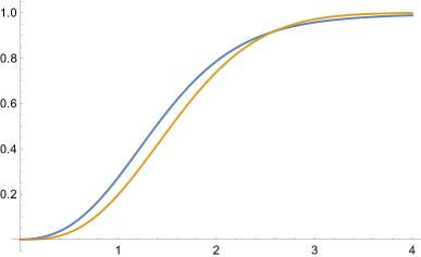
Figure 1: Graphs of $H_{15}$ (blue) and $H$.

Theorem 2.3.

If $F=F_{0}$, then

$$\mathbb{P}(\sqrt{n}V_{n}^{*}\leq x)\rightarrow G(x),$$

where

$$G(x)=$$

$$16\sum_{0\leq j<l<\infty}(-1)^{j+l}\frac{\alpha_{j}\alpha_{l}}{\alpha_{l}^{2}-\alpha_{j}^{2}}[\frac{\Phi(\alpha_{j}x)-1/2}{\alpha_{j}}-\frac{\Phi(\alpha_{l}x)-1/2}{\alpha_{l}}]+\hskip 116.65646pt$$

$$4\sum_{0\leq j<\infty}[\frac{\Phi(\alpha_{j}x)-1/2}{\alpha_{j}}-x\varphi(\alpha_{j}x)],\quad x\geq 0.$$

Here, $\alpha_{j}=2j+1,j\in\mathbb{N}_{0},$ and $\varphi$ denote the density of $N(0,1)$.

Proof.

Observe that $\sqrt{n}W_{n}^{*}=h\circ L(|\alpha_{n}|)$ and $|\alpha_{n}|\stackrel{{\scriptstyle\mathcal{D}}}{{\rightarrow}}|B|$ in $(D[0,1],s)$. Thus the CMT guarantees that

$$\sqrt{n}W_{n}^{*}\stackrel{{\scriptstyle\mathcal{D}}}{{\rightarrow}}h(M(|B|),a(|B|))=:Z$$

and the assertion follows from Theorem 1.1 of Ferger (2018). ∎

3 Power investigations

Recall that $H_{n}(x):=\mathbb{P}(\sqrt{n}W^{*}_{n}\leq x)$ is given by Theorem 2.1. Similarly, for $I_{n}(x):=\mathbb{P}(\sqrt{n}M_{n}(x)\leq x)$ there is an explicit expression according to (2). Finally, $J_{n}(x):=\mathbb{P}(T^{+}_{n}(w)\leq x)$ can be computed via (14)-(16). For a given level $\alpha$ of significance let $z_{\alpha,n},u_{\alpha,n}$ and $y_{\alpha,n}$ be the exact critical values of our test, the Smirnov-test and the MS-test, respectively. Thus these values are determined through $H_{n}(z_{\alpha,n})=I_{n}(u_{\alpha,n})=J_{n}(y_{\alpha,n})=1-\alpha$. For $\alpha=0.05$ we provide a table of the critical values for some selected sample sizes $n$. As to $T^{+}_{n}(w)$ recall that by (13) the weight $w=w_{\alpha}=0.024205$.

Table 1: Exact critical values for $\alpha=0.05$

$n$	$z_{\alpha,n}$	$u_{\alpha,n}$	$y_{\alpha,n}$
30	2.83457	1.19214	1.27950
50	2.81185	1.20014	1.28827
100	2.79586	1.20856	1.29575
500	2.78631	1.21612	1.30498
1.000	2.78484	1.21869	1.30680
10.000	2.79339	1.22238	1.31094
$\infty$	2.79548	1.22387	1.42782

Table 1 shows that the asymptotic critical values of our new test (N-test) and the S-Test are fairly good even for small sample sizes, whereas the asymptotic value of the MS-Test is significantly larger than the exact values even for very large $n$. This indicates that the speed of convergence in (12) seems to be rather slow.

Next we present the results of a small simulation study. Here we choose $F_{0}(x)=x$ on $[0,1]$ and $F=F_{\tau,\delta}$ as in Example 1, that means the alternative $F$ on $[0,1]$ is the simple polygonal line through the points $(0,0),(\tau,\delta\tau))$ and $(1,1)$. We fix $\tau=0.05$ and shortly write $F_{\delta}:=F_{0.05,\delta}$. For $\delta\in[1,1/\tau)=[1,20)$ let

$$\beta^{(N)}_{n}(\delta) :=\mathbb{P}_{\delta}(\sqrt{n}W^{*}_{n}>z_{\alpha,n}),$$

$$\beta^{(S)}_{n}(\delta) :=\mathbb{P}_{\delta}(\sqrt{n}M_{n}>u_{\alpha,n}),$$

$$\beta^{(MS)}_{n}(\delta) :=\mathbb{P}_{\delta}(T^{+}_{n}(w)>y_{\alpha,n})$$

be the power-functions of the N-, S- and MS-test. (Under $\mathbb{P}_{\delta}$ the data $X_{1},\ldots,X_{n}$ are i.i.d. with distribution function $F_{\delta}$). A Monte-Carlo simulation with $10^{4}$ replicates per grid-point yields the following results as displayed in Figure 2-4. Here, the power functions $\beta^{(N)}_{n},\beta^{(S)}_{n}$ or $\beta^{(MS)}_{n}$ are represented by the blue, orange or green line, respectively. We see that for small (n=30), middle (n=100) and large (n=500) sample sizes the $N$-test with a clear distance is uniformly better than the $S$-test, which in turn is uniformly better than the $MS$-test. The latter may come as a surprise, but it may be because of that the weighting by $1/F_{0}(x)$ and $1/(1-F_{0}(x))$ is unduly.

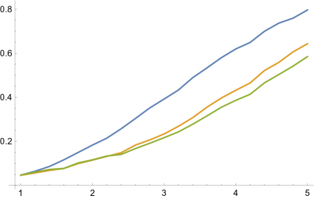
Figure 2: Power for $n=30$

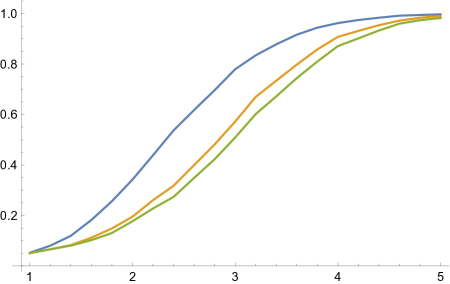
Figure 3: Power for $n=100$

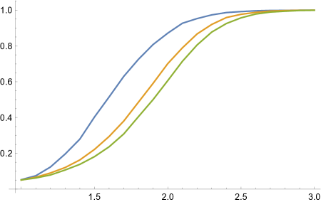
Figure 4: Power for $n=500$

In practical applications the statistician computes the $p$-value. For a given realization of the test-statistics $\sqrt{n}W^{*}_{n},\sqrt{n}M_{n}$ and $T^{+}_{n}(w)$ the corresponding $p$-values are the (random) quantities $1-H_{n}(\sqrt{n}W^{*}_{n}),1-I_{n}(\sqrt{n}M_{n})$ and $1-J_{n}(T^{+}_{n}(w))$.

Appendix

If $F=F_{0}$, then our statistics have the shape

$$W_{n}^{*} =\frac{\frac{R}{n}-F(X_{R:n})}{\sqrt{F(X_{R:n})(1-F(X_{R:n}))}}\quad\text{ with }$$ (18)

$$R =\raisebox{-5.12149pt}{${{\displaystyle\rm arg\,\!max}\atop{\scriptstyle 1\leq i\leq n}}$}\frac{i}{n}-F(X_{i:n})$$ (19)

and

$$V_{n}^{*} =\frac{\max\{\frac{r}{n}-F(X_{r:n}),F(X_{r:n})-\frac{r-1}{n}\}}{\sqrt{F(X_{r:n})(1-F(X_{r:n}))}}\quad\text{ with }$$ (20)

$$r =\raisebox{-5.12149pt}{${{\displaystyle\rm arg\,\!max}\atop{\scriptstyle 1\leq i\leq n}}$}\max\{\frac{i}{n}-F(X_{i:n}),F(X_{i:n})-\frac{i-1}{n}\}.$$ (21)

Lemma .1.

If $F$ is continuous, then the distribution of $W_{n}^{*}$ in (18) does not depend on $F$. The same holds for $V_{n}^{*}$ in (20).

Proof.

By the quantile-transformation we can w.l.o.g. assume that $X_{i}=F^{-1}(U_{i}),1\leq i\leq n$. By continuity of $F$ it follows that $X_{i:n}=F^{-1}(U_{i:n})$ for all indices $i$ and in particular $X_{R:n}=F^{-1}(U_{R:n})$. As in the proof of Lemma A.2 in Ferger (2005) one shows that $R=\raisebox{-5.12149pt}{${{\displaystyle\rm arg\,\!max}\atop{\scriptstyle 1\leq i\leq n}}$}\frac{i}{n}-U_{i:n}$. Since by continuity $F\circ F^{-1}$ is the identity map we obtain from (18) and (19) that

$$W_{n}^{*}=\frac{\frac{R}{n}-U_{R:n}}{U_{R:n}(1-U_{R:n})}\quad\text{ with }\quad R=\raisebox{-5.12149pt}{${{\displaystyle\rm arg\,\!max}\atop{\scriptstyle 1\leq i\leq n}}$}\frac{i}{n}-U_{i:n}.$$

In the same manner one shows that

$$V_{n}^{*} =\frac{\max\{\frac{r}{n}-U_{r:n},U_{r:n}-\frac{r-1}{n}\}}{\sqrt{U_{r:n})(1-U_{r:n})}}\quad\text{ with }$$ (22)

$$r =\raisebox{-5.12149pt}{${{\displaystyle\rm arg\,\!max}\atop{\scriptstyle 1\leq i\leq n}}$}\max\{\frac{i}{n}-U_{i:n},U_{i:n})-\frac{i-1}{n}\}$$ (23)

and the proof is complete. ∎

Lemma .2.

For every $f\in D[0,1]$ let $M(f):=\sup_{t\in[0,1]}f(t)$ and $A(f):=\{t\in[0,1]:\max\{f(t),f(t-)\}=M(f)\}$ with the convention $f(0-):=f(0)$. Then $A(f)$ is non-empty and compact. In particular, $a(f):=\min A(f)$ is well-defined. The statements remain true if $[0,1]$ is replaced by any compact subinterval.

Proof.

Introduce $\bar{f}(x):=\max\{f(x),f(x-)\}$. Then by Lemmas 2.1 and 2.2 of Ferger (2015) the function $\bar{f}$ is the upper semicontinuous regularization of $f$ and $A(f)$ is equal to the set of all maximizing points of $\bar{f}$. Since $[0,1]$ is compact the latter set set is known to be non-empty and compact. ∎

Lemma .3.

The functional $L:=(M,a):(D[0,1],s)\rightarrow\mathbb{R}^{2}$ is Borel-measurable.

Proof.

Since the Borel-$\sigma$ algebra $\mathcal{B}(\mathbb{R}^{2})$ is equal to $\mathcal{B}(\mathbb{R})\otimes\mathcal{B}(\mathbb{R})$ it suffices to show that $M$ and $a$ are Borel-measurable. By right-continuity of $f\in D[0,1]$ we have that $M(f)=\sup_{t\in[0,1]\cap\mathbb{Q}}f(t)$ and therefore $M:(D[0,1],s)\rightarrow\mathbb{R}$ is Borel-measurable upon noticing that the Borel-$\sigma$ algebra on $(D[0,1],s)$ is generated by the projections (evaluation maps), see Theorem 12.5 in Billingsley (1999).

As to measurability of $a$ let $x\in[0,1]$. Then (with $D:=D[0,1])$ we have that

$$\{f\in D:a(f)\leq x\} =\{f\in D:\sup_{t\in[0,x]}f(t)\geq\sup_{t\in[x,1]}f(t)\}$$ (24)

$$=\{f\in D:\sup_{t\in[0,x]\cap\mathbb{Q}}f(t)\geq\sup_{t\in[x,1]\cap\mathbb{Q}}f(t)\}.$$ (25)

To see the equality (24) assume that $a(f)\leq x$, but $\sup_{t\in[0,x]}f(t)<\sup_{t\in[x,1]}f(t)$. Put $\tau:=a(f)$. Then $f(\tau)\leq\sup_{t\in[0,x]}f(t)<\sup_{t\in[x,1]}f(t)\leq M(f)$. If $\tau>0$ we find a sequence $(s_{k})$ with $0<s_{k}\uparrow\tau$, whence $f(\tau-)=\lim_{k\rightarrow\infty}f(s_{k})$. In particular $s_{k}\leq\tau\leq x$ and so $f(s_{k})\leq\sup_{t\in[0,x]}f(t)$ for each $k$. Taking the limit $k\rightarrow\infty$ yields $f(\tau-)\leq\sup_{t\in[0,x]}f(t)<\sup_{t\in[x,1]}f(t)\leq M(f)$. As a consequence $\max\{f(\tau),f(\tau-)\}<M(f)$, a contradiction to $\tau$ is a supremizing point. If $\tau=0$, then by convention $f(0-)=f(0)$ and $f(0)<M(f)$ as seen above. So we arrive at a contradiction also in this case.

For the other direction observe that $M(f)=\max\{\sup_{t\in[0,x]}f(t),\sup_{t\in[x,1]}f(t)\}=\sup_{t\in[0,x]}f(t)=\max\{f(\sigma),f(\sigma-)\}$ for some $\sigma\in[0,x]$ by Lemma .2. Thus $\sigma\in A(f)$ and since $a(f)$ is the smallest supremizing point it follows that $a(f)\leq\sigma\leq x$ as desired. This shows equality (24). The second equality (25) holds, because the respective suprema coincide by right-continuity of $f$. Measurability now follows again by noticing that the Borel-$\sigma$ algebra on $(D[0,1],s)$ is generated by the projections. ∎

Lemma .4.

The argmax-functional $a:(D[0,1],s)\rightarrow[0,1]$ is continuous on the class $C_{u}$ of all continuous functions $f:[0,1]\rightarrow\mathbb{R}$ with unique maximizing point.

Proof.

Let $f\in C_{u}$ with unique minimizer $\tau=a(f)$ and let $(f_{n})$ be a sequence in $D[0,1]$ such that $s(f_{n},f)\rightarrow 0$. Since $f$ is continuous we have that in fact

$$||f_{n}-f||=\sup_{0\leq t\leq 1}|f_{n}(t)-f(t)|\rightarrow 0.$$ (26)

Assume that $\tau\in(0,1)$. For an arbitrary $0<\epsilon\leq\tau\wedge(1-\tau)$ introduce $U_{\epsilon}:=(\tau-\epsilon,\tau+\epsilon]\subseteq[0,1]$ with non-empty complement $V_{\epsilon}=[0,1]\setminus U_{\epsilon}=[0,\tau-\epsilon]\cup(\tau+\epsilon,1]$. Consider

$$m_{\epsilon}:=\sup\{f(t):t\in V_{\epsilon}\}=\sup\{f(t):t\in\bar{V_{\epsilon}}\},$$

where $\bar{V_{\epsilon}}$ is the closure of $V_{\epsilon}$ and equal to $[0,\tau-\epsilon]\cup[\tau+\epsilon,1]$. Here the second equality holds by continuity of $f$. Put $\delta_{\epsilon}:=\frac{1}{3}(f(\tau)-m_{\epsilon})$. Then $\delta_{\epsilon}>0$, because otherwise $f(\tau)=m_{\epsilon}=f(\sigma)$ for some $\sigma\in\bar{V_{\epsilon}}$ upon noticing that $\bar{V_{\epsilon}}$ is compact. Consequently, $\sigma$ is a maximizing point, which differs from $\tau$, because it does not lie in $(\tau-\epsilon,\tau+\epsilon)$. This is a contradiction to the uniqueness of $\tau$. Infer from (26) that there exists a natural number $n_{0}(\epsilon)$ such that

$$||f_{n}-f||\leq\delta_{\epsilon}\quad\forall\;n\geq n_{0}(\epsilon).$$ (27)

Let $t\notin U_{\epsilon}$, so $t\in V_{\epsilon}$. Notice that

$$f_{n}(\tau)-f_{n}(t)=[f_{n}(\tau)-f(\tau)]+[f(\tau)-f(t)]+[f(t)-f_{n}(t)].$$ (28)

By (27) the first summand $f_{n}(\tau)-f(\tau)$ and the third summand $f(t)-f_{n}(t)$ are greater or equal $-\delta_{\epsilon}$. As to the second summand observe that $f(t)\leq m_{\epsilon}$, because $t\in V_{\epsilon}$. Thus $f(\tau)-f(t)\geq f(\tau)-m_{\epsilon}=3\delta_{\epsilon}$. Summing up we arrive at $f_{n}(\tau)-f_{n}(t)\geq-2\delta_{\epsilon}+3\delta_{\epsilon}=\delta_{\epsilon}$ or equivalently

$$f_{n}(t)\leq f_{n}(\tau)-\delta_{\epsilon}<f_{n}(\tau)\quad\forall\;t\notin U_{\epsilon}\quad\forall\;n\geq n_{0}(\epsilon).$$ (29)

From this basic inequality we can derive that also

$$f_{n}(t-)<f_{n}(\tau)\quad\forall\;t\notin U_{\epsilon}\quad\forall\;n\geq n_{0}(\epsilon).$$ (30)

To see this consider at first the case $t\in(0,\tau-\epsilon]$. Then there exists a sequence $(s_{k})$ with $0<s_{k}\uparrow t$, whence by (29) applied to $t=s_{k}$ it follows that $f_{n}(t-)=\lim_{k\rightarrow\infty}f_{n}(s_{k})\leq f_{n}(\tau)-\delta_{\epsilon}<f_{n}(\tau)$. In the same way one can treat the case $t\in(\tau+\epsilon,1]$ and finally if $t=0$, then $f_{n}(0-)=f_{n}(0)$ by definition and another application of (29) gives (30). Now, (29) and (30) show that

$$\max\{f_{n}(t),f_{n}(t-)\}<f_{n}(\tau)\quad\forall\;t\notin U_{\epsilon}\quad\forall\;n\geq n_{0}(\epsilon).$$ (31)

Conclude that

$$\tau_{n}:=a(f_{n})\in U_{\epsilon}\quad\forall\;n\geq n_{0}(\epsilon),$$ (32)

because otherwise there exists an $n\geq n_{0}(\epsilon)$ such that $\tau_{n}\notin U_{\epsilon}$. But since $\tau_{n}$ is the (smallest) supremizing point of $f_{n}$ we obtain with (31) that $M(f_{n})=\max\{f_{n}(\tau_{n}),f_{n}(\tau_{n}-)\}<f_{n}(\tau)$, a contradiction to $M(f_{n})$ is the (least) upper bound of $f_{n}$. In the extreme cases $\tau=0$ or $\tau=1$ one considers $U_{\epsilon}$ equal to $[0,\epsilon]$ or $(1-\epsilon,1]$, respectively, and the same modus operandi as above leads to (32). Thereby we have shown that $a(f_{n})\rightarrow a(f)$ whenever $f_{n}\rightarrow_{s}f$, which means that $a$ is continuous at $f$. ∎

References

• Anderson and Darling (1952) Anderson, T. W. and Darling, D. A. (1952). Asymptotic theory of certain ”goodness of fit criteria based on stochastic processes. Ann. Math. Statist., 23, 193–212.
• Billingsley (1999) Billingsley, P. (1999). Convergence of Probability Measures, 2nd ed. New York: Wiley.
• Birnbaum (1958) Birnbaum, Z. W. and Pyke, R. (1958). On some distributions related to the statistic $D_{n}^{+}$. Ann. Math. Statist., 29, 179–187.
• Cahill et. al. (2002) Cahill, N. D., D’Errico, J. R., Narayan, D. A. and Narayan, J. Y. (2002). Fibonacci Determinants. The College Mathematics Journal, 33, 221–225. DOI: 10.1080/07468342.2002.11921945
• Chang (1955) Chang, L. C. (1955). On the ratio of the empirical distribution to the theoretical distribution function. Acta Math. Sinica, 5, 347–368. (English translation in Selected Transl. Math. Statist. Prob., 4 (1964), 17–38.)
• Chibisov (1966) Chibisov, M. D. (1966). Some theorems on the limiting behavior of the empirical distribution function. Selected Translations Math. Statist. Prob, 6, 147-156.
• Csörgő and Horváth (1993) Csörgő, M. and Horváth, L. (1993). Weighted Approximations in Probability and Statistics, Chichester, England: Wiley.
• Daniels (1945) Daniels, H. E. (1945). The statistical theory of the strength of bundles of threads. Proc. Roy. Soc. London Ser. A, 183, 405–435.
• Ferger (2005) Ferger, D. (2005). On the minimizing point of the incorrectly centered empirical process and its limit distribution in nonregular experiments. ESAIM: Probability and Statistics, 9, 307-322.
• Ferger (2015) Ferger, D. (2015). Arginf-sets of multivariate cadlag processes and their convergence in Hyperspace topologies. Theory of Stochastic Processes, 20 (36), 13–41.
• Ferger (2018) Ferger, D. (2018). On the supremum of a Brownian bridge standardized by its maximizing point with applications to statistics. Statist. Probab. Lett., 134, 63–69.
• Gänsler and Stute (1977) Gänsler, P. and Stute, W. (1977). Wahrscheinlichkeitstheorie, Berlin, Heidelberg: Springer.
• Gutjahr (1988) Gutjahr, M. (1988). Zur Berechnung geschlossener Ausdrücke für die Verteilung von Statistiken, die auf einer empirischen Verteilungsfunktion basieren, Phd-thesis, Ludwig-Maximilians-University, München.
• Ishii (1959) Ishii, G. (1959). On the exact probabilities of Rényi’s tests. Ann. Inst. Statist. Math. Tokyo, 11, 17–24.
• Jaeschke (1979) Jaeschke, D. (1979). The asymptotic distribution of the supremum of the standardized empirical distribution function on subintervals. Ann. Statist., 7, 108–115.