Structure-preserving finite-element schemes for the Euler-Poisson equations

Abstract

We discuss structure-preserving numerical discretizations for repulsive and attractive Euler-Poisson equations that find applications in fluid-plasma and self-gravitation modeling. The scheme is fully discrete and structure preserving in the sense that it maintains a discrete energy law, as well as hyperbolic invariant domain properties, such as positivity of the density and a minimum principle of the specific entropy. A detailed discussion of algorithmic details is given, as well as proofs of the claimed properties. We present computational experiments corroborating our analytical findings and demonstrating the computational capabilities of the scheme.

65M22, 35L65, 35Q31

1 Introduction

In this manuscript we develop numerical schemes for the repulsive and attractive Euler-Poisson equations. This is a system of equations that combine the hyperbolic compressible Euler equations of gas dynamics that describe the time evolution of a fluid state (consisting of pressure, momentum and total energy) with the action of a scalar potential that in turn depends on the time evolution of the density of the system. The Euler-Poisson equations have found applications in the context of plasma physics [56], semiconductor device modeling [51], and vacuum electronics [67]. The equations are often used to model an electron fluid subject to electrostatic forces. The Euler-Poisson system is also routinely used in astrophysics [57] for modeling large scale formation of galaxies due to self-gravitation.

Our goal is to develop a numerical method for the Euler-Poisson system that is second order accurate and provably robust. By this we mean that the fully discrete update procedure at each time-step is locally well-posed, implying: (a) that the numerical scheme is always able to compute a new admissible state (i. e., with positive density and internal energy); (b) it preserves a discrete energy law; and (c) that the linear algebra only involves symmetric positive definite problems, while the time-step size is only subject to a hyperbolic CFL condition. Our approach is based on an operator splitting in order to decouple the hyperbolic and elliptic subsystems. We consider a fully-discrete analysis of the scheme, revealing the need of specific choices of space and time discretization that we make precise in Section 3.

The splitting approach allows us to relegate invariant domain preservation entirely to the numerical scheme used for the hyperbolic system; see Section 2. This leaves considerable freedom for the specific choice of hyperbolic solver. In particular, one could choose a numerical method that preserves all invariant sets, or a subset of the invariant set properties, such as positivity of density and internal energy, see [37, 42]. The resulting scheme will be invariant domain preserving if the hyperbolic solver preserves all invariants. For the sake of completeness we briefly describe the hyperbolic solver used in this manuscript in Appendix A.

1.1 The Euler-Poisson system

We consider a general model problem derived by coupling the compressible Euler equations of gas dynamics to a scalar potential:

(1a) $$\partial_{t}\rho+\text{div}\,\mathbf{}\mathbf{m} =0,$$

(1b) $$\partial_{t}\mathbf{m}+\text{div}\,\mathbf{}\big{(}\rho^{-1}\mathbf{m}\mathbf{m}^{\top}+Ip\big{)} =-\rho\nabla\varphi-\frac{1}{\,\uptau}\mathbf{m},$$

(1c) $$\partial_{t}\mathcal{E}+\text{div}\,\mathbf{}\Big{(}\frac{\mathbf{m}}{\rho}(\mathcal{E}+{\rm Phys.\leavevmode\nobreak\ Rev.\leavevmode\nobreak\ E})\Big{)} =-\nabla\varphi\cdot\mathbf{m}-\frac{1}{\rho\,\uptau}|\mathbf{m}|^{2},$$

(1d) $$-\Delta\varphi =\alpha(\rho+\rho_{b}).$$

Here, $\rho(\boldsymbol{x},t)\in\mathbb{R}^{+}$ is the mass density, $\mathbf{m}(\boldsymbol{x},t)\in\mathbb{R}^{d}$, the momentum, $\mathcal{E}(\boldsymbol{x},t)\in\mathbb{R}^{+}$ the total energy, ${\rm Phys.\leavevmode\nobreak\ Rev.\leavevmode\nobreak\ E}\in\mathbb{R}$ denotes the thermodynamic pressure, and $\rho_{b}(\boldsymbol{x},t)\in\mathbb{R}$ denotes a prescribed background density that, in contrast to the mass density $\rho$, might attain negative values. The balance of momentum and total energy equations (1b) and (1c) include a force caused by a scalar potential $\varphi(\boldsymbol{x},t)$ whose time evolution in turn is coupled to the density $\rho(\boldsymbol{x},t)$ of the system. The model includes a relaxation term $-\tfrac{1}{\,\uptau}\mathbf{m}$ in the momentum equation where $\,\uptau>0$ is a so-called relaxation time of the system. For example, this could model resistive or collisional effects with an electrically neutral species. By slight abuse of notation we set $\,\uptau=+\infty$ for the case of a vanishing relaxation effects. In case of a positive coupling constant, $\alpha>0$, system (1) is said to be repulsive, meaning, the force term $-\rho\nabla\varphi$ in (1b) repels density accumulations. The corresponding case of a negative coupling constant, $\alpha<0$, leads to an attractive system (1) where density accumulations attract each other. We close system (1) by prescribing a simple polytropic equation of state where the pressure follows the ideal gas law, i. e., $p=(\gamma-1)(\mathcal{E}-\frac{1}{2}\rho^{-1}|\mathbf{m}|_{\ell^{2}}^{2})$, with $\gamma=5/3$.

Examples 1.1 and 1.2 illustrate two prototypical applications of the Euler-Poisson equations. Generally speaking, mathematical models describing the dynamics of a “density” subject to its own self-consistent field is a somewhat universal theme in mathematical physics [9, 32, 16, 48]. In this regard, the Euler-Poisson system can be viewed as the simplest prototypical model that contains all necessary mechanisms. Thus, developing and understanding numerical methods for the Euler-Poisson system may open up a path for new ideas and development for other self-consistent models appearing in quantum, molecular, and statistical physics.

Example 1.1 (Electron fluid plasma).

An important example of a repulsive system that can be expressed with (1) is an electron fluid subject to an electrostatic force. Here, $\rho$ takes the meaning of an electron mass density, and $\varphi$ is the electrostatic potential. The coupling constant in this case is given by $\alpha=\frac{1}{\varepsilon_{0}}\frac{q_{e}^{2}}{m_{e}^{2}}$ where $\varepsilon_{0}$ is the vacuum permittivity, $q_{e}$ is the specific electron charge (charge per unit particle), and $m_{e}$ is the specific electron mass (mass per unit particle), $\varphi\in\mathbb{R}$ is the electric potential, and $\,\uptau$ denotes a characteristic collision-time.

Example 1.2 (Euler-Poisson gravity model).

An example of an attractive system is given by an Euler-Poisson gravity model. Here, the density $\rho(\boldsymbol{x},t)$, momentum $\mathbf{m}(\boldsymbol{x},t)$, and total mechanical energy $\mathcal{E}(\boldsymbol{x},t)$ describe the time evolution of the matter of a celestial body subject to self-gravitation. The latter is expressed by the (classical) gravitational potential $\varphi(\boldsymbol{x},t)$ governed by (1d) with the coupling constant

$$\alpha=-4\pi\,G,$$

where $G$ is the graviational constant, and where the relaxation terms have been removed from system (1) by formally setting $\,\uptau=\infty$.

1.2 Structure preservation and stability properties

Developing numerical schemes for the Euler-Poisson system (1) is not a trivial task. It is the authors’ impression that the current body of mathematical literature on the topic for provably robust, fully discrete, self-consistent schemes for the Euler-Poisson system is far from complete at this point in time. In the mathematical literature, the repulsive electrostatic case (of Example 1.1) has been studied by Degond and collaborators [21, 22, 25, 24]. For the attractive gravitational case (Example 1.2) we refer the reader to [66, 45]. It is worth mentioning the astrophysics literature reporting computations of fluids subject to self-gravitational effects is vast. However, precise descriptions of the fully discrete numerical schemes and the mathematical properties guaranteed by such schemes, in general, is not provided. We refer the reader to [65, 1, 61, 15] where schemes used in practice are discussed with some detail.

The fundamental question we wish to pose and examine is: What mathematical properties should a “good” numerical scheme of the Euler-Poisson system possess? To this end we collect a list of desirable properties that the continuous PDE exhibits (at least formally; see Section 2).

We start with two important properties that imply local well-posedness regardless of the numerical scheme of choice. By this we mean that for each time step, the discrete map $\{\rho^{n},\mathbf{m}^{n},\mathcal{E}^{n},\varphi^{n}\}\rightarrow\{\rho^{n+1},\mathbf{m}^{n+1},\mathcal{E}^{n+1},\varphi^{n+1}\}$ is computable:

• Preservation of invariant domain: positivity of the density and pointwise minimum principle of the specific entropy [42, 36]. These conditions ensure that the hyperbolic subsystem is locally well-posed at each time step [42, 36].

• Linear systems arising due to semi-implicit time marching, and their discretization in space, shall be well-posed for all physically admissible regimes, meaning that: all linear systems are invertible and/or do not exhibit any artificial rank-deficiency.

Properties (i) and (ii) ensure that all discrete subsystems of our numerical scheme are well-posed. Assuming these conditions are met, we can pursue additional properties that the local map $\{\rho^{n},\mathbf{m}^{n},\mathcal{E}^{n},\varphi^{n}\}\rightarrow\{\rho^{n+1},\mathbf{m}^{n+1},\mathcal{E}^{n+1},\varphi^{n+1}\}$ should preserve:

• Satisfaction of a discrete total-energy balance.

• Preservation of the Hamiltonian structure of the source-dominated regime; see Remark 2.8 in Section 2.3.

• Satisfaction of a discrete Gauß law (1d) at the end of each time-step.

In addition a number of discrete properties arise from enforcing compatibility with limiting equations [52, 21, 22, 46], in particular in the repulsive case ($\alpha>0$). The numerical scheme:

• Should not require to resolve the electrostatic plasma-oscillation time-scale (see Remark 2.7 in Section 2.3); or at least the plasma-oscillation should not be a source of numerical instabilities in the scheme [52].

• Should be asymptotic-preserving with respect to the quasi-neutral regime [21, 22].

• Should be asymptotic-preserving with respect to the drift-diffusion model. The drift-diffusion model is formally achieved in the zero-relaxation limit ($\,\uptau\rightarrow 0^{+}$), see for instance [46] and references therein.

This is a very ambitious list of desirable mathematical properties for the discrete scheme that, to the best of our knowledge, no single numerical discretization can achieve simultaneously. For instance, we are not aware of any fully discrete numerical scheme satisfying, both, properties (iii) and (v) simultaneously. Similarly, we are not aware of any fully discrete scheme satisfying properties (vii) and (iii) at the same time, and we are not aware of the existence of any self-consistent scheme satisfying (viii). We briefly mention that another very important property is the preservation of steady states. There is indeed a very large body literature on well-balanced schemes for Euler equations with gravitation, see for instance [47, 20] and references therein, but the potential is assumed to be ‘given’ (not computed in a self-consistent manner) in these and related references.

In this manuscript we focus on developing numerical schemes for system (1) for which properties (i)-(iv) can always be guaranteed. We also present a relaxation technique in order to enforce property (v) at the expense of introducing a consistency error in time. In every case the potential is computed self-consistently.

1.3 Background and related literature

System (1) may be understood as a hyperbolic PDE subject to an elliptic constraint (1d). As such it can be reformulated in various different ways [53, 66, 45, 21, 22]. For the sake of discussion we focus on two modifications of the original system (1). First, we can reformulate (1) by rewriting writing the gradient of the potential in nonlocal form, viz. $\nabla\varphi=\alpha\nabla(-\Delta)^{-1}\rho$, and then substituting into the remaining equations of $\eqref{Model}$ thereby eliminating the last equation. This leads to the following nonlocal formulation:

(2a) $$\partial_{t}\rho+\text{div}\,\mathbf{}\mathbf{m} =0,$$

(2b) $$\partial_{t}\mathbf{m}+\text{div}\,\mathbf{}\big{(}\rho^{-1}\mathbf{m}\mathbf{m}^{\top}+Ip\big{)} =\boldsymbol{\mathit{f}}-\frac{1}{\,\uptau}\mathbf{m},$$

(2c) $$\partial_{t}\mathcal{E}+\text{div}\,\mathbf{}\Big{(}\frac{\mathbf{m}}{\rho}(\mathcal{E}+{\rm Phys.\leavevmode\nobreak\ Rev.\leavevmode\nobreak\ E})\Big{)} =\frac{1}{\rho}\boldsymbol{\mathit{f}}\cdot\mathbf{m}-\frac{1}{\rho\,\uptau}|\mathbf{m}|^{2},$$

where we have introduced a force $\boldsymbol{\mathit{f}}:=-\alpha\rho(\nabla(-\Delta)^{-1}(\rho+\rho_{b})$. Clearly, (2) is not any easier to solve than (1). Secondly, equation (1d) can be rewritten as an evolution equation by taking the time derivative and substituting (1a):

(3) $$-\Delta\partial_{t}\varphi =-\alpha\,\text{div}\,\mathbf{}\mathbf{m}\;+\;\alpha\partial_{t}\rho_{b}.$$

In this paper we exploit some aspects of the simplicity of (2), since it can be viewed as just being the Euler equations evolving the triple $[\rho,\mathbf{m},\mathcal{E}]^{\top}$ subject to an external force $\boldsymbol{\mathit{f}}$; see Section 2. We also use the time dependent formulation (3) of the potential in order to avoid any kind of numerical non-locality in the resulting hyperbolic scheme. This allows us to develop a numerical scheme satisfying properties (i)–(iv). We also present a relaxation technique in order to address property (v)—the preservation of a discrete Gauß law—which may introduce some purely numerical dissipation into the total energy-balance.

Remark 1.3.

It is certainly possible to reformulate system (1) even further. A number of variants have been explored in the literature in this regard. For example, one approach is to rewrite the source terms containing $\rho\nabla\varphi$ in divergence-form leading to a nonlocal conservation law with fluxes that are nonlocal in space and time [53, 66, 45]:

$$\partial_{t}\rho+\text{div}\,\mathbf{}\mathbf{m} =0,$$

(4) $$\partial_{t}\mathbf{m}+\text{div}\,\mathbf{}\Big{(}\rho^{-1}\mathbf{m}\mathbf{m}^{\top}+Ip+\alpha^{-1}(\nabla\varphi\nabla\varphi^{\top}-\tfrac{1}{2}|\nabla\varphi|^{2}\mathbb{I})\Big{)} =-\frac{1}{\,\uptau}\mathbf{m},$$

$$\partial_{t}E+\text{div}\,\mathbf{}\Big{(}\frac{\mathbf{m}}{\rho}(E+{\rm Phys.\leavevmode\nobreak\ Rev.\leavevmode\nobreak\ E})+\frac{1}{2\alpha}(\varphi\nabla\partial_{t}\varphi-\partial_{t}\varphi\nabla\varphi)\Big{)} =-\frac{1}{\rho\,\uptau}|\mathbf{m}|^{2}.$$

with $E=\mathcal{E}+\frac{1}{2}\rho\varphi=\mathcal{E}+\frac{1}{2\alpha}|\nabla\varphi|^{2}$. The conservation law structure is indeed interesting, but it has to be noted that such nonlocal fluxes have very different mathematical properties from those found for example for the Euler equations. This leads to a number of difficulties that can call to question the benefits of this approach. Most importantly, the force $\boldsymbol{\mathit{f}}:=-\alpha\rho(\nabla(-\Delta)^{-1}(\rho+\rho_{b}))$, even if rewritten in divergence-form, exhibits an infinite speed of propagation: in this context the new balance law is unlikely to be hyperbolic. This is a roadblock if we want to guarantee robustness, as it would require to develop either a Godunov-type solver or at the very least finding a guaranteed estimate of the maximum wavespeed across the Riemann fan [64, 39, 42, 63]. This is problematic, since the maximum wavespeed across the Riemann fan is, by construction, infinite in this context. We are not the first ones to point-out related concerns, see for instance [59, p. 48].

Even if the issues mentioned above can be properly addressed, on a practical note, the discrete counterparts of the nonlocal fluxes in system (4) exhibit a scaling of the form $\mathcal{O}(h^{-2})$ where $h$ denotes the mesh size. This poses the issue that explicit time-marching (which we are using) might then be subject to a parabolic CFL condition of the form $\tau\sim h^{2}$.

Remark 1.4.

A different approach one could pursue is to follow the steps of the pioneering work of [21, 22] on asymptotic-preserving schemes in the quasi-neutral regime (Property (vi) discussed in Section 1.2). Such approaches, however, require major commitment to semi-implicit time integration of the hydrodynamical subsystem. A situation for which—to the best of our knowledge—rigorously guaranteeing invariant domain preservation is a challenging and open mathematical problem; see [54, 71, 42] and references therein.

In particular, there are no general-purpose time-implicit schemes for nonlinear hyperbolic systems of conservation laws with mathematical guarantees of local solvability and pointwise stability for the shock-hydrodynamics regime. This is particularly important if we are interested in the full-Euler system and not just barotropic models. Progress in this direction can be found in [44, 18, 8, 62, 23].

Finally, in the vast majority of references presenting computations and/or schemes for Euler-Poisson system, see for instance [21, 22, 25, 24, 53, 66, 45, 65, 1, 61, 15] and references therein, the primary space discretization techniques are finite volumes for the hyperbolic sub-system, and either finite differences and/or integral methods for the elliptic operators, in cartesian meshes. However, during the last two decades, there has been an explosive growth of versatile finite element frameworks/libraries, see for instance [4, 5, 2, 3], capable of supporting a large number of space-discretizations, linear solvers, preconditioners, and adaptivity among many other features. There has also been significant development of collocation methods that can solve hyperbolic systems of conservation laws [37, 42] using finite-element infrastructure while also providing mathematically guaranteed robustness. In this sense the current work is a significant point of departure from pre-existing literature: we present new schemes that are meant to be coded entirely within the scope of a finite element library. In particular, we use the finite element library deal.II [4, 5] and exploit the mathematical framework of numerical schemes for hyperbolic systems of conservation laws developed in [42].

1.4 Paper organization

The remainder of the paper is organized as follows. We discuss fundamental (formal) stability properties of the continuous PDE and limits of the PDE in Section 2. The discretization approach of our numerical scheme is discussed in Section 3. Section 4 introduces postprocessing strategies to maintain the discrete Gauß law. Section 5 presents computational results that illustrate the properties of the proposed numerical schemes. We conclude with a short summary and outlook in Section 6.

2 Fundamental stability properties

In preparation for Sections 3 and 4 in which structure-preserving numerical schemes are introduced, we first discuss some fundamental stability properties of the PDE. We start with the Euler equations without source terms and then proceed to the system (2) and (3).

2.1 Euler equations with forces

We start by collecting a number of useful properties of the solution $\mathbf{u}:=[\rho,\mathbf{m},\mathcal{E}]^{T}$ of (2) when fixing the force $\mathbf{f}$ and in the case of no relaxation, i. e., $\,\uptau=\infty$. In order to simplify notation we rewrite (2) in compact form as follows:

(5) $$\frac{\partial}{\partial t}\mathbf{u}+\text{div}\,\mathbf{}\boldsymbol{\mathbb{f}}(\mathbf{u})=\mathbf{s}(\mathbf{f}),$$

where

(6) $$\boldsymbol{\mathbb{f}}(\mathbf{u})=\begin{bmatrix}\mathbf{m}^{\top}\\ \rho^{-1}\mathbf{m}\mathbf{m}^{\top}+Ip\\ \rho^{-1}\mathbf{m}^{\top}(\mathcal{E}+p)\end{bmatrix},\qquad\mathbf{s}(\mathbf{f})=\begin{bmatrix}0\\ \mathbf{f}\\ \rho^{-1}\mathbf{m}\cdot\mathbf{f}\end{bmatrix}.$$

Here, deviating from Section 1.3, the force density $\mathbf{f}:=\mathbf{f}(\boldsymbol{x},t):\mathbb{R}^{d}\times\mathbb{R}\rightarrow\mathbb{R}^{d}$ shall be an arbitrary prescribed vector field possibly depending on the state $\mathbf{u}$, the space $\boldsymbol{x}$ and time $t$. Note that $\rho^{-1}\mathbf{m}\cdot\mathbf{f}$, acting on the energy equation, is the power of the force $\mathbf{f}$ per unit volume.

Lemma 2.1 (Tangent-in-time invariance of the density and internal energy).

Let $\Psi(\mathbf{u}):\mathbb{R}^{d+2}\rightarrow\mathbb{R}$ be any arbitrary functional of the state satisfying the functional dependence $\Psi(\mathbf{u}):=\psi(\rho,\varepsilon(\mathbf{u}))$ where $\varepsilon(\mathbf{u}):=\mathcal{E}-\frac{|\mathbf{m}|^{2}}{2\rho}$ is the internal energy per unit volume. Then we have that

(7) $$\nabla_{\mathbf{u}}\Psi(\mathbf{u})\cdot\mathbf{s}(\mathbf{f})\equiv 0,$$

where $\nabla_{\mathbf{u}}$ is the gradient with respect to the state, i. e., $\nabla_{\mathbf{u}}=\big{[}\frac{\partial}{\partial\rho},\frac{\partial}{\partial\mathbf{m}_{1}},...,\frac{\partial}{\partial\mathbf{m}_{d}},\frac{\partial}{\partial\mathcal{E}}\big{]}^{\top}$.

Proof 2.2.

Using the chain rule we observe that $\nabla_{\mathbf{u}}\Psi(\mathbf{u})=\frac{\partial\psi}{\partial\rho}\nabla_{\mathbf{u}}\rho+\frac{\partial\psi}{\partial\varepsilon}\nabla_{\mathbf{u}}\varepsilon$, where

$$\nabla_{\mathbf{u}}\rho =[1,0,...,0]^{\top}\in\mathbb{R}^{d+2},$$

$$\nabla_{\mathbf{u}}\varepsilon =\Big{[}\frac{|\mathbf{m}|^{2}}{\rho^{2}},-\frac{\mathbf{m}_{1}}{\rho},...,-\frac{\mathbf{m}_{d}}{\rho},1\Big{]}^{\top}\in\mathbb{R}^{d+2}.$$

Taking the product with $\mathbf{s}(\mathbf{f})$ we get

$$\nabla_{\mathbf{u}}\Psi(\mathbf{u})\cdot\mathbf{s}(\mathbf{f}) =\frac{\partial\psi}{\partial\rho}\underbrace{\nabla_{\mathbf{u}}\rho\cdot\mathbf{s}(\mathbf{f})}_{=\,0}+\frac{\partial\psi}{\partial\varepsilon}\nabla_{\mathbf{u}}\varepsilon\cdot\mathbf{s}(\mathbf{f})$$

$$=\frac{\partial\psi}{\partial\varepsilon}(-\rho^{-1}\mathbf{m}\cdot\mathbf{f}+\rho^{-1}\mathbf{m}\cdot\mathbf{f})=0.$$

Remark 2.3 (Colloquial interpretation).

Lemma 2.1 is simply saying that the evolution in time of an arbitrary functional of the state $\Psi(\mathbf{u})$ satisfying the functional dependence $\Psi(\mathbf{u}):=\psi(\rho,\varepsilon(\mathbf{u}))$ is independent of the force $\mathbf{f}$. This follows directly by taking the dot-product of (5) with $\nabla_{\mathbf{u}}\Psi(\mathbf{u})$ to get

$$\nabla_{\mathbf{u}}\Psi(\mathbf{u})\cdot\tfrac{\partial}{\partial t}\mathbf{u}\;=\;\tfrac{\partial}{\partial t}\Psi(\mathbf{u})\;=\;-\nabla_{\mathbf{u}}\Psi(\mathbf{u})\cdot\text{div}\,\mathbf{}\boldsymbol{\mathbb{f}}(\mathbf{u})+\underbrace{\nabla_{\mathbf{u}}\Psi(\mathbf{u})\cdot\mathbf{s}(\mathbf{f})}_{\equiv\,0}.$$

In particular, this holds true when $\Psi(\mathbf{u}):=\varepsilon(\mathbf{u})$. Similarly, we can apply Lemma 2.1 to the specific internal energy $e(\mathbf{u})=\rho^{-1}\varepsilon(\mathbf{u})$ since $e(\mathbf{u})$ satisfies the functional dependence $e(\mathbf{u})=\psi(\rho,\varepsilon(\mathbf{u}))$ as well.

Lemma 2.1 and Remark 2.3 lead us to the following immediate corollary.

Corollary 2.4.

Let $\sigma(\rho,e(\mathbf{u}))$ denote the specific internal entropy, and $\eta(\rho,\sigma)=-\rho\,\sigma(\rho,e(\mathbf{u}))$ denote the mathematical entropy. Then we have that

(8) $$\nabla_{\mathbf{u}}\sigma(\rho,e)\cdot\mathbf{s}(\mathbf{f})\equiv 0\quad\text{therefore}\quad\nabla_{\mathbf{u}}\eta(\rho,\sigma)\cdot\mathbf{s}(\mathbf{f})\equiv 0.$$

The statement follows by using the chain rule, and identity (7) respectively. This implies that forces (more precisely source terms $\mathbf{s}(\mathbf{f})$ as described by expression (6)) can modify neither the specific, nor the mathematical entropy. In this manuscript we are only concerned with the case that $\sigma(\rho,e)=\ln(e^{\frac{1}{\gamma-1}}\rho^{-1})$, which corresponds with the ideal gas closure. However, Corollary 2.4 remains valid for any equilibrium equation of state [43, 38].

2.2 Formal balance equation of the Euler-Poisson system

Lemma 2.5 (Formal balance equation).

For the sake of simplicity let’s assume that $\partial_{t}\rho_{b}\equiv 0$, then the Euler-Poisson system (1) satisfies the formal balance:

(9) $$\frac{\partial}{\partial t}\int_{\Omega}\Big{\{}\mathcal{E}+\frac{1}{2\alpha}|\nabla\varphi|^{2}\Big{\}}\,\mathrm{d}\boldsymbol{x}\;+\;\int_{\partial\Omega}\Big{\{}\frac{\mathbf{m}}{\rho}(\mathcal{E}+p)+\varphi\,\Big{(}\mathbf{m}-\frac{1}{\alpha}\nabla\partial_{t}\varphi\Big{)}\Big{\}}\cdot\boldsymbol{\mathrm{n}}\,\mathrm{d}\boldsymbol{s}\\ \;=\;-\int_{\Omega}\frac{1}{\rho\,\uptau}|\mathbf{m}|^{2}\,\mathrm{d}\boldsymbol{x}.$$

Note that only for the repulsive case $\alpha>0$ the scalar $\{\mathcal{E}+\frac{1}{2\alpha}|\nabla\varphi|^{2}\}$ is an energy density, and thus, Equation (9) represents an energy-flux balance. In case of an attractive Euler-Poisson system, that is $\alpha<0$, the expression $\{\mathcal{E}+\frac{1}{2\alpha}|\nabla\varphi|^{2}\}$ is more closely related to a Lagrangian, the difference of kinetic/total energy and potential energy, see also Definition 2.6.

We call (9) a formal balance equation because it is valid only under the assumption that the solution (as function of time) remains sufficiently integrable in space. The hyperbolic character of (1) poses a fundamental challenge for mathematically deriving such integrability properties. For example, in order for (9) to remain a valid mathematical expression we would want to require that $\nabla\varphi$ remains $L^{2}$-integrable in space. Suppose now that the Gauß law (1d), viz., $-\Delta\varphi=\alpha\rho$, is satisfied for all time, then this requires $\rho\in H^{-1}(\Omega)$. From well-known Sobolev imbedding theorems (see for instance [31, Ch. 5]) we know for instance that $\|\rho\|_{H^{-1}(\Omega)}\lesssim\|\rho\|_{L^{p}(\Omega)}$, provided that $p\geq\frac{6}{5}$ in three spatial dimensions, $d=3$. This means that the density should be $\rho\in L^{p}(\Omega)$ with $p\geq\frac{6}{5}$ in order to guarantee that the $\nabla\varphi$ remains in $L^{2}(\Omega)$. This would be a questionable assumption, since to the best of the authors knowledge, at present it is not possible to guarantee such integrability for the density. Even worse, there is a growing body of scientific literature [50, 17, 26] indicating that finite-time blow-up, i. e., the loss of integrability, indeed happens.

Current mathematical evidence does not align in favor of identity (9). We nevertheless take a pragmatic standpoint in this manuscript and make (an inequality version of) identity (9) a guiding principle for our numerical algorithm development. In this sense (9) should be understood as a regularity assumption that we wish to maintain on the discrete level.

2.3 Asymptotic source dominated regime

In order to simplify some arguments in the following discussion we restrict ourselves to the case of a constant (in time) background density, i. e., $\partial_{t}\rho_{b}\equiv 0$. A generalization of the numerical approach to time-dependent background densities is discussed in Section 3.6.

Definition 2.6 (Source-dominated regime).

The source-dominated regime of the repulsive ($\alpha>0$) Euler-Poisson system (1a)-(1c) and (3) is given by the limiting equations in which all fluxes are set to zero (assuming $\partial_{t}\rho_{b}\equiv 0$):

(10a) $$\partial_{t}\rho =0,$$

(10b) $$\partial_{t}\mathbf{m} =-\rho\nabla\varphi-\frac{1}{\,\uptau}\mathbf{m},$$

(10c) $$\partial_{t}\mathcal{E} =-\nabla\varphi\cdot\mathbf{m}-\frac{1}{\rho\,\uptau}|\mathbf{m}|^{2},$$

(10d) $$-\Delta\partial_{t}\varphi =-\alpha\,\text{div}\,\mathbf{}\mathbf{m}.$$

Note that in (10) only $\mathbf{m}(\boldsymbol{x},t)$ and $\varphi(\boldsymbol{x},t)$ remain as coupled unknowns governed by (10b) and (10d). A direct computation shows that system (10a)-(10c) satisfies the identity $\partial_{t}\big{(}\mathcal{E}-\tfrac{|\mathbf{m}|^{2}}{2\rho}\big{)}\equiv 0$, see also Lemma 2.1. In addition, subsystem (10b)-(10d) satisfies an integral balance equation, viz.,

(11) $$\frac{\partial}{\partial t}\int_{\Omega}\Big{\{}\frac{1}{2\rho}|\mathbf{m}|^{2}+\frac{1}{2\alpha}|\nabla\varphi|^{2}\Big{\}}\,\mathrm{d}\boldsymbol{x}+\int_{\partial\Omega}\Big{\{}\varphi\,\Big{(}\mathbf{m}-\frac{1}{\alpha}\nabla\partial_{t}\varphi\Big{)}\Big{\}}\cdot\boldsymbol{\mathrm{n}}\,\mathrm{d}\boldsymbol{s}\\ \;=\;-\int_{\Omega}\frac{1}{\rho\,\uptau}|\mathbf{m}|^{2}\,\mathrm{d}\boldsymbol{x}.$$

We note in passing that (11) is an energy-flux balance equation only for the repulsive case $\alpha>0$. In case of a negative coefficient $\alpha<0$, the expression $\{\tfrac{1}{2\rho}|\mathbf{m}|^{2}+\tfrac{1}{2\alpha}|\nabla\varphi|^{2}\}$ is a Lagrangian, the difference of kinetic and potential energy of the system. For the case $\alpha>0$ we make an important observation:

Remark 2.7 (Plasma frequency of the repulsive system, $\alpha>0$).

By neglecting relaxation terms (formally setting $\,\uptau=\infty$) and by taking the divergence of (10b) as well as the time derivative of (10d) we arrive at

$$\text{div}\,\mathbf{}\partial_{t}\mathbf{m}=-\text{div}\,\mathbf{}(\rho\nabla\varphi)\ \text{and}\ -\Delta\partial_{tt}\varphi=-\alpha\text{div}\,\mathbf{}\partial_{t}\mathbf{m}.$$

Substituting the first expression into the second one:

(12) $$-\Delta\partial_{tt}\varphi-\alpha\,\text{div}\,\mathbf{}(\rho\nabla\varphi)=0.$$

Further simplifying (12) by assuming a spatially uniform density $\rho(\boldsymbol{x},t)=\rho_{0}$, we arrive at a simple harmonic oscillator equation

$$-\Delta\big{(}\partial_{tt}\varphi-\omega_{p}^{2}\varphi\big{)}=0,$$

where we have introduced the plasma frequency

$$\omega_{p}\;=\;\sqrt{\rho_{0}\alpha}\;=\;\sqrt{\frac{\rho_{0}q_{e}^{2}}{\varepsilon_{0}m_{e}^{2}}}$$

for the case of an electron fluid as described in Example 1.1. We note that the plasma frequency $\omega_{p}$ tends to be very large: $\omega_{p}$ typically takes values in the GHz regime for most high-energy density applications (see for instance [10, p. 12] and [34, p. 56]).

Remark 2.8.

In the absence of boundary terms, e.g. $\mathbf{m}\cdot\boldsymbol{\mathrm{n}}\equiv 0$ and $\nabla\varphi\cdot\boldsymbol{\mathrm{n}}\equiv 0$, source-system (10b)-(10d) is Hamiltonian, and as such it makes sense to use a scheme that preserves its Hamiltonian structure. A natural choice of time-integration scheme for such a task is the Crank-Nicolson scheme, i.e., the implicit mid-point rule. However, blindly using the Crank-Nicolson scheme in time combined with some ad-hoc discretization in space in general will not lead to a well-posed scheme. In the following section we introduce a space and time discretization for source-system (10b)-(10d) that is capable of preserving the proper local-dynamics and stability properties associated to this system.

3 A structure-preserving numerical discretization

In order to gain some insight for deriving structure-preserving numerical schemes for (1) we wish to start by discussing some of the obstacles that one encounters when discretizing (10b)-(10d) and the strategies to avoid them. The goal is to preserve a discrete counterpart of the stability properties of source-system (11). The challenge is to come up with a discretization strategy (in space) that leads to linear algebra systems that are always well-posed (meaning invertible and reasonably well conditioned).

In order to avoid some subtle technicalities we assume that $\partial_{t}\rho_{b}\equiv 0$, as well as $\mathbf{m}\cdot\boldsymbol{\mathrm{n}}\equiv 0$, and either $\nabla\varphi\cdot\boldsymbol{\mathrm{n}}\equiv 0$ or $\varphi\equiv 0$ on the entirety of the boundary $\partial\Omega$. This eliminates the boundary term in (11) thus making (10) an energetically isolated system.

3.1 Notation

In the following we mainly consider a mesh of simplices (triangles or tetrahedra) and focus our attention on continuous nodal finite elements spaces $\mathbb{H}_{h}$ for the potential, and nodal scalar-valued discontinuous finite elements space $\mathbb{V}_{h}$ for each component of the hyperbolic systems:

(13a) $$\mathbb{H}_{h}\; =\;\big{\{}\omega_{h}\in\mathcal{C}^{0}(\Omega)\;\big{|}\;\omega_{h}\circ\boldsymbol{T}_{K}\in\mathbb{P}^{1}(\widehat{K})\;\forall\,K\in\mathcal{T}_{h}\big{\}}\,,$$

(13b) $$\mathbb{V}_{h} =\big{\{}z_{h}\in L^{2}(\Omega)\;\big{|}\;z_{h}\circ\boldsymbol{T}_{K}\in\mathbb{P}^{1}(\widehat{K})\;\forall K\in\mathcal{T}_{h}\big{\}}.$$

Here, $\boldsymbol{T}_{K}:\widehat{K}\to K$ denotes a diffeomorphism mapping the unit simplex $\widehat{K}$ to the physical element $K\in\mathcal{T}_{h}$. For the momentum and velocity we introduce a vector-valued finite element space $\boldsymbol{\mathbb{V}}_{h}:=[\mathbb{V}_{h}]^{d}$. Alternatively, we may also consider a mesh consisting of quadrilaterals (or hexahedra) with finite elements spaces $\mathbb{H}_{h}$ and $\mathbb{V}_{h}$ defined by

(14a) $$\mathbb{H}_{h}\; =\;\big{\{}\omega_{h}\in\mathcal{C}^{0}(\Omega)\;\big{|}\;\omega_{h}\circ\boldsymbol{T}_{K}\in\mathbb{Q}^{1}(\widehat{K})\;\forall\,K\in\mathcal{T}_{h}\big{\}},$$

(14b) $$\mathbb{V}_{h} =\big{\{}z_{h}\in L^{2}(\Omega)\;\big{|}\;z_{h}\circ\boldsymbol{T}_{K}\in\mathbb{Q}^{1}(\widehat{K})\;\forall K\in\mathcal{T}_{h}\big{\}}.$$

Let $\mathcal{V}_{P}$ denote the set of vertices and let $\{\chi_{i}\}_{i\in\mathcal{V}_{P}}$ denote the corresponding nodal basis of the finite element space $\mathbb{H}_{h}$. Similarly, let $\mathcal{V}$ denote the set of standard (Gauß-Lobatto) support points of the discontinuous finite element space $\mathbb{V}_{h}$, with a corresponding nodal basis $\{\phi_{i}\}_{i\in\mathcal{V}}$ of $\mathbb{V}_{h}$. That is, for every $v_{h}\in\mathbb{V}_{h}$ there is a unique set of scalar coefficients $\{V_{i}\}_{i\in\mathcal{V}}$ such that $v_{h}=\sum_{i\in\mathcal{V}}V_{i}\phi_{i}$.

Remark 3.1.

For all finite element spaces the basis functions are generated using the reference-to-physical map $\boldsymbol{T}_{K}$. That is, Lagrangian shape functions are defined in the reference element satisfying the property $\widehat{\phi}_{k}(\widehat{\boldsymbol{x}}_{j})=\delta_{jk}$ where $\{\widehat{\boldsymbol{x}}_{k}\}_{k\in\mathcal{N}}$ are the coordinates of the interpolation nodes in the reference element, and $\mathcal{N}$ denotes the set of integers used to identify such nodes (e.g. $\mathcal{N}=\{1:4\}$ for $\mathbb{Q}^{1}(\widehat{K})$ elements in 2d). In each physical element $K$, the shape functions can be defined using a local indexation $\phi_{K,i}(\boldsymbol{x}):=\widehat{\phi}_{i}(\boldsymbol{T}_{K}^{-1}(\boldsymbol{x}))$ for all $i\in\mathcal{N}$. Note that, in general, due to the composition with the inverse map $\boldsymbol{T}_{K}^{-1}$, mapped-finite elements are not polynomial in physical space.

Let $\mathcal{C}^{0}(\mathcal{T}_{h})$ denote the space of scalar-valued piecewise continuous functions on the triangulation, that is: functions with well-defined point-values on each element. Similarly we define the space of piecewise continuous vector-valued functions as $[\mathcal{C}^{0}(\mathcal{T}_{h})]^{d}$. Let $f,g\in\mathcal{C}^{0}(\mathcal{T}_{h})$: we define the bilinear form $\langle f,g\rangle:\mathcal{C}^{0}(\mathcal{T}_{h})\times\mathcal{C}^{0}(\mathcal{T}_{h})\rightarrow\mathbb{R}$ as follows:

(15) $$\langle f,g\rangle:=\sum_{K\in\mathcal{T}_{h}}\sum_{i\in\mathcal{N}}f(\boldsymbol{x}_{i})g(\boldsymbol{x}_{i})w_{K,i},$$

where $\boldsymbol{x}_{i}=\boldsymbol{T}_{K}(\widehat{\boldsymbol{x}}_{i})$ and $w_{K,i}:=\int_{K}\phi_{K,i}(\boldsymbol{x})\,\mathrm{d}\boldsymbol{x}$, and with an obvious extension when $\boldsymbol{f},\boldsymbol{g}\in[\mathcal{C}^{0}(\mathcal{T}_{h})]^{d}$. Whenever the bilinear form $\langle\cdot,\cdot\rangle$ is applied to finite dimensional spaces $\mathbb{V}_{h}$, $\boldsymbol{\mathbb{V}}_{h}$, $\mathbb{H}_{h}$, or $\nabla\mathbb{H}_{h}$ we call it a lumped inner product. In addition, we introduce the short-hand notation $m_{i}:=\int_{\Omega}\phi_{i}(\boldsymbol{x})\,\mathrm{d}\boldsymbol{x}$ for $i\in\mathcal{V}$ denoting the diagonal entries of the lumped mass matrix of $\mathbb{V}_{h}$.

3.2 The method of lines and its potential shortcomings

For the sake of discussion we neglect all damping terms in (10) in this section by formally setting $\,\uptau=+\infty$. We reintroduce damping terms again in the full scheme in Section 3.5. We may start discretizing (10) by introducing appropriate finite element spaces for approximations $\varphi_{h}\in\mathbb{H}_{h}$ for the potential $\varphi$, and $\mathbf{m}_{h}\in\boldsymbol{\mathbb{V}}_{h}$ for the momentum $\mathbf{m}$. Testing (10b) and (10d) with test functions $\omega\in\mathbb{H}_{h}$ and $\mathbf{z}_{h}\in\boldsymbol{\mathbb{V}}_{h}$ and integrating by parts, as well as discretizing in time with the Crank-Nicolson scheme leads to the following scheme: For given $\rho_{h}^{n},\mathbf{m}_{h}^{n},\varphi_{h}^{n}$,

(16) $$\rho_{h}^{n}=\sum_{i\in\mathcal{V}}\varrho_{i}^{n}\phi_{i},\quad\mathbf{m}_{h}^{n}=\sum_{i\in\mathcal{V}}\mathbf{M}_{i}^{n}\phi_{i},\quad\varphi_{h}^{n}=\sum_{i\in\mathcal{V}_{P}}\Phi_{i}^{n}\chi_{i},$$

we define $\mathbf{v}_{h}^{n}:=\sum_{i\in\mathcal{V}}\mathbf{V}_{i}^{n}\phi_{i}$ with $\mathbf{V}_{i}^{n}=\frac{\mathbf{M}_{i}^{n}}{\varrho_{i}^{n}}$ for all $i\in\mathcal{V}$. We want to find $\mathbf{v}_{h}^{n+1}$ and $\varphi_{h}^{n+1}$ for time $t_{n+1}$ solving

(17a) $$\big{(}\nabla\varphi_{h}^{n+1}-\nabla\varphi_{h}^{n},\nabla\omega_{h}\big{)}_{L^{2}(\Omega)} \;=\;\frac{\tau_{n}\alpha}{2}\big{(}\mathbf{m}_{h}^{n+1}+\mathbf{m}_{h}^{n},\nabla\omega_{h}\big{)}_{L^{2}(\Omega)},$$

(17b) $$\langle\mathbf{v}_{h}^{n+1}-\mathbf{v}_{h}^{n},\mathbf{z}_{h}\big{>} \;=\;-\frac{\tau_{n}}{2}\big{(}\nabla\varphi_{h}^{n+1}+\nabla\varphi_{h}^{n},\mathbf{z}_{h}\big{)}_{L^{2}(\Omega)},$$

for all $\omega_{h}\in\mathbb{H}_{h}$ and $\mathbf{z}_{h}\in\boldsymbol{\mathbb{V}}_{h}$, where $\tau_{n}=t^{n+1}-t^{n}$ is the time step size at time step $n$. The new velocity $\mathbf{v}_{h}^{n+1}$ and momentum $\mathbf{m}_{h}^{n+1}$ shall be related by

$$\mathbf{v}_{h}^{n+1}=\sum_{i\in\mathcal{V}}\mathbf{V}_{i}^{n+1}\phi_{i},\ \mathbf{m}_{h}^{n+1}=\sum_{i\in\mathcal{V}}\mathbf{M}_{i}^{n+1}\phi_{i},\ \text{with}\ \mathbf{M}_{i}^{n+1}:=\varrho_{i}^{n}\mathbf{V}_{i}^{n+1}\ \text{for all}\ i\in\mathcal{V}.$$

Therefore, the unknowns of the linear problem (17) are $\{\mathbf{V}_{i}\}_{i\in\mathcal{V}}$ and $\{\Phi_{i}^{n}\}_{i\in\mathcal{V}_{P}}$. Momentum $\mathbf{m}_{h}^{n+1}$ does not introduce additional unknowns since it is related linearly to the velocity. This is somewhat more evident in the linear algebra context, see (18). We also note that the density field $\rho_{h}=\sum_{i\in\mathcal{V}}\varrho_{i}^{n}\phi_{i}$ is just given data for problem (17) and does not evolve during the source-update scheme.

Lemma 3.2.

Scheme (17) is energy preserving in the following discrete sense:

$$\frac{1}{2}\big{\|}\nabla\varphi_{h}^{n+1}\big{\|}_{L^{2}(\Omega)}^{2}+\alpha\,\sum_{i\in\mathcal{V}}\frac{m_{i}}{2\varrho_{i}}\big{|}\mathbf{M}_{i}^{n+1}\big{|}_{\ell^{2}}^{2}\;=\;\frac{1}{2}\big{\|}\nabla\varphi_{h}^{n}\big{\|}_{L^{2}(\Omega)}^{2}+\alpha\,\sum_{i\in\mathcal{V}}\frac{m_{i}}{2\varrho_{i}}\big{|}\mathbf{M}_{i}^{n}\big{|}_{\ell^{2}}^{2}.$$

Proof 3.3.

The statement follows by taking $\omega_{h}=\tfrac{1}{2}(\varphi_{h}^{n+1}+\varphi_{h}^{n})$ in (17) and taking $\mathbf{z}_{h}=\tfrac{1}{2}{\alpha}(\mathbf{m}_{h}^{n+1}+\mathbf{m}_{h}^{n})$ in (17), and adding both lines.

The good news is that we have found a discrete analogue of the energy stability property (11) for system (17). However, we have to bring some attention to the algebraic difficulties that are encountered when trying to actually solve algebraic system (17). Introducing matrices

$$[\mathcal{M}^{\mathrm{L}}]_{ij} =\delta_{ij}\int_{\Omega}\phi_{i}\,\mathrm{d}\boldsymbol{x},\quad [\mathcal{K}]_{ij}=\int_{\Omega}\nabla\chi_{i}\cdot\nabla\chi_{j}\,\mathrm{d}\boldsymbol{x},$$

$$[\mathcal{B}]_{ij} =\int_{\Omega}\nabla\chi_{i}\phi_{j}\,\mathrm{d}\boldsymbol{x},\quad [\mathcal{D}_{\rho}]_{ij}=\delta_{ij}\,\varrho_{i}^{n},$$

system (17) can be written as follows:

(18) $$\begin{split}\mathcal{K}\,(\Phi^{n+1}-\Phi^{n})\;&=\;\frac{\tau_{n}\alpha}{2}\,\mathcal{B}\,\mathcal{D}_{\rho}(\mathbf{V}^{n+1}+\mathbf{V}^{n}),\\ \mathcal{M}^{\mathrm{L}}\,(\mathbf{V}^{n+1}-\mathbf{V}^{n})\;&=\;-\frac{\tau_{n}}{2}\,\mathcal{B}^{T}(\Phi^{n+1}+\Phi^{n}).\end{split}$$

We may proceed to eliminate the velocity vector by block-substitution arriving at the following matrix system for the potential:

$$\underbrace{\Big{(}\mathcal{K}+\frac{\tau_{n}^{2}\alpha}{4}\mathcal{B}\mathcal{D}_{\rho}\big{(}\mathcal{M}^{L}\big{)}^{-1}\mathcal{B}^{T}\Big{)}}_{:=\;S}\Phi^{n+1}=$$

$$\ \ \ \ \ \ \ \ =\Big{(}\mathcal{K}-\frac{\tau_{n}^{2}\alpha}{4}\mathcal{B}\mathcal{D}_{\rho}\big{(}\mathcal{M}^{L}\big{)}^{-1}\mathcal{B}^{T}\Big{)}\Phi^{n}-\frac{\tau_{n}\alpha}{2}\mathcal{B}\mathbf{M}^{n}.$$

Subject to appropriate boundary conditions, the block $\mathcal{K}$ is positive-definite. Similarly, the Schur complement $S$ is symmetric and invertible, since it is just a symmetric positive perturbation of the block $\mathcal{K}$. However, the fact that $S$ is invertible may not have much computational significance: for instance, the choice of an equal-order continuous bilinear finite-element ansatz, $\mathbb{V}_{h}=\mathbb{H}_{h}=\mathbb{Q}^{1}$, invariably produces a rank-deficient block $\mathcal{B}$, see for instance [33, 28]. As a consequence, the Schur complement $\mathcal{B}\mathcal{D}_{\rho}\big{(}\mathcal{M}^{L}\big{)}^{-1}\mathcal{B}^{T}$ has a non-trivial kernel which manifests graphically as the well-known checkerboard modes. This is of particular concern for the electron-fluid model discussed in Example 1.1, where the coupling constant $\alpha\gg 1$ can be very large. In this case the Schur complement matrix $S$ is entirely dominated by the rank-deficient second block (with the exception of low-density regimes where $\varrho_{i}^{n}\ll 1$). Similar spurious defects can also appear in ad-hoc finite-difference, finite-volume, or discontinuous finite-element constructions. In other words, the source-update scheme (17) is stable in the sense that it preserves the energy, but without a careful choice of finite element spaces it may lead to an ill-conditioned algebraic system.

Remark 3.4 (Stable choice of finite element spaces).

The ill-conditioning induced by the rank deficiency of the block $\mathcal{B}$ can in principle be cured by using compatible, inf-sup stable finite element space tuples $\{\mathbb{V}_{h},\mathbb{H}_{h}\}$, see [13]. For instance, a possible choice is using a curl-conforming finite element space $\boldsymbol{\mathbb{V}}_{h}$ for the momentum supplemented by a choice $\mathbb{H}_{h}$, satisfying the inclusion $\mathbf{\nabla}\mathbb{H}_{h}\subset\boldsymbol{\mathbb{V}}_{h}$. If, in addition, we assume an almost uniform density distribution ($\mathcal{D}_{\rho}\approx\mathcal{I}$) it is possible to show that

$$\mathcal{B}\mathcal{D}_{\rho}\mathcal{M}^{-1}\mathcal{B}^{T}\sim\mathcal{K},$$

which is a well-conditioned full rank matrix. However, the introduction of curl-conforming elements for $\boldsymbol{\mathbb{V}}_{h}$ creates a new problem: pretty much all mathematically rigorous schemes for hydrodynamical systems found in the literature are either based on nodal discretizations, or require a notion of pointwise state [54, 71, 37]. In particular, our intention is to use invariant domain preserving approximation techniques [37, 42] which offer significant mathematical assurances of pointwise stability in the shock-hydrodynamics regime. To the best of our knowledge there is no overarching mathematical framework of discrete differential forms [12, 7] (or related concepts), capable of preserving maximum principles, invariant domain properties in phase space, or any other form of pointwise stability—numerical properties which are required to approximate zero-viscosity limits and entropy-solutions.

3.3 Energy-stable source-update scheme: affine-simplicial mesh

(a)

(b)

Figure 1: The algebraic structure emerging from the method of lines, or Rothe’s method (a) compared to the algebraic structure when the elimination step is performed on a semi-discrete level (b).

The algebraic structure of the scheme proposed in (17) is a consequence of the standard method of lines discretization approach (see Figure 1a) which transforms a PDE into a coupled algebraic block system. Similarly, Rothe’s method, where the discretization in time is done first, leads to a similar algebraic structure (Figure 1a) with the same inherent difficulties as discussed in Section 3.2. In this section we propose a different strategy in which we discretize in time first and then eliminate variables on a semi-discrete level, see Figure 1b.

We start by considering the following Crank-Nicolson semi-discretization of the coupled system (10) augmented by an external force density $\mathbf{f}_{\text{a}}(\boldsymbol{x},t)$ : given $\rho^{n}(\boldsymbol{x})$, $\mathbf{m}^{n}(\boldsymbol{x})$ and $\varphi^{n}(\boldsymbol{x})$ at time $t^{n}$, find $\mathbf{m}^{n+1}(\boldsymbol{x})$ and $\varphi^{n+1}(\boldsymbol{x})$ for time $t_{n+1}$ solving

$$-\,\big{(}\Delta\varphi^{n+1}-\Delta\varphi^{n}\big{)} \;=\;-\frac{\tau_{n}\alpha}{2}\big{(}\text{div}\,\mathbf{}\mathbf{m}^{n+1}+\text{div}\,\mathbf{}\mathbf{m}^{n}\big{)},$$

$$\mathbf{m}^{n+1}-\mathbf{m}^{n} \;=\;-\frac{\tau_{n}}{2}\rho^{n}\,\big{(}\nabla\varphi^{n+1}+\nabla\varphi^{n}\big{)}\;+\;\frac{\tau_{n}}{2}\big{(}\mathbf{f}_{\text{a}}^{n+1}+\mathbf{f}_{\text{a}}^{n}\big{)}.$$

We now take the divergence of the second equation,

$$\text{div}\,\mathbf{\mathbf{m}}^{n+1}\;=\;\text{div}\,\mathbf{\mathbf{m}}^{n}-\frac{\tau_{n}}{2}\,\text{div}\,\mathbf{}\Big{(}\rho^{n}\,\big{(}\nabla\varphi^{n+1}+\nabla\varphi^{n}\big{)}\Big{)}\;+\;\frac{\tau_{n}}{2}\,\text{div}\,\mathbf{}\big{(}\mathbf{f}_{\text{a}}^{n+1}+\mathbf{f}_{\text{a}}^{n}\big{)}.$$

and substitute into the first:

(19a) $$-\Delta\varphi^{n+1}-\frac{\tau_{n}^{2}\alpha}{4}\text{div}\,\mathbf{}\big{(}\rho^{n}\,\nabla\varphi^{n+1}\big{)}\;=\;-\tau_{n}\alpha\text{div}\,\mathbf{\mathbf{m}}^{n}-\Delta\varphi^{n}\\ +\frac{\tau_{n}^{2}\alpha}{4}\text{div}\,\mathbf{}\big{(}\rho^{n}\,\nabla\varphi^{n}\big{)}\;-\;\frac{\tau_{n}^{2}\alpha}{4}\text{div}\,\mathbf{}\big{(}\mathbf{f}_{\text{a}}^{n+1}+\mathbf{f}_{\text{a}}^{n}\big{)},$$

(19b) $$\mathbf{m}^{n+1}\;=\;\mathbf{m}^{n}-\frac{\tau_{n}}{2}\rho^{n}\,\big{(}\nabla\varphi^{n+1}+\nabla\varphi^{n}\big{)}+\frac{\tau_{n}}{2}\big{(}\mathbf{f}_{\text{a}}^{n+1}+\mathbf{f}_{\text{a}}^{n}\big{)}.$$

System (19) is lower-triangular, in the sense that: (19a) determines $\varphi^{n+1}$ and does not depend on $\mathbf{m}^{n+1}$. Once $\varphi^{n+1}$ is found (19b) determines $\mathbf{m}^{n+1}$.

Scheme (19) can be written in fully discrete, weak form as follows: given $\mathbf{v}_{h}^{n}\in\boldsymbol{\mathbb{V}}_{h}$ and $\varphi_{h}^{n}\in\mathbb{H}_{h}$ for time $t_{n}$ find $\mathbf{v}_{h}^{n+1}\in\boldsymbol{\mathbb{V}}_{h}$ and $\varphi_{h}^{n+1}\in\mathbb{H}_{h}$ for time $t_{n+1}$ solving

(20a) $$a^{+}_{\tau_{n}}(\varphi_{h}^{n+1},\omega_{h}) \;=\;a^{-}_{\tau_{n}}(\varphi_{h}^{n},\omega_{h})\;+\;\tau_{n}\alpha\langle\rho_{h}^{n}\mathbf{v}_{h}^{n},\nabla\omega_{h}\rangle\;+\;\frac{\tau_{n}^{2}\alpha}{4}\langle\mathbf{f}_{\text{a}}^{n+1}+\mathbf{f}_{\text{a}}^{n},\nabla\omega_{h}\rangle,$$

(20b) $$\langle\rho_{h}^{n}\mathbf{v}_{h}^{n+1},\mathbf{z}_{h}\rangle \;=\;\langle\rho_{h}^{n}\mathbf{v}_{h}^{n},\mathbf{z}_{h}\rangle-\frac{\tau_{n}}{2}\langle\rho_{h}^{n}\{\nabla\varphi_{h}^{n+1}+\nabla\varphi_{h}^{n}\}-(\mathbf{f}_{\text{a}}^{n+1}+\mathbf{f}_{\text{a}}^{n}),\mathbf{z}_{h}\rangle.$$

for all $\mathbf{z}_{h}\in\boldsymbol{\mathbb{V}}_{h}$ and $\omega_{h}\in\mathbb{H}_{h}$, where the bilinear forms $a^{+}_{\tau_{n}}(\varphi_{h}^{n+1},\omega_{h})$ and $a^{-}_{\tau_{n}}(\varphi_{h}^{n},\omega_{h})$ are defined by

(21) $$a^{\pm}_{\tau_{n}}(\varphi,\omega) \;:=\;(\nabla\varphi,\nabla\omega)\;\pm\;\frac{\tau_{n}^{2}\alpha}{4}(\rho_{h}^{n}\nabla\varphi,\nabla\omega)\,.$$

Note that in (20) we have used a lumped inner product product in (20b) in order to recover a lumped discrete kinetic energy (see Lemma 3.5).

This system is well posed provided that $\rho_{h}^{n}(\boldsymbol{x})>0$ and that the inequality $\tfrac{\tau_{n}^{2}\alpha}{4}\sup_{\boldsymbol{x}\in\Omega}\rho_{h}^{n}(\boldsymbol{x})>-1$ holds true. The latter imposes a mild restriction on the step size for the self-gravitational case of Example 1.2 ($\alpha<0$), but none in the electrostatic case of Example 1.1 ($\alpha>0$). Interestingly, well-posedness holds true for any choice of ansatz space $\boldsymbol{\mathbb{V}}_{h}$ and $\mathbb{H}_{h}$, thus, completely avoiding the algebraic difficulties discussed in the previous Section 3.2. Unfortunately, the discrete system (20a) is in general no longer energy preserving in the sense of (11). One way to remedy this shortcoming is by imposing very specific assumptions on the finite-element ansatz spaces as detailed in the following lemma.

Lemma 3.5 (Energy stability for affinely-mapped simplicial mesh).

Consider the choice of finite element spaces described in (13) with the additional restriction that the reference-to-physical map $\boldsymbol{T}_{K}$ is affine for all elements $K\in\mathcal{T}_{h}$, then scheme (20) is energy-stable, more precisely, it satisfies the estimate:

(22) $$\frac{1}{2\alpha}\big{\|}\nabla\varphi_{h}^{n+1}\big{\|}_{\mathbf{L}^{2}(\Omega)}^{2}+\frac{1}{2}\sum_{i\in\mathcal{V}}m_{i}\varrho_{i}\big{|}\mathbf{V}_{i}^{n+1}\big{|}_{\ell^{2}}^{2}\;=\;\frac{1}{2\alpha}\big{\|}\nabla\varphi_{h}^{n}\big{\|}_{\mathbf{L}^{2}(\Omega)}^{2}+\frac{1}{2}\sum_{i\in\mathcal{V}}m_{i}\varrho_{i}\big{|}\mathbf{V}_{i}^{n}\big{|}_{\ell^{2}}^{2}\\ \;+\;\frac{\tau_{n}}{4}\sum_{i\in\mathcal{V}}m_{i}\big{(}\mathbf{f}_{\text{a},i}^{n+1}+\mathbf{f}_{\text{a},i}^{n},\mathbf{V}_{i}^{n+1}+\mathbf{V}_{i}^{n}\big{)}_{\ell^{2}}.$$

Proof 3.6.

Let $\varphi_{h}^{n+1}$ and $\mathbf{v}^{n+1}_{h}$ be the solutions of the discrete system (20). From the assumptions of the lemma we have that the inclusion of the spaces $\nabla\mathbb{H}_{h}\subseteq\boldsymbol{\mathbb{V}}_{h}$ holds true. Therefore we can set $\mathbf{z}_{h}=\frac{1}{2}\tau_{n}\alpha\mathbf{\nabla}\omega_{h}$ in (20b) to get:

(23) $$\tau_{n}\alpha\langle\rho_{h}^{n}\mathbf{v}_{h}^{n},\nabla\omega_{h}\rangle=\frac{\tau_{n}\alpha}{2}\langle\rho_{h}^{n}\big{\{}\mathbf{v}_{h}^{n+1}+\mathbf{v}_{h}^{n}\big{\}},\nabla\omega_{h}\rangle\\ +\frac{\tau_{n}^{2}\alpha}{4}\langle\rho_{h}^{n}\big{\{}\nabla\varphi_{h}^{n+1}+\nabla\varphi_{h}^{n}\big{\}}-(\mathbf{f}_{\text{a}}^{n+1}+\mathbf{f}_{\text{a}}^{n}),\nabla\omega_{h}{\rangle}$$

Substituting this identity into the right hand side of (20a) and noting that

(24) $$\langle\rho_{h}^{n}\big{\{}\nabla\varphi_{h}^{n+1}+\nabla\varphi_{h}^{n}\big{\}},\nabla\omega_{h}{\rangle}=(\rho_{h}^{n}\big{\{}\nabla\varphi_{h}^{n+1}+\nabla\varphi_{h}^{n}\big{\}},\nabla\omega_{h})$$

allows us to rewrite system (20) as follows.

(25a) $$(\nabla\varphi_{h}^{n+1},\nabla\omega_{h}) =(\nabla\varphi_{h}^{n},\nabla\omega_{h})+\frac{\tau_{n}\alpha}{2}\langle\rho_{h}^{n}\big{\{}\mathbf{v}_{h}^{n+1}+\mathbf{v}_{h}^{n}\big{\}},\nabla\omega_{h}\rangle$$

(25b) $$\langle\rho_{h}^{n}\mathbf{v}_{h}^{n+1},\mathbf{z}_{h}\rangle \;=\;\langle\rho_{h}^{n}\mathbf{v}_{h}^{n},\mathbf{z}_{h}\rangle-\frac{\tau_{n}}{2}\langle\rho_{h}\{\nabla\varphi_{h}^{n+1}+\nabla\varphi_{h}^{n}\}-(\mathbf{f}_{\text{a}}^{n+1}+\mathbf{f}_{\text{a}}^{n}),\mathbf{z}_{h}\rangle.$$

The statement now follows by testing (25a) with $\omega_{h}=\varphi_{h}^{n+1}+\varphi_{h}^{n}$, and (25b) with $\mathbf{z}_{h}=\alpha\,(\mathbf{v}_{h}^{n+1}+\mathbf{v}_{h}^{n})$, adding both equations, and dividing both sides by $\alpha$.

3.4 Energy-stable source-update scheme: non-simplicial mesh

When considering the use of a non-simplicial mesh (for example by using quadrilaterals, or hexahedra) one is faced with two main difficulties when trying to repeat the steps of the proof of Lemma 3.5:

• For affine meshes, while the inclusion property $\nabla\mathbb{H}_{h}\subset\boldsymbol{\mathbb{V}}_{h}$ still holds true, the identity (24) is no longer valid.

• For non-affine meshes, the situation is slightly worse: neither inclusion property $\nabla\mathbb{H}_{h}\subset\boldsymbol{\mathbb{V}}_{h}$, nor property (24) hold true anymore.

In order to get around these two obstacles we consider scheme (20) supplemented with the following lumped version of the bilinear form $a^{\pm}_{\tau_{n}}(\varphi_{h}^{n+1},\omega_{h})$:

(26) $$a^{\pm}_{\tau_{n}}(\varphi,\omega) \;:=\;(\nabla\varphi,\nabla\omega)\;\pm\;\frac{\tau_{n}^{2}\alpha}{4}\langle\rho_{h}\nabla\varphi,\nabla\omega\rangle.$$

Let $\mathcal{I}_{\boldsymbol{\mathbb{V}}_{h}}:\mathcal{C}^{0}(\mathcal{T}_{h})\rightarrow\boldsymbol{\mathbb{V}}_{h}$ denote the nodal interpolant for the piece-continuous space $\boldsymbol{\mathbb{V}}_{h}$. For every $\omega_{h}\in\mathbb{H}_{h}$ the function $\mathcal{I}_{\boldsymbol{\mathbb{V}}_{h}}[\nabla\omega_{h}]$ is a valid test function for (20b). In addition, we have that

(27) $$\langle\mathcal{I}_{\boldsymbol{\mathbb{V}}_{h}}[\nabla\omega_{h}],\mathbf{z}\rangle=\langle\nabla\omega_{h},\mathbf{z}\rangle$$

for every $\mathbf{z}\in[\mathcal{C}^{0}(\mathcal{T}_{h})]^{d}$. Equipped with definition (26) and identity (27), it is now possible to establish the following lemma.

Lemma 3.7.

Consider the choice of non-simplicial finite element spaces described in (14). Then, the scheme described by (20) with the modified bilinear form (26) satisfies the energy estimate (22) as well.

Proof 3.8.

By setting $\mathbf{z}_{h}=\frac{1}{2}\tau_{n}\alpha\mathcal{I}_{\boldsymbol{\mathbb{V}}_{h}}[\mathbf{\nabla}\omega_{h}]$ in (20b) and using (27) we recover again identity (23). Substituting this identity into (20a) and using definition (26) allows us to rewrite (20) again into (25). The proof now concludes in the same way as the proof of Lemma 3.5.

Remark 3.9 (Consistency error).

Rigorously establishing that (26) possesses full second-order consistency on arbitrary meshes is a considerable challenge; see [29, Ch. 13]. In Section 5.1 we provide some numerical evidence that we indeed recover second order consistency for the class of an asymptotically affine mesh sequence.

3.5 An operator-splitting scheme

We are now in a position to integrate the source update scheme developed in the previous sections into a complete update scheme for the Euler-Poisson equations by using either a first-order Yanenko or a second-order Strang operator-splitting approach (see [55, Ch. 5]). We split the Euler-Poisson equations into three operators: a hyperbolic update described by (5) (without external forces),

$$\partial_{t}\mathbf{u}+\text{div}\,\mathbf{}\boldsymbol{\mathbb{f}}(\mathbf{u})=0,$$

an undamped source update, i. e., $\,\uptau=\infty$, possibly including a prescribed external force $\mathbf{f}_{a}$ and governed by (10), viz.,

(28) $$\begin{split}\partial_{t}\rho&=0,\\ \partial_{t}\mathbf{m}&=-\rho\nabla\varphi+\mathbf{f}_{a},\\ \partial_{t}\mathcal{E}&=-\nabla\varphi\cdot\mathbf{m}-\rho^{-1}\mathbf{f}_{\text{a}}\cdot\mathbf{m},\\ -\Delta\partial_{t}\varphi&=-\alpha\,\text{div}\,\mathbf{}\mathbf{m}.\end{split}$$

and a pure damping operator,

(29) $$\partial_{t}\rho=0,\quad\partial_{t}\mathbf{m}=-\frac{1}{\,\uptau}\mathbf{m},\quad\partial_{t}\mathcal{E}=-\frac{1}{\rho\,\uptau}|\mathbf{m}|_{\ell^{2}}^{2},\quad-\Delta\partial_{t}\varphi=0.$$

The source update (28) is now discretized using scheme (20), which has to be combined with either definition (21) or (26) depending on the chosen finite element space. A slight modification for the velocity update is necessary to accommodate the additional external force $\mathbf{f}_{\text{a}}$; see Algorithm 2. Damping effects in case of $1\ll\,\uptau<\infty$ are incorporated using an additional layer of operator splitting, where we have to solve system (29); see Algorithm 3.

Algorithm 1 hyperbolic_update($\{\rho_{h}^{n},\mathbf{m}_{h}^{n},\mathcal{E}_{h}^{n}\}$)

• Compute largest feasible time-step size $\tau_{n}$ subject to CFL condition.

• Use initial data $\{\rho_{h}^{n},\mathbf{m}_{h}^{n},\mathcal{E}_{h}^{n}\}$ to compute update $\{\rho_{h}^{n+1},\mathbf{m}_{h}^{n+1},\mathcal{E}_{h}^{n+1}\}$.

Return $(\{\rho_{h}^{n+1},\mathbf{m}_{h}^{n+1},\mathcal{E}_{h}^{n+1}\},\tau_{n})$.

Remark 3.10 (Minimal assumptions for the hyperbolic solver).

For the remainder of the manuscript it is tacitly assumed that the hyperbolic solver invoked in the call to hyperbolic_update, see Algorithm 1, is such that the inequalities

(30) $$\rho_{i}^{n+1}>0,\quad\mathcal{E}_{i}^{n+1}-\tfrac{\big{|}\mathbf{M}_{i}^{n+1}\big{|}_{\ell^{2}}^{2}}{2\varrho_{i}^{n+1}}>0\quad\text{for all }i\in\mathcal{V},$$

are guaranteed provided that (30) already holds true for index $n$. Here, $\rho_{i}^{n}$ and $\mathbf{M}_{i}^{n}$ represent the density and momentum at the nodes, see also (16), while $\mathcal{E}_{i}^{n}$ represents the total mechanical energy of Euler’s system. We also assume that the total mechanical energy is preserved on discrete level,

(31) $$\sum_{i\in\mathcal{V}}m_{i}\mathcal{E}_{i}^{n+1}=\sum_{i\in\mathcal{V}}m_{i}\mathcal{E}_{i}^{n},$$

whenever periodic or reflecting boundary conditions are used. Here, $m_{i}=\int_{\Omega}\phi_{i}(\boldsymbol{x})\,\mathrm{d}\boldsymbol{x}$ is the lumped mass matrix, see Section 3.1 for more details. We note in passing that the above (minimal) assumptions are primarily introduced to prove the following technical lemmas. In practice, it is often necessary to enforce significantly stricter pointwise stability properties to achieve a desired numerical fidelity; see [37, 42]. For the convenience of the reader, we have succinctly summarized the hyperbolic solver used in all the computations of this paper in Appendix A for which both properties (30) and (31) are guaranteed.

Algorithm 2 source_update($\{\rho_{h}^{n},\mathbf{m}_{h}^{n},\mathcal{E}_{h}^{n},\varphi_{h}^{n}\},\tau_{n}$)

• Set $\mathbf{V}_{i}^{n}=\frac{1}{\varrho_{i}^{n}}{\mathbf{M}_{i}^{n}}$ and solve for the unknown $\varphi_{h}^{n+1}$, solution of the linear problem

  $$a^{+}_{\tau_{n}}(\varphi_{h}^{n+1},\chi_{i})=a^{-}_{\tau_{n}}(\varphi_{h}^{n},\chi_{i})\;+\;\tau_{n}\alpha\langle\rho_{h}^{n}\mathbf{v}_{h}^{n},\nabla\chi_{i}\rangle\\ \;+\;\frac{\tau_{n}^{2}\alpha}{4}\langle\mathbf{f}_{\text{a}}^{n+1}+\mathbf{f}_{\text{a}}^{n},\nabla\chi_{i}\rangle\quad\text{for all }i\in\mathcal{V}_{P}.$$

• Update the velocity according to

  $$\varrho_{i}^{n}\mathbf{V}_{i}^{n+1}=\;\varrho_{i}^{n}\mathbf{V}_{i}^{n}\;-\;\frac{\tau_{n}}{2}\varrho_{i}^{n}\,\big{\{}\nabla\varphi_{h}^{n+1}+\nabla\varphi_{h}^{n}\big{\}}(\boldsymbol{x}_{i})\;+\;\frac{\tau_{n}}{2}\big{(}\mathbf{f}^{n+1}_{\text{a},i}+\mathbf{f}^{n}_{\text{a},i}\big{)}.$$

  Here, $\boldsymbol{x}_{i}$ denotes the coordinate of the $i$-th interpolation point; see Section 3.1.

• Set

  $$\varrho_{i}^{n+1}=\varrho_{i}^{n},\quad\mathbf{M}_{i}^{n+1}=\varrho_{i}^{n}\mathbf{V}_{i}^{n+1}\quad\text{for all }i\in\mathcal{V}$$

• Update of total mechanical energy.

  (32) $$\mathcal{E}_{i}^{n+1}\; =\;\mathcal{E}_{i}^{n}\;+\;\frac{1}{2\,\varrho^{n+1}_{i}}\Big{(}|\mathbf{M}_{i}^{n+1}|^{2}-|\mathbf{M}_{i}^{n}|^{2}\Big{)}\quad\text{for all }i\in\mathcal{V}.$$

Return $(\{\rho_{h}^{n+1},\mathbf{m}_{h}^{n+1},\mathcal{E}_{h}^{n+1},\varphi_{h}^{n+1}\},\tau_{n})$.

Lemma 3.11 (Properties preserved by Algorithm 2).

The source update (Algorithm 2) does not modify the density and internal energy, i. e.,

(33) $$\rho_{i}^{n+1}=\rho_{i}^{n}\ ,\ \ \mathcal{E}_{i}^{n+1}-\frac{\big{|}\mathbf{M}_{i}^{n+1}\big{|}_{\ell^{2}}^{2}}{2\varrho_{i}^{n+1}}=\mathcal{E}_{i}^{n}-\frac{\big{|}\mathbf{M}_{i}^{n}\big{|}_{\ell^{2}}^{2}}{2\varrho_{i}^{n}}\ \ \text{for all }i\in\mathcal{V}.$$

Furthermore, it maintains a global energy-balance

(34) $$\sum_{i\in\mathcal{V}}m_{i}\,\mathcal{E}_{i}^{n+1}\;+\;\frac{1}{2\,\alpha}\big{\|}\nabla\varphi_{h}^{n+1}\big{\|}_{\mathbf{L}^{2}(\Omega)}^{2}=\sum_{i\in\mathcal{V}}m_{i}\,\mathcal{E}_{i}^{n}\;+\;\frac{1}{2\,\alpha}\big{\|}\nabla\varphi_{h}^{n}\big{\|}_{\mathbf{L}^{2}(\Omega)}^{2}\\ \;+\;\sum_{i\in\mathcal{V}}m_{i}\,\frac{\tau_{n}}{4}\,\big{(}\mathbf{f}_{\text{a},i}^{n+1}+\mathbf{f}_{\text{a},i}^{n}\,,\mathbf{V}_{i}^{n}+\mathbf{V}_{i}^{n+1}\big{)}_{\ell^{2}}.$$

Proof 3.12.

Invariance of the density follows directly from the fact that Algorithm 2 does not modify the density, see Step 3. Invariance of the internal energy follows from a reorganization of (32). By adding for all nodes in the mesh, from (33) it follows directly that

(35) $$\sum_{i\in\mathcal{V}}m_{i}\Big{(}\mathcal{E}_{i}^{n+1}-\frac{\big{|}\mathbf{M}_{i}^{n+1}\big{|}_{\ell^{2}}^{2}}{2\varrho_{i}^{n+1}}\Big{)}=\sum_{i\in\mathcal{V}}m_{i}\Big{(}\mathcal{E}_{i}^{n}-\frac{\big{|}\mathbf{M}_{i}^{n}\big{|}_{\ell^{2}}^{2}}{2\varrho_{i}^{n}}\Big{)}$$

On the other hand, Steps 1 and 2 from Algorithm 2 implement formula (20), which was designed to comply with Lemma 3.5, therefore they satisfy identity (22) by construction. Finally, (34) follows by adding (22) to (35).

We describe the relaxation update in Algorithm 3, which is used to implement the effects of damping as described by (29). Finally, the entire update procedure using Yanenko splitting is summarized in Algorithm 4.

Algorithm 3 relaxation_update($\{\rho_{h}^{n},\mathbf{m}_{h}^{n},\mathcal{E}_{h}^{n},\varphi_{h}^{n}\},\tau_{n},\,\uptau$)

1. Relaxation update. Operator (29) is discretized as follows.

   $$\mathbf{M}_{i}^{n+1}\; =\;e^{-\tau_{n}/\,\uptau}\mathbf{M}_{i}^{n}\quad\text{for }i\in\mathcal{V}.$$

2. Update of total mechanical energy.

   (36) $$\mathcal{E}_{i}^{n+1} =\mathcal{E}_{i}^{n}+\frac{1}{2\,\varrho^{n}_{i}}\Big{(}|\mathbf{M}_{i}^{n+1}|^{2}-|\mathbf{M}_{i}^{n}|^{2}\Big{)}\quad\text{for }i\in\mathcal{V}.$$

3. Set $\varphi_{h}^{n+1}=\varphi_{h}^{n}$, and $\rho_{i}^{n+1}=\rho_{i}^{n}$ for all $i\in\mathcal{V}$.

Return $[\rho_{h}^{n+1},\mathbf{m}_{h}^{n+1},\mathcal{E}_{h}^{n+1},\varphi_{h}^{n+1}]^{\top}$.

Algorithm 4 First-order Yanenko splitting.

Input discrete state $\mathbf{U}_{h}^{n}=[\rho_{h}^{n},\mathbf{m}_{h}^{n},\mathcal{E}_{h}^{n},\varphi_{h}^{n}]^{\top}$ and initial time $t^{n}$, then:

1. Hyperbolic update. Perform an update using Algorithm 1:

   $$\{\rho_{h}^{n+1,1},\mathbf{m}_{h}^{n+1,1},\mathcal{E}_{h}^{n+1,1},\tau_{n}\}\leftarrow\texttt{hyperbolic\_update}(\{\rho_{h}^{n},\mathbf{m}_{h}^{n},\mathcal{E}_{h}^{n}\}).$$

   We set $\varphi_{h}^{n+1,1}=\varphi_{h}^{n}$.

2. Source update. Then perform a source update using Algorithm 2:

   $$\{\rho_{h}^{n+1,2},\mathbf{m}_{h}^{n+1,2},\mathcal{E}_{i}^{n+1,2},\varphi_{h}^{n+1,2}\}\leftarrow\texttt{source\_update}(\{\rho_{h}^{n+1,1},\mathbf{m}_{h}^{n+1,1},\mathcal{E}_{i}^{n+1,1},\varphi_{h}^{n+1,1}\},\tau_{n})$$

3. Relaxation update. Perform a source update using Algorithm 3

   $$\{\rho_{h}^{n+1},\mathbf{m}_{h}^{n+1},\mathcal{E}_{i}^{n+1},\varphi_{h}^{n+1}\}\leftarrow\texttt{relaxation\_update}(\{\rho_{h}^{n+1,2},\mathbf{m}_{h}^{n+1,2},\mathcal{E}_{h}^{n+1,2},\varphi_{h}^{n+1,2}\},\tau_{n},\,\uptau)$$

Return $[\rho_{h}^{n+1},\mathbf{m}_{h}^{n+1},\mathcal{E}_{h}^{n+1},\varphi_{h}^{n+1}]^{\top}$ for final time $t_{n+1}:=t+\tau_{n}$.

Lemma 3.13 (Properties preserved by Algorithm 4).

For the sake of simplicity we neglect damping mechanisms (i.e. $\,\uptau=+\infty$), we use the assumptions outlined in Remark 3.10 for the hyperbolic solver, and assume periodic boundary conditions. Then the full update procedure described by Algorithms 4 preserves positivity of density and internal energy, as well as the following energy balance:

(37) $$\sum_{i\in\mathcal{V}}m_{i}\,\mathcal{E}_{i}^{n+1}\;+\;\frac{1}{2\,\alpha}\big{\|}\nabla\varphi_{h}^{n+1}\big{\|}_{\mathbf{L}^{2}(\Omega)}^{2}\;\leq\;\sum_{i\in\mathcal{V}}m_{i}\,\mathcal{E}_{i}^{n}\;+\;\frac{1}{2\,\alpha}\big{\|}\nabla\varphi_{h}^{n}\big{\|}_{\mathbf{L}^{2}(\Omega)}^{2}\\ \;+\;\sum_{i\in\mathcal{V}}m_{i}\,\frac{\tau_{n}}{4}\,\big{(}\mathbf{f}_{\text{a},i}^{n+1}+\mathbf{f}_{\text{a},i}^{n}\,,\mathbf{V}_{i}^{n+1,1}+\mathbf{V}_{i}^{n+1,2}\big{)}_{\ell^{2}},$$

which is a discrete counterpart of the continuous energy balance (9) (neglecting boundary terms).

Proof 3.14.

The proof follows by analyzing the properties of the solution at the end of each step of Algorithms 4. We start with Step 1. Regarding positivity properties, we use the assumption (30), described in Remark 3.10, in order to get that

(38) $$\rho_{i}^{n+1,1}>0,\quad\mathcal{E}_{i}^{n+1,1}-\frac{\big{|}\mathbf{M}_{i}^{n+1,1}\big{|}_{\ell^{2}}^{2}}{2\varrho_{i}^{n+1,1}}>0\quad\text{for all }i\in\mathcal{V}.$$

Using the assumptions on the hyperbolic solver (31), and the invariance of the potential during Step 1, we have that

(39) $$\sum_{i\in\mathcal{V}}m_{i}\,\mathcal{E}_{i}^{n+1,1}+\frac{1}{2\,\alpha}\big{\|}\nabla\varphi_{h}^{n+1,1}\big{\|}_{\mathbf{L}^{2}(\Omega)}^{2}=\sum_{i\in\mathcal{V}}m_{i}\,\mathcal{E}_{i}^{n}+\frac{1}{2\,\alpha}\big{\|}\nabla\varphi_{h}^{n}\big{\|}_{\mathbf{L}^{2}(\Omega)}^{2}\,.$$

Expressions (38) and (39) conclude our analysis for the properties preserved at the end of Step 1.

We proceed with the analysis of Step 2. From Lemma (3.11) we know that

(40) $$\rho_{i}^{n+1,2}=\rho_{i}^{n+1,1}\quad\text{and}\quad\mathcal{E}_{i}^{n+1,2}-\frac{\big{|}\mathbf{M}_{i}^{n+1,2}\big{|}_{\ell^{2}}^{2}}{2\varrho_{i}^{n+1,2}}=\mathcal{E}_{i}^{n+1,1}-\frac{\big{|}\mathbf{M}_{i}^{n+1,1}\big{|}_{\ell^{2}}^{2}}{2\varrho_{i}^{n+1,1}}$$

for all $i\in\mathcal{V}$ at the end of Step 2. Regarding energy-balance properties, using property (34) of the source-update scheme we get

(41) $$\sum_{i\in\mathcal{V}}m_{i}\,\mathcal{E}_{i}^{n+1,2}+\frac{1}{2\,\alpha}\big{\|}\nabla\varphi_{h}^{n+1,2}\big{\|}_{\mathbf{L}^{2}(\Omega)}^{2}=\sum_{i\in\mathcal{V}}m_{i}\,\mathcal{E}_{i}^{n+1,1}+\frac{1}{2\,\alpha}\big{\|}\nabla\varphi_{h}^{n+1,1}\big{\|}_{\mathbf{L}^{2}(\Omega)}^{2}\\ +\sum_{i\in\mathcal{V}}m_{i}\,\frac{\tau_{n}}{4}\,\big{(}\mathbf{f}_{\text{a},i}^{n+1}+\mathbf{f}_{\text{a},i}^{n}\,,\mathbf{V}_{i}^{n+1,1}+\mathbf{V}_{i}^{n+1,2}\big{)}_{\ell^{2}}.$$

Finally under the assumption of $\,\uptau=+\infty$ we have that

$$[\rho_{h}^{n+1},\mathbf{m}_{h}^{n+1},\mathcal{E}_{h}^{n+1},\varphi_{h}^{n+1}]^{\top}=[\rho_{h}^{n+1,2},\mathbf{m}_{h}^{n+1,2},\mathcal{E}_{h}^{n+1,2},\varphi_{h}^{n+1,2}]^{\top}.$$

Adding (39) and (41) we recover identity (37). Finally, (40) implies positivity properties of the final solution.

Analogously, we can derive a second-order operator splitting. For the sake of simplicity, we neglect damping effects and summarize a second-order scheme in Algorithm 5. Lemma 3.13 also holds true for Algorithm 5 (combined with the relaxation update Algorithm 3). Only minimal adjustments of the proofs are necessary to accommodate the second-order operator splitting. For the sake of brevity we omit the details.

Remark 3.15 (Total mechanical energy update).

We note in passing that property (33) is a discrete counterpart of property (7). More generally: forces should not affect the evolution of internal energy, see Lemma 2.1. That is why formulas updating the total mechanical energy (32) and (36) are identical.

Algorithm 5 Second-order Strang splitting.

Let $\mathcal{S}_{\text{1}}(t^{n}+\tau_{n},t^{n})$ represent the solution operator associated to the hyperbolic update (Step 1 of Algorithm 4, and let $\mathcal{S}_{\text{2}}(t^{n}+2\tau_{n},t^{n})$ denote the solution operator associated to the source-update (Step 2 of Algorithm 4). For a given time $t^{n}$ and given discrete state $[\rho_{h}^{n},\mathbf{m}_{h}^{n},\mathcal{E}_{h}^{n},\varphi_{h}^{n}]^{\top}$ we compute a second-order approximation as follows,

(42) $$\mathcal{S}_{\text{1}}(t^{n}+\tau_{n},t^{n}+\tau_{n})\circ\mathcal{S}_{\text{2}}(t^{n}+2\,\tau_{n},t^{n})\circ\mathcal{S}_{\text{1}}(t^{n}+\tau_{n},t^{n})\Big{(}[\rho_{h}^{n},\mathbf{m}_{h}^{n},\mathcal{E}_{h}^{n},\varphi_{h}^{n}]\Big{)}.$$

3.6 Incorporating a time-dependent background density

As discussed in Section 1.1 the Euler-Poisson equations (1) are often augmented by an additional, prescribed background density $\rho_{b}$ driving the system. Examples include incorporating an electrostatic potential into the system caused by positive ions (in context of Example 1.1), or modeling a background density of dark matter (in context of Example 1.2) [57]. The case of a time-independent background density is readily incorporated into our numerical approach—it only requires to account for the background density when computing the initial potential, no further changes to Algorithm 2 are required.

The case of a time-dependent background density $\rho_{b}(\boldsymbol{x},t)$ on the other hand requires a slight modification. Here, the original evolution equation (3) that include the time derivative of the background potential have to be discretized. This then leads to a modified linear system that has to be solved in Algorithm 2 reading

$$a^{+}_{\tau_{n}}(\varphi_{h}^{n+1},\chi_{i})=a^{-}_{\tau_{n}}(\varphi_{h}^{n},\chi_{i})\;+\;\tau_{n}\alpha\langle\rho_{h}^{n}\mathbf{v}_{h}^{n},\nabla\chi_{i}\rangle\\ \;+\;\alpha\,\langle\rho_{b}(.,t_{n+1})-\rho_{b}(.,t_{n}),\chi_{i}\rangle\quad\forall i\in\mathcal{V}_{P}.$$

4 Gauß law restart

The combined method introduced in Section 3.5 has one notable defect in that it does not maintain Gauß’s law, meaning a discrete counterpart of

(43) $$-\Delta\varphi=\alpha\,\rho+\alpha\,\rho_{b}$$

does not necessarily hold true. The reason for this is the fact that we have chosen to use (3) as a starting point for our discretization instead of (43). This choice was motivated by the desire to maintain an energy inequality (37) on the discrete level.

We now discuss a family of postprocessing procedures aimed at recovering a discrete counterpart of (43) while maintaing the discrete energy inequality (37).

4.1 Full restart of the potential

The simplest possible procedure consists of simply resetting the computed potential $\varphi_{h}^{n+1}$ at the end of a Yanenko step (Algorithm 4) or a Strang step (Algorithm 5). In light of the lumping strategy employed in Section 3 for (20) we propose to first solve for $\tilde{\varphi}_{h}^{n+1}\in\mathbb{H}_{h}$ given by

(44) $$(\nabla\tilde{\varphi}_{h}^{n+1},\nabla\omega)\;=\;\alpha\,\langle\rho_{h}^{n+1}+\rho_{b}(.,t_{n+1}),\omega\rangle\quad\text{for all }\omega\in\mathbb{H}_{h},$$

and then setting $\varphi_{h}^{n+1}\leftarrow\tilde{\varphi}_{h}^{n+1}$. With this postprocessing strategy the discrete Gauß law (property (v)) is maintained at the expense of possibly violating the discrete total energy balance (property (iii), Lemmas 3.5 and 22). More precisely, unless the inequality $\|\nabla\tilde{\varphi}_{h}^{n+1}\|_{L^{2}(\Omega)}\leq\|\nabla\varphi_{h}^{n+1}\|_{L^{2}(\Omega)}$ holds true, simply re-setting the potential cannot lead to an energy stable scheme. The following lemma establishes error bounds on the consistency error, as well as the total energy balance violation.

Lemma 4.1.

Let $\mathbf{U}_{h}^{n}=[\rho_{h}^{n},\mathbf{m}_{h}^{n},\mathcal{E}_{h}^{n},\varphi_{h}^{n}]^{\top}$ be a given discrete state satisfying (44). Let $\mathbf{U}_{h}^{n+1}=[\rho_{h}^{n+1},\mathbf{m}_{h}^{n+1},\mathcal{E}_{h}^{n+1},\varphi_{h}^{n+1}]^{\top}$ be the update computed by Algorithm 4, or 5.
(a) Let $\tilde{\varphi}_{h}^{n+1}$ be the solution to (44). Then, under the CFL condition (53), further assuming that the hyperbolic update procedure (Appendix A) and the source update procedure (Section 3) is second order accurate in time and space, and assuming they produce a sequence of solutions globally bounded in the $L^{\infty}$ norm, then the following estimates hold true:

$$\|\nabla\widetilde{\varphi}_{h}^{n+1}-\nabla\varphi_{h}^{n+1}\|_{L^{2}(\Omega)}\; =\;\alpha\,\mathcal{O}(\tau_{n}\,h),$$

$$\big{|}\|\nabla\widetilde{\varphi}_{h}^{n+1}\|^{2}_{L^{2}(\Omega)}-\|\nabla\varphi_{h}^{n+1}\|^{2}_{L^{2}(\Omega)}\big{|}\; =\;\alpha\,\mathcal{O}(\tau_{n}\,h).$$

(b) Define a Gauß law residual $\mathcal{R}_{h}^{n+1}\in\mathbb{H}_{h}^{\prime}$ as follows

(45) $$\mathcal{R}_{h}^{n+1}[\omega]\;=\;\alpha\,\langle\rho_{h}^{n+1}+\rho_{b}(.,t_{n+1}),\omega\rangle-(\nabla\varphi_{h}^{n+1},\nabla\omega).$$

Then under the same assumptions as in (a) we have that $\|\mathcal{R}_{h}^{n+1}\|_{\mathbb{H}_{h}^{\prime}}\;=\;\mathcal{O}(\tau_{n}\,h)$.

Proof 4.2.

We outline a proof for the Yanenko split. The corresponding result for Strang splitting follows analogously. A key observation for proving energy stability of the source update scheme was identity (25), in particular (25a) reads when accounting for the previous hyperbolic update step (in the notation of Algorithm 4 and reintroducing the background charge as discussed in Section 3.6):

$$(\nabla\varphi_{h}^{n+1},\nabla\omega_{h})=(\nabla\varphi_{h}^{n},\nabla\omega_{h})+\frac{\tau_{n}\alpha}{2}\langle\rho_{h}^{n+1}\big{\{}\mathbf{v}_{h}^{n+1,2}+\mathbf{v}_{h}^{n+1,1}\big{\}},\nabla\omega_{h}\rangle\\ \;+\;\alpha\,\langle\rho_{b}(.,t_{n+1})-\rho_{b}(.,t_{n}),\omega_{h}\rangle.$$

Using the assumption on $\nabla\varphi_{h}^{n}$ to satisfy the discrete Gauß law implies

$$(\nabla\varphi_{h}^{n+1},\nabla\omega_{h})=\alpha\,\Big{\{}\langle\rho_{h}^{n}+\rho_{b}(.,t_{n}),\omega_{h}\rangle+\frac{\tau_{n}}{2}\langle\rho_{h}^{n+1}\big{\{}\mathbf{v}_{h}^{n+1,2}+\mathbf{v}_{h}^{n+1,1}\big{\}},\nabla\omega_{h}\rangle\Big{\}}\\ +\alpha\,\langle\rho_{b}(.,t_{n+1})-\rho_{b}(.,t_{n}),\omega_{h}\rangle.$$

The stated assumption of convergence of the hyperbolic and source update steps combined with the assumption that the sequence of approximants remains bounded in the $L^{\infty}$-norm now implies that

$$\rho_{h}^{n+1}v_{h}^{n+1,2}\;=\;\rho_{h}^{n+1}v_{h}^{n+1,1}+\mathcal{O}(\tau_{n})\;=\;\rho_{h}^{n}v_{h}^{n}+\mathcal{O}(\tau_{n}),$$

where the constant in front of the $\tau_{n}$ is uniform in $n$. Substituting:

$$(\nabla\varphi_{h}^{n+1},\nabla\omega_{h})=\alpha\,\Big{\{}\underbrace{\langle\rho_{h}^{n},\omega_{h}\rangle+\frac{\tau_{n}}{2}\langle\rho_{h}^{n}\mathbf{v}_{h}^{n}+\rho_{h}^{n+1}\mathbf{v}_{h}^{n+1,1},\nabla\omega_{h}\rangle}_{\text{(I)}}\Big{\}}\\ +\alpha\,\Big{\{}\langle\rho_{b}(.,t_{n+1}),\omega_{h}\rangle\Big{\}}+\alpha\,\mathcal{O}(\tau_{n}^{2})\|\nabla\omega_{h}\|.$$

We now stipulate that (I) has the formal structure of a Crank-Nicolson time step approximating the balance of mass equation, viz., $\partial_{t}\rho+\text{div}\,\mathbf{}\mathbf{m}=0$. Using that the hyperbolic update procedure itself is second order accurate in time and space we infer that this implies $\text{(I)}=\langle\rho_{h}^{n+1},\omega_{h}\rangle+\mathcal{O}(\tau_{n}\,h^{2}+\tau_{n}^{3})\|\omega_{h}\|$. We conclude that

$$(\nabla\varphi_{h}^{n+1},\nabla\omega_{h}) =\alpha\langle\rho_{h}^{n+1}+\rho_{b}(.,t_{n+1}),\omega_{h}\rangle+\alpha\,\mathcal{O}(\tau_{n}^{2})\|\nabla\omega_{h}\|.$$

$$=(\nabla\varphi_{h}^{n},\nabla\omega_{h})+\alpha\,\mathcal{O}(\tau_{n}\,h)\|\nabla\omega_{h}\|.$$

Here, we have used the fact that CFL condition (53) combined with our assumptions ensures that $\tau_{n}\lesssim h$. Substituting $\omega_{h}=\varphi_{h}^{n+1}\pm\varphi_{h}^{n}$ shows (a). Similarly, (b) follows from the fact that

$$\|\mathcal{R}_{h}^{n+1}\|_{\mathbb{H}_{h}^{\prime}}=\sup_{\omega_{h}\in\mathbb{H}_{h}}\frac{|\alpha\,\langle\rho_{h}^{n+1}+\rho_{b}(.,t_{n+1}),\omega\rangle-(\nabla\varphi_{h}^{n+1},\nabla\omega)|}{\|\omega_{h}\|_{H^{1}(\Omega)}}\leq\|\nabla\tilde{\varphi}_{h}^{n+1}-\nabla\varphi_{h}^{n+1}\|,$$

which concludes the proof.

In summary this implies that restarting the potential after every time step by solving (44) does not degrade the approximation order of the scheme, but does introduce an energy balance violation of the same order.

4.2 Energy balance via artificial relaxation

The energy balance violation introduced by the full restart is not desirable. As a remedy we propose an additional relaxation that reestablished the energy balance. Given $\varphi_{h}^{n+1}$ computed with the update procedure (either Algorithm 4 or 5 respectively) and $\tilde{\varphi}_{h}^{n+1}$ computed by solving (44) we introduce an instantaneous artifical relaxation to the system in order to preserve a discrete energy balance (37). In other words, we artificially lower the kinetic energy of the system in order to balance (local) overshoots of the potential energy introduced by the restart procedure at the end of each time step. In this context it is easiest to reuse Algorithm 3, but instead of using a physical relaxation time $\,\uptau$, we invoke the algorithm by passing an appropriate, numerical relaxation time $\,\uptau_{P}$. To this end let $\breve{\mathcal{T}}$ be a partition of $\Omega$ consisting of patches $P\in\breve{\mathcal{T}}$ with $P\subset\mathcal{T}_{h}$. In the numerical tests reported in Section 5 we use $\breve{\mathcal{T}}=\{\Omega\}$, as well as $\breve{\mathcal{T}}=\mathcal{T}_{h}$. We then proceed as follows:

• Perform the hyperbolic and source update by using Algorithms 4, or 5.

• Compute $\tilde{\varphi}^{n+1}_{h}$ given by (44) and compute damping parameters: For each patch $P\in\breve{\mathcal{T}}$, compute the quantities

  $$\delta E_{P}\; :=\;\frac{1}{2\,\alpha}\Big{(}\big{\|}\nabla\tilde{\varphi}_{h}^{n+1}\big{\|}_{\mathbf{L}^{2}(P)}^{2}-\big{\|}\nabla\varphi_{h}^{n+1}\big{\|}_{\mathbf{L}^{2}(P)}^{2}\Big{)}$$

  $$E_{\text{k},P}\; :=\;\sum_{\text{``}i\in P\text{''}}m_{i}\frac{\big{|}\mathbf{M}_{i}^{n+1}\big{|}^{2}_{\ell^{2}}}{2\,\varrho_{i}^{n+1}},$$

  $$\text{and define}\qquad\lambda^{n+1}_{P}\; :=\;-\frac{1}{2\,\tau_{n}}\ln\,\Big{[}1-\Big{(}\frac{\delta E_{P}}{\,E_{\text{k},P}}\Big{)}_{+}\Big{]}\qquad\text{for each }P\in\breve{\mathcal{T}}.$$

• Perform the relaxation update and total mechanical energy update using Algorithm 3, that is, we set

  $$\{\widetilde{\rho}_{h}^{n+1},\widetilde{\mathbf{m}}_{h}^{n+1},\widetilde{\mathcal{E}}_{i}^{n+1},\widetilde{\varphi}_{h}^{n+1}\}\leftarrow\texttt{relaxation\_update}(\{\rho_{h}^{n+1},\mathbf{m}_{h}^{n+1},\mathcal{E}_{h}^{n+1},\varphi_{h}^{n+1}\},\tau_{n},\,\uptau_{P})$$

  with an artificial local relaxation time of $\,\uptau_{P}:=\min\big{(}\,\uptau\,,\,\big{(}\lambda^{n+1}_{P}\big{)}^{-1}\big{)}$ on each $P\in\breve{\mathcal{T}}$.

We note that the application of above algorithm is actually independent of the chosen $\tau_{n}$: The factor $\tau_{n}$ in the definition of $\lambda^{n+1}_{P}$ will cancel with the time-step in Algorithm 3.

Lemma 4.3 (Balance of total energy).

Let $\partial_{t}\rho_{b}\equiv 0$. Provided that $\delta E_{P}<\,E_{\text{k},P}$ the update procedure described above preserves an energy inequality:

(46) $$\sum_{i\in\mathcal{V}}m_{i}\,\widetilde{\mathcal{E}}_{i}^{n+1}+\frac{1}{2\,\alpha}\big{\|}\nabla\widetilde{\varphi}_{h}^{n+1}\big{\|}^{2}\leq\sum_{i\in\mathcal{V}}m_{i}\,\mathcal{E}_{i}^{n}+\frac{1}{2\,\alpha}\big{\|}\nabla\varphi_{h}^{n}\big{\|}^{2}$$

Proof 4.4.

The relaxation step of Algorithm 3, implies that

$$\widetilde{\mathbf{M}}_{i}^{n+1}\; =\;e^{-\tau_{n}/\,\uptau_{P}}\mathbf{M}_{i}^{n+1}\quad\text{for }i\in P.$$

Squaring this expression, multiplying by $m_{i}/\varrho_{i}^{n+1}$ and summing over all indices $i$ yields a kinetic energy balance:

(47) $$\sum_{i\in\mathcal{V}}m_{i}\frac{\big{|}\widetilde{\mathbf{M}}_{i}^{n+1}\big{|}^{2}_{\ell^{2}}}{2\,\varrho_{i}^{n+1}}\; =\;e^{-2\tau_{n}/\,\uptau_{P}}\,\sum_{i\in\mathcal{V}}m_{i}\frac{\big{|}\mathbf{M}_{i}^{n+1}\big{|}^{2}_{\ell^{2}}}{2\,\varrho_{i}^{n+1}}$$

$$=\;\sum_{P\in\breve{\mathcal{T}}}\Big{\{}\Big{(}1-\Big{(}\frac{\delta E_{P}}{E_{\text{k},P}}\Big{)}_{+}\Big{)}\underbrace{\sum_{i\in P}m_{i}\frac{\big{|}\mathbf{M}_{i}^{n+1}\big{|}^{2}_{\ell^{2}}}{2\,\varrho_{i}^{n+1}}\Big{\}}}_{=\;E_{\text{k},P}}$$

$$\leq\;\sum_{i\in\mathcal{V}}m_{i}\frac{\big{|}\mathbf{M}_{i}^{n+1}\big{|}^{2}_{\ell^{2}}}{2\,\varrho_{i}^{n+1}}\;-\;\sum_{P\in\breve{\mathcal{T}}}\delta E_{P}$$

$$=\;\sum_{i\in\mathcal{V}}m_{i}\frac{\big{|}\mathbf{M}_{i}^{n+1}\big{|}^{2}_{\ell^{2}}}{2\,\varrho_{i}^{n+1}}\;-\;\frac{1}{2\,\alpha}\big{\|}\nabla\widetilde{\varphi}_{h}^{n+1}\big{\|}^{2}+\frac{1}{2\,\alpha}\big{\|}\nabla\varphi_{h}^{n+1}\big{\|}^{2}$$

Now, since we are using formula (36) for the total mechanical energy update we have that (see Remark 3.15)

(48) $$\sum_{i\in\mathcal{V}}m_{i}\Big{(}\widetilde{\mathcal{E}}_{i}^{n+1}-\frac{\big{|}\widetilde{\mathbf{M}}_{i}^{n+1}\big{|}_{\ell^{2}}^{2}}{2\varrho_{i}^{n+1}}\Big{)}=\sum_{i\in\mathcal{V}}m_{i}\Big{(}\mathcal{E}_{i}^{n+1}-\frac{\big{|}\mathbf{M}_{i}^{n+1}\big{|}_{\ell^{2}}^{2}}{2\varrho_{i}^{n+1}}\Big{)}$$

Finally, energy inequality (46) now follows by adding (47) and (48).

Remark 4.5.

The algorithm can be modified to preserve the energy balance exactly by dropping the positive part from the definition of $\lambda^{n+1}_{P}$,

$$\lambda^{n+1}_{P}\; :=\;-\frac{1}{2\,\tau_{n}}\ln\,\Big{[}1-\frac{\delta E_{P}}{\,E_{\text{k},P}}\Big{]}.$$

In this case an exact equality is maintained in (46). This is particularly desirable for maintaining the Lagrangian structure in the attractive formulation ($\alpha<0$). With either definition of $\lambda^{n+1}_{P}$, the internal energy will remain invariant because of the properties satisfied by (36), see Remark 3.15.

Remark 4.6.

An alternative approach to the artificial relaxation discussed in this section is to perform a line search blending $\varphi_{h}^{n+1}$ computed with the update procedure (Algorithm 4, or 5 respectively) and $\tilde{\varphi}_{h}^{n+1}$ computed by solving (44) such that the final update is as close to the restarted potential $\tilde{\varphi}_{h}^{n+1}$ as possible while maintaining the energy inequality. We summarize this approach in some detail in Appendix B.

5 Numerical illustrations

We now present a number of numerical computations demonstrating convergence for the case of smooth solutions (Section 5.1), cold plasma oscillation with contact-like discontinuity (Section 5.2), and a numerical simulation of an electrostatic implosion (Section 5.3).

The numerical algorithms discussed in Sections 3 and 4 have been implemented using the finite element library deal.II [4, 5] using mapped $\mathbb{Q}^{1}(\widehat{K})$ finite elements as defined in (14).

5.1 Grid convergence on quadrilateral meshes

A finite element is said to be distorted if it cannot be mapped to the reference element by an affine diffeomorphism. Establishing optimal convergence rates for finite element approximations on distorted quadrilaterals and hexahedrons is a delicate issue. Analytical convergence results for distorted meshes often hinge on the assumption that the constructed mesh sequence is asymptotically affine, meaning that the mesh distortion of the mesh sequence converges to zero when measured in a suitable metric; see for example [6, 14, 19]. These results are not just hypothetical: violating the asymptotically affine property often leads to a reduced convergence order [6]. In our case, the necessity to introduce inexact quadrature in order to preserve energy stability of the source update further complicates matters and might be a source of suboptimal convergence rates. In particular we introduced inexact nodal-point quadrature in various bilinear forms; see (15), (20) and (26).

In order to assess the dependence of the convergence rate of our scheme on mesh distortion, quadrature, and Gauß law restart we consider two different procedures of mesh generation:

1. Asympotically affine, nested mesh sequence: We first create a base coarse mesh where each element can be affinely mapped to the reference element and apply 5% random noise to the location of the vertices of the coarse mesh. We then use a uniform bisection refinement strategy. Upon refinement, no further distortion is added to the element shapes,

2. Non affine, non-nested mesh sequence: In this case, for each refinement level, we produce an affine mesh and apply random noise to the node coordinates. The resulting mesh sequence is neither affine, nor asymptotically affine, nor nested.

and three different strategies for enforcing the Gauß law: (a) no Gauß law restart, (b) Gauß law restart with artificial relaxation (Section 4.2), and (c) full Gauß law restart (Section 4.1).

Remark 5.1.

The case of affinely mapped $\mathbb{P}^{1}$ simplices is simpler. Here, our scheme is guaranteed to deliver second order convergence rates. See for instance [30, §33.3] for a related discussion of recovering optimal convergence rates with lumping by using one quadrature point per element at the barycenter (or one quadrature point per vertex).

We manufacture an analytic solution for the Euler-Poisson equations by starting with the isentropic vortex (Definition 5.2), which is an exact solution of the Euler equations, and adding a background density $\rho_{\text{a}}(\boldsymbol{x},t)=-\rho(\boldsymbol{x},t)$, where $\rho(\boldsymbol{x},t)$ is the density field of the isentropic vortex; see Section 3.6 for algorithmic details. We enforce inhomogeneous Dirichlet boundary conditions on the state $\mathbf{u}:=[\rho,\mathbf{m},\mathcal{E}]^{T}$ of the Euler subsystem enforcing the exact solution throughout. Similarly, we enforce homogeneous Dirichlet boundary conditions for the potential during the source update. The initial data of the simulation is given by (an interpolation of) the exact solution of the Euler subsystem with the potential set to zero. We set $\alpha=1$, and the final time is $t_{\text{F}}=2$.

Definition 5.2 (Isentropic vortex [70]).

For given parameters $\boldsymbol{x}_{0}$, $M$, $\gamma$, $\beta$ defined below we introduce functions

$$\boldsymbol{r}(\boldsymbol{x},t) :=\boldsymbol{x}-\boldsymbol{x}_{0}-Mt,\quad f(\boldsymbol{x},t):=\tfrac{\beta}{2\pi}e^{\frac{1}{2}(1-|\boldsymbol{r}|^{2})},\quad T(\boldsymbol{x},t):=1-\tfrac{\gamma-1}{2\gamma}f^{2},$$

depending on position $\boldsymbol{x}\in\mathbb{R}^{2}$ and time $t\in\mathbb{R}^{+}$. Then, the state $u(\boldsymbol{x},t)$ defined by the primitive quantities (density, velocity, pressure),

$$\rho(\boldsymbol{x},t):=T^{\tfrac{1}{\gamma-1}},\quad u(\boldsymbol{x},t):=M-f\boldsymbol{r}_{2},\quad v(\boldsymbol{x},t):=M+f\boldsymbol{r}_{1},\quad p(\boldsymbol{x},t):=\rho^{\gamma},$$

is a solution of the compressible Euler equations. We use the following choice of free parameters throughout: $\boldsymbol{x}_{0}=[4,4]^{\top}$, $\gamma=5/3$, $M=2$, $\beta=5$, in the computational domain $\Omega=[-5,15]\times[-5,15]$.

Table 1: Convergence rates for the second order scheme Algorithm 5 with semi-lumped source update (20) for case (i) the asympotically affine, nested mesh sequence. Error norms $\delta_{\text{euler},h}$ and $\delta_{\text{pot},h}$,(see (49), for three different restart strategies: (a) no restart, (b) relaxation, (c) full restart.

	(a) no restart				(b) relaxation
	$\delta_{\text{euler},h}$	rate	$\delta_{\text{pot},h}$	rate	$\delta_{\text{euler},h}$	rate	$\delta_{\text{pot},h}$	rate
1	1.561e-01	–	2.723e-02	–	7.844e-02	–	1.071e-02	–
2	6.827e-02	1.19	8.622e-03	1.66	3.912e-02	1.00	5.280e-03	1.02
3	2.133e-02	1.68	2.370e-03	1.86	1.372e-02	1.51	1.747e-03	1.59
4	6.152e-03	1.79	6.180e-04	1.94	4.086e-03	1.75	4.781e-04	1.87
5	1.637e-03	1.91	1.561e-04	1.99	1.087e-03	1.91	1.210e-04	1.98

	(c) full restart
	$\delta_{\text{euler},h}$	rate	$\delta_{\text{pot},h}$	rate
1	7.844e-02	–	1.071e-02	–
2	3.912e-02	1.00	5.279e-03	1.02
3	1.372e-02	1.51	1.747e-03	1.60
4	4.086e-03	1.75	4.781e-04	1.87
5	1.086e-03	1.91	1.210e-04	1.98

Table 2: Convergence rates for the second order scheme Algorithm 5 with fully lumped source update (20) with modified bilinear form (26) for case (ii) the non-affine, unnested mesh sequence. Error norms $\delta_{\text{euler},h}$ and $\delta_{\text{pot},h}$,(see (49), for three different restart strategies: (a) no restart, (b) relaxation, (c) full restart.

	(a) no restart				(b) relaxation
	$\delta_{\text{euler},h}$	rate	$\delta_{\text{pot},h}$	rate	$\delta_{\text{euler},h}$	rate	$\delta_{\text{pot},h}$	rate
1	1.561e-01	–	2.723e-02	–	7.844e-2	–	1.071e-02	–
2	1.004e-01	0.64	1.452e-02	0.91	3.955e-2	0.99	5.235e-03	1.03
3	5.167e-02	0.96	7.362e-03	0.98	1.386e-2	1.51	1.728e-03	1.60
4	2.622e-02	0.98	3.779e-03	0.96	4.080e-3	1.76	4.713e-04	1.87
5	1.469e-02	0.84	2.073e-03	0.87	1.074e-3	1.93	1.195e-04	1.98

	(c) full restart
	$\delta_{\text{euler},h}$	rate	$\delta_{\text{pot},h}$	rate
1	7.844e-02	–	1.071e-02	–
2	3.912e-02	1.00	5.279e-03	1.02
3	1.372e-02	1.51	1.747e-03	1.60
4	4.086e-03	1.75	4.781e-04	1.87
5	1.086e-03	1.91	1.210e-04	1.98

The computational results summarized in Tables 2 and 2 were computed using the a mesh sequence of $20\times 20$, $40\times 40$, $80\times 80$, $160\times 160$, and $320\times 320$ elements and $\text{cfl}=0.5$. Two separate error norms are reported:

(49a) $$\delta_{\text{euler},h}\; :=\;\|\rho-\rho_{h}\|_{L^{\infty}(L^{1})}\,+\,\|\mathbf{m}-\mathbf{m}_{h}\|_{L^{\infty}(L^{1})}\,+\,\|\mathcal{E}-\mathcal{E}_{h}\|_{L^{\infty}(L^{1})},$$

(49b) $$\delta_{\text{pot},h}\; :=\;\|\varphi-\varphi_{h}\|_{L^{\infty}(L^{2})}.$$

We observe that we recover second order convergence for all three choices of restart, strategies (a) – (c), for case (i), the asymptotically affine mesh sequence; cf. Table 2. Both restart approaches (strategies (b) and (c)) reduce the error constant compared to no restart (strategy (a)) whereas the difference in error rates between the two restart techniques is negligible. The situation changes for the non affine, unnested mesh sequence of case (ii), cf. Table 2. Here, the case of no restart , strategy (a), shows a reduced convergence order. An enforcement of the Gauß law (i.e. strategies (b) and (c)) is necessary to recover optimal convergence rates.

From these results, we may conjecture that Gauß law restart is not necessary in order to recover optimal rates of convergence for the case of asymptotically affine mesh sequences. However, for the case of general meshes, some form of restart of the Gauß law, e.g. strategies (b) and (c), is necessary in order to recover optimal convergence rates.

5.2 Perturbed electron gas column: pure plasma oscillation

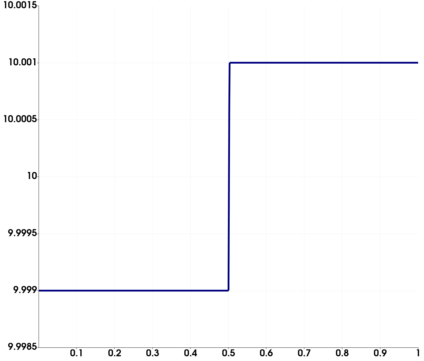
(a) $t=0$

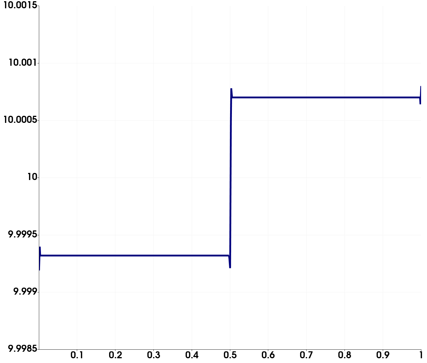
(b) $t=1/8\,t_{\text{P}}$

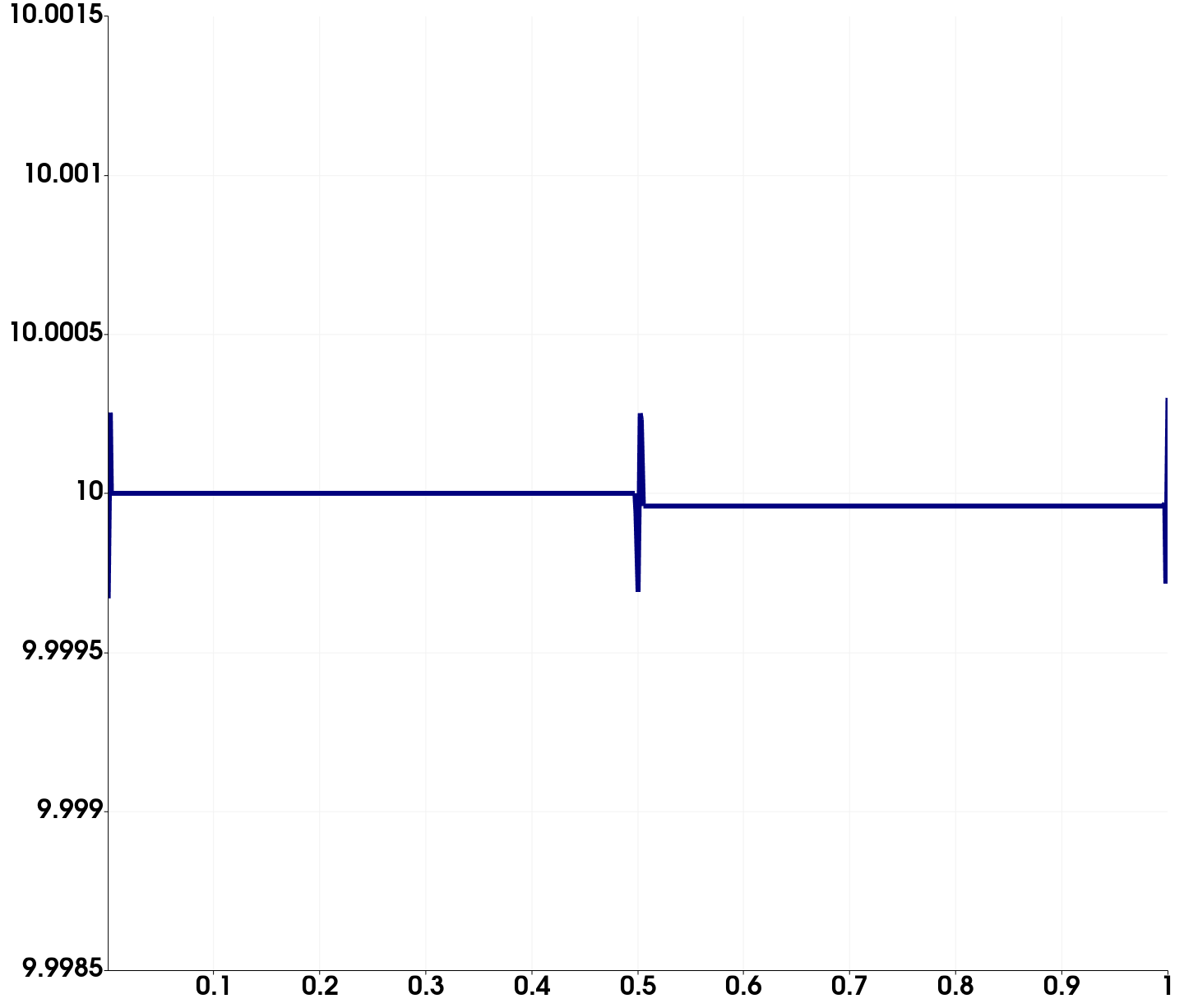
(c) $t=2/8\,t_{\text{P}}$

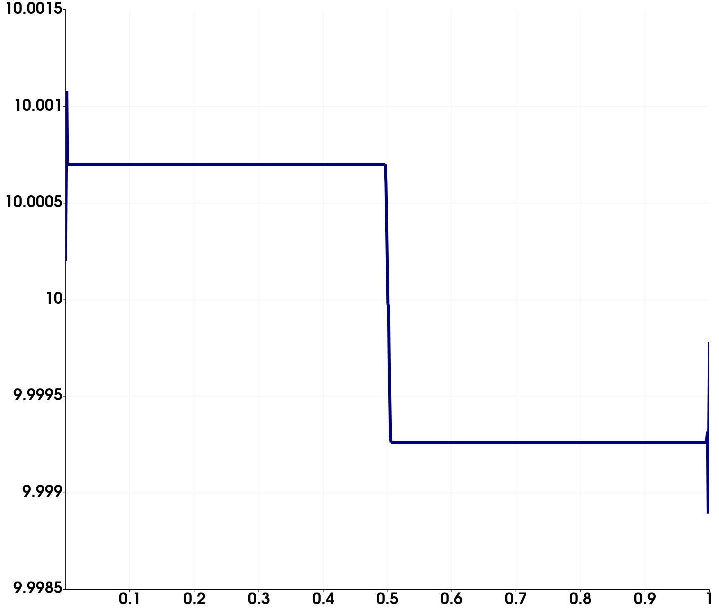
(d) $t=3/8\,t_{\text{P}}$

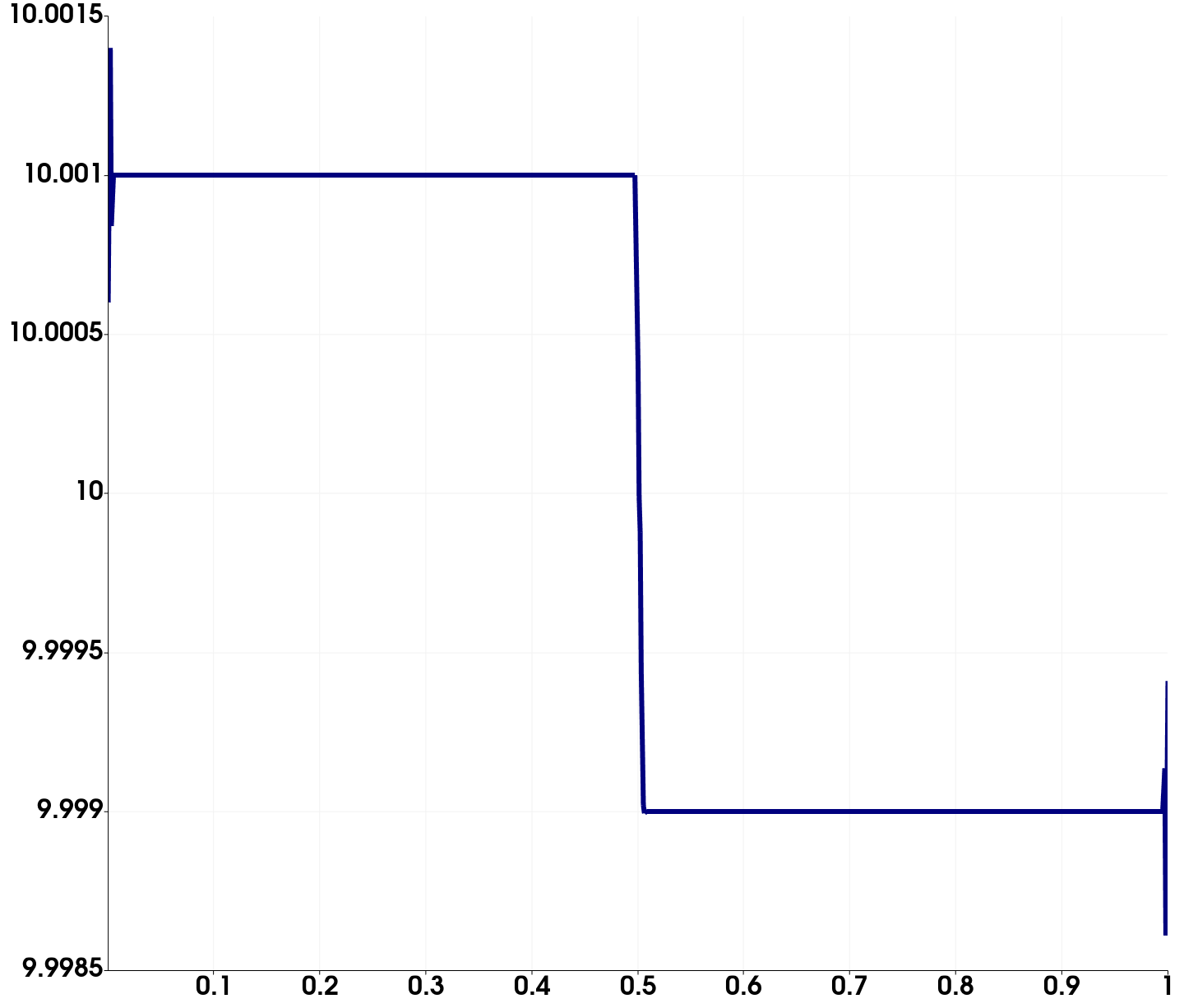
(e) $t=4/8\,t_{\text{P}}$

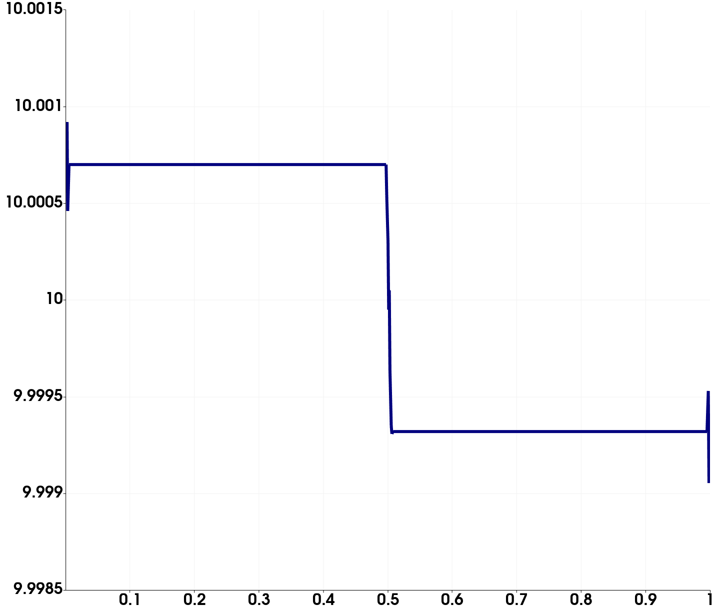
(f) $t=5/8\,t_{\text{P}}$

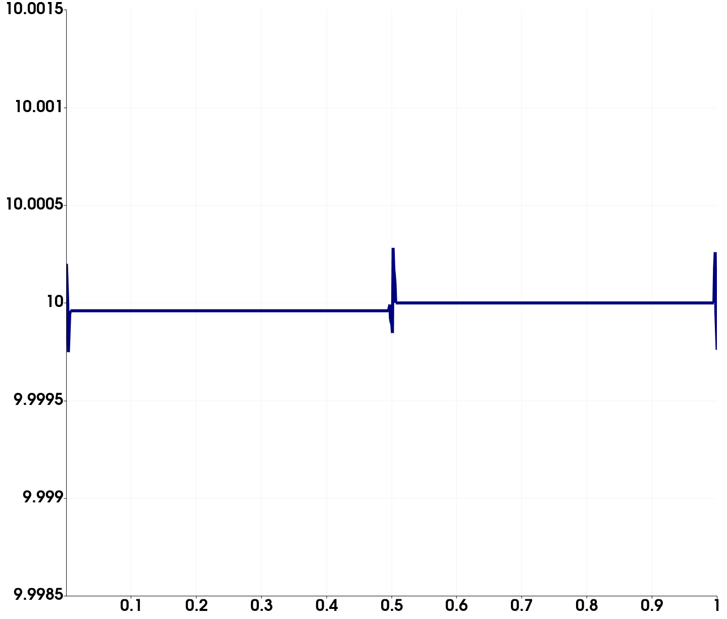
(g) $t=6/8\,t_{\text{P}}$

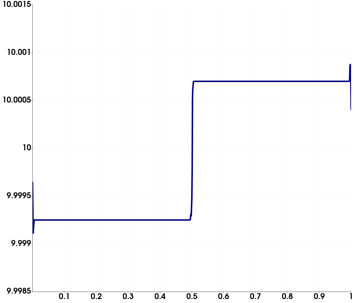
(h) $t=7/8\,t_{\text{P}}$

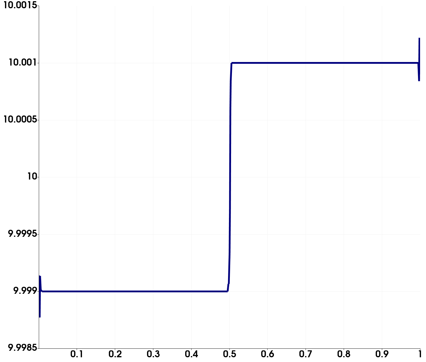
(i) $t=t_{\text{P}}$

Figure 2: Temporal snapshots of the density profile of the pure plasma oscillation test case (Definition 5.3) for a full period of plasma oscillation. The snapshots are taken approximately at times, from (a) to (i), $t=\tfrac{n-1}{8}t_{\text{P}}$, $n=1,\ldots,9$. The period of the first and final snapshot coincide. The dynamics of the system are almost purely Hamiltonian, meaning the time evolution is almost entirely dictated by (20a). The stationary contact at $x=0.5$ remains very well preserved.

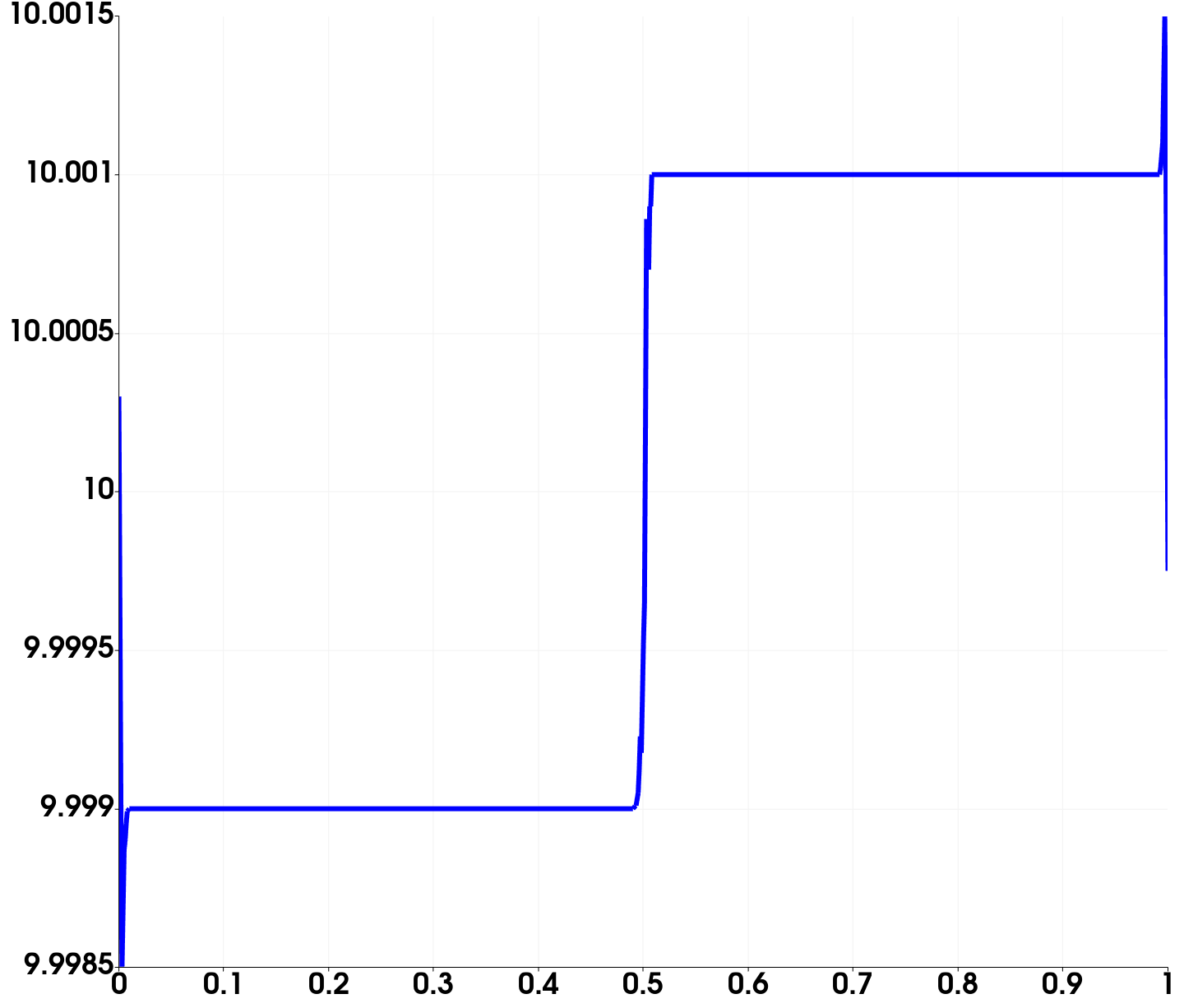
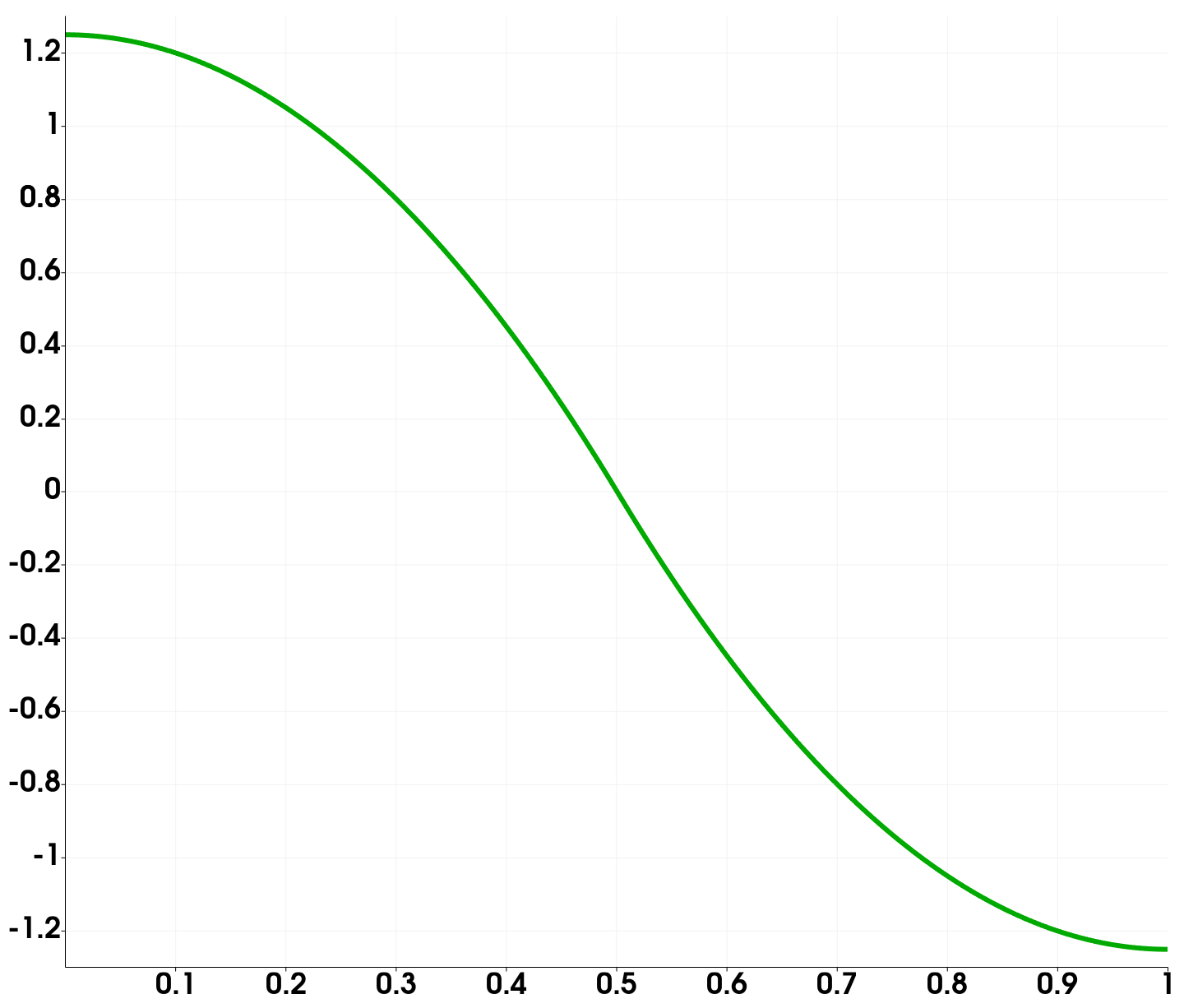
(a) no restart

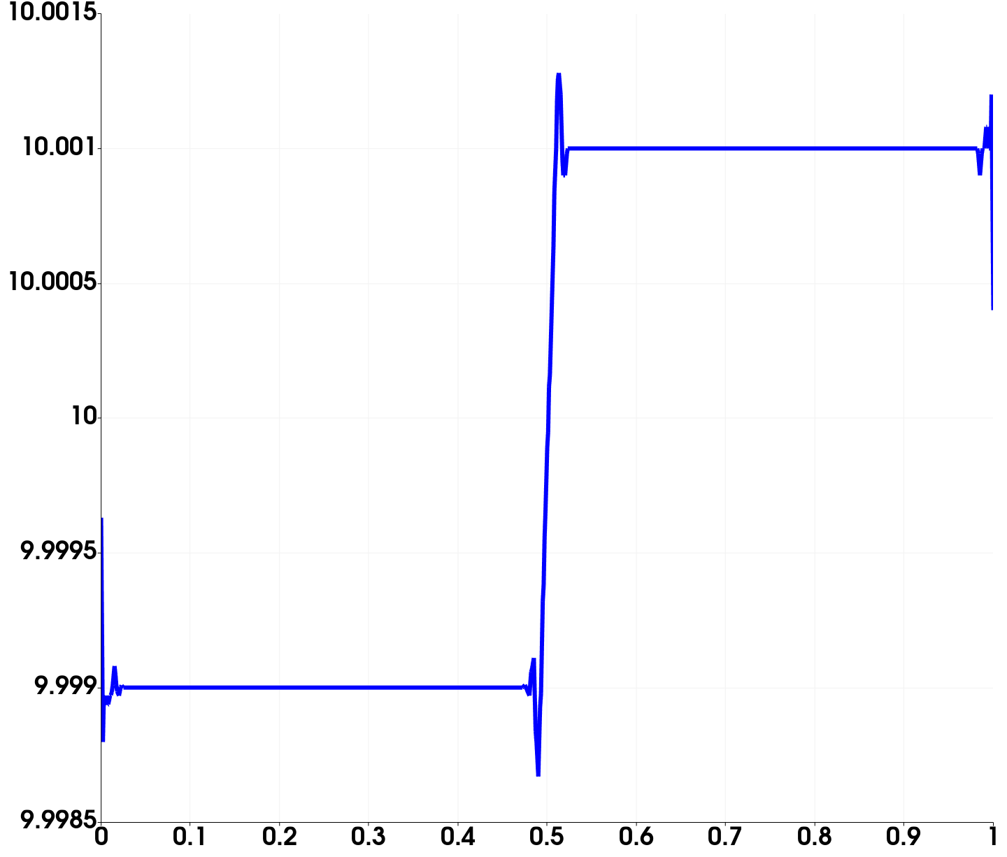
(b) relaxation

(c) full restart

Figure 3: Comparison of the effects of different choices of restart. The three top figures display the density at the final time $t_{\text{F}}=5t_{\text{P}}$, the three figures on the bottom show the potential at the final time. From left to right we use: (a) no restart, (b) relaxation, and (c) full restart. The difference between the full restart and relaxation restart is again minimal.

We now consider a numerical test case for capturing pure plasma oscillations. The initial setup is given in Definition 5.3, and consists of a quasi one-dimensional plasma with discontinuous density, no velocity, low pressure, and a positive background charge density that neutralizes the mean value of the electron charge in the domain. The purpose of prescribing a low pressure is to ensure that pressure forces $-\nabla p$ are negligible in comparison to the electric force $-\rho\nabla\varphi$.

Definition 5.3 (Plasma column).

Given the following rectangular domain and repulsive coupling constant $\alpha$,

$$\Omega=[0,1]\times[0,h]\ \ \text{with}\ \ h=400^{-1},\qquad\alpha=10^{4}\,>\,0,$$

we introduce an initial state $u_{0}(\boldsymbol{x})$ defined by the primitive quantities (density, velocity, pressure),

(50) $$\rho_{0}=\begin{cases}\overline{\rho}-\delta&\text{if }x<0.5,\\ \overline{\rho}+\delta&\text{if }x\geq 0.5,\end{cases}\quad\text{with }\overline{\rho}=10.0\text{ and }\delta=0.001,\;\mathbf{v}_{0}=\boldsymbol{0},\;p_{0}=0.01.$$

We further introduce a constant background charge density (see Section 3.6) with numerical value $\rho_{b}=-\overline{\rho}$.

With this setup the approximate value of the plasma frequency $\omega_{p}=\sqrt{\rho\,\alpha}\approx\sqrt{\overline{\rho}\alpha}=\sqrt{10^{5}}$; therefore the plasma period is $t_{\text{P}}\approx 0.01986$. We consider a final simulation time of $t_{\text{F}}=5\,t_{\text{P}}$ and enforce slip boundary conditions on the momentum, viz., $\mathbf{m}\cdot\boldsymbol{\mathrm{n}}=0$ at the boundary $\partial\Omega$, as well as homogenenous Neumann boundary conditions on the potential, $\nabla\varphi\cdot\boldsymbol{\mathrm{n}}=0$ at the boundary $\partial\Omega$. Slip boundary conditions ensure that the total mass, $\int_{\Omega}\rho(\boldsymbol{x},t)\,\mathrm{d}\boldsymbol{x}$ of the system is conserved. This ensures that the total charge density remains compatible with the Neumann boundary conditions,

$$0\;=\;\int_{\partial\Omega}\nabla\varphi\cdot\boldsymbol{\mathrm{n}}\,\mathrm{d}\boldsymbol{s}\;=\;\int_{\Omega}\Delta\varphi\,\mathrm{d}\boldsymbol{x}\;=\;\int_{\Omega}-\alpha\big{(}\rho(\boldsymbol{x},t)+\rho_{b}\big{)}\,\mathrm{d}\boldsymbol{x}\;=\;0.$$

We briefly comment on an implementational detail.

Remark 5.4 (Rank deficiency due to Neumann boundary conditions).

The stiffness matrices of the discrete Poisson problem (44) and the source update (20a) (either with bilinear form (21), or (26)) are rank deficient due to our choice of homogeneous Neumann boundary conditions for the potential. The kernel of the stiffness matrices is one dimensional and contains all constant functions in $\mathbb{H}_{h}$. In order to deal with this defect we use a mean value filter $\mathcal{P}$ to eliminate all constant modes; a detailed discussion of such filtering techniques can be found in [11]. More precisely, for a given vector $\Phi=\{\Phi_{i}\}_{i\in\mathcal{V}_{P}}$ we set

$$(\mathcal{P}\Phi)_{i} =\Phi_{i}-\mu(\Phi),\quad\text{for }i\in\mathcal{V}_{P},\text{ where}\quad\mu(\Phi)=\frac{1}{|\Omega|}\sum_{j\in\mathcal{V}_{P}}m_{j}\Phi_{j}.$$

The mean value filter is now applied to all right hand sides to ensure that the right hand side vector is in the column space of the stiffness matrix. Moreover, the mean value filter should also be applied to intermediate updates after every multiplication with the stiffness matrix when solving with a Krylov space method, such as conjugate gradient method.

We note that our choice of source update scheme does not require a CFL condition; see Sections 3.3 and 3.4. This implies that the full algorithm is only subject to a hyperbolic CFL condition; see Apppendix A. In fact, using a (relative) CFL number of $0.75$ we encounter only a very mild hyperbolic CFL constraint resulting in time step sizes of about $\tau\,\sim\,1.25\,t_{\text{P}}$. While this is an ideal situation—resolving the plasma frequency is not required—we nevertheless want to fully resolve plasma oscillations in this case. We thus choose a very small relative CFL number of $0.005$.

Figure 2 shows nine temporal snapshots of the density of a simulation covering a full plasma period (out of the total of five periods simulated). We used the source update scheme (20a) with bilinear form (26), and strategy (a), no restart of the Gauß law. Most noticeably the stationary contact at $x=0.5$ is very well preserved.

Figure 3 shows a comparison of the effect of our three different choices of restart, (a) no restart, (b) relaxation, and (c) full restart. We note that the difference between the full restart and relaxation restart are minimal. A slightly more pronounced Gibbs phenomenon at the stationary contact is visible for both restart strategies in comparison to strategy (a), no restart.

5.3 Electrostatic Implosion

We now consider an electrostatic implosion configuration in a circular domain $\Omega$ of radius $r_{3}=16$, that is, $\Omega=\{\boldsymbol{x}\in\mathbb{R}^{2}\;:\;|\boldsymbol{x}|_{\ell^{2}}\leq r_{3}\}$, with boundary conditions $\mathbf{p}\cdot\boldsymbol{\mathrm{n}}=0$ and $\varphi=0$ on the entirety of $\partial\Omega$ and the parameters $\alpha=10^{3}$, and $\gamma=5/3$. The initial state is uniform with density $\rho_{0}=1$, velocity $\mathbf{v}_{0}=\boldsymbol{0}$, and pressure $p_{0}=10^{-4}$. Given radii $r_{2}=6$ and $r_{1}=4$ we consider a constant background charge density $\rho_{b}$ defined as follow:

(51) $$\rho_{b}(\boldsymbol{x})\;=\;\begin{cases}10000&\text{if }r_{1}<|\boldsymbol{x}|_{\ell^{2}}\leq r_{2},\\ 0&\text{otherwise}.\end{cases}$$

The final time is set to $t_{\text{F}}=\tfrac{3}{64}t_{\text{P}}$, where $t_{\text{P}}=\tfrac{2\pi}{\omega_{p}}$, and $\omega_{p}=\sqrt{\rho_{0}\alpha}=\sqrt{10^{3}}$.

This geometric setup is similar to considering a configuration with two concentric cylindrical electrodes, with the outer electrode grounded and the inner electrode having a very high positive voltage pulling the electron gas inwards. As the bulk of the electron fluid is accelerated towards the center a cylindrical outer region with very low density and low pressure is left behind. Such a configuration with strong implosion and compression and an emerging near-vacuum region are well-known to be hydrodynamically highly unstable, see for instance [60, 27]. The configuration is an excellent starting point to judge the merits of the scheme in relationship to its ability to work in the shock hydrodynamics regime (discontinuous solutions and strong expansions). The configuration leads to large material velocities which necessitates small time-step sizes due to the hyperbolic CFL condition (53). On the other hand the plasma frequency is moderate. This implies that the smallest time-scale (that has to be resolved) is dominated by the hydrodynamic subsystem and not by electrostatic effects. A reference computation with 1M quadrilaterals visualizing the dynamics is shown in Figure 5. Temporal snapshots of three different computations with different choices of restart (no restart, relaxation, full restart) are given in Figure 5. All in all, the qualitative difference of all three computations is minimal. All of them seem to capture the dynamics accurately and are close to the reference computation 5 (h).

(a) $t=1/16\,t_{\text{F}}$

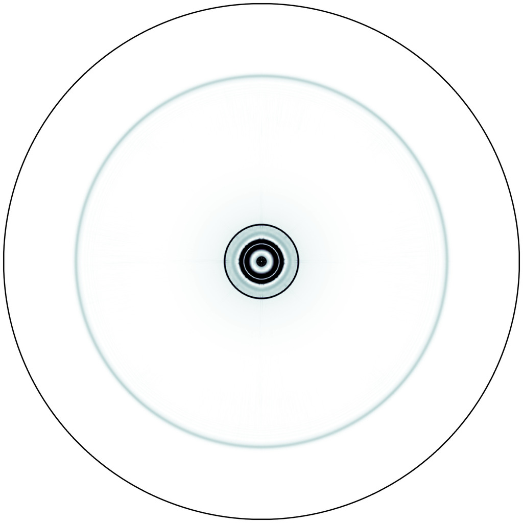
(b) $t=1/8\,t_{\text{F}}$

(c) $t=2/8\,t_{\text{F}}$

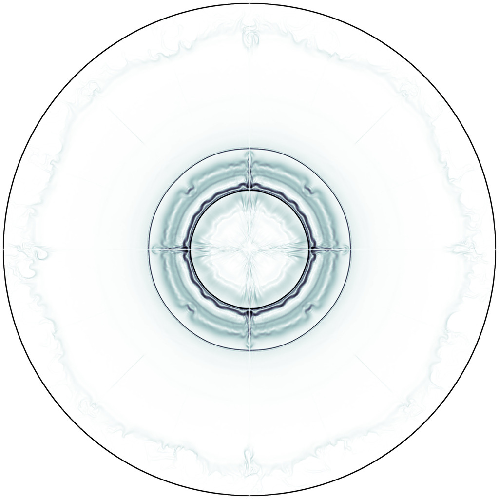
(d) $t=3/8\,t_{\text{F}}$

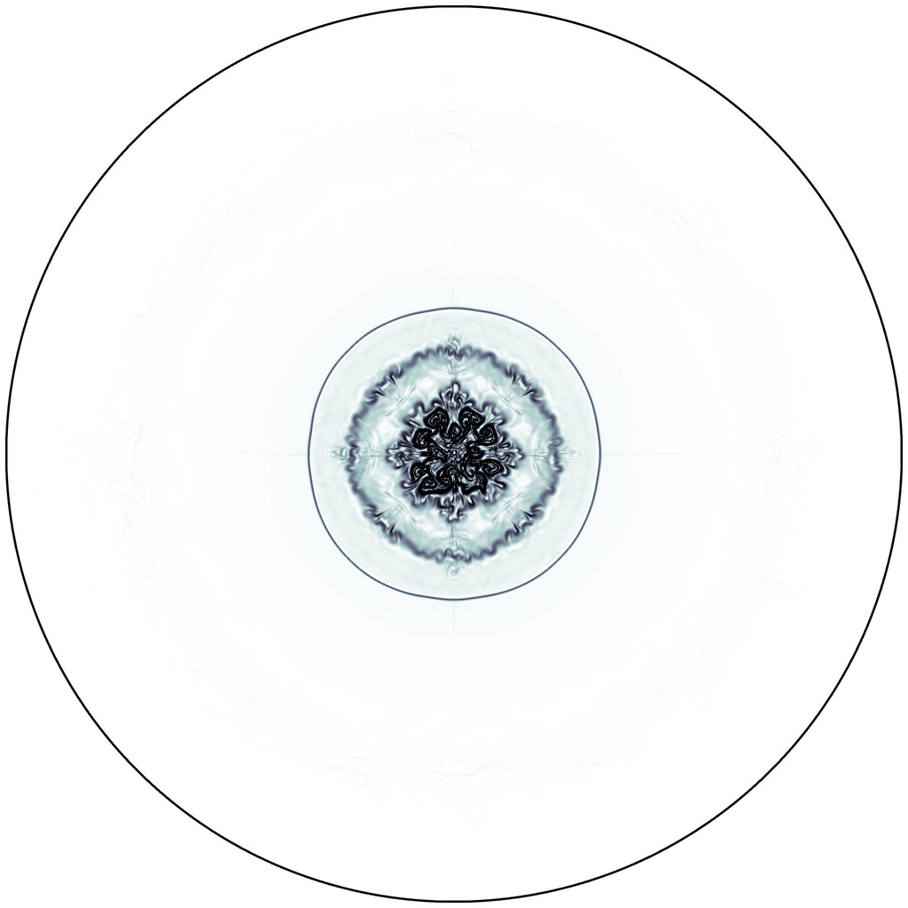
(e) $t=4/8\,t_{\text{F}}$

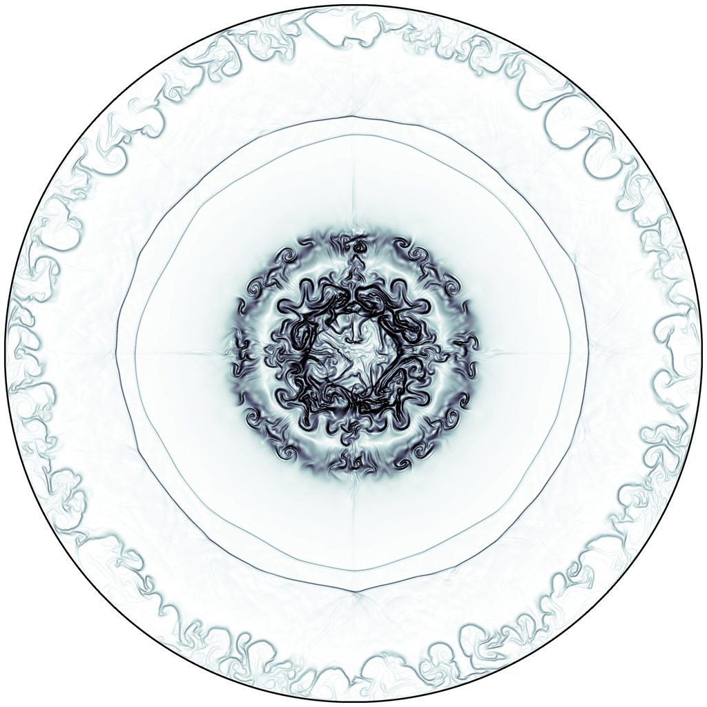
(f) $t=5/8\,t_{\text{F}}$

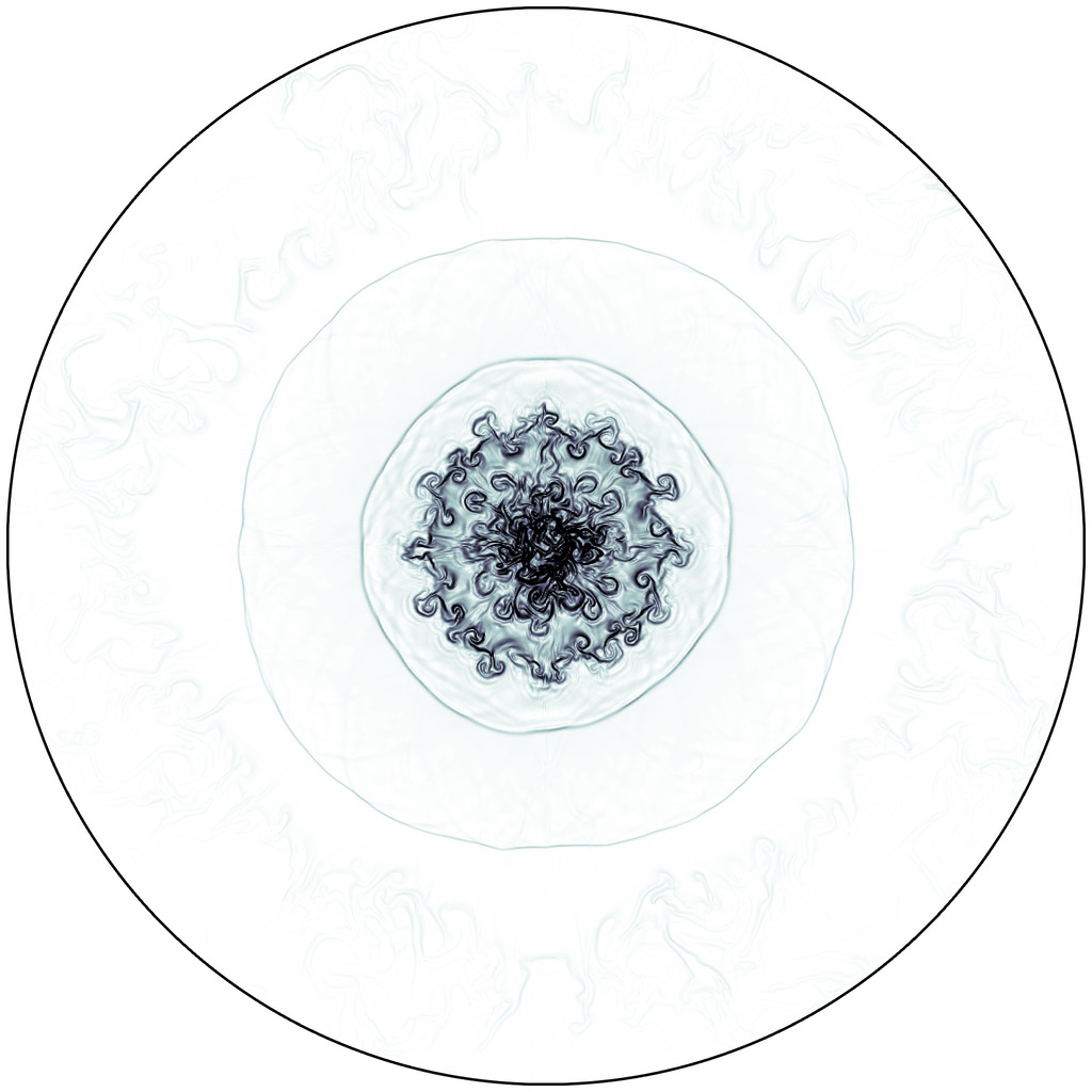
(g) $t=6/8\,t_{\text{F}}$

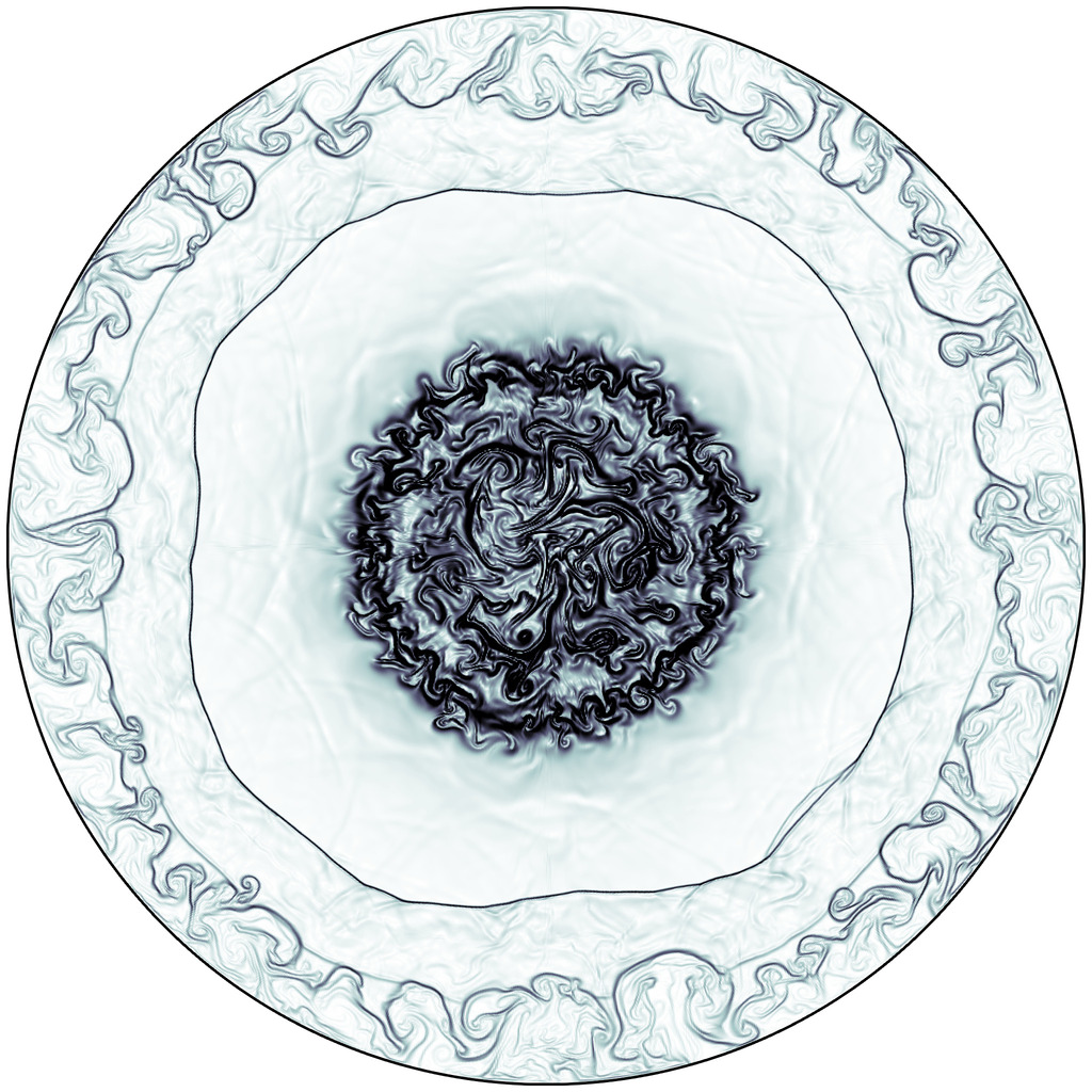
(h) $t=7/8\,t_{\text{F}}$

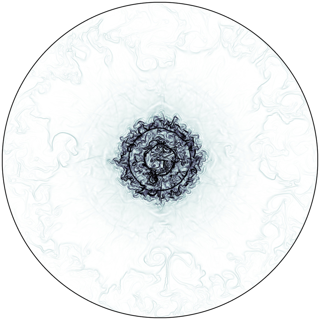
(i) $t=F_{f}$

Figure 4: Temporal snapshots of a schlieren plot of the density profile of the electrostatic implosion test case. Reference computation with full restart and approximately 1M quadrilaterals.

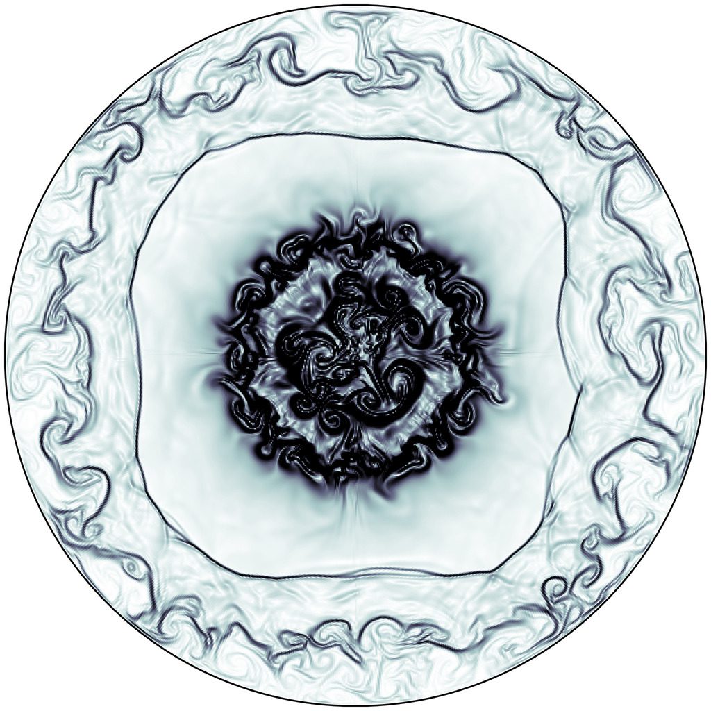
(a) no restart

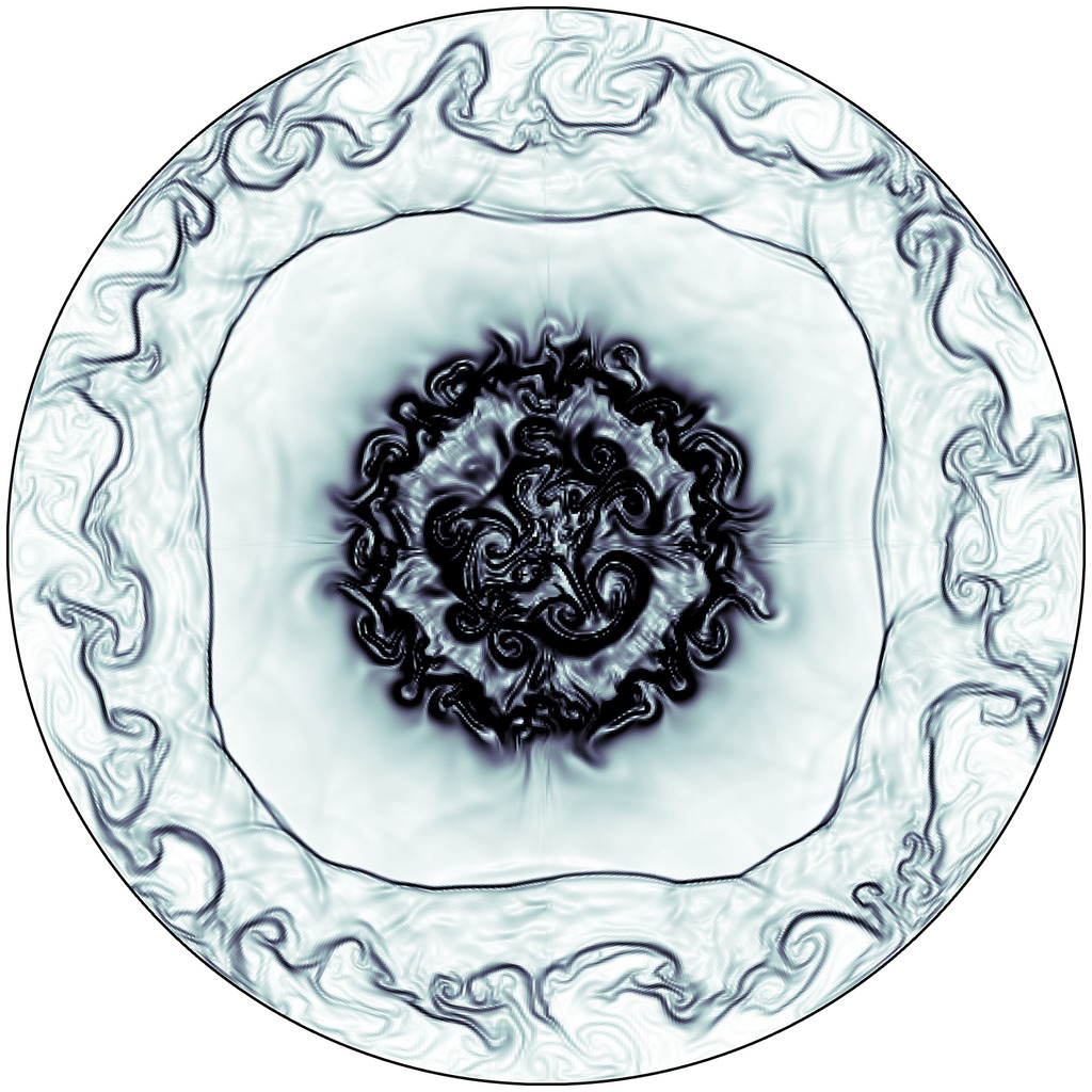
(b) relaxation

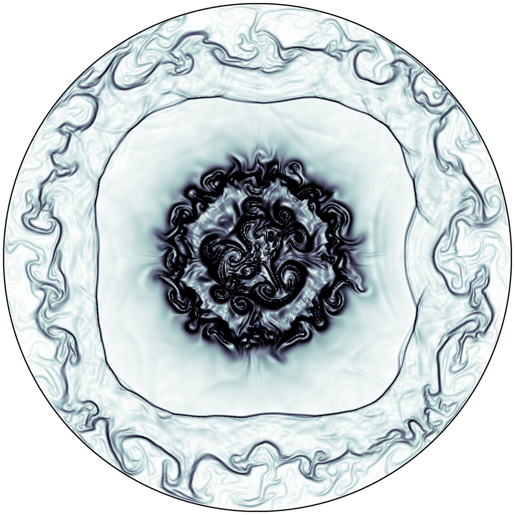
(c) full restart

Figure 5: Comparison of the effects of different choices of restart on the electrostatic implosion test case. The snapshots are taken at $t=\tfrac{7}{8}t_{\text{F}}$ and show a schlieren plot of the density profile. From left to right we use: (a) no restart, (b) relaxation, and (c) full restart.

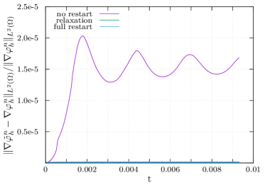
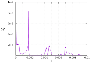
Figure 6: Norm of the Gauß law residual (45) as a function of time for three different choices of restart, (a) no restart, (b) relaxation, and (c) full restart. The curves for relaxation restart and full restart lie on top of each other.

Figure 7: Relaxation parameter $\lambda_{P}^{n}$ as a function of time for the relaxation strategy. The scale had been clipped at 1.0e-2. The maximum $\lambda_{P}^{N}$ occurs during the first step and has a magnitude of around 2.0e-1.

As an additional figure of merit we report the Gauß-law residual (45) as a function of time for all three choices of restart in Figure 7. We highlight that the Gauß-law residual for the no-restart strategy accumulates a maximal relative deviation of around 2e-5 after about about 47,000 time-steps. Bearing in mind that this is a complex simulation with a non-smooth solution this is an excellent result. The residual for the other two choices of restart remains in the 1e-8 range and are not distinguishable in Figure 7.

An important aspect of the relaxation technique is the prospect that it can maintain the (discrete) Gauß-law exactly with only a minimal correction to the kinetic energy. Figure 7 indeed corroborates this observation: The numerical value of the relaxation parameter $\lambda^{n}_{P}$ is almost always well below 2e-3 throughout the computation.

6 Conclusion and outlook

In this paper we have discussed a fully discrete numerical scheme for the Euler-Poisson system that preserves the invariant domain of the Euler subsystem, as well as energy stability properties. We have demonstrated that the Gauss law can also be preserved at the same time with a simple postprocessing technique that introduces a mild amount of artificial relaxation to the system.

In order to satisfy energy stability as well as well-posedness of the linear algebra system associated to each time step, the source update scheme requires special attention in regards to the choice of finite element spaces and quadrature rules. In particular, we have made extensive use of lumped quadratures. This presents no obstacle for the case of simplicial affinely mapped elements. However, it is a delicate issue in the context of quadrilateral/hexahedral meshes, where it is well known that element distortion can degrade second-order accuracy. We have shown that our proposed scheme exhibits second-order accuracy in the context of asymptotically affine mesh sequences (of quadrilaterals) which are the family of nested meshes most frequently used in practice.

In a sequence of numerical experiments we have verified and highlighted qualitative and quantitative properties of the scheme. In addition to the grid convergence results used to understand the effects of mesh distortion, we have also demonstrated robustness of our scheme when simulating pure plasma oscillation with minimal gas effects, as well as an electrostatic implosion test highlighting our capabilities in the shock-hydrodynamics regime.

The results presented in this paper are first building block in a larger effort of targeting the development of numerical methods for the full Euler-Maxwell system. A future publication will discuss the application of our scheme to systems incorporating magnetic field effects. A crucial property for us to demonstrate in this context will be the ability to overstep the plasma or cyclotron frequency similarly as we discussed in the present manuscript.

Appendix A Graph-based hyperbolic solver

For the hyperbolic subsystem we use a framework of numerical schemes based on a graph-viscosity stabilization and convex limiting [39, 40, 37, 42, 49]. The framework is discretization agnostic, meaning that it can in principle be used in conjunction with continuous or discontinuous finite element, finite volume, or finite difference formulations. In this paper, however, we use a discontinuous finite element ansatz for reasons discussed in Section 3 regarding energy stability. For the sake of completeness and reproducibility we summarize some implementational aspects in this appendix, for a complete overview of the methodology we refer the reader to [42]. Numerical methods, that can preserve convex constraints of the solution (e.g. positivity properties), are also advanced in [68, 69, 71] and references therein.

A.1 Discrete divergence operator and stencil

For every element $K\in\mathcal{T}_{h}$, we define the following set of indices

$$\mathcal{I}(K) :=\big{\{}i\in\mathcal{V}\ |\ \phi_{i|K}\not\equiv 0\big{\}}\,,$$

That is, $\mathcal{I}(K)$ is the set of all shape functions with support on the interior of the element $K$. For every $i\in\mathcal{I}(K)$ and every $j\in\mathcal{V}$ we define the vector $\mathbf{c}_{ij}\in\mathbb{R}^{d}$ as

$$\mathbf{c}_{ij}:=\begin{cases}\mathbf{c}_{ij}^{K}-\mathbf{c}_{ij}^{\partial K}\;&\text{if }j\in\mathcal{I}(K),\\ \mathbf{c}_{ij}^{\partial K}&\text{if }j\in\mathcal{V}\backslash\mathcal{I}(K),\end{cases}$$

where

$$\mathbf{c}_{ij}^{K}:=\int_{K}\phi_{i}\nabla\phi_{j}\,\mathrm{d}\boldsymbol{x},\qquad\mathbf{c}_{ij}^{\partial K}:=\frac{1}{2}\int_{\partial K\backslash\partial\Omega}\phi_{j}\phi_{i}\boldsymbol{\mathrm{n}}_{K}\,\mathrm{d}\boldsymbol{s}.$$

where $\boldsymbol{\mathrm{n}}_{K}$ is the outwards pointing normal of the element $K$. Note that: $\mathbf{c}_{ij}^{\partial K}$ is necessarily zero if $\phi_{j}$ does not have support on the element $K$ or on one of its immediate neighbors. With this observation in mind, we define the stencil at the node $i$ as follows:

$$\mathcal{I}(i)=\{j\in\mathcal{V}\;|\;\mathbf{c}_{ij}\not=0\}.$$

The set of vectors $\{\mathbf{c}_{ij}\}_{j\in\mathcal{I}(i)}$ is used to construct an approximation of the divergence operator at each node $i$ in the spirit of a collocation scheme [42]. We highlight that this approximation of the divergence operator is consistent with the polynomial degree of the shape functions $\{\phi_{i}\}_{i\in\mathcal{V}}$ and works with arbitrary meshes, see [42] for more details.

A.2 Scheme

For a given state $\mathbf{U}_{i}^{n}$ we define a low-order update $\mathbf{U}_{i}^{n+1,\mathrm{L}}$ approximating the solution of (5) as follows:

(52) $$m_{i}\frac{\mathbf{U}_{i}^{n+1,\mathrm{L}}-\mathbf{U}_{i}^{n}}{\tau}+\sum_{j\in\mathcal{I}(i)}\mathbb{f}(\mathbf{U}_{j}^{n})\,\mathbf{c}_{ij}-d_{ij}^{n,\mathrm{L}}(\mathbf{U}_{j}^{n}-\mathbf{U}_{i}^{n})=0,\text{for all }i\in\mathcal{V},$$

where we have set $m_{i}=\int_{\Omega}\phi_{i}\,\mathrm{d}\boldsymbol{x}$, and where $\mathbb{f}(\mathbf{U}_{j}^{n})\in\mathbb{R}^{(d+2)\times d}$ is the flux at the node $j\in\mathcal{I}(i)$, and $d_{ij}^{n,\mathrm{L}}\in\mathbb{R}^{+}$ is a viscosity coefficient defined as

$$d_{ij}^{n,\mathrm{L}}:=\max\{\lambda^{\text{max}}(\mathbf{U}_{i}^{n},\mathbf{U}_{j}^{n},\mathbf{n}_{ij})|\mathbf{c}_{ij}|_{\ell^{2}},\lambda^{\text{max}}(\mathbf{U}_{j}^{n},\mathbf{U}_{i}^{n},\mathbf{n}_{ji})|\mathbf{c}_{ji}|_{\ell^{2}}\}$$

Here, $\lambda^{\text{max}}(\mathbf{U}_{L},\mathbf{V}_{R},\mathbf{n})$ is any upper-bound on the maximum wavespeed of propagation of the projected-Riemann problem (setting $x:=\boldsymbol{x}\cdot\boldsymbol{\mathrm{n}}$):

$$\partial_{t}\mathbf{U}+\partial_{x}(\boldsymbol{\mathbb{f}}(\mathbf{U})\cdot\boldsymbol{\mathrm{n}})=0\quad\text{with initial data}\quad\mathbf{U}_{0}=\begin{cases}\mathbf{U}_{L}&\text{if }x\leq 0,\\ \mathbf{U}_{R}&\text{if }x>0,\\ \end{cases}$$

and we set $d_{ii}^{n,\mathrm{L}}=-\sum_{j\in\mathcal{I}{(i)}\backslash\{i\}}d_{ij}^{n,\mathrm{L}}$. Then under the hyperbolic CFL condition

(53) $$\tau_{n}:=-\text{c}_{\text{cfl}}\min_{i\in\mathcal{V}}\tfrac{m_{i}}{2d_{ii}^{n,\mathrm{L}}}$$

the update $\mathbf{U}_{i}^{n+1,\mathrm{L}}$ as defined by (52) maintains the invariant domain $\mathcal{A}$ [39, 40, 37, 42], viz.,

(54) $$\mathbf{U}_{i}^{n+1,\mathrm{L}}\;\in\;\mathcal{A}\;:=\;\big{\{}\mathbf{u}=(\rho,\mathbf{m},\mathcal{E})\text{ such that }\rho>0,\ e>0,\ s(e,\rho)\geq s_{\min}\big{\}}.$$

High-order update and convex limiting

We also introduce a corresponding high-order method,

$$m_{i}\frac{\mathbf{U}_{i}^{n+1,\mathrm{H}}-\mathbf{U}_{i}^{n}}{\tau_{n}}+\sum_{j\in\mathcal{I}(i)}\mathbb{f}(\mathbf{U}_{j}^{n})\,\mathbf{c}_{ij}-d_{ij}^{n,\mathrm{H}}(\mathbf{U}_{j}^{n}-\mathbf{U}_{i}^{n})=0,$$

where the only difference with the low-order scheme (52) lies in the choice of a high-order viscosity $d_{ij}^{n,\mathrm{H}}$. The high-order graph viscosities are typically constructed such that $d_{ij}^{n,\mathrm{H}}\approx d_{ij}^{n,\mathrm{L}}$ near shocks and discontinuities, but $d_{ij}^{n,\mathrm{H}}\approx 0$ in smooth regions of the solution. A possible choice is to construct local indicators estimating the entropy production or local smoothness of the solution and use those to construct the high-order viscosity [41, 37]. In the computations reported in this manuscript, however, we use a very simple approach by setting

$$d_{ij}^{n,\mathrm{H}}=\begin{cases}d_{ij}^{n,\mathrm{L}}&\text{if }\boldsymbol{x}_{i}=\boldsymbol{x}_{j},\\ 0&\text{otherwise}.\end{cases}$$

This definition is equivalent to using the low-order viscosity only on the faces of the elements. We observe numerically good convergence rates for $\mathbb{P}^{1}$ and $\mathbb{Q}^{1}$ elements.

The high-order solution $\mathbf{U}_{i}^{n+1,\mathrm{H}}$ it is not invariant domain preserving and can consequently not be used directly [37]. In order to maintain invariant domain preservation and the high approximation order we blend the low-order solution and high-order solution together in a postprocessing step by setting

$$\mathbf{U}_{i}^{n+1}=\mathbf{U}_{i}^{n+1,\mathrm{L}}+\sum_{j\in\mathcal{I}(i)}\ell_{ij}\mathbf{A}_{ij}\quad\text{with}\quad\mathbf{A}_{ij}:=\tau_{n}(d_{ij}^{n,\mathrm{H}}-d_{ij}^{n,\mathrm{L}})(\mathbf{U}_{j}^{n}-\mathbf{U}_{i}^{n}).$$

Here, the limiter matrix $\ell_{ij}\in[0,1]$ is computed with a convex limiter consisting of directional line searches that ensures that $\mathbf{U}_{i}^{n+1}\in\mathcal{A}$ [37, 42].

Remark A.1 (Time-step size constraint).

We note that the time-step constraint (53) depends on the low order viscosities $\{d_{ij}^{n,\mathrm{L}}\}_{j\in\mathcal{I}(i)\backslash\{i\}}$. The time-step size constraint (53) is sufficient for the first-order scheme, but it is overly pessimistic when applied to a high-order method. It is possible to use sharper time-step size constraint estimates for high order methods/viscosities. However, for the sake of simplicity, and in order to avoid digression, in this manuscript we use (53), computed with the low-order viscosities, even when we are actually using a high order method.

A.3 High-order time stepping

The scheme introduced so far is high order in space and first order in time. In order to recover higher order convergence in time the basic forward Euler step is now used as a basic building block in a high-order SSP Runge-Kutta method [58]. For implementational details we refer the reader to [36, 35, 49].

Appendix B Partial restart of the potential with line search

An alternative approach to the artificial relaxation discussed in Section 4.2 is to perform a line search blending $\varphi_{h}^{n+1}$ computed with the update procedure (Algorithm 4, or 5 respectively) and $\tilde{\varphi}_{h}^{n+1}$ computed by solving (44) such that the final update is as close to the restarted potential $\tilde{\varphi}_{h}^{n+1}$ as possible while maintaining the energy inequality. To this end we introduce a linear combination

(55) $$\varphi^{n+1,\lambda}_{h}\in\mathbb{H}_{h},\qquad\Phi_{i}^{n+1,\lambda}\;=\;(1-\lambda_{i})\Phi_{i}^{n+1}\;+\;\lambda_{i}\tilde{\Phi}_{i}^{n+1},$$

where $\lambda_{i}\in[0,1]$, $i\in\mathcal{V}_{P}$, is determined by an optimization problem,

(56) $$\min_{\lambda\in[0,1]}\;\|\varphi_{h}^{n+1,\lambda}-\tilde{\varphi}_{h}^{n+1}\|_{\mathbf{L^{2}(\Omega)}}^{2}\;\text{subject to}\;\big{\|}\nabla\varphi_{h}^{n+1,\lambda}\big{\|}_{\mathbf{L}^{2}(\Omega)}^{2}\leq\big{\|}\nabla\varphi_{h}^{n+1}\big{\|}_{\mathbf{L}^{2}(\Omega)}^{2}.$$

This ensures that setting $\varphi_{h}^{n+1}\leftarrow\varphi_{h}^{n+1,\lambda}$ maintains the total energy balance (37) while closing the difference between $\varphi_{h}^{n+1,\lambda}$ and the discrete Gauß law abiding $\tilde{\varphi}_{h}^{n+1}$ as much as possible. In light of the heuristic error estimate established in Lemma 4.1 the hope arises that $\lambda_{i}$ can generally be chosen very close to $1$.

The proposed optimization problem can be modified in a number of ways. For example, the computational cost of the optimization problem can be reduced significantly by introducing a convenient lumping and allow for possible overrelaxation. Suppose the inequality constraint in (56) is active. The Lagrange conditions then read

$$\sum_{j\in\mathcal{I}(i)}\big{(}\tilde{\Phi}_{i}^{n+1}-\Phi_{i}^{n+1}\big{)}\,\big{(}m_{ij}+\mu\mathcal{K}_{ij}\big{)}\,\big{(}\tilde{\Phi}_{j}^{n+1}-\Phi_{j}^{n+1}\big{)}\,(1-\lambda_{j})\;=\;\\ \sum_{j\in\mathcal{I}(i)}\big{(}\tilde{\Phi}_{i}^{n+1}-\Phi_{i}^{n+1}\big{)}\,\big{(}\mu\mathcal{K}_{ij}\big{)}\,\tilde{\Phi}_{j}^{n+1},$$

where $\mathcal{K}$ is the stiffness matrix as introduced in Section 3.1 and $\mu$ is a Lagrange multiplier. Lumping the matrices on the left-hand side then leads to an algebraic condition of the form:

$$\big{(}\tilde{\Phi}_{i}^{n+1}-\Phi_{i}^{n+1}\big{)}^{2}\,m_{i}\,(1-\lambda_{i})\;=\;\\ \sum_{j\in\mathcal{I}(i)}\big{(}\tilde{\Phi}_{i}^{n+1}-\Phi_{i}^{n+1}\big{)}\,\big{(}\mu\mathcal{K}_{ij}\big{)}\,\tilde{\Phi}_{j}^{n+1},$$

This can be efficiently solved by setting

$$\tilde{\lambda}_{i}\;:=\;\frac{\sum_{j\in\mathcal{I}{(i)}}\mathcal{K}_{ij}\tilde{\Phi}_{j}^{n+1}}{m_{i}\,\big{(}\tilde{\Phi}_{i}^{n+1}-\Phi_{i}^{n+1}\big{)}},\quad\mu\;=\;\frac{\sum_{i,j}2\,\mathcal{K}_{ij}\tilde{\Phi}_{i}^{n+1}\,\tilde{\lambda}_{j}\big{\{}\Phi_{j}^{n+1}-\tilde{\Phi}_{j}^{n+1}\big{\}}}{\sum_{i,j}\mathcal{K}_{ij}\tilde{\lambda}_{i}\big{\{}\Phi_{i}^{n+1}-\tilde{\Phi}_{i}^{n+1}\big{\}}\tilde{\lambda}_{j}\big{\{}\Phi_{j}^{n+1}-\tilde{\Phi}_{j}^{n+1}\big{\}}}.$$

References

- [1] A. S. Almgren, V. E. Beckner, J. B. Bell, M. Day, L. H. Howell, C. Joggerst, M. Lijewski, A. Nonaka, M. Singer, and M. Zingale, Castro: A new compressible astrophysical solver. i. hydrodynamics and self-gravity, The Astrophysical Journal, 715 (2010), p. 1221.
- [2] M. Alnæs, J. Blechta, J. Hake, A. Johansson, B. Kehlet, A. Logg, C. Richardson, J. Ring, M. E. Rognes, and G. N. Wells, The fenics project version 1.5, Archive of Numerical Software, 3 (2015).
- [3] R. Anderson, J. Andrej, A. Barker, and et al., MFEM: A modular finite element methods library, Comput. Math. Appl., 81 (2021), pp. 42–74.
- [4] D. Arndt, W. Bangerth, B. Blais, M. Fehling, R. Gassmöller, T. Heister, L. Heltai, U. Köcher, M. Kronbichler, M. Maier, P. Munch, J.-P. Pelteret, S. Proell, K. Simon, B. Turcksin, D. Wells, and J. Zhang, The deal.II Library, Version 9.3, Journal of Numerical Mathematics, 29 (2021), pp. 171–186.
- [5] D. Arndt, W. Bangerth, D. Davydov, T. Heister, L. Heltai, M. Kronbichler, M. Maier, J.-P. Pelteret, B. Turcksin, and D. Wells, The deal.II finite element library: design, features, and insights, Computers & Mathematics with Applications, 81 (2021), pp. 407–422, http://arxiv.org/abs/1910.13247.
- [6] D. N. Arnold, D. Boffi, and R. S. Falk, Approximation by quadrilateral finite elements, Math. Comp., 71 (2002), pp. 909–922.
- [7] D. N. Arnold, R. S. Falk, and R. Winther, Finite element exterior calculus, homological techniques, and applications, Acta Numer., 15 (2006), pp. 1–155.
- [8] S. Badia, J. Bonilla, S. Mabuza, and J. N. Shadid, On differentiable local bounds preserving stabilization for Euler equations, Comput. Methods Appl. Mech. Engrg., 370 (2020), pp. 113267, 22.
- [9] C. Bardos, L. Erdős, F. Golse, N. Mauser, and H.-T. Yau, Derivation of the Schrödinger-Poisson equation from the quantum -body problem, C. R. Math. Acad. Sci. Paris, 334 (2002), pp. 515–520.
- [10] J. A. Bittencourt, Fundamentals of plasma physics, Springer Science & Business Media, 2004.
- [11] P. Bochev and R. B. Lehoucq, On the finite element solution of the pure Neumann problem, SIAM Rev., 47 (2005), pp. 50–66.
- [12] P. B. Bochev and J. M. Hyman, Principles of mimetic discretizations of differential operators, in Compatible spatial discretizations, vol. 142 of IMA Vol. Math. Appl., Springer, New York, 2006, pp. 89–119.
- [13] D. Boffi, F. Brezzi, and M. Fortin, Mixed finite element methods and applications, vol. 44 of Springer Series in Computational Mathematics, Springer, Heidelberg, 2013.
- [14] L. Botti, Influence of reference-to-physical frame mappings on approximation properties of discontinuous piecewise polynomial spaces, J. Sci. Comput., 52 (2012), pp. 675–703.
- [15] G. L. Bryan, M. L. Norman, B. W. O’Shea, T. Abel, J. H. Wise, M. J. Turk, D. R. Reynolds, D. C. Collins, P. Wang, S. W. Skillman, et al., Enzo: An adaptive mesh refinement code for astrophysics, The Astrophysical Journal Supplement Series, 211 (2014), p. 19.
- [16] E. Cancès, M. Defranceschi, W. Kutzelnigg, C. Le Bris, and Y. Maday, Computational quantum chemistry: a primer, in Handbook of numerical analysis, Vol. X, Handb. Numer. Anal., X, North-Holland, Amsterdam, 2003, pp. 3–270.
- [17] D. Chae and E. Tadmor, On the finite time blow-up of the Euler-Poisson equations in , Commun. Math. Sci., 6 (2008), pp. 785–789.
- [18] C. Chalons, M. Girardin, and S. Kokh, An all-regime Lagrange-projection like scheme for the gas dynamics equations on unstructured meshes, Commun. Comput. Phys., 20 (2016), pp. 188–233.
- [19] J. Chan, R. J. Hewett, and T. Warburton, Weight-adjusted discontinuous Galerkin methods: wave propagation in heterogeneous media, SIAM J. Sci. Comput., 39 (2017), pp. A2935–A2961.
- [20] P. Chandrashekar and C. Klingenberg, A second order well-balanced finite volume scheme for Euler equations with gravity, SIAM J. Sci. Comput., 37 (2015), pp. B382–B402.
- [21] P. Crispel, P. Degond, and M.-H. Vignal, An asymptotically stable discretization for the Euler-Poisson system in the quasi-neutral limit, C. R. Math. Acad. Sci. Paris, 341 (2005), pp. 323–328.
- [22] P. Crispel, P. Degond, and M.-H. Vignal, An asymptotic preserving scheme for the two-fluid Euler-Poisson model in the quasineutral limit, J. Comput. Phys., 223 (2007), pp. 208–234.
- [23] M. M. Crockatt, S. Mabuza, J. N. Shadid, S. Conde, T. M. Smith, and R. P. Pawlowski, An implicit monolithic afc stabilization method for the cg finite element discretization of the fully-ionized ideal multifluid electromagnetic plasma system, Journal of Computational Physics, 464 (2022), p. 111228.
- [24] P. Degond, H. Liu, D. Savelief, and M.-H. Vignal, Numerical approximation of the Euler-Poisson-Boltzmann model in the quasineutral limit, J. Sci. Comput., 51 (2012), pp. 59–86.
- [25] P. Degond, J.-G. Liu, and M.-H. Vignal, Analysis of an asymptotic preserving scheme for the Euler-Poisson system in the quasineutral limit, SIAM J. Numer. Anal., 46 (2008), pp. 1298–1322.
- [26] Y. Deng, T.-P. Liu, T. Yang, and Z.-a. Yao, Solutions of Euler-Poisson equations for gaseous stars, Arch. Ration. Mech. Anal., 164 (2002), pp. 261–285.
- [27] R. P. Drake, High-energy-density physics, Phys. Today, 63 (2010), p. 28.
- [28] A. Ern and J.-L. Guermond, Theory and practice of finite elements, vol. 159 of Applied Mathematical Sciences, Springer-Verlag, New York, 2004.
- [29] A. Ern and J.-L. Guermond, Finite elements I—Approximation and interpolation, vol. 72 of Texts in Applied Mathematics, Springer, Cham, [2021] ©2021.
- [30] A. Ern and J.-L. Guermond, Finite elements II—Galerkin approximation, elliptic and mixed PDEs, vol. 73 of Texts in Applied Mathematics, Springer, Cham, [2021] ©2021.
- [31] L. C. Evans, Partial differential equations, vol. 19 of Graduate Studies in Mathematics, American Mathematical Society, Providence, RI, 1998.
- [32] I. Gasser and P. A. Markowich, Quantum hydrodynamics, Wigner transforms and the classical limit, Asymptot. Anal., 14 (1997), pp. 97–116.
- [33] V. Girault and P.-A. Raviart, Finite element methods for Navier-Stokes equations, vol. 5 of Springer Series in Computational Mathematics, Springer-Verlag, Berlin, 1986. Theory and algorithms.
- [34] J. H. Goedbloed, J. Goedbloed, and S. Poedts, Principles of magnetohydrodynamics: with applications to laboratory and astrophysical plasmas, Cambridge university press, 2004.
- [35] J.-L. Guermond, M. Kronbichler, M. Maier, B. Popov, and I. Tomas, On the implementation of a robust and efficient finite element-based parallel solver for the compressible Navier-Stokes equations, Comput. Methods Appl. Mech. Engrg., 389 (2022), p. Paper No. 114250.
- [36] J.-L. Guermond, M. Maier, B. Popov, and I. Tomas, Second-order invariant domain preserving approximation of the compressible Navier-Stokes equations, Comput. Methods Appl. Mech. Engrg., 375 (2021), pp. Paper No. 113608, 17.
- [37] J.-L. Guermond, M. Nazarov, B. Popov, and I. Tomas, Second-order invariant domain preserving approximation of the Euler equations using convex limiting, SIAM J. Sci. Comput., 40 (2018), pp. A3211–A3239.
- [38] J.-L. Guermond and B. Popov, Viscous regularization of the Euler equations and entropy principles, SIAM J. Appl. Math., 74 (2014), pp. 284–305.
- [39] J.-L. Guermond and B. Popov, Fast estimation from above of the maximum wave speed in the Riemann problem for the Euler equations, J. Comput. Phys., 321 (2016), pp. 908–926.
- [40] J.-L. Guermond and B. Popov, Invariant domains and first-order continuous finite element approximation for hyperbolic systems, SIAM J. Numer. Anal., 54 (2016), pp. 2466–2489.
- [41] J.-L. Guermond and B. Popov, Invariant domains and second-order continuous finite element approximation for scalar conservation equations, SIAM J. Numer. Anal., 55 (2017), pp. 3120–3146.
- [42] J.-L. Guermond, B. Popov, and I. Tomas, Invariant domain preserving discretization-independent schemes and convex limiting for hyperbolic systems, Comput. Methods Appl. Mech. Engrg., 347 (2019), pp. 143–175.
- [43] A. Harten, P. D. Lax, C. D. Levermore, and W. J. Morokoff, Convex entropies and hyperbolicity for general Euler equations, SIAM J. Numer. Anal., 35 (1998), pp. 2117–2127.
- [44] R. Herbin, W. Kheriji, and J.-C. Latche, Staggered schemes for all speed flows, in Congrès National de Mathématiques Appliquées et Industrielles, vol. 35 of ESAIM Proc., EDP Sci., Les Ulis, 2011, pp. 122–150.
- [45] Y.-F. Jiang, M. Belyaev, J. Goodman, and J. M. Stone, A new way to conserve total energy for eulerian hydrodynamic simulations with self-gravity, New Astronomy, 19 (2013), pp. 48–55.
- [46] A. Jüngel and Y.-J. Peng, A hierarchy of hydrodynamic models for plasmas: zero-relaxation-time limits, Comm. Partial Differential Equations, 24 (1999), pp. 1007–1033.
- [47] R. Käppeli and S. Mishra, Well-balanced schemes for the Euler equations with gravitation, J. Comput. Phys., 259 (2014), pp. 199–219.
- [48] P.-L. Lions, Solutions of Hartree-Fock equations for Coulomb systems, Comm. Math. Phys., 109 (1987), pp. 33–97.
- [49] M. Maier and M. Kronbichler, Efficient parallel 3d computation of the compressible euler equations with an invariant-domain preserving second-order finite-element scheme, ACM Trans. Parallel Comput., 8 (2021).
- [50] T. Makino, Blowing up solutions of the Euler-Poisson equation for the evolution of gaseous stars, in Proceedings of the Fourth International Workshop on Mathematical Aspects of Fluid and Plasma Dynamics (Kyoto, 1991), vol. 21, 1992, pp. 615–624.
- [51] P. A. Markowich, C. A. Ringhofer, and C. Schmeiser, Semiconductor equations, Springer-Verlag, Vienna, 1990.
- [52] S. Miller, E. Cyr, J. Shadid, R. Kramer, E. Phillips, S. Conde, and R. Pawlowski, Imex and exact sequence discretization of the multi-fluid plasma model, Journal of Computational Physics, 397 (2019), p. 108806.
- [53] U.-L. Pen, A high-resolution adaptive moving mesh hydrodynamic algorithm, The Astrophysical Journal Supplement Series, 115 (1998), p. 19.
- [54] B. Perthame and C.-W. Shu, On positivity preserving finite volume schemes for Euler equations, Numer. Math., 73 (1996), pp. 119–130.
- [55] A. Quarteroni and A. Valli, Numerical approximation of partial differential equations, vol. 23 of Springer Series in Computational Mathematics, Springer-Verlag, Berlin, 1994.
- [56] R. Sentis, Mathematical models and methods for plasma physics. Vol. 1, Modeling and Simulation in Science, Engineering and Technology, Birkhäuser/Springer, Cham, 2014. Fluid models.
- [57] S. F. Shandarin and Y. B. Zeldovich, The large-scale structure of the universe: Turbulence, intermittency, structures in a self-gravitating medium, Reviews of Modern Physics, 61 (1989), p. 185.
- [58] C.-W. Shu and S. Osher, Efficient implementation of essentially non-oscillatory shock-capturing schemes, Journal of Computational Physics, 77 (1988), pp. 439 – 471.
- [59] F. H. Shu, The physics of astrophysics ii: Gas dynamics, Univ. Sci. Books, (1992).
- [60] A. Sitenko and V. Malnev, Plasma physics theory, vol. 10 of Applied Mathematics and Mathematical Computation, Chapman & Hall, London, 1995.
- [61] V. Springel, E pur si muove: Galilean-invariant cosmological hydrodynamical simulations on a moving mesh, Monthly Notices of the Royal Astronomical Society, 401 (2010), pp. 791–851.
- [62] H.-Z. Tang and K. Xu, Positivity-preserving analysis of explicit and implicit Lax-Friedrichs schemes for compressible Euler equations, J. Sci. Comput., 15 (2000), pp. 19–28.
- [63] E. Toro, L. Müller, and A. Siviglia, Bounds for wave speeds in the riemann problem: Direct theoretical estimates, Computers & Fluids, 209 (2020), p. 104640.
- [64] E. F. Toro, Riemann solvers and numerical methods for fluid dynamics, Springer-Verlag, Berlin, third ed., 2009. A practical introduction.
- [65] J. K. Truelove, R. I. Klein, C. F. McKee, J. H. Holliman II, L. H. Howell, J. A. Greenough, and D. T. Woods, Self-gravitational hydrodynamics with three-dimensional adaptive mesh refinement: Methodology and applications to molecular cloud collapse and fragmentation, The Astrophysical Journal, 495 (1998), p. 821.
- [66] J. Vides, B. Braconnier, E. Audit, C. Berthon, and B. Nkonga, A Godunov-type solver for the numerical approximation of gravitational flows, Commun. Comput. Phys., 15 (2014), pp. 46–75.
- [67] J. G. Wöhlbier, S. Jin, and S. Sengele, Eulerian calculations of wave breaking and multivalued solutions in a traveling wave tube, Physics of Plasmas, 12 (2005), p. 023106.
- [68] K. Wu, Minimum principle on specific entropy and high-order accurate invariant-region-preserving numerical methods for relativistic hydrodynamics, SIAM Journal on Scientific Computing, 43 (2021), pp. B1164–B1197.
- [69] K. Wu and C.-W. Shu, Geometric quasilinearization framework for analysis and design of bound-preserving schemes, arXiv preprint arXiv:2111.04722, (2021).
- [70] H. C. Yee, N. D. Sandham, and M. J. Djomehri, Low-dissipative high-order shock-capturing methods using characteristic-based filters, J. Comput. Phys., 150 (1999), pp. 199–238.
- [71] X. Zhang and C.-W. Shu, On positivity-preserving high order discontinuous Galerkin schemes for compressible Euler equations on rectangular meshes, J. Comput. Phys., 229 (2010), pp. 8918–8934.