Generalizable Memory-driven Transformer for Multivariate Long Sequence Time-series Forecasting

Abstract

Multivariate long sequence time-series forecasting (M-LSTF) is a practical but challenging problem. Unlike traditional timer-series forecasting tasks, M-LSTF tasks are more challenging from two aspects: 1) M-LSTF models need to learn time-series patterns both within and between multiple time features; 2) Under the rolling forecasting setting, the similarity between two consecutive training samples increases with the increasing prediction length, which makes models more prone to overfitting. In this paper, we propose a generalizable memory-driven Transformer to target M-LSTF problems. Specifically, we first propose a task-level memory component to drive the forecasting procedure by integrating multiple time-series features. In addition, our model is trained in a progressive fashion to increase its generalizability, in which we gradually introduce Bernoulli noises to training samples. Extensive experiments have been performed on five different datasets across multiple fields. The experimental results demonstrate that our approach can be seamlessly plugged into varying Transformer-based models to improve their performances up to roughly 30$\%$. Particularly, this is the first work to specifically focus on the M-LSTF tasks to the best of our knowledge.

1 Introduction

Multivariate long sequence time-series forecasting (M-LSTF) has solid practical implications for complex real-life scenarios. For example, hospital admission rates are dependent on factors such as time of day, season and current local influenza or COVID-19 trends, among others. The ability to predict hourly hospital admission rates days in advance can promote better shift allocation and medical supply management. In recent years, Transformer-based models have demonstrated strong performance in long sequence time-series forecasting (LSTF) problems, for which they can predict hundreds of time steps ahead, in contrast to previous methods that were mostly only capable of making predictions for 48 time points or less [10, 27, 35]. This is due to the fact that the Transformer’s self-attention mechanism allows models to learn interactions between data at different time points directly and works well with large dimensional inputs and outputs [32]. However, existing LSTF Transformer models usually underperform in multivariate settings; because most existing LSTF methods primarily focus on reducing the computation costs for univariate predictions [40, 47], there is a lack of studies focusing on the specific characteristics of M-LSTF data.

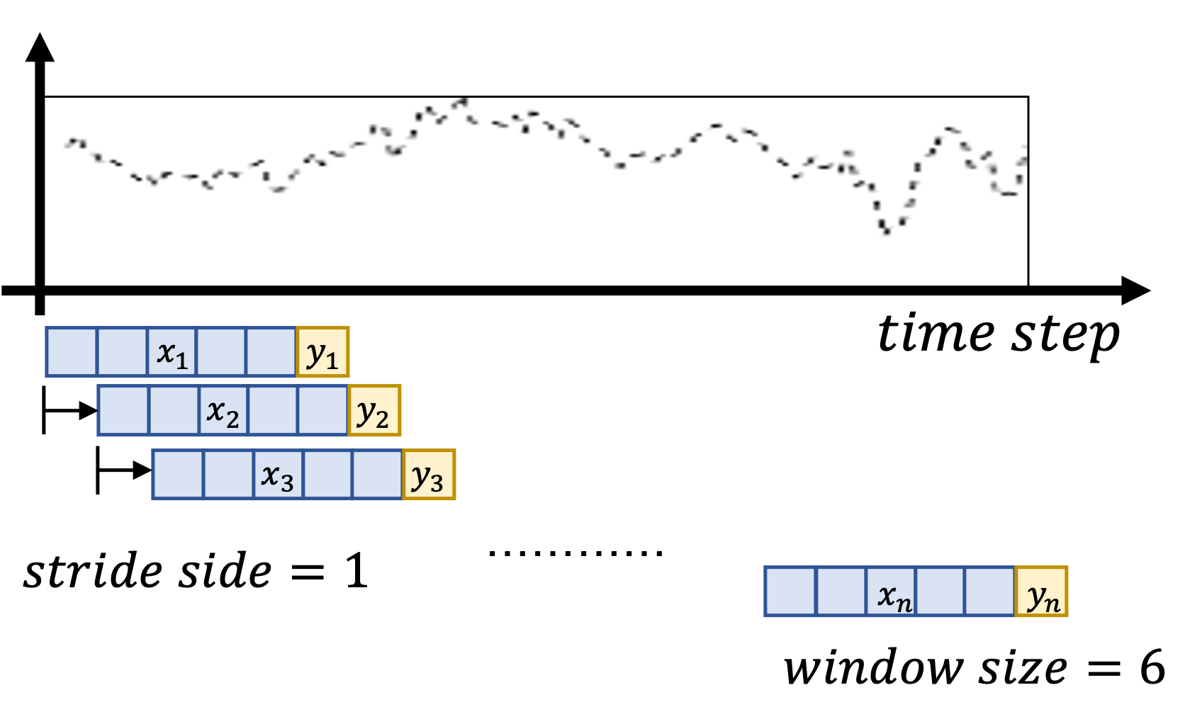
Figure 1: Illustration of the rolling forecasting setting with stride size=1.

There are two difficulties associated with applying Transformer models for M-LSTF problems. Firstly, the Transformer was originally designed for language analysis [6], which can be seen as a single series of sequential data; hence, its ability to analyze interactions between different data series is limited. As a result, the Transformer architecture can be inadequate for multivariate problems. Secondly, LSTF is more prone to overfitting than short-term forecasting because it requires models to have larger dimensions to accommodate larger input and output sizes, which leads to increased training parameters. In addition, models are trained under a rolling forecasting setting as common practice for time-series forecasting (See Figure 1 for more details). However, under the rolling forecasting setting, if the stride size is 1, then the previous and current training samples are only one data point apart from each other. Since making longer predictions typically requires longer input sequences, training samples for LSTF models have a higher degree of similarity. For example, when the model’s input length is 2, the similarity between two consecutive training inputs is 50% (1/2); however, if we increase the model’s input length to 168, the similarity between two consecutive training inputs rises to 99.4% (167/168). Therefore, the LSTF models are more likely to suffer from overfitting due to high data similarity. One could argue that we could decrease the training sample similarities by increasing the stride size; however, the number of training samples decreases by the factor of the stride size, as the training sample numbers are calculated by:

$$N_{t}=\frac{N_{d}-S_{w}+1}{S_{s}}\rm{.}$$ (1)

Where $N_{t}$ represents the number of training samples, $N_{d}$ represents the total number of time points in the training data, $S_{w}$ refers to the window size, and $S_{s}$ is the stride size. Although increasing stride sizes can decrease the sample similarities, it causes a decrease in training sample numbers, which also increase the likelihood of overfitting.

Our work specifically targets the aforementioned difficulties. To address the first problem, we focus on improving the Transformer’s ability to recognize more complicated sequential patterns from highly similar training data, thereby increasing a model’s ability to address M-LSTF problems. This is achieved by adopting a task-level memory-driven transformer approach, which both effectively utilizes the past time-series information and introduces further calculations to enhance the model’s ability on complex pattern recognition. To address the second limitation, we adopt a progressive training schedule to increase the model’s generalization power. Here, we leverage the concept of curriculum learning, whereby we gradually increase the training task difficulty and data variety by progressively introducing Bernoulli noises to the training data via a dynamic dropout scheme that can effectively reduce overfitting and increase the model performance. The main contributions of this paper are summarized as follows:

• We propose to forecast multivariate long sequence time-series data via a generalizable memory-driven transformer. This is the first work focusing on multivariate long sequence time-series forecasting to the best of our knowledge.

• We propose a task-level memory matrix to drive the forecasting process and employ a progressive training schedule to improve the generalizability of our method.

• Extensive experiments are performed, and the results show that our method can be seamlessly plugged into different transformer-based models and improve their performances.

2 Related Work

Transformer-based models have achieved state-of-the-art results in many time-series tasks [34], especially in LSTF problems [40, 39, 47, 12]. There are several areas of focus among the latter studies. Some have focused on reducing the computational costs to enable longer predictions by sparse attention, whereby the memory cost is reduced from O($L^{2}$) to as low as O($LlogL$) [40, 47], where $L$ refers to the sequence length in attention layers. Studies have also changed the architecture to further enhance the Transformer’s ability to learn time-series patterns [39]. However, all of these studies primarily focus on univariate long sequence time-series forecasting (U-LSTF) problems. Since M-LSTF problems require the model to also understand time-series interactions across multiple features, M-LSTF should be treated differently than U-LSTF.

The concept of the memory component originated from [36] where it allows the model to better remember the past inputs in NLP. Since then, this concept has been further developed by multiple researchers [42, 28]. In the recent two years, many researchers have been applying this idea on Transformer-based models across a variety of topics such as medical report generation [5], question and answer modelling [11], video captioning [15], speech recognition [30, 46] and speech translation [24] etc.. These studies suggest that the memory block is effective in reinforcing the model to learn the complicated sequential patterns. Since time-series data also have a strong sequential pattern, the memory unit should further improve the existing Transformer methods on the time-series problems.

In recent years, researchers have come up with various progressive training strategies to help models learn from complex datasets, in which the researchers design special training schedules to allow gradual improvements of models throughout their training processes. This concept has been widely used across multiple fields, such as computer vision [9, 26, 16, 17, 18, 20, 19, 45] and NLP [44]. There are many different ways of practising progressive training. An example of such practice is progressive curriculum learning (CL) defined by [31], in which it is a newer type of CL that is not directly related to sample difficulty [3], but rather entails a progressive adaption of the task setting. [25] utilized this approach in developing a “curriculum dropout" function that provides a time schedule to monotonically increase the number of model parameters expected to be suppressed based on a Bernoulli distribution; they suggest that the dropout rate should be lower at the start and progressively increase throughout the training process. Since there is a proven connection between the dropout and data noises [43], by applying such a function, we can introduce further noises to the data, which indirectly increases the prediction tasks’ difficulties over training epochs. The authors conducted extensive experiments over a range of datasets and showed that the approach can effectively address overfitting issues and increase model performance.

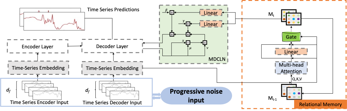
Figure 2: An overview of the model architecture. $M_{t-1}$ represents the memory matrix from the previous prediction, $M_{t}$ represents the updated memory matrix during the current sequence prediction, which in turn is recycled to be the $M_{t-1}$ for the next prediction.

3 Approach

In this section, we present our method that specifically targets the challenges for M-LSTF. Our approach is based upon the Transformer architecture; we aim to enhance Transformer models on M-LSTF problems by making improvements from both the architectural and training optimization prospects. The overview of our approach is illustrated in Figure 2. Our model comprises three major elements, namely the input embedding, the main Transformer-based model and the memory component, whereby we propose to train the model based on a progressive strategy. A description of the first two units is presented in the § 3.1, and the memory component is described in the remaining subsections.

Typical time-series models normally train under rolling forecasting settings with a fixed window and a stride size = 1, as shown in Figure 1. The input data at time t can be written as $X^{t}=\{x_{1}^{t},x_{2}^{t}...x^{t}_{\emph{L}_{S}}|x_{k}^{t}\in\rm{R}^{\emph{d}_{\emph{f}}}\}$, where ${L}_{S}$ is the input length and the feature dimension $d_{f}>1$. Moreover, the model output is $Y^{t}=\{y_{1}^{t},y_{2}^{t}...y^{t}_{\emph{L}_{p}}\}$, where ${L}_{p}$ is the prediction length, and the output feature dimension is flexible and is not limited to single sequence predictions.

3.1 Base Model

Input Embedding The input data are first passed through an embedding. Different from other types of sequential data, in time series problems, the model should capture the time information. This is extremely crucial in LSTF settings, as models are required to make predictions up to weeks in advance. We decided to utilize the time-series specific embedding method proposed by [47]. The method applies a combination of the context vector, the positional embedding and the seasonal embedding. The context vector $u^{t}\in R^{L_{S}*d_{model}}$ is obtained by projecting the model input $X^{t}\in R^{L_{S}*d_{f}}$ into a dimension of $d_{model}$ by an 1-D convolutional layer. The goal of the context vector is to transform the input data into an appropriate dimension. The positional embedding (PE(pos)) and the seasonal embedding (SE(pos)) are used to capture the local context and the global time feature, respectively. The formula for the input embedding is:

$$X_{embed}^{t}=\delta u^{t}+\rm{PE}(\rm{pos})+\sum_{k}[\rm{SE(pos)}]_{k}$$ (2)

Where $X_{embed}^{t}\in R^{L_{S}*d_{model}}$ is the embedded model input, $\delta$ is the weight factor to balance between the embeddings and the context vector and k represents the levels of the seasonal components, i.e. days, weeks, seasons, holidays.

Encoder-Decoder Architecture The backbone of our method lies on Transformer-based models following an encoder-decoder structure. Despite some minor differences between different variants, their general purpose is the same. The encoder takes past input sequences into the model and generates hidden states as outputs that contain time pattern information, which the decoder uses to make predictions. We decided to use generative-style decoding [47], which has been proven to achieve superior performances in LSTF problems and have exponentially better computational efficiency than conventional dynamic decoding [6]. The generative-style decoding generates all predictions in one step, with the decoder feeding vector $X^{t}_{feed,dec}$ presented as:

$$X^{t}_{feed,dec}=\rm{Concat}\it{(X_{dec}^{t},X_{0}^{t})}\in\it{{R^{(L_{dec}+L_{p})*d_{f}}}},$$ (3)

where $X_{dec}^{t}\in R^{L_{dec}*d_{f}}$ is the time-series input sequence for the decoder, $L_{dec}$ is the length of the decoder time-series input, $X_{0}^{t}\in R^{L_{p}*d_{f}}$ is the placeholder for the prediction sequence, and the $L_{p}$ is the prediction length.

3.2 Memory-driven Forecasting

Applications of the memory concept have demonstrated superior performances in a variety of sequential tasks [21, 22, 8]. In particular, [41] demonstrated that the memory concept is effective in improving LSTM’s ability on multivariate time-series forecasting. Therefore, this concept should also work on Transformer models under the multivariate forecasting setting. There are various ways of implementing memory into Transformers [11, 14, 7, 2, 5, 37, 23]. Our goal is to enhance the Transformer’s ability on both handling increased data complexity brought by multivariate data and recognizing hidden sequential patterns from highly similar training data. We decide to incorporate a memory unit into the decoder block because the decoder block is highly relevant to the output predictions. Our work is based on the relational memory proposed by [5], as it has proven successful in the case of medical report generation, in which reports are all highly similar and follow a strict structure. The relational memory has a self-attention layer which can help to further analyze the hidden sequential patterns that are missed by the encoder-decoder component through combining information stored in the memory matrix together with the model input. To further improve this concept, we make the relational memory unit function at a task level to suit the time-series features. The way to connect the relational memory block to the decoder is via a memory-driven conditional layer normalization (MDCLN) layer [5], the general formula for this connection can be written as:

$$\rm{MDCLN(Att(h_{l-1}),M_{t})}$$ (4)

where MDCLN(.) is the memory-driven conditional layer normalization, Att(.) represents the attention layer in the decoder block, h represents the output state from the previous layer $l-1$, and $M_{t}$ refers to the updated memory matrix at time point $t$.

Memory-driven Conditional Layer Normalization The Memory-driven Conditional Layer Normalization (MDCLN) is a way to integrate relational memory into the decoder [5] (See Figure 2 in the main article for the architecture overview), where outputs from the decoder’s self-attention layer undergoes layer normalization along with the memory information provided from the relational memory block. The reason for using layer normalization instead of batch normalization is that input data are normalized before feeding into models as common practice for time-series forecasting. Hence, instead of normalizing values among batches, we use layer normalization to normalize the features within each batch to give each time feature an equal weight for generating predictions.

In MDCLN, we update $\gamma$ and $\beta$ based on the memory matrix $M_{t}$, as they are the two most essential parameters for normalization:

$$\gamma_{t}=\gamma+\it{f_{l}(M_{t})},$$ (5)

$$\beta_{t}=\beta+f_{l}(M_{t}).$$ (6)

Where $f_{l}(.)$ represents the linear layer. The MDCLN is achieved by:

$$\rm{MDCLN}(\it{h_{l-1}},\it{M_{t}})=\gamma_{t}\odot\frac{h_{l-1}-\mu}{\sigma}+\beta_{t}+f_{l}).$$ (7)

Where $\mu$ and $\sigma$ are the mean and standard deviation of $h_{l-1}$, and $h_{l-1}$ is the output of self-attention at layer $l-1$ in the decoder.

Gate Mechanism The gate mechanism decides the proportion of new information from $\bar{M_{t}}$ to incorporate and the proportion of $M_{t-1}$ to discard to produce the final $M_{t}$. The gate mechanism has two key components: the input gate $G_{i}^{t}$ and the forget gate $G_{f}^{t}$. The two gates are calculated by balancing the embedded decoder input $X_{feed,dec}^{t-1}$ and the previous memory matrix at $t-1$ ($M_{t-1}$), where we duplicate the $embed(X_{feed,dec}^{t-1})$ to match the dimension of $M_{t-1}$. These two gates have the formulas:

$$G_{i}^{t}=embed(X_{feed,dec}^{t-1})\times W_{i}+\tanh{\left(\it{M_{t-1}}\right)}\times\ \it{U_{i}},$$ (8)

$$G_{f}^{t}=embed(X_{feed,dec}^{t-1})\times W_{f}+\tanh{\left(\it{M_{t-1}}\right)}\times\ \it{U_{f}}.$$ (9)

Where $W_{i}$, $W_{f}$, $U_{i}$, and $U_{f}$ are trainable weights for the two gates.

Table 1: The comparison of our method with the Transformer baselines, where ProbTrans is the Transformer with ProbSparse attention (three repetitions). The numbers in bold represent the better-performed models in each Transformer-based model pair.

method		Informer+ours		Informer		Transformer+ours		Transformer		Fedformer+ours		Fedformer
metric		MSE	MAE	MSE	MAE	MSE	MAE	MSE	MAE	MSE	MAE	MSE	MAE
	24	0.495	0.493	0.550	0.541	0.474	0.493	0.456	0.474	0.304	0.370	0.315	0.381
	48	0.582	0.555	0.644	0.606	0.585	0.568	0.608	0.584	0.335	0.381	0.338	0.392
Etth1	168	0.981	0.771	1.110	0.861	0.914	0.750	0.925	0.767	0.407	0.438	0.420	0.443
	336	1.098	0.816	1.237	0.893	1.001	0.801	1.077	0.821	0.451	0.454	0.459	0.465
	720	1.156	0.842	1.475	0.993	1.164	0.871	1.182	0.872	0.467	0.489	0.506	0.507
	24	0.542	0.560	0.385	0.467	0.534	0.581	0.474	0.522	0.224	0.316	0.220	0.321
	48	1.190	0.873	1.959	1.119	0.909	0.761	1.063	0.832	0.271	0.358	0.284	0.47
Etth2	168	4.869	1.856	5.957	2.036	4.951	1.807	4.067	1.623	0.405	0.410	0.412	0.427
	336	4.672	1.872	4.303	1.780	4.371	1.727	3.852	1.613	0.481	0.469	0.496	0.487
	720	3.358	1.569	3.444	1.574	3.690	1.671	2.603	1.369	0.452	0.463	0.463	0.474
	24	0.542	0.374	0.562	0.388	0.560	0.383	0.552	0.380	0.590	0.411	0.588	0.412
	48	0.650	0.435	0.692	0.447	0.679	0.440	0.698	0.448	0.694	0.459	0.686	0.457
Air	168	0.720	0.479	0.883	0.518	0.780	0.502	0.798	0.499	0.805	0.504	0.816	0.515
	336	0.773	0.505	0.852	0.536	0.789	0.501	0.823	0.514	0.827	0.515	0.834	0.518
	720	0.793	0.503	0.861	0.534	0.840	0.514	0.859	0.524	0.885	0.526	0.898	0.540
	24	0.324	0.222	0.381	0.264	0.337	0.248	0.411	0.282	0.611	0.412	0.556	0.364
	48	0.351	0.243	0.440	0.300	0.364	0.275	0.486	0.336	0.588	0.383	0.561	0.359
Traffic	168	0.405	0.300	0.567	0.396	0.407	0.300	0.555	0.384	0.60	0.374	0.612	0.381
	336	0.397	0.291	0.572	0.399	0.413	0.302	0.570	0.400	0.614	0.380	0.621	0.383
	720	0.468	0.330	0.585	0.400	0.392	0.293	0.585	0.399	0.627	0.381	0.626	0.382
	24	0.253	0.338	0.258	0.342	0.253	0.340	0.263	0.352	0.148	0.231	0.162	0.247
	48	0.344	0.411	0.354	0.418	0.338	0.414	0.348	0.419	0.189	0.274	0.204	0.293
Weather	168	0.507	0.520	0.578	0.544	0.513	0.512	0.551	0.526	0.263	0.325	0.284	0.347
	336	0.545	0.537	0.591	0.553	0.512	0.507	0.584	0.547	0.335	0.376	0.349	0.390
	720	0.593	0.567	0.625	0.643	0.554	0.530	0.642	0.576	0.404	0.415	0.413	0.428

Task-level Memory Matrix In addition to the further calculations that the relational memory unit can bring, another main characteristic of this unit is that it can read/write information from/to a memory matrix which assists with analyzing time patterns. In NLP problems, we use dynamic decoding [6]; the memory matrix works by maintaining information from the prediction of the last token/word while predicting a paragraph, and this matrix is re-initialized after each paragraph, as each paragraph is perceived as being independent [5]. However, as explained above, we use generative-style decoding for our task, in which it generates all predictions in a single step [47]. In this case, the traditional matrix initialization method will not work, as we do not generate individual time point predictions one by one. In addition, for each forecasting problem, the input sequences for making previous predictions are still helpful for any future prediction, as they come from the same time series and share similar pattern interactions. Therefore, we adjust the matrix initialization method to a task level. We maintain a memory matrix for each specific forecasting task, where we keep the matrix output from the relational memory at the prediction time point $t-1$ as the input matrix at time point $t$; this matrix is updated after every prediction by a gating mechanism to control the ratio of the memory matrix being updated. Since more recent model inputs are weighted higher than those from the distant past, the matrix can maintain all relevant time information. In addition, this matrix will continue updating even after training, which ultimately increases the model’s generalization power. The relational memory unit updates the memory matrix by first calculating the self-attention based on the matrix $M$ at time point $t-1$, where $\rm{Q}=\it{M_{t-1}}\rm{\times\ W_{q}}$, $\rm{K}=\rm{[\it{M_{t-1}};\ embed(X_{feed,dec}^{t})]\times\ \rm{W_{k}}}$ and $\rm{V=[\it{M_{t-1}};\ embed(X_{feed,dec}^{t})]}\times\ \rm{W_{v}}$. The $\rm{W_{k}}$, $\rm{W_{v}}$ and $\rm{W_{q}}$ are trainable weights, and $[M_{t-1};\rm{embed}(X_{feed,dec}^{t})]$ is the row-wise concatenations between $M_{t-1}$ and the embedded decoder feeding vector. We then calculate the self-attention score $Z$ from Q, K and V. After the self-attention layer, we go through a feedforward layer to produce $\bar{M_{t}}$, which is calculated as:

$$\bar{M_{t}}=\rm{Feedforward}\it{(Z+M_{t-1})+Z+M_{t-1}}$$ (10)

$\bar{M_{t}}$ is then passed through a gating mechanism to calculate the ratio of the $\bar{M_{t}}$ to be added to the final $M_{t}$:

$$M_{t}=\sigma\left(G_{f}^{t}\right)\ \odot\ M_{t-1}+\sigma\left(G_{i}^{t}\right)\ \odot\ \bar{M_{t}}\rm{,}$$ (11)

where $G_{i}^{t}$ is the input gate, $G_{f}^{t}$ is the forget gate, $\odot$ is the Schur product, and $\sigma(.)$ is the sigmoid function.

3.3 Generalizable Progressive Training

Overfitting is one of the main drawbacks of M-LSTF models due to the increased model dimension and a high degree of the training sample similarity. The increased model dimension is unavoidable, as the model input and output must increase when predicting long sequence predictions. Therefore, we decided to mitigate the problem from the training sample perspective under the rolling forecasting setting. However, as mentioned in the introduction, increasing stride size for the rolling window does not help with the overfitting issue. We decided to target the overfitting issue by adding sample variety. These noises should be added in a manner such that the rate is slower at the beginning to ensure that the model has a good grasp of the data pattern before we start to increase the rate of introducing noises to prevent the model from overfitting. To achieve this goal, we decided to alter dropout rates, as there is a proven connection between dropout and noises [4, 33, 43]. We dynamically alter the dropout rate during training based on a monotone function proposed by [25], whereby the function rate starts slower and later increases as training proceeds. The dropout rate function is based on:

$$\theta_{d}(t)=\min(\theta_{max},1-\theta_{max}-{(1-\theta}_{max})\exp(-\gamma t))$$ (12)

where t is the $t^{th}$ number of 100 iterations, $\theta_{d}$ is the dropout rate, $\theta_{max}$ is the maximum dropout rate, and $\gamma$ is a hyper-parameter typically set between 0.001 to 0.01.

Loss Function The loss function we use is Mean Squared Error (MSE) loss on the target sequences, and it is then back propagated across the entire network.

$$L_{MSE}=\frac{1}{n}\sum_{i=1}^{n}(y_{i}-\hat{y_{i}})^{2}$$ (13)

where $y_{i}$ is the true value for the $i^{th}$ time step in the output sequence, $\hat{y_{i}}$ is the predicted value, and n is the total number of values. Both $y_{i}$ and $\hat{y_{i}}$ have a dimension of $\geq{1}$.

4 Experiments

4.1 Datasets

We conduct extensive experiments on 5 public benchmark datasets.

ETT (Electricity Transformer Temperature) [47]. The dataset contains information about six power load features and the target value “oil temperature”. We use the two hourly datasets from the source named as $\rm{Etth_{1}}$ and $\rm{Etth_{2}}$. We use the first 20 months of data and the train/val/test splits follow the ratio of 6/2/2.

Weather (Local Climatological Data) . The dataset contains hourly data about climate information from around 1,600 locations in USA between 2018 and 2020. The data consist of seven quantitative climatological features with “dry builb temperature” as the target. The train/val/test ratio is 7/1/2.

Air Quality (Beijing Multi-site Air-Quality Data). The dataset consists of eleven quantitative hourly features relevant to air quality with the target value set as “PM10” from 12 national air quality monitoring sites. We use the data from the “Wanshouxigong” station. The train/val/test follows the ratio of 7/1/2.

Traffic (Metro Interstate Traffic Volume) . The dataset contains the traffic condition data measured in the of between Minneapolis and St Paul, Minnesota, USA. The datasets has five hourly numerical features with the target value of “traffic volume". The train/val/test follows the ratio of 7/1/2.

4.2 Experimental Details

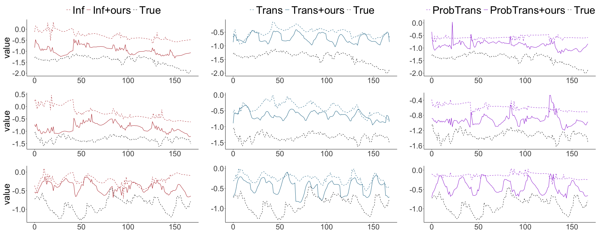
Figure 3: The test results of applying our proposed memory unit to different Transformer-based models on the Etth1 dataset with the prediction length of 168.

Baselines We use three Transformer variants as our baseline with generative-style decoding to generate the output sequences in one step [48, 47]. The three Transformer-based models are the Transformer model with canonical attention, the Transformer model with ProbSparse attention, the Fedformer [48] and the Informer model [47]. In addition, we compared our model’s performance with two classical DNN time-series methods: the LSTM [1] and LSTnet [13].

Table 2: Key parameters for transformer-based models.

Prediction Len.	{24,48}	{168,336}	{720}
$d_{model}$	1024	1024	1024
$d_{ff}$	2048	2048	2048
n_heads	8	8	8
Dropout	0.1	0.1	0.1
Activation	GELU	GELU	GELU
Batch Size	32	8	4
Enc.Layer no.	1	2	2
Dec.Layer no.	1	1	1

Table 3: Key parameters for the relational memory unit.

	Informer	Fedformer	ProbTrans
$d_{rm}$	1024	1024	1024
Mem.slot.no.	1	1	2
Mem.head.no.	4	2	2

Implementation Details Our model is constructed based on Pytorch with Python 3.7. We use a single NVIDIA Tesla V100 GPU for training. All of the input data undergo normalization before being fed into the model. The training is performed under the rolling forecasting setting (stride size=1). The encoder and decoder input lengths are {48,96,168,168,336} and {48,48,168,168,336}, which correspond to the prediction lengths of {24,48,168,336,720}, respectively. For the progressive training scheme, we update the dropout rate for every 100 iterations with the upper dropout limit of 0.1. Moreover, we apply early stopping technique with patience=3 during training and the training epoch is set to be 6. The learning rate starts from 0.0001 and it halves its value for every epoch after the first two epochs.

Model Reproducibility To ensure the model reproducibility, we present detailed parameter settings in this section. Table 2 describes the details for all Transformer-based models. We use the same setting for all three Transformer-based models in our experiment because these three models share a very similar structure and show optimal performance under similar settings. However, we use different settings for different prediction output lengths to adjust the model for different prediction tasks. Table 2 specifies the model dimension ($d_{model}$), the dimension of positional feedforward layers inside the encoder and decoder block ($d_{ff}$), and the number of attention heads in each attention layer (n_heads). In addition, we include information about batch size, layer activation function, the encoder layer number (Enc.Layer no.), and the decoder layer number (Dec.Layer no.). Table 3 describes the parameters for the relational memory block. There are three key parameters for the relational memory unit: the unit dimension ($d_{rm}$), the number of memory units (Mem.slot.no), and the number of attention heads in the relational memory (Mem.head.no). Here, we apply different relational memory settings for the three Transformer-based models as they require different settings to achieve optimal performance.

Evaluation Metrics We use two evaluation metrics to measure our model performance: Mean Squared Error (MSE) and Mean Absolute Error (MAE).

4.3 Results and Analysis

Comparison with baselines Table 1 summarizes the results of the Transformer baselines and our proposed methods. We applied the same setting for each transformer-based model pair to achieve a fair comparison. Based on the results in Table 1, we find that: (1) Our model can significantly improve the Transformer-based model’s performance up to 30% on M-LSTF problems across most cases; it improves the MSE and MAE scores in 23 of 25 prediction tasks in Informer, 20 of 25 tasks in Transformer with canonical attention, and 20 of 25 tasks in Transformer with ProbSparse attention. Our results show that our proposed memory-driven approach with the progressive training schedule can help Transformers with M-LSTF problems. (2) Our method works particularly well in longer prediction settings. For instance, when the prediction length is 720, our approach improves the Informer’s MSE score by 21.63% for the Etth1 dataset and 20.00% for the traffic dataset, in contrast to the 10.00% and 14.96% improvements, respectively, for the prediction length of 24, and this trend is consistently observed across all different models and datasets. The improved performance with longer prediction settings makes sense, considering that the relational memory unit is highly effective at dealing with highly similar data, and our progressive training strategy effectively addresses the overfitting issues caused by increased prediction lengths. (3) Our method can further improve the performances of the SOTA LTF model, Fedformer, on almost all the tasks. Such experimental results prove that our method can be seamlessly plugged into any Transformer-based models even when these models are designed to explore the global and seasonal-trend features to improve the prediction capabilities. The frequency modules in Fedformer can be considered as another kinds of memory-driven paradigm, and it is encouraged to observe that our methods bring out additional improvements.

Table 4: Comparison of our method with other DNN methods on Multivariate Long Sequence Time.

Methods		Informer+ours		LSTM		LSTnet
Metrics		MSE	MAE	MSE	MAE	MSE	MAE
Etth1	24	0.495	0.493	0.650	0.624	1.293	0.901
	48	0.582	0.555	0.702	0.675	1.456	0.960
	168	0.981	0.771	1.212	0.867	1.997	1.214
	336	1.098	0.816	1.424	0.994	2.655	1.369
	720	1.156	0.842	1.960	1.322	2.143	1.380
Etth2	24	0.542	0.560	1.143	0.813	2.742	1.457
	48	1.190	0.873	1.671	1.221	3.567	1.687
	168	4.869	1.856	4.117	1.674	3.242	2.513
	336	4.672	1.872	3.434	1.549	2.544	2.581
	720	3.358	1.569	3.963	1.778	4.625	3.709

Table 5: Ablation study for the decomposition of our approach, where p.t. is the progressive training scheme and mem refers to our memory approach (three repetitions).

datasets		Etth1				Air quality				Traffic
prediction		24	48	168	336	24	48	168	336	24	48	168	336
Informer	MSE	0.550	0.644	1.110	1.237	0.562	0.692	0.833	0.852	0.381	0.440	0.567	0.572
	MAE	0.541	0.606	0.861	0.893	0.388	0.447	0.518	0.536	0.264	0.300	0.396	0.399
Informer + p.t.	MSE	0.510	0.651	1.021	1.136	0.583	0.690	0.813	0.848	0.377	0.431	0.564	0.571
	MAE	0.514	0.608	0.820	0.820	0.387	0.447	0.524	0.535	0.262	0.290	0.389	0.398
Informer + mem	MSE	0.510	0.588	1.009	1.161	0.569	0.680	0.769	0.794	0.331	0.352	0.411	0.417
	MAE	0.506	0.556	0.810	0.827	0.386	0.438	0.496	0.516	0.228	0.249	0.302	0.306
Informer + ours	MSE	0.495	0.582	0.981	1.098	0.542	0.650	0.720	0.773	0.324	0.351	0.405	0.397
	MAE	0.493	0.555	0.771	0.816	0.374	0.435	0.479	0.505	0.222	0.243	0.300	0.291

Table 6: Ablation study of different memory matrix initialization methods (three repetitions).

datasets		Etth1				Etth2				Weather
prediction		24	48	336	720	24	48	168	336	24	48	168	336
Informer+mem	MSE	0.510	0.588	1.009	1.161	0.553	1.204	5.069	4.883	0.243	0.350	0.519	0.556
(Ours)	MAE	0.506	0.556	0.810	0.843	0.578	0.879	2.043	1.896	0.328	0.411	0.525	0.549
Informer+mem	MSE	0.537	0.571	1.168	1.224	0.592	1.242	6.454	5.034	0.254	0.353	0.521	0.567
(Original)	MAE	0.528	0.546	0.848	0.894	0.602	0.888	2.251	1.943	0.335	0.412	0.530	0.544

Apart from the Transformer baselines, in Table 4, we also compare our methods with the prediction results from two classical time-series deep neural network (DNN) methods, namely the LSTM and LSTnet, from [47]. We can see the Informer+ours method outperforms LSTM and LSTnet in all tasks in the Etth1 dataset and 3 of the 5 prediction tasks in the Etth2 dataset. When the prediction length is 720, the Informer+ours method achieves a 41.02% and 36.79% improvement on the MSE and MAE scores over LSTM and a 46.05% and 38.98% improvement on the MSE and MAE scores over LSTnet for the Etth1 dataset. For the Etth2 dataset, we also observe a substantial improvement of up to 57.70% on the MSE and MAE scores when using our proposed approach. Although LSTM and LSTnet perform better with the Etth2 dataset than our approach, this could be due to the differences caused by the datasets, which is extremely common in time-series forecasting [29, 47]. Such variations could be explained by the “no free lunch theorem" [38], as different time-series data can have completely distinct patterns, it is extremely difficult to create a model that fits all kinds of data. Overall, our approach demonstrates remarkable improvements over the classical DNN methods in most settings.

Case Study Figure 3 is a visualization of time series predictions by different models on the Etth1 dataset. Based on these plots, we can observe that the proposed memory unit can better maintain short-term fluctuations or the seasonal component of data. In particular, in the case of the Transformer with ProbSparse attention, we can see that the memory unit helps the model to capture the seasonal component very well, such that the short-term fluctuations are better captured by the model with the proposed memory unit, in contrast to the predictions for the model without the memory unit, for which the trend line stays relatively smooth and does not vary much across time. This result demonstrates that our relational memory block is able to detect patterns from highly similar data and is very sensitive to small data changes, which enhances the model’s ability to learn from the seasonal component of the time-series data. Additionally, based on Figure 3, most of our proposed approach’s predictions are closer to the true values than their base model’s predictions, reflecting our proposed approach’s superiority. In addition, we can see that our approach is better at capturing the short-term fluctuations than the Transformer-based models, as the prediction trend lines for the Transformer-based models are smoother and does not vary much across time, which demonstrates that our model can detect more minor data changes.

Ablation Study We performed two ablation studies to better understand the performance of our model. We first ran experiments on the Etth1, Air Quality and Traffic dataset and compared the performance of the different components of our proposed methods. We summarize the results in Table 5, we can see that both the progressive training strategy and the relational memory unit are individually able to enhance the Informer performance to a certain extent; however, the extent of the improvement is less than when they are combined, thereby indicating that our approach can make effective use of the two components. In addition, each of the components is more effective in the longer sequence settings, thereby suggesting that they are both capable of addressing the difficulties associated with LSTF problems.

Table 6 demonstrates the results of our second ablation study, in which we studied the effectiveness of our task-level memory matrix. The first row shows the results of the Informer with the relational memory block that uses our task-level memory matrix, and the second row represents the Informer with the relational memory block that uses the original memory matrix [5]. The results show that our proposed memory matrix approach outperforms the original matrix in both MSE and MAE scores in 11 of 12 prediction tasks, thereby demonstrating that the adaptations we made for the memory matrix can enhance the performance of our relational memory block.

5 Conclusion

In this paper, we propose a generalizable memory-driven approach targeting M-LSTF. Our approach is designed to target the specific data characteristics of M-LSTF datasets. We train a task-level memory-driven Transformer-based model in a progressive fashion. We demonstrate that the task-level memory improves the model’s ability to comprehend the multivariate sequential patterns from highly similar training samples. In addition, the progressive training schedule can effectively address overfitting issues in LSTF. We validated our methods on five different publicly available datasets with five different prediction lengths ranging from 24 to 720 time steps. The results show that our method works exceptionally well with longer prediction sequences and can achieve up to 30% improvement. Lastly, it is worth noting that to the best of our knowledge, this is the first study that focuses on addressing the particular challenges that arise from M-LSTF.

References

- [1] Dzmitry Bahdanau, Kyunghyun Cho, and Yoshua Bengio, ‘Neural machine translation by jointly learning to align and translate’, in ICLR, (2015).
- [2] Andrea Banino, Adrià Puigdomènech Badia, Raphael Köster, Martin J. Chadwick, Vinícius Flores Zambaldi, Demis Hassabis, Caswell Barry, Matthew Botvinick, Dharshan Kumaran, and Charles Blundell, ‘MEMO: A deep network for flexible combination of episodic memories’, in ICLR, (2020).
- [3] Yoshua Bengio, J. Louradour, Ronan Collobert, and J. Weston, ‘Curriculum learning’, in ICML, (2009).
- [4] Charles M. Bishop, ‘Training with noise is equivalent to tikhonov regularization’, Neural Computation, 7, 108–116, (1995).
- [5] Zhihong Chen, Yan Song, Tsung-Hui Chang, and Xiang Wan, ‘Generating radiology reports via memory-driven transformer’, in EMNLP, (2020).
- [6] J. Devlin, Ming-Wei Chang, Kenton Lee, and Kristina Toutanova, ‘Bert: Pre-training of deep bidirectional transformers for language understanding’, in NAACL, (2018).
- [7] Kuan Fang, Alexander Toshev, Fei-Fei Li, and Silvio Savarese, ‘Scene memory transformer for embodied agents in long-horizon tasks’, in CVPR, (2019).
- [8] Zhengcong Fei, ‘Memory-augmented image captioning’, in AAAI, (2021).
- [9] Negar Heidari and Alexandros Iosifidis, ‘Progressive graph convolutional networks for semi-supervised node classification’, IEEE Access, 9, 81957–81968, (2021).
- [10] S. Hochreiter and J. Schmidhuber, ‘Long short-term memory’, Neural Computation, 9, 1735–1780, (1997).
- [11] Ming Jiang, Junlei Wu, Xiangrong Shi, and Min Zhang, ‘Transformer based memory network for sentiment analysis of web comments’, IEEE Access, 7, 179942–179953, (2019).
- [12] Ming Jin, Guangsi Shi, Yuan-Fang Li, Qingsong Wen, Bo Xiong, Tian Zhou, and Shirui Pan, ‘How expressive are spectral-temporal graph neural networks for time series forecasting?’, arXiv preprint arXiv:2305.06587, (2023).
- [13] Guokun Lai, Wei-Cheng Chang, Yiming Yang, and Hanxiao Liu, ‘Modeling long- and short-term temporal patterns with deep neural networks’, ACM SIGIR, (2018).
- [14] Guillaume Lample, Alexandre Sablayrolles, Marc’Aurelio Ranzato, Ludovic Denoyer, and H. Jégou, ‘Large memory layers with product keys’, in NeurIPS, (2019).
- [15] Jie Lei, Liwei Wang, Yelong Shen, Dong Yu, Tamara L. Berg, and Mohit Bansal, ‘MART: memory-augmented recurrent transformer for coherent video paragraph captioning’, in ACL, (2020).
- [16] Mingjie Li, Wenjia Cai, Rui Liu, Yuetian Weng, Xiaoyun Zhao, Cong Wang, Xin Chen, Zhong Liu, Caineng Pan, Mengke Li, et al., ‘Ffa-ir: Towards an explainable and reliable medical report generation benchmark’, in Thirty-fifth Conference on Neural Information Processing Systems Datasets and Benchmarks Track (Round 2).
- [17] Mingjie Li, Wenjia Cai, Karin Verspoor, Shirui Pan, Xiaodan Liang, and Xiaojun Chang, ‘Cross-modal clinical graph transformer for ophthalmic report generation’, in Proceedings of the IEEE/CVF Conference on Computer Vision and Pattern Recognition, pp. 20656–20665, (2022).
- [18] Mingjie Li, Po-Yao Huang, Xiaojun Chang, Junjie Hu, Yi Yang, and Alex Hauptmann, ‘Video pivoting unsupervised multi-modal machine translation’, IEEE Transactions on Pattern Analysis and Machine Intelligence, (2022).
- [19] Mingjie Li, Bingqian Lin, Zicong Chen, Haokun Lin, Xiaodan Liang, and Xiaojun Chang, ‘Dynamic graph enhanced contrastive learning for chest x-ray report generation’, arXiv preprint arXiv:2303.10323, (2023).
- [20] Mingjie Li, Rui Liu, Fuyu Wang, Xiaojun Chang, and Xiaodan Liang, ‘Auxiliary signal-guided knowledge encoder-decoder for medical report generation’, World Wide Web, 26(1), 253–270, (2023).
- [21] Chao Ma, Chunhua Shen, Anthony R. Dick, Qi Wu, Peng Wang, Anton van den Hengel, and Ian D. Reid, ‘Visual question answering with memory-augmented networks’, in CVPR, (2018).
- [22] Chen Ma, Liheng Ma, Yingxue Zhang, Jianing Sun, X. Liu, and M. Coates, ‘Memory augmented graph neural networks for sequential recommendation’, in AAAI, (2020).
- [23] Xutai Ma, Yongqiang Wang, Mohammad Javad Dousti, Philipp Koehn, and Juan Pino, ‘Streaming simultaneous speech translation with augmented memory transformer’, in ICASSP, (2021).
- [24] Xutai Ma, Yongqiang Wang, Mohammad Javad Dousti, Philipp Koehn, and Juan Miguel Pino, ‘Streaming simultaneous speech translation with augmented memory transformer’, in ICASSP, (2021).
- [25] Pietro Morerio, Jacopo Cavazza, Riccardo Volpi, R. Vidal, and Vittorio Murino, ‘Curriculum dropout’, in ICCV, (2017).
- [26] Bo Pang, Gao Peng, Yizhuo Li, and Cewu Lu, ‘Pgt: A progressive method for training models on long videos’, in CVPR, pp. 11379–11389, (June 2021).
- [27] Yao Qin, Dongjin Song, Haifeng Chen, Wei Cheng, Guofei Jiang, and Garrison W. Cottrell, ‘A dual-stage attention-based recurrent neural network for time series prediction’, in IJCAI, (2017).
- [28] Adam Santoro, R. Faulkner, David Raposo, Jack W. Rae, Mike Chrzanowski, T. Weber, Daan Wierstra, Oriol Vinyals, Razvan Pascanu, and T. Lillicrap, ‘Relational recurrent neural networks’, in NeurIPS, (2018).
- [29] Zhipeng Shen, Yuanming Zhang, Jiawei Lu, Jun Xu, and Gang Xiao, ‘Seriesnet:a generative time series forecasting model’, in IJCNN, (2018).
- [30] Yangyang Shi, Yongqiang Wang, Chunyang Wu, Ching feng Yeh, Julian Chan, Frank Zhang, Duc Le, and M Seltzer, ‘Emformer: Efficient memory transformer based acoustic model for low latency streaming speech recognition’, in ICASSP, (2021).
- [31] Petru Soviany, Radu Tudor Ionescu, Paolo Rota, and N. Sebe, ‘Curriculum learning: A survey’, arXiv: 2101.10382, (2021).
- [32] Ashish Vaswani, Noam Shazeer, Niki Parmar, Jakob Uszkoreit, Llion Jones, Aidan N Gomez, Łukasz Kaiser, and Illia Polosukhin, ‘Attention is all you need’, in NeurIPS, (2017).
- [33] Stefan Wager, Sida I. Wang, and Percy Liang, ‘Dropout training as adaptive regularization’, in NeurIPS, (2013).
- [34] Qingsong Wen, Tian Zhou, Chaoli Zhang, Weiqi Chen, Ziqing Ma, Junchi Yan, and Liang Sun, ‘Transformers in time series: A survey’, arXiv preprint arXiv:2202.07125, (2022).
- [35] Ruofeng Wen, Kari Torkkola, Balakrishnan Narayanaswamy, and Dhruv Madeka, ‘A multi-horizon quantile recurrent forecaster’, arXiv:1711.11053, (2018).
- [36] Jason Weston, Sumit Chopra, and Antoine Bordes, ‘Memory networks’, in ICLR, (2015).
- [37] Peratham Wiriyathammabhum, ‘Spotfast networks with memory augmented lateral transformers for lipreading’, in NeurIPS, (2020).
- [38] David H. Wolpert, ‘The lack of A priori distinctions between learning algorithms’, Neural Comput., 8(7), 1341–1390, (1996).
- [39] Haixu Wu, Jiehui Xu, Jianmin Wang, and Mingsheng Long, ‘Autoformer: Decomposition transformers with auto-correlation for long-term series forecasting’, arXiv:2106.13008, (2021).
- [40] Sifan Wu, Xi Xiao, Qianggang Ding, P. Zhao, Ying Wei, and Junzhou Huang, ‘Adversarial sparse transformer for time series forecasting’, in NeurIPS, (2020).
- [41] Dongkuan Xu, Wei Cheng, Bo Zong, Dongjin Song, Jingchao Ni, Wenchao Yu, Yanchi Liu, Haifeng Chen, and Xiang Zhang, ‘Tensorized lstm with adaptive shared memory for learning trends in multivariate time series’, in AAAI, (2020).
- [42] Jichuan Zeng, Jing Li, Yan Song, Cuiyun Gao, Michael R. Lyu, and Irwin King, ‘Topic memory networks for short text classification’, in EMNLP, (2018).
- [43] Shuangfei Zhai and Zhongfei Zhang, ‘Dropout training of matrix factorization and autoencoder for link prediction in sparse graphs’, in SDM, (2015).
- [44] Minjia Zhang and Yuxiong He, ‘Accelerating training of transformer-based language models with progressive layer dropping’, in NeurIPS, (2020).
- [45] Zenghui Zhang, Weiwei Guo, Mingjie Li, and Wenxian Yu, ‘Gis-supervised building extraction with label noise-adaptive fully convolutional neural network’, IEEE Geoscience and Remote Sensing Letters, 17(12), 2135–2139, (2020).
- [46] Yingzhu Zhao, Chongjia Ni, Cheung-Chi Leung, Shafiq R. Joty, Eng Siong Chng, and Bin Ma, ‘Speech transformer with speaker aware persistent memory’, in ISCA, (2020).
- [47] Haoyi Zhou, Shanghang Zhang, Jieqi Peng, Shuai Zhang, Jianxin Li, Hui Xiong, and Wancai Zhang, ‘Informer: Beyond efficient transformer for long sequence time-series forecasting’, in AAAI, (2021).
- [48] Tian Zhou, Ziqing Ma, Qingsong Wen, Xue Wang, Liang Sun, and Rong Jin, ‘Fedformer: Frequency enhanced decomposed transformer for long-term series forecasting’, in International Conference on Machine Learning, pp. 27268–27286. PMLR, (2022).