Distributed Safe Learning and Planning for Multi-robot Systems
Abstract
This paper considers the problem of online multi-robot motion planning with general nonlinear dynamics subject to unknown external disturbances. We propose dSLAP, a distributed Safe Learning And Planning framework that allows the robots to safely navigate through the environments by coupling online learning and motion planning. Gaussian process regression is used to online learn the disturbances with uncertainty quantification. The safe motion planning algorithm ensures collision avoidance against the learning uncertainty and utilizes set-valued analysis to achieve fast adaptation in response to the newly learned models. A model predictive control problem is then formulated and solved to return a control policy that balances between actively exploring the unknown disturbances and reaching goal regions. Sufficient conditions are established to guarantee the safety of the robots in the absence of backup policy. Monte Carlo simulations are conducted for evaluation.
I Introduction
Intelligent multi-robot systems are becoming ubiquitous in our life, such as autonomous driving, delivery, precision agriculture and search-and-rescue. Robots operating in the real world are usually accompanied by unknown disturbances. In order to guarantee the safety of the robots as well as mission completion, it is crucial for the robots being able to adapt to the disturbances online and update their motion plans accordingly.
Motion planning is a fundamental problem in robotics, and it aims to generate a series of low-level specifications for a robot to move from one point to another [1]. In the real world, robots’ operations are usually accompanied by uncertainties, e.g., from the environments they operate in and from the errors in the modeling of robots’ dynamics. To deal with the uncertainties and ensure safety, i.e., collision avoidance, existing methods leverage techniques in robust control, e.g., [2, 3, 4], stochastic control, e.g., [5, 6, 7], and learning-based control e.g., [8, 9, 10, 11]. Robust control-based approaches model the uncertainties as bounded sets and synthesize control policies that tolerate all the uncertainties in the sets. Note that considering all possible events can result in over-conservative policies whereas extreme events may only take place rarely. Stochastic control-based approaches model the uncertainties as known probability distributions. The generated motion plans enforce chance constraints, i.e., the probability of collision is less than a given threshold. On the other hand, learning-based approaches relax the need of prior explicit uncertainty models by directly learning the best mapping from sensory inputs to control inputs from repetitive trials. Paper [11] leverages PAC-Bayes theory to provide guarantees on expected performances over a distribution of environments.
The aforementioned approaches can all be classified as offline approaches where control policies are synthesized before the deployment of the robots. When robots encounter significant changes of environments during online operation, online learning of the uncertainties is desired to ensure safe arrival to the goals. Recently, a class of methods on safe learning and control have been developed to safely steer a system to a goal region while learning uncertainties online. These approaches usually adopt a switching strategy between a learning-based controller, which updates online in light of new observations, and a backup safety controller, which is suboptimal but can guarantee safety. The backup safety controllers can be synthesized through solving a two-player zero-sum differential game [12], model predictive control (MPC) [13][14], control barrier function [15, 16], robust optimization [17], reachability analysis [18] and regions of attraction [19]. The aforementioned papers only consider single-robot systems and static state constraints (e.g., static obstacles). In multi-robot systems, from the perspective of each single robot and when centralized planning is not used, the state constraints are dynamic due to the motion of the other robots, analogous to moving obstacles.
Motion planning problems are known to be computationally challenging even for single-robot systems. Paper [20] shows that the generalized mover’s problem is PSPACE-hard in terms of degrees of freedom. Multi-robot motion planning is an even more challenging problem as the computation complexity scales up by the number of robots. Centralized planners [21][22] consider all the robots as a single entity such that methods for single-robot motion planning can be directly applied. However, as [21] points out, its worst-case computation complexity grows exponentially with the number of robots. Consequently, distributed methods are developed to address the scalability issue. Most of these methods are featured with each robot conducting a single-robot motion planning strategy but coupled with a coordination scheme to resolve conflicts. These works can be categorized as fully synthesized design or switching-based design. A fully synthesized design [23][24] incorporates simple collision avoidance methods, such as artificial potential field, into the decoupled solution. Under switching-based design, a switching controller is developed such that each robot executes a nominal controller synthesized in a decoupled manner but switches to a local coordination controller when it is close to other robots [25, 26, 27]. Prioritized planning, where a priority is assigned to the robots such that robots with lower priority make compromises for the robots with higher priority, is further adopted to reduce the need of coordination [28][29]. There have been recent works which study dynamic and environmental uncertainties in multi-robot motion planning. For example, robust control-based approaches are studied in [30][31], and stochastic control-based approaches are studied in [32][33][34]. In [35][36], deep reinforcement learning is applied to train multiple robots to avoid collisions in an offline manner when explicit uncertainty models are not available. In this paper, we consider learning the uncertainties in an online fashion with data collected sequentially on the robots’ trajectories.
Contribution statement. We consider the problem of online multi-robot motion planning with general nonlinear dynamics subject to unknown external disturbances. We propose dSLAP, the distributed Safe Learning And Planning framework, where the robots collect streaming data to online learn about the disturbances, use the learned model to compute a set of safe actions that avoid collisions against the learning uncertainty, and then choose an action that balances between reaching the goals and actively exploring the disturbances. Our contribution is summarized as follows:
-
•
We propose dSLAP, a distributed two-stage motion planner. It utilizes set-valued analysis to allows for fast adaptation to the sequence of dynamic models resulted from online learning. The planner first constructs a directed graph through connecting a robot’s one-step forward sets, and then obtains a set of safe control inputs by removing the control inputs leading to collisions. Then a distributed model predictive controller selects safe control inputs balancing moving towards the goals and actively learning the disturbances.
-
•
Our two-stage motion planning is in contrast to the classic formulation [37][38] of optimal multi-robot motion planning, whose solutions solve collision avoidance and optimal arrival simultaneously and are known to be computationally challenging (PSPACE-hard [20]). Instead, dSLAP first solves for collision avoidance and then for optimal arrival. The worst-case onboard computational complexity of each robot grows linearly with respect to the number of the robots.
-
•
We derive sufficient conditions to guarantee the safety of the robots in the absence of backup policies.
Monte Carlo simulation is conducted for evaluations.
Distinction statement. This paper substantially distinguishes from the preliminary version [39] in the following aspects: (i) Detailed and structured proofs of theoretical results are included in Section IV. The proofs show how collision avoidance is achieved through the dSLAP framework, how safety is related to the number of robots and the initial conditions of the robots. (ii) A new set of theoretical results on the all-time safety of the system is provided in Theorem III.3. It provides guidance on the design of the algorithm, requirements on the computation speed of the robots and the implication on the density of the robots. (iii) Section III-E includes additional discussions on the verification of the initial condition, the comparison of the two theorems and the computation complexity of the algorithm. (iv) Additional simulation results are provided in Figure 3.
Notations. We use superscript to distinguish the local values of robot . Define the distance metric , the point-to-set distance as for a set , the closed ball centered at with radius as , and shorthand the closed unit ball centered at with radius . Let be the space of integers and the space of natural number. Denote the cardinality of a set as .
Below are the implementations of common procedures. Element removal: Given a set and an element , procedure Remove removes element from ; i.e., . Element addition: Given a set and an element , procedure Add appends to , i.e., . Nearest neighbor: Given a state and a finite set , Nearest chooses a state in that is closest to ; i.e., picks , where .
II Problem Formulation
In this section, we introduce the model of the multi-robot system, describe the formulation of the motion planning problem, and state the objective of this paper.
Mobile multi-robot system. Consider a network of robots . The dynamic system of each robot is given by the following differential equation:
| (1) |
where is the state of robot at time , is its control input, denotes the system dynamics of robot , and represents the external unknown disturbance. We impose the following assumption:
Assumption II.1.
-
(A1)
(Lipschitz continuity). The system dynamics and the unknown disturbance are Lipschitz continuous.
-
(A2)
(Compactness). Spaces and are compact.
Assumption (A1) implies that is Lipschitz continuous. Choose constant , which is larger than the Lipschitz constant of and constant , which is larger than the supremum of over and . Usually these constants can be estimated. For example, by the Bernoulli equation [40], the variation and magnitude of wind speed can be bounded due to the limited variation in temperature and air pressure.
Motion planning. We denote closed obstacle region by , goal region by , and free region at time by , where and is the radius of an overestimation of the robot size. Each robot aims to synthesize a feedback policy such that the solution to system (1) under satisfies , , , where is the first time when robot reaches . That is, each robot needs to reach the goal region within finite time and be free of collision.
Problem statement. This paper aims to solve the above multi-robot motion planning problem despite unknown function . Since is unknown, it is necessarily to learn online to ensure each robot reaches the goal safe and fast. The challenge of the problem stems from the need of fast distributed planning with respect to a sequence of general nonlinear dynamic models resulted from online learning subject to dynamic constraints. Specifically, since the unknown function is learned online, each robot should quickly adapt its motion planner in response to a sequence of newly learned models and the motion of the other robots.
III Distributed safe learning and planning
In this section, we propose the dSLAP framework. Figure 1 shows one iteration of the algorithm in robot . In each iteration , the robot executes two modules in parallel. One is the computation module where robot first collects a new dataset and performs system learning (SL) to update the predictive mean and standard deviation of the unknown dynamics. Next safe motion planning is performed, which includes dynamics discretization (Discrete) that outputs one-step forward sets under discretization parameter , obstacle collision avoidance (OCA) that outputs a preliminary set of safe states , and inter-robot collision avoidance (ICA) that outputs a final . Finally, active learning (AL) is applied to synthesize control policy . The discretization parameter is incremented in each iteration to obtain finer discretization for tighter approximation . The other is the control module where the control policy , computed in iteration , is executed for all , where is the discrete time unit. The dSLAP framework is formally stated in Algorithm 1.

III-A System learning
In this section, we introduce the SL procedure for learning the external disturbance . In each iteration , each robot first collects a new dataset through the CollectData procedure, which returns
where is robot ’s local observation error, is the sampling period, and is the number of samples to be obtained. Then robot independently estimates through Gaussian process regression (GPR) [41] using all the collected data . By specifying prior mean function , and prior covariance function , GPR models as a sample from a Gaussian process prior and predicts . We use recursive GPR [42] to maintain constant complexity.
III-B Safe motion planning
Safe motion planning is a multi-grid algorithm utilizing set-valued analysis. Inspired by [37][38], we propose a new set-valued dynamics to discretize robot dynamics (1). We use the set-valued dynamics to approximate the one-step forward set and construct a directed graph. We then identify safe states and remove control inputs which lead to collision with the obstacles and other robots.
Dynamics discretization. First, we use confidence interval , where is the reliability factor, to approximate the unknown function . Then in each iteration , inspired by [37][38], we incorporate the GPR prediction of and approximate the one-step forward reachability set starting from state under control input using discretized set-valued dynamics
where is the time duration, , , and spatial discretization parameters are
| (2) |
Furthermore, we write temporal resolution , where is a constant that ensures each iteration with duration can be partitioned into an integer number of small intervals with duration . Notice that, by (2), finer discretization, corresponding to a larger , provides tighter approximation of the dynamic model, whereas coarser discretization returns solutions faster. Hence, we increment the discretization parameter at each iteration to refine the discretization such that the spatial resolution is reduced by half and less conservative actions can be incrementally uncovered.
Obstacle collision avoidance (Algorithm 2). Procedure OCA aims to identify the safe states of the set-valued dynamic system and remove the control inputs that lead to collision with the obstacles. Informally, a state is safe if there is a controller that can keep the robot from colliding with the obstacles when the robot starts from the state. Otherwise, the state is unsafe. Then procedure OCA consists of two steps as follows.
First, each robot identifies a preliminary set of unsafe states if the distance between state and the obstacle is less than . The distance represents an over-approximation of the distance the robot can reach within one time step with size on . This distance prevents the robot from “cutting the corner” of the obstacles due to the discretization. If state is more than this distance away from , , the one-step -duration backward set of applied , is constructed as follow
for each .
In the second step, robot runs procedure UnsafeUpdate (Algorithm 3) to iteratively remove all the control inputs that lead to the identified unsafe states. If all the control inputs are removed, state is identified as unsafe and included in the set , together with the states that are within of the obstacles. Robot ’s set of unsafe states is then completed. For each state in , we have and any control can ensure collision avoidance with the obstacles for one iteration.
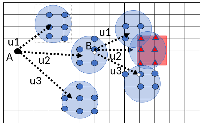
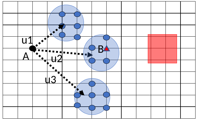
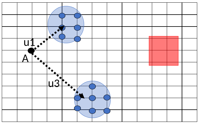
A graphical illustration of OCA is shown in Figure 2. The square denotes the obstacle and the intersections on the grid denote the states on the discrete state space . The triangle states are unsafe. The arrows show the state transitions given the control input, which is the FR procedure. Starting from Figure 2(a), the one-step forward reachability sets of state under all the control inputs, , and , have intersections with the obstacle, and hence these are unsafe control inputs and removed from state . Since there is no more (safe) control input left for state , i.e., , it is labeled as unsafe as in Figure 2(b). Since state is unsafe, control input is removed from state . This gives Figure 2(c), where state is safe with control inputs and , and state is in the sets and .
Inter-robot collision avoidance (Algorithm 4). Procedure ICA adopts a prioritized planning scheme [43] in each iteration and aims to further remove the control inputs that lead to collision with the robots with higher priority. Each robot is assigned with a unique priority level. The robots with higher priority are treated as moving obstacles and removes all the control inputs that lead to these obstacles. First, each robot broadcasts its reachability sets within an iteration at the beginning of each iteration . Upon receiving the messages from each robot with higher priority, i.e., , robot identifies a new set of unsafe states induced by in the discrete state space . Second, robot invokes procedure UnsafeUpdate to remove all the control inputs leading to the newly identified unsafe states. Robot then updates the set of the safe states by removing the new unsafe states . For each state , and any control can ensure collision avoidance with the obstacles and the robots with higher priority for one iteration. Notice that in the worst case, each robot removes all the control inputs in its own state-control space. Therefore, the worst-case computation complexity is independent of the number of robots.
III-C Active learning and real-time control (Algorithm 5)
In this section, we utilize the safe control inputs obtained above and synthesize a model predictive controller (MPC) to actively learn the disturbance and approach the goal.
First, the current state of robot is projected onto ; the projection is . Second, we capture the objective of goal reaching using distance , where is the discrete horizon of the MPC formulated below. Then the objective of exploration is described by a utility function ; candidate utility functions, e.g., , are available in [44]. Next, the safety constraint is honored by choosing control inputs from the safe control set . Lastly, the dynamic constraint is approximated by the one-step forward set . Formally, the controller returns control inputs by solving the finite-horizon optimal control problem:
| (3) |
where the decision variables are , subject to for all . To ensure the robot eventually reaches the goal, we select the weight for some such that diminishes.
The above finite-horizon optimal control problem is solved once for every time duration , and the returned control input is fixed for a duration . Specifically, consider a sequence , where , and . Procedure solves the above finite-horizon optimal control problem at . The solution has the form , and is returned as the control input, and for all , we have . The controller execution is denoted as procedure Execute in Algorithm 1.
III-D Performance guarantees
In this section, we provide the performance guarantees for dSLAP. To obtain theoretic guarantees, we assume that is a realization of a known Gaussian process. For notational simplicity, we assume . Generalizing to multi-dimensional can be done by applying the union bound.
Assumption III.1.
(Realization of process). It satisfies that and .
That is, function is a realization of Gaussian process with prior mean and kernel . This assumption is common in the analysis of GPR (Theorem 1, [45]). Theorem III.2 below provides the probability of the robots being safe until the end of an iteration if they are around the set of safe states at the beginning of the iteration.
Theorem III.2.
Denote . Then Theorem III.3 below provides the probability as well as the requirement on discretization and the computation speed of the robots such that they can be safe throughout the entire mission.
Theorem III.3.
The requirement for indicates that the robots’ onboard computation should be fast with respect to the speed of robots, while the computation can be relieved with coarse discretization. This provides the required update frequency for the decoupled controller.
The sufficient condition imposes a requirement in designing set-valued dynamics to discretize robot dynamics (1) using . Given Assumption III.1, represents an upper bound over the variability of the disturbances the robots want to tolerate. On the right hand side, represents the minimal spatial resolution. Then the sufficient condition implies that the product between the variability of the disturbances and the temporal resolution should be small with respect to and the spatial resolution.
III-E Discussion
(Probabilistic safety). The probability of the safety guarantees stems from the analysis of GPR estimates being able to capture the ground truth dynamics over the whole state-control space (and over all the iterations). The analysis can be conservative but is independent of the other components in the proposed algorithm. In order to reduce the probability of unsafe execution, or increase the probability of safe execution, the robots can increase according to the theorems. This may cause conservative actions as is a factor for constructing the one-step forward set and could lead to no solution at all if is too large. However, this can be addressed by having the robots collecting more data online to train the GPR such that becomes small.
(Verification of ). To ensure the robots are safe for all the time, Theorem III.3 implies that it suffices to satisfy the sufficient condition a priori. To achieve this, one can compute using data collected a priori or a prior conservative estimates of the disturbances. This prior knowledge can be obtained in most situations by, e.g., using historical data. Examples include wind speed, water current, and road texture in a local area. In addition, smaller can enlarge the set such that more initial states can satisfy the condition.
(Computation complexity). The algorithms in [37][38] aim for solving optimal arrival and collision avoidance simultaneously in a centralized manner. The computation complexities scale as , which grows exponentially in the number of robots. In order to reduce the computational complexity, dSLAP has two stages. The first stage includes procedure OCA and ICA, which are distributed and remove unsafe control inputs on the discrete state-control space of each robot. OCA is independent of the other robots. ICA augments the reachability sets of higher priority robots and correspondly removes the unsafe control inputs. Its worst-case onboard computational complexity of each robot scales linearly with . The local safe control inputs enable decoupled planning through AL in the second stage, whose computation complexity is also independent of . Furthermore, the computation complexity can be reduced during the implementation by successively removing the unsafe state-control pairs. Each state-control pair only needs to be removed at most once, and in each robot there are at most pairs to be removed, which is independent of .
(Strength and weakness). The proposed framework dSLAP is able to compute safe control inputs for a multi-robot system with general nonlinear dynamics in a distributed manner amid online uncertainty learning. Nevertheless, dSLAP can be conservative for the following two reasons. First, it overapproximates the continuous dynamics using discretized set-valued dynamics. To enable fast computation, the discretization is usually coarse and hence the approximation error can be large, which leads to conservative actions. However, this conservativeness can be reduced via finer discretization provided sufficient computation power. Second, the coordination among the robots is simple. The application of prioritized planning is suboptimal and can lose completeness [46]. Furthermore, higher priority robots are viewed as moving obstacles by lower priority robots. The overapproximation of the reachability sets in two iterations of the higher priority robots can be conservatives since the overapproximation is determined by the maximum speed of the robots multiplied by the duration of two iterations. This conservativeness can be reduced by developing a more sophisticated scheme of coordination among the robots, optimizing the assignment of priority levels, and/or shortening the duration of one iteration. We leave this for future work. Furthermore, dSLAP can suffer from the curse-of-dimensionality for each individual system.
IV Proof
In this section, we prove Theorems III.2 and III.3. Below is a roadmap for the proofs.
-
1.
We present the concentration inequality resulted from GPR in Section IV-A. This provides the probability of the event that belongs to the tube . The rest of the analysis is performed under this event.
- 2.
- 3.
-
4.
Given one-iteration safety in iteration , Section IV-D examines the distance between and as well as the inclusion of in terms of .
- 5.
IV-A Concentration inequality of Gaussian process
The concentration inequality resulted from GPR is presented in Lemma IV.1 below.
Lemma IV.1.
Under Assumption III.1, for any discretization parameter and each robot , the following holds with probability at least : ,
| (4) |
Proof: The proof mainly follows the proof of Lemma 5.1 in [45]. At iteration , we have the input dataset and output dataset , where
Let test input . Assumption III.1 gives
where , and
Applying identities of joint Gaussian distribution (page 200, [41]), we obtain the posterior distribution , where
Consider . It holds that for ,
where the inequality uses the fact for . Analogously, . Therefore, let and , we have . Denote event . Applying the union bound (Theorem 2-3, [47]), we have
Note that . Hence,
simultaneously for all with probability at least .
IV-B Set-valued approximation
In this section, we first introduce a set of set-valued notations from [38] to discretize system (1) in the time and state spaces. Lemma IV.2 shows that the set-valued discretization is a good approximation of the continuous system (1). Then we discuss other properties in the discrete space.
Define
Page 222 of [38] uses the following discrete set-valued map
| (5) |
which is discrete in time and state, to approximate system (1), which is continuous in time and state. Let
be the state at time when system (1) starts from at time and applies constant input within the time interval . Lemma IV.2 below shows that contains the trajectory of system (1) under constant control for any duration .
Lemma IV.2.
Under Assumption II.1, for any , , and , it holds that .
Similarly, let
| (7) |
Denote . By Lemma IV.1, we have
| (8) |
for all and with probability at least . This gives each of the followings holds with probability at least for all :
Lemma IV.3 characterizes the relation between and FR.
Lemma IV.3.
For any and , it holds that .
Proof: Consider state . Then
Hence This gives
where the right hand side is equivalent to .
Recall that Assumption II.1 implies that the system dynamics , or , is Lipschitz continuous. In particular, is identical to the example in the Lipschitz case on page 191 in [38], and hence it satisfies Assumptions H0, H1, and H2 in [38]. Therefore, applying Lemma 4.13 [38] gives
| (9) |
Below are the other properties in the discrete space. Lemmas IV.4 and IV.5 show that almost contains the union of .
Lemma IV.4.
Lemma IV.5.
Proof: We prove the claim by contradiction. Suppose (10) is true but there exists , such that .
Since is closed, there exists such that . Let be the -th element of . Define operation that finds the largest integer no greater than and recall . Denote real values and . Then for each dimension , we have two cases:
1). . Notice that . Choose . It is easy to see that .
2). . We can select if ; otherwise, we have , and we can select . Note that . Therefore under this selection, we have .
Let and . By definition, we can write
| (11) |
where . Let . Lemma IV.6 below characterizes the relation between and .
Lemma IV.6.
Suppose and (8) holds. It holds that .
Proof: Let . Denote . Then applying triangular inequality, we have
| (12) |
Next we find the upper bound of each term on the right hand side of (IV.6). Since , we have
| (13) |
Since , Lipschitz continuity yields . Then applying triangular inequality gives
| (14) |
Since (8) holds for all and , we have
| (15) |
Since , the Lipschitz continuity of renders . Then applying triangular inequality gives
Combining the above inequality with (14) gives
| (16) |
Applying triangular inequality, we can further write
| (17) |
where the last inequality follows from (IV.6).
IV-C Proof of Theorem III.2
Denote the obstacle regions (i.e., static obstacles and the robots with higher priority) for robot from time to . Denote shorthand for the state in discrete time.
Roadmap of the proof: First, in Lemma IV.7, we establish that is invariant in under inputs in . Then we examine the distance between and in Lemma IV.8. Next Lemma IV.10 utilizes the previous two lemmas to show that system (1) stays safe throughout for a duration under constant control, and Lemma IV.11 extends the safety result to the piecewise constant control law rendered by dSLAP for one iteration. Finally, we incorporate the concentration inequality in Lemma IV.1 and prove Theorem III.2.
Lemma IV.7.
For all , it holds that and for all .
Proof: We prove the lemma by contradiction.
Suppose . Control input removal only takes place in the OCA procedure and the UnsafeUpdate procedure. In both procedures, when it reduces to , the procedures rule that or , , through the Add procedure. Therefore, .
Suppose there exists , such that . Note that the OCA procedure constructs the set such that for all . Due to the UnsafeUpdate procedure, if and , we must have . Hence, this case is impossible.
The following lemma characterizes the distance between and .
Lemma IV.8.
It holds that for all .
Proof: Let . In OCA, when , is executed such that . Since ,
| (19) |
In ICA, when , . Therefore, by definition of , if
we must have . Hence
| (20) |
Recall that, for all iterations , AL and controller execution render , , as control inputs, each executed for a duration by robot such that for all . Then we have . The following lemma gives the sufficient conditions such that the robots are near the safe states within one iteration.
Lemma IV.9.
Proof: We prove the lemma using induction. For the base case , the condition in the lemma statement and the definition indicate that .
The following lemma characterizes a sufficient condition for the trajectory of system (1) under constant control input in to be safe for a duration .
Lemma IV.10.
Suppose Assumption II.1 holds and (8) is true , . If for all and some , it holds that
for all , and .
Proof: Recall that Lemma IV.3 implies for all and . Since , Lemma IV.7 renders . Thus, . Combining these with Lemma IV.8 gives
| (23) |
for all .
Lemma IV.2 gives . Since , we have . Combining these two statements and (23) with Lemma IV.5 renders
| (24) |
Then by the definition of , we have for all Combining this with (IV.10), it renders that, for all ,
Combining this with the definition of renders that
| (25) |
Note that (IV.10) holds for all , it further gives
By definitions, for any ,
Combining the above two statements completes the proof.
The following lemma gives the sufficient conditions such that the robots steered by dSLAP are safe within one iteration.
Lemma IV.11.
Now we are ready to prove Theorem III.2.
Proof of Theorem III.2: Given Assumptions II.1 and III.1 hold, for each robot , (8) holds with probability at least . Applying the union bound, this gives (8) holds with probability at least , , . Notice that Lemma IV.11 is given in the event of (8) is true , . Therefore, we have Lemma IV.11 hold with probability at least .
IV-D Proof of Theorem III.3
Recall that is the set of unsafe states induced by robot and is the set of unsafe states induced by static obstacles. Given Theorem III.2, we can prove Theorem III.3 by showing that if holds for iteration , it implies that also holds, and hence Theorem III.3 can be proved by induction. Therefore, under the condition of , we study: 1) the distance between and (Lemma IV.12); 2) the inclusion of in terms of (Lemma IV.14). The two results imply the distance between and and further characterize the conditions for (Lemma IV.16). Then the proof is concluded by combining these results.
D.1) The distance between and
Lemma IV.12.
Proof: Lemma IV.9 shows that there exists for each , . Therefore, by Lemma IV.7, for all control inputs , we have Based on OCA and ICA, we have
| (26) |
It implies that for all . By Discrete, this renders
for each . Combining this with Lemma IV.3, we have, for each ,
| (27) |
By Lemma IV.2, we have, for each ,
| (28) |
By definition of , we have, for each ,
| (29) |
Combining (27), (28) and (29) with Lemma IV.5, we have
for each . Recall that the definition that , and . Hence, the lemma is proved.
D.2) The inclusion of
Denote and . Then in ICA, we have and . Lemma IV.13 below renders a monotonic property.
Lemma IV.13.
It holds that .
Proof: Let . Equation (11) in [42] shows that can be expressed recursively as
where . Hence, and . Then the definition of yields .
The following lemma characterizes the inclusion of in terms of .
Lemma IV.14.
Proof: Consider . Let . By definition in OCA, it holds that and . Since Discrete renders , there exists satisfying . Then by triangular inequality, it holds that . This implies and hence . Since , we further have .
Consider . Let . By definition in ICA, it holds that . Since Discrete renders , we have . Recall that Lemma IV.13 renders . Since , it holds that . Combining the above three statements renders
This implies Similar to the logic above, Discrete renders that there exists satisfying . Triangular inequality further renders , or
and hence . Since , we have .
D.3) Conditions for
Define a sequence of sets such that , , and . Lemma IV.15 below characterizes using .
Lemma IV.15.
Suppose Assumption II.1 holds. For all iterations , it holds that for some . Furthermore, it holds that for all and for all .
Proof: By definition of , if , then
Therefore, we have for all . The definition indicates that and are mutually disjoint for any . Hence is finite since is finite due to the compactness of in Assumption II.1, and , and .
Now we show . For , according to the UnsafeUpdate procedure, we have . For any in non-empty , , since for all control inputs , it renders that , and hence according to UnsafeUpdate. Therefore, we have for all non-empty , . This shows .
We show using contradiction. Suppose there exists a state and for all , .
Obviously, we have because otherwise according to the definition of , . Then can only be added to by UnsafeUpdate. Then there exists such that , which reduces the control set to an empty set and leads to the addition of to . Furthermore, we also have for any since otherwise we have . By induction, we have a set but for any . However, this is impossible because is finite and . This gives .
The following lemma shows that the robot after one iteration is near the safe states under the priority assignment in the previous iteration.
Lemma IV.16.
Suppose Assumption II.1 holds. Suppose and (8) holds for all , , . Suppose . For each , if , , then .
Proof: Let Lemma IV.12 shows that . By (26), this implies that . Let . Then Lemma IV.7 renders that there exists such that . By Discrete and (26), this implies that, for all ,
| (30) |
Based on the UnsafeUpdate procedure, it is obvious that . Then (30) renders
| (31) |
Consider the rewriting in (11) and recall that and . Then (31) implies
| (32) |
Due to the Discrete procedure, there exists such that and . Then combining (32) with Lemma IV.6 renders
| (33) |
Recall that Lemma IV.14 renders
| (34) |
Then combining (33) and (34) renders
| (35) |
Note that (35) holds for all . Then it follows that
| (36) |
Combining the claim below with (26) renders that . Combining this with concludes the proof.
Claim IV.16.1.
It holds that .
Proof of Claim IV.16.1: The proof of the claim is composed of three parts.
Part (i). We show that
| (37) |
Let . Since , by (26) and Discrete, it renders that . According to the construction of through UnsafeUpdate, it holds that . Combining the above two statements renders
| (38) |
Next we show that through two cases.
Case 1: . By construction of in OCA, it holds that if and only if . Combining this with (38) renders . Recall that . Since , triangular inequality further gives . Hence .
Case 2: . Recall the definitions of and above Lemma IV.13. By construction of in ICA, it holds that if and only if . Combining this with (38) renders
Since , we have . Recall that Lemma IV.13 renders . Then combining the above three statements renders
Since , it holds that . Combining the above two statements with triangular inequality renders
Since , triangular inequality further gives
Hence . The proof of Part (i) is concluded.
Part (ii). Consider a sequence of states and control inputs pairs , , where
We use induction to show that, for all ,
| (39a) | |||
| (39b) | |||
Now consider (39) holds until . By the definition of and recall the rewriting in (11), it holds that
Recall that Discrete renders . Therefore, it holds that , and for every , there exists satisfying . Lemma IV.6 renders . Combining the above two statements renders
Then it follows from the induction hypothesis that
and hence . Furthermore, it follows from Lemma IV.7 that there exists such that , which implies
Note that Discrete renders . Hence, we can set . Then following the same logic of (30) to (36) by replacing with , with , and with , we have
The induction is completed.
Part (iii). Recall the definition of . Next we use induction to show that
| (40) |
Consider the base case and all . By (37) and (39a), we have . By (39a), we have . Hence, we have . Since , we have . Following the same logic, it follows that for all . This renders .
D.4) Proof of Theorem III.3
Given (8) holds for all , , , Lemma IV.16 implies that if , for some , then it holds that for all . Then Lemma IV.11 implies that , , ; i.e., .
Note that (2) renders that and , and dSLAP renders that . Hence, the definition of above (8) implies , . Therefore, for each , for each , (8) holds for all , , with probability at least . Denote as the event of (8) being violated for some and/or at iteration by robot . Then we have . Applying the union bound (Theorem 2-3, [47]) renders that . Note that . Hence, we have (8) holds with probability at least . Further applying the union bound renders that (8) holds and with probability at least .
V Simulation
In this section, we conduct a set of Monte Carlo simulations to evaluate the performance of the dSLAP algorithm. The simulations are run in Python, Linux Ubuntu 18.04 on an Intel Xeon(R) Silver 4112 CPU, 2.60 GHz with 32 GB of RAM.
Simulation scenarios. We evaluate the dSLAP algorithm using Zermelo’s navigation problem [49] in a 2D space under the following scenario: A group of robots are initially placed evenly on the plane and switch their positions at the destinations. The robots are immediately retrieved once they reach the goals. This example is also used in [50] [51] to demonstrate complicated multi-robot coordination scenarios.
Dynamic models. Consider constant-speed boat robots with length meters (m) moving at speed meters/seconds (m/s). For each robot , let and be the and coordinates on a 2D plane, be the angle between the heading and the -axis, and be the steering angle. The state space is given by . External wind disturbance is applied at such that the system dynamics has the following form: , , . The control takes discrete values and the control space is .
Parameters. The kernel of GPR is configured as , which is 0.0025 times the RBF kernel in the sklearn library. The factor 0.0025 is selected such that the supremum of the predictive standard deviation is 0.05, or 10% of the robots’ speed. This can be selected based on the prior knowledge of the variability of the disturbance. Other parameters are selected as , , , , , , , , and , which are determined according to the desired learning confidence level and the computation capability of the robots. To prevent prolonged computation due to unnecessarily fine discretization, we set a maximum such that .
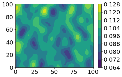
Random wind fields with different magnitudes. We randomly generate 2D spatial wind fields, with average speed in different ratios of the robots’ speed, i.e., , , and standard deviation 2% of the robots’ speed, using the Von Karman power spectral density function as described in [52]. This wind model is used to test multi-robot navigation in [52] [53]. A sample with is shown in Figure 4(a). We randomly generate 60 different wind fields for each .
V-A Safe grid vs. safe region
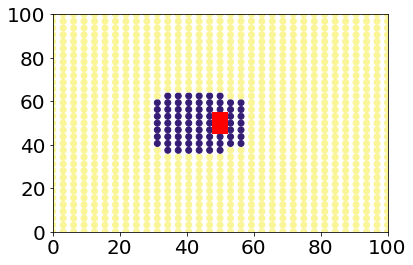
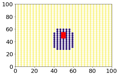
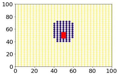
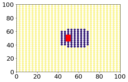
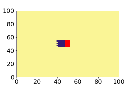
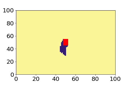
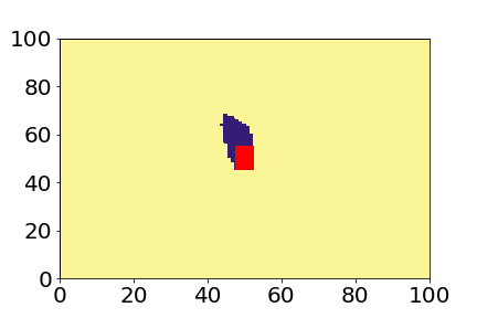
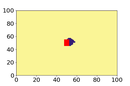
To visualize how safety is guaranteed by dSLAP, in this section, we compare the safe grids under the wind field in Figure 4(a) with the corresponding safe regions, which are the set of initial states that render safe arrival by applying the control policy returned. The comparison is similar for other wind fields. Since the dynamics of the robots has three dimensions, for simplicity of visualization, we only show the screen- shots of the 2D grids/regions with four different heading angles (i.e., and ). For the simplicity of illustration, we only compare the safe grids of robot , in the presence of only one obstacle, with the corresponding safe regions. Since the figures are similar for grids with different resolutions, due to space limitation, we only show the comparison for safe grids in one resolution, i.e., . In each figure, the safe region is approximated by 10,000 evenly distributed initial states.
Figure 3 shows the comparison for iteration , where the unsafe grids/regions are dark-colored and the safe grids/regions are light-colored. We can see that the safe grids are strictly subsets of the safe regions, which verifies the sufficient condition in Theorem III.2 and Theorem III.3, where the robots are guaranteed to be safe if . Furthermore, by comparing Figures 3(a) - 3(d) with Figures 3(e) - 3(h), we can see that the identification of safe grids by dSLAP and the safety guarantees by Theorem III.2 and Theorem III.3 are conservative. This is due to the fact that the safe control inputs are spatially similar, and hence some unsafe states labeled by dSLAP can still be safe by applying the control inputs on the nearest safe states. The conservativeness comes from the over-approximation of the one-step forward reachability sets in and the errors in discretization. Nevertheless, the conservativeness can be reduced by refining the discretization in the expense of more computation power.
V-B Multi-robot maneuver.
We evaluate the dSLAP algorithm using 30,000 scenarios generated as follows.
Different initial configurations. We deploy robots with 10 different initial configurations in the simulation, where . Figure 4(b) shows one configuration of 8 robots’ initial states and goal regions, and the corresponding trajectories under dSLAP in the wind field in Figure 4(a). The circular disks are the goal regions of the robots and the red rectangle is the static obstacle. Other configurations are generated by different permutations and removals of robots from that in Figure 4(b).

Ablation study. To the best of our knowledge, this paper is the first to consider multi-robot motion planning coupled with online learning. Hence, we compare dSLAP with its three variants, Vanilla, Robust and Known, that do not learn the wind disturbances. Vanilla assumes , , whereas Robust assumes and thus , where . We adopt such that Robust has the same level of conservativeness as dSLAP before collecting any data. The benchmark Known is obtained by running the dSLAP framework with the disturbances exactly known, which is the control law obtained by dSLAP when the amount of data of goes to infinity.
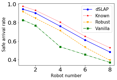
Results. The average safe arrival rates of dSLAP, Robust, Vanilla and Known among the 30,000 cases are shown in Figure 5. From Figure 5(a), we can see that dSLAP’s performance is superior to those of Robust and Vanilla. This is due to the fact that dSLAP online learns about the unknown disturbances and adjusts the policies accordingly. On the other hand, Robust (or Vanilla) only captures part of (or none of) the disturbances through the prior estimates, which can be unsafe when the disturbances exceed the estimates. Furthermore, we can observe that the safe arrival rate for dSLAP decreases linearly with respect to the number of robots. This corresponds to the probability with respect to the number of robots in Theorems III.2 and III.3. Notice that the gap between Known and dSLAP is small. The cases that are unsafe even in Known are due to the robots being too close to each other or the magnitude of the disturbances being too large to tolerate (note that the magnitude of the disturbances can be as large as the speed of the robots in the simulation). This indicates that dSLAP enables safe arrival in most feasible cases.
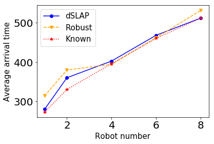
Arrival time. Figure 5(b) compares the average safe arrival times among dSLAP, Robust and Known. We exclude the comparison with Vanilla since its safe arrival rate is far lower than the other three while safety is this paper’s top priority. The arrival times of the three algorithms are comparable. This indicates dSLAP improves safe arrival rate without sacrificing arrival time, i.e., being more conservative.
| ID | Total time | SL | Discrete+OCA | ICA | AL | ||||
| time | Percentage | time | Percentage | time | Percentage | time | Percentage | ||
| 1 | 5.710.45 | 0.847.87 | 14.731.08 | 4.260.12 | 74.913.95 | 6.031.85 | 0.119.44 | 0.610.32 | 10.265.07 |
| 2 | 5.930.47 | 0.810.01 | 13.701.03 | 4.210.06 | 71.325.10 | 0.060.03 | 1.080.59 | 0.850.41 | 13.906.38 |
| 3 | 5.690.34 | 0.821.43 | 14.480.88 | 4.140.04 | 73.103.90 | 0.140.01 | 2.560.32 | 0.580.32 | 9.875.08 |
| 4 | 5.180.14 | 0.822.03 | 15.850.43 | 4.010.04 | 77.371.98 | 0.160.09 | 3.071.76 | 0.200.15 | 3.702.81 |
| 5 | 5.900.35 | 0.820.01 | 13.960.65 | 4.300.08 | 73.103.41 | 0.230.03 | 3.960.51 | 0.540.27 | 8.984.10 |
| 6 | 5.661.29 | 0.880.16 | 15.70.65 | 4.551.08 | 80.261.58 | 0.130.11 | 2.572.23 | 0.100.13 | 1.461.64 |
| 7 | 5.940.99 | 0.880.10 | 14.960.82 | 4.490.65 | 75.852.69 | 0.190.10 | 3.392.03 | 0.380.38 | 5.795.19 |
| 8 | 5.941.14 | 0.880.13 | 14.900.55 | 4.650.83 | 78.531.30 | 0.290.07 | 5.021.62 | 0.120.22 | 1.562.45 |
V-C Run-time computation.
This section shows the wall computation time of dSLAP when the robots are deployed in the wind field in Figure 4(a) with configuration in Figure 4(b), as an example. Table I presents the average plus/minus one standard deviation of each robot’s onboard computation time for one iteration for each component of dSLAP and the corresponding percentages (%) of the total computation time. Discrete+OCA consumes most of the computation resources because a discrete set-valued approximation of the continuous dynamics over the entire state-action space is constructed through these two procedures, especially in OCA. Table I shows that the computation costs of the other procedures are mostly sub-second. Table II shows that the average wall time plus/minus one standard deviation per iteration for each robot versus the number of robots deployed. This shows that the computation time within each robot is nearly independent of the number of robots.
V-D Hyperparameter tuning
The parameters in Algorithm 1, include mission and system parameters (, , , , and ) and tuned parameters: Kernel for GPR: ; Initial discretization parameter: ; Termination iteration: ; Number of samples to be obtained in each iteration: ; Discrete time unit: ; Time horizon for MPC: ; Weight in the MPC: ; Sampling period: ; Utility function . Below we provide an overall guidance on tuning these parameters. More detailed guidance can be found in Appendix A.
Parameters , , , , and , are referred as the computation parameters, since they are related to the computation power of the machine performing the simulation or the onboard computer of the robots. In the simulation, these parameters, though can affect performance, determine how much computation power is needed to compute the safe control inputs. Therefore, they can be mainly tuned based on how much computation power is available and how much computation time is desired in one iteration. The remaining parameters, referred as the learning parameters, to be tuned are: , , and . Notice that the above parameters are more related to the learning of the unknown dynamics using GPR and active learning. Therefore, standard/common parameters in the related literature are used in the simulation. They can be tuned by following the general guidance of hyperparameter tuning for GPR [41] and active learning [44].
| Number of robots | 1 | 2 | 4 | 6 | 8 |
| Wall time |
VI Conclusion and future work
We study the problem where a group of mobile robots subject to unknown external disturbances aim to safely reach goal regions. We propose the dSLAP algorithm that enables the robots to quickly adapt to a sequence of learned models resulted from online Gaussian process regression, and safely reach the goal regions. We provide sufficient conditions to ensure the safety of the system. The developed algorithm is evaluated by Monte Carlo simulation. Exciting future works can be done in the direction of considering sparse communication network, developing more sophisticated coordination scheme and/or optimizing the assignment of priority levels to reduce conservativeness in inter-robot collision avoidance.
References
- [1] S. M. LaValle, Planning algorithms. Cambridge university press, 2006.
- [2] L. Lindemann, M. Cleaveland, Y. Kantaros, and G. J. Pappas, “Robust motion planning in the presence of estimation uncertainty,” in Proc. IEEE Conf. Decision and Control (CDC), 2021, pp. 5205–5212.
- [3] M. H. Cohen, C. Belta, and R. Tron, “Robust control barrier functions for nonlinear control systems with uncertainty: A duality-based approach,” in Proc. IEEE Conf. Decision and Control (CDC), 2022, pp. 174–179.
- [4] A. Lakshmanan, A. Gahlawat, and N. Hovakimyan, “Safe feedback motion planning: A contraction theory and l 1-adaptive control based approach,” in Proc. IEEE Conf. Decision and Control (CDC), 2020, pp. 1578–1583.
- [5] M. Omainska, J. Yamauchi, T. Beckers, T. Hatanaka, S. Hirche, and M. Fujita, “Gaussian process-based visual pursuit control with unknown target motion learning in three dimensions,” SICE Journal of Control, Measurement, and System Integration, vol. 14, no. 1, pp. 116–127, 2021.
- [6] M. Ono, M. Pavone, Y. Kuwata, and J. Balaram, “Chance-constrained dynamic programming with application to risk-aware robotic space exploration,” Autonomous Robots, vol. 39, no. 4, pp. 555–571, 2015.
- [7] M. Castillo-Lopez, P. Ludivig, S. A. Sajadi-Alamdari, J. L. Sanchez-Lopez, M. A. Olivares-Mendez, and H. Voos, “A real-time approach for chance-constrained motion planning with dynamic obstacles,” IEEE Robotics and Automation Letters, vol. 5, no. 2, pp. 3620–3625, 2020.
- [8] N. Virani, D. K. Jha, Z. Yuan, I. Shekhawat, and A. Ray, “Imitation of demonstrations using bayesian filtering with nonparametric data-driven models,” Journal of Dynamic Systems, Measurement, and Control, vol. 140, no. 3, 2018.
- [9] S. Gupta, J. Davidson, S. Levine, R. Sukthankar, and J. Malik, “Cognitive mapping and planning for visual navigation,” in Proc. IEEE Conf. Computer Vision and Pattern Recognition (CVPR), 2017, pp. 2616–2625.
- [10] S. Levine, C. Finn, T. Darrell, and P. Abbeel, “End-to-end training of deep visuomotor policies,” The Journal of Machine Learning Research, vol. 17, pp. 1334–1373, 2016.
- [11] A. Majumdar and M. Goldstein, “PAC-Bayes control: Synthesizing controllers that provably generalize to novel environments,” in Conf. Robot Learning (CoRL), 2018, pp. 293–305.
- [12] J. F. Fisac, A. K. Akametalu, M. N. Zeilinger, S. Kaynama, J. Gillula, and C. J. Tomlin, “A general safety framework for learning-based control in uncertain robotic systems,” IEEE Trans. Automatic Control, vol. 64, no. 7, pp. 2737–2752, 2018.
- [13] K. P. Wabersich, L. Hewing, A. Carron, and M. N. Zeilinger, “Probabilistic model predictive safety certification for learning-based control,” IEEE Trans. Automatic Control, vol. 67, no. 1, pp. 176–188, 2021.
- [14] T. Koller, F. Berkenkamp, M. Turchetta, and A. Krause, “Learning-based model predictive control for safe exploration,” in Proc. IEEE Conf. Decision and Control (CDC), 2018, pp. 6059–6066.
- [15] K. P. Wabersich and M. N. Zeilinger, “Predictive control barrier functions: Enhanced safety mechanisms for learning-based control,” IEEE Trans. Automatic Control, vol. 68, no. 5, pp. 2638–2651, 2022.
- [16] R. Cosner, M. Tucker, A. Taylor, K. Li, T. Molnar, W. Ubelacker, A. Alan, G. Orosz, Y. Yue, and A. Ames, “Safety-aware preference-based learning for safety-critical control,” in Learning for Dynamics and Control Conference, 2022, pp. 1020–1033.
- [17] S. Curi, A. Lederer, S. Hirche, and A. Krause, “Safe reinforcement learning via confidence-based filters,” in Proc. IEEE Conf. Decision and Control (CDC), 2022, pp. 3409–3415.
- [18] N. Kochdumper, H. Krasowski, X. Wang, S. Bak, and M. Althoff, “Provably safe reinforcement learning via action projection using reachability analysis and polynomial zonotopes,” IEEE Open Journal of Control Systems, vol. 2, pp. 79–92, 2023.
- [19] Z. Zhou, O. S. Oguz, M. Leibold, and M. Buss, “A general framework to increase safety of learning algorithms for dynamical systems based on region of attraction estimation,” IEEE Trans. Robotics, vol. 36, no. 5, pp. 1472–1490, 2020.
- [20] J. H. Reif, “Complexity of the mover’s problem and generalizations,” in Annual Symposium on Foundations of Computer Science, 1979, pp. 421–427.
- [21] J. T. Schwartz and M. Sharir, “On the “piano movers” problem. ii. general techniques for computing topological properties of real algebraic manifolds,” Advances in Applied Mathematics, vol. 4, no. 3, pp. 298–351, 1983.
- [22] G. Zhao and M. Zhu, “Pareto optimal multirobot motion planning,” IEEE Trans. Automatic Control, vol. 66, no. 9, pp. 3984–3999, 2020.
- [23] D. V. Dimarogonas, S. G. Loizou, K. J. Kyriakopoulos, and M. M. Zavlanos, “A feedback stabilization and collision avoidance scheme for multiple independent non-point agents,” Automatica, vol. 42, no. 2, pp. 229–243, 2006.
- [24] D. V. Dimarogonas and K. J. Kyriakopoulos, “Connectedness preserving distributed swarm aggregation for multiple kinematic robots,” IEEE Trans. Robotics, vol. 24, no. 5, pp. 1213–1223, 2008.
- [25] L. Wang, A. D. Ames, and M. Egerstedt, “Safety barrier certificates for collisions-free multirobot systems,” IEEE Trans. Robotics, vol. 33, no. 3, pp. 661–674, 2017.
- [26] G. Zhao and M. Zhu, “Scalable distributed algorithms for multi-robot near-optimal motion planning,” Automatica, vol. 140, p. 110241, 2022.
- [27] K. E. Bekris, D. K. Grady, M. Moll, and L. E. Kavraki, “Safe distributed motion coordination for second-order systems with different planning cycles,” The International Journal of Robotics Research, vol. 31, no. 2, pp. 129–150, 2012.
- [28] X. Ma, Z. Jiao, Z. Wang, and D. Panagou, “3-d decentralized prioritized motion planning and coordination for high-density operations of micro aerial vehicles,” IEEE Trans. Control Systems Technology, vol. 26, no. 3, pp. 939–953, 2017.
- [29] J. Van Den Berg, P. Abbeel, and K. Goldberg, “LQG-MP: Optimized path planning for robots with motion uncertainty and imperfect state information,” The International Journal of Robotics Research, vol. 30, no. 7, pp. 895–913, 2011.
- [30] T. Pan, C. K. Verginis, A. M. Wells, L. E. Kavraki, and D. V. Dimarogonas, “Augmenting control policies with motion planning for robust and safe multi-robot navigation,” in Proc. IEEE/RSJ Int. Conf. Intelligent Robots and Systems (IROS), 2020, pp. 6975–6981.
- [31] Y. Zhou, H. Hu, Y. Liu, S.-W. Lin, and Z. Ding, “A distributed approach to robust control of multi-robot systems,” Automatica, vol. 98, pp. 1–13, 2018.
- [32] A. D. Saravanos, A. Tsolovikos, E. Bakolas, and E. A. Theodorou, “Distributed covariance steering with consensus admm for stochastic multi-agent systems.” in Robotics: Science and Systems, 2021.
- [33] H. Zhu, B. Brito, and J. Alonso-Mora, “Decentralized probabilistic multi-robot collision avoidance using buffered uncertainty-aware voronoi cells,” Autonomous Robots, vol. 46, no. 2, pp. 401–420, 2022.
- [34] R. Cheng, M. J. Khojasteh, A. D. Ames, and J. W. Burdick, “Safe multi-agent interaction through robust control barrier functions with learned uncertainties,” in Proc. IEEE Conf. Decision and Control (CDC), 2020, pp. 777–783.
- [35] P. Long, T. Fanl, X. Liao, W. Liu, H. Zhang, and J. Pan, “Towards optimally decentralized multi-robot collision avoidance via deep reinforcement learning,” in Proc. Int. Conf. Robotics and Automation (ICRA), 2018, pp. 6252–6259.
- [36] T. Fan, P. Long, W. Liu, and J. Pan, “Distributed multi-robot collision avoidance via deep reinforcement learning for navigation in complex scenarios,” The International Journal of Robotics Research, vol. 39, no. 7, pp. 856–892, 2020.
- [37] G. Zhao and M. Zhu, “Pareto optimal multi-robot motion planning,” IEEE Trans. Automatic Control, vol. 66, no. 9, pp. 3984–3999, 2021.
- [38] P. Cardaliaguet, M. Quincampoix, and P. Saint-Pierre, “Set-valued numerical analysis for optimal control and differential games,” in Stochastic and differential games. Springer, 1999, pp. 177–247.
- [39] Z. Yuan and M. Zhu, “dSLAP: Distributed safe learning and planning for multi-robot systems,” in Proc. IEEE Conf. Decision and Control (CDC), 2022, pp. 5864–5869.
- [40] C. K. Batchelor and G. Batchelor, An introduction to fluid dynamics. Cambridge university press, 2000.
- [41] C. K. Williams and C. E. Rasmussen, Gaussian Processes for Machine Learning. MIT Press, 2006.
- [42] M. F. Huber, “Recursive Gaussian process: On-line regression and learning,” Pattern Recognition Letters, vol. 45, pp. 85–91, Aug. 2014.
- [43] M. Erdmann and T. Lozano-Perez, “On multiple moving objects,” Algorithmica, vol. 2, no. 1-4, p. 477, 1987.
- [44] B. Settles, “Active learning literature survey,” University of Wisconsin-Madison Department of Computer Sciences, Tech. Rep., 2009.
- [45] N. Srinivas, A. Krause, S. M. Kakade, and M. W. Seeger, “Information-theoretic regret bounds for Gaussian process optimization in the bandit setting,” IEEE Trans. Information Theory, vol. 58, no. 5, pp. 3250–3265, Jan. 2012.
- [46] H. Ma, D. Harabor, P. J. Stuckey, J. Li, and S. Koenig, “Searching with consistent prioritization for multi-agent path finding,” in Proceedings of the AAAI conference on artificial intelligence, vol. 33, no. 01, 2019, pp. 7643–7650.
- [47] A. Papoulis and S. U. Pillai, Probability, Random Variables, and Stochastic Processes. New Delhi, India: Tata McGraw-Hill Education, 2002.
- [48] S. Boyd and L. Vandenberghe, Convex Optimization. Cambridge university press, 2004.
- [49] S. Zlobec, Zermelo’s Navigation Problems. Boston, MA: Springer US, 2001.
- [50] H. G. Tanner and A. Boddu, “Multiagent navigation functions revisited,” IEEE Trans. Robotics, vol. 28, no. 6, pp. 1346–1359, 2012.
- [51] O. Arslan, D. P. Guralnik, and D. E. Koditschek, “Coordinated robot navigation via hierarchical clustering,” IEEE Trans. Robotics, vol. 32, no. 2, pp. 352–371, 2016.
- [52] K. Cole and A. Wickenheiser, “Impact of wind disturbances on vehicle station keeping and trajectory following,” in AIAA Guidance, Navigation, and Control Conference, 2013, p. 4865.
- [53] K. Cole and A. M. Wickenheiser, “Reactive trajectory generation for multiple vehicles in unknown environments with wind disturbances,” IEEE Trans. Robotics, vol. 34, no. 5, pp. 1333–1348, 2018.
![[Uncaptioned image]](/html/2207.07824/assets/figures/Zhenyuan_Yuan.jpg) |
Zhenyuan Yuan is a Ph.D. candidate in the School of Electrical Engineering and Computer Science at the Pennsylvania State University. He received B.S. in Electrical Engineering and B.S. in Mathematics from the Pennsylvania State University in 2018. His research interests lie in machine learning and motion planning with applications in robotic networks. He is a recipient of the Rudolf Kalman Best Paper Award of the ASME Journal of Dynamic Systems Measurement and Control in 2019 and the Penn State Alumni Association Scholarship for Penn State Alumni in the Graduate School in 2021. |
![[Uncaptioned image]](/html/2207.07824/assets/figures/Minghui-ZHU.jpg) |
Minghui Zhu is an Associate Professor in the School of Electrical Engineering and Computer Science at the Pennsylvania State University. Prior to joining Penn State in 2013, he was a postdoctoral associate in the Laboratory for Information and Decision Systems at the Massachusetts Institute of Technology. He received Ph.D. in Engineering Science (Mechanical Engineering) from the University of California, San Diego in 2011. His research interests lie in distributed control and decision-making of multi-agent networks with applications in robotic networks, security and the smart grid. He is the co-author of the book ”Distributed optimization-based control of multi-agent networks in complex environments” (Springer, 2015). He is a recipient of the Dorothy Quiggle Career Development Professorship in Engineering at Penn State in 2013, the award of Outstanding Reviewer of Automatica in 2013 and 2014, and the National Science Foundation CAREER award in 2019. He is an associate editor of the IEEE Open Journal of Control Systems, the IET Cyber-systems and Robotics and the Conference Editorial Board of the IEEE Control Systems Society. |
Appendix A Hyperparameter tuning
Regarding the tuning of the parameters, there are actually not too many parameters to be freely tuned for the sake of performance. As in Algorithm 1, the parameters, other than those related to the mission or the systems (i.e., State space: , Control input space: , Obstacle: , Goal: , Lipschitz constant , Prior supremum of dynamic model ), needed to be tuned are: Kernel for GPR: ; Initial discretization parameter: ; Termination iteration: ; Number of samples to be obtained: ; Discrete time unit: ; Time horizon for MPC: ; Weight in the MPC: ; Sampling period: ; Utility function . Below we provide the guidance on tuning the parameters.
Computation parameters:
-
•
Initial discretization parameter : The larger the discretization parameter, while provides tighter approximation of the one-step forward reachability sets, the more computation is needed to build up the graph of one-step forward reachability set.
-
•
Termination iteration : The larger termination iteration, the longer the simulation would run if neither arrival nor collision happens before.
-
•
Number of samples to be obtained : While the larger the number of samples to be obtained in each iteration generally provide better learning results of the unknown dynamics, it also requires longer time to recursively train the GP model.
-
•
Discrete time unit : The larger the discrete time unit, the long each iteration would last, which can make the safe planning in ICA more conservative. Therefore, each iteration should stop right after all the modules (i.e., SL, Discrete, OCA, ICA and AL)) in Fig. 1 are done computing.
-
•
Time horizon for MPC : The larger the time horizon for MPC, while improves the optimality of the solution, the more computation power is needed.
Learning parameters:
-
•
Kernel for GPR : In the simulation, we use a square-exponential kernel, which is one of the most common kernels used in GPR-related applications [41].
-
•
Sampling period : This parameter is related to how to sample each robot’s trajectory in each iteration to obtain data for training the GPR. With larger sampling period, the collected data would be more spatially separated over the trajectories of the robots. In the simulation, is chosen such that the data are temporally uniformly distributed over the trajectories of the robots.
-
•
Utility function : This determines provide guidance to the robots on where they should go to collect new data. In the simulation, we use predictive variance as the utility function, which is one of the most common utility function in active learning [44].
-
•
Weight in the MPC : The parameter determines the weights between the utility function for active learning and the distance-to-goal for arrival. It is rather not important as eventually as more weight is eventually put on distance-to-goal, according to the definition of . With higher , the robots would explore for more iteration, which could lead to a better learned model of the unknown dynamics.