Model order reduction for parameterized electromagnetic problems using matrix decomposition and deep neural networks

Abstract

A non-intrusive model order reduction (MOR) method for solving parameterized electromagnetic scattering problems is proposed in this paper. A database collecting snapshots of high-fidelity solutions is built by solving the parameterized time-domain Maxwell equations for some values of the material parameters using a fullwave solver based on a high order discontinuous Galerkin time-domain (DGTD) method. To perform a prior dimensionality reduction, a set of reduced basis (RB) functions are extracted from the database via a two-step proper orthogonal decomposition (POD) method. Projection coefficients of the reduced basis functions are further compressed through a convolutional autoencoder (CAE) network. Singular value decomposition (SVD) is then used to extract the principal components of the reduced-order matrices generated by CAE, and a cubic spline interpolation-based (CSI) approach is employed for approximating the dominating time- and parameter-modes of the reduced-order matrices. The generation of the reduced basis and the training of the CAE and CSI are accomplished in the offline stage, thus the RB solution for given time/parameter values can be quickly recovered via outputs of the interpolation model and decoder network. In particular, the offline and online stages of the proposed RB method are completely decoupled, which ensures the validity of the method. The performance of the proposed CAE-CSI ROM is illustrated with numerical experiments for scattering of a plane wave by a 2-D dielectric disk and a multi-layer heterogeneous medium.

Key words: non-intrusive reduced-order modeling; parameterized electromagnetic scattering; proper orthogonal decomposition; convolutional autoencoder; cubic spline interpolation

1 Introduction

Electromagnetic wave interaction with heterogeneous media is generally modeled by the system of parameterized time-domain Maxwell equations [22]. The Finite Difference Time-Domain (FDTD) method [46, 39, 10] is the most popular method for simulating these time-domain electromagnetic wave propagation problems. The discontinuous Galerkin time-domain (DGTD) method is an alternative approach that has emerged during the last 20 years [20, 8]. Compared with the FDTD method, the DGTD method has several attractive advantages such as local approximation strategy, easy adaption to complex geometry and material composition [20]. With the DGTD method, the number of degree of freedom (DOFs) is determined by the underlying mesh and the polynomial order used for approximating the EM field components. This number is usually high to guarantee the accuracy of the solution of Maxwell’s equations. Therefore, it makes sense to study the model order reduction method to reduce the computational burden of CPU time and memory, when repeatedly simulating Maxwell’s equations with different parameters. Model order reduction (MOR) techniques [3] aim to replace a full-order model (FOM) by a reduced-order model (ROM), featuring a much lower dimension, thereby reducing computational cost under acceptable accuracy conditions. A reduced basis (RB) method based on a offline-online procedure is a widely used model order reduction technique [18, 14, 30, 41]. During the offline stage, a reduced space spanned by a set of time- and parameter-independent RB functions is constructed from the full-order solutions (snapshots), which are for instance generated by the DGTD method at different parameter values. The reduced-order solution for a new time and parameter value can be expressed as a linear combination of the RB functions where the combination coefficients, also called the intrinsic coordinates, need to be calculated during the online stage. The high-fidelity solver is only used to generate the snapshots, thus guaranteeing a complete decoupling between the online evaluation and the offline training [44, 30].

More recently, non-intrusive ROM combining RB techniques and machine learning have been developed for solving large-scale complex physical problems. The advantage of these methods is that they are data-driven and do not require access to the governing equations of the original FOM. For instance, a non-intrusive RB method combining POD and feed forward neural networks (FNNs) has been proposed for parameterized unsteady flows [19, 41], where a neural network is trained to approximate the mapping between the time/parameter values and the projection coefficients. Moreover, different regression and interpolation methods such as Gaussian process regression (GPR) [13, 14, 48, 23], radial basis functions (RBF) [43, 27] and cubic spline interpolation (CSI) [30, 4, 35] have also been considered in place of FNNs to approximate the mapping from the time/parameter to the reduced coefficients. By combining an ANN-based regression model with a physics-informed neural network (PINN) [37, 31], a hybrid strategy is devised in [5] to train a network by minimizing the residual loss of the reduced-order equation at a set of points in the parameter space.

However, linear reduction methods such as POD hardly capture the complex dynamics of highly nonlinear systems, therefore nonlinear manifold learning methods such as Kernel PCA [49] and Hessian feature maps [45] have attracted much attention in the past several years. Assuming that data points lie in a low dimensional manifold embedded in an higher dimensional Euclidean space, manifold learning [32] aims to identify the intrinsic dimensionality, equal to the number of parameters that describe the system, and thus obtain low dimensional representations of the data points. Although kernel PCA and Hessian feature maps are effective in providing low dimensional representations for high dimensional data points, their main drawback is that they do not provide an analytical formula to decode the compressed data back to their high dimensional representation in the original space [34]. An autoencoder (AE) overcomes this disadvantage by learning how to compress (encode) a high dimensional data to a low dimensional code and then reconstruct (decode) the code to a representation as close to the original input as possible [34]. The encoder and decoder parts of an autoencoder are trained simultaneously but can be used separately, which provides an opportunity to build a mapping between the input time/parameter and encoded representation.

Directly applying large-scale simulation data (snapshots) to a fully-connected autoencoder is not only computationally prohibitive, but also ignores the opportunity to exploit the structure of features in high dimensional data [12, 9]. As an extension of ordinary autoencoders, convolutional autoencoders (CAEs) [25, 15] are characterized by shared parameters and local connectivity which help to reduce the memory as well as computational costs. For example, projection-based ROMs proposed in [26] project dynamic systems onto nonlinear manifolds by means of autoencoders, which still require the assembling and solution of a ROM as in traditional POD-Galerkin ROMs. In [12], a reduced trial manifold is generated via a deep convolutional recurrent AE, which is then used to train a long short-term memory (LSTM) network that models the reduced dynamics. A POD-DL-ROM approach proposed in [9] combines and improves the previous two methods as the nonlinear trial manifold is learnt by using the decoder function of a CAE while the dynamics on the reduced manifold is modeled through a DFNN and the encoder function of a CAE. In [34], the authors utilize a CAE in conjunction with a FNN to establish a mapping from the problem’s parametric space to its solution space. The differences between [9] and [34] are that the former uses the POD method for pre-dimensionality reduction to reduce training time and trains CAE and FNN at the same time.

In this paper, a non-intrusive reduced-order modeling strategy is proposed to solve electromagnetic scattering problems governed by parameterized time-domain Maxwell equations. Firstly, the approach performs a prior dimensionality reduction by a two-step POD method [30]. Then, relying on its powerful dimensionality reduction properties, we use a CAE to encode and decode the intrinsic coordinates. Furthermore, a CSI-based model is devised to approximate a mapping from the problem’s parameter space to its low dimensional encoded vector space. Using this approach, the encoded representation of the solution at a new time/parameter value is recovered by the CSI model, while the RB solution in the original high dimensional space is obtained by the decoder and projection matrix. The resulting CAE-CSI ROM provides a very fast and accurate evaluation of the entire system response.

The paper is organized as follows. In section 2, we briefly introduce the time-domain Maxwell equations and the DGTD scheme to generate the snapshots. Section 3 provides a description for the two-step POD, from which a RB basis is constructed. In section 4, we present how a CAE is employed to further reduce the dimension of intrinsic coordinates. In section 5, we show how to use CSI to build an approximate mapping between the problem’s parameters and the low dimensional encoded vectors. The overall CAE-CSI ROM for parameterized electromagnetic scattering problems is also presented in this section. In Section 6, two numerical experiments for testing the method are provided. And conclusion remarks are drawn in section 7.

2 Full-order model and DGTD method

Unsteady electromagnetic scattering problems are governed by the following normalized form of the time-domain Maxwell equations

$$\begin{cases}\nu_{r}\dfrac{\partial\mathbf{H}(\mathbf{x},t)}{\partial t}+\operatorname{curl}(\mathbf{E}(\mathbf{x},t))=0,&\forall(\mathbf{x},t)\in\Omega\times\mathcal{T},\\ \varepsilon_{r}\dfrac{\partial\mathbf{E}(\mathbf{x},t)}{\partial t}-\operatorname{curl}(\mathbf{H}(\mathbf{x},t))=0,&\forall(\mathbf{x},t)\in\Omega\times\mathcal{T},\\ \mathcal{L}(\mathbf{E}(\mathbf{x},t),\mathbf{H}(\mathbf{x},t))=\mathcal{L}\left(\mathbf{E}^{\text{inc }}(\mathbf{x},t),\mathbf{H}^{\text{inc }}(\mathbf{x},t)\right),&\forall(\mathbf{x},t)\in\partial\Omega\times\mathcal{T},\\ \mathbf{E}(\mathbf{x},0)=\mathbf{E}_{0}(\mathbf{x}),\mathbf{H}(\mathbf{x},0)=\mathbf{H}_{0}(\mathbf{x}),&\forall\mathbf{x}\in\Omega,\end{cases}$$ (1)

where $\Omega$ is the spatial domain and $\mathcal{T}=\left[0,T_{f}\right)$ is the time interval, $\mathbf{E}=\left(E_{x},E_{y},E_{z}\right)^{T}$ and $\mathbf{H}=\left(H_{x},H_{y},H_{z}\right)^{T}$ are the electric field and the magnetic field respectively, $\varepsilon_{r}$ and $\nu_{r}$ denote the relative electric permittivity and magnetic permeability parameters respectively. In this work we consider the first-order Silver-Müller absorbing boundary condition $(\mathrm{ABC})$ [33]

$$\mathcal{L}(\mathbf{E}(\mathbf{x},t),\mathbf{H}(\mathbf{x},t))=\mathbf{n}\times\mathbf{E}(\mathbf{x},t)+Z\mathbf{n}\times(\mathbf{n}\times\mathbf{H}(\mathbf{x},t)),\text{ on }\partial\Omega,$$ (2)

where $\partial\Omega$ is the boundary of $\Omega$, $\mathbf{n}$ denotes the outer unit normal vector along $\partial\Omega$, $\mathbf{E}^{\rm{inc}}$ and $\mathbf{H}^{\rm{inc}}$ are the incident fields, and $Z=\sqrt{\nu_{r}/{\varepsilon_{r}}}$. Our goal is to solve equation (1) with varying parameter $\varepsilon_{r}\in\mathcal{P}$, where $\mathcal{P}$ denotes the parameter domain.

System (1) is discretized in space by means of discontinuous Galerkin method, and in time by means of a second-order leapfrog scheme. The time interval $\mathcal{T}=\left[0,T_{f}\right)$ is divided into $m$ equal subintervals as $0=t_{0}<$ $t_{1}<\cdots<t_{m}=T_{f}$ with $t_{n}=n\Delta t\left(n=0,1,\cdots,m\right)$, and $\Delta t$ denotes the time step size. The fully discrete scheme of DGTD based on centered fluxes and second-order Leap-Frog time stepping [8] is given by

$$\left\{\begin{array}[]{l}\mathbb{M}^{\varepsilon_{r}}\dfrac{\underline{\mathbf{E}}_{h}\left(t_{n+1}\right)-\underline{\mathbf{E}}_{h}\left(t_{n}\right)}{\Delta t}=\left(\mathbb{K}-\mathbb{S}^{i}\right)\underline{\mathbf{H}}_{h}(t_{n+\frac{1}{2}})-\mathbb{S}^{h}\underline{\mathbf{H}}_{h}(t_{n+\frac{1}{2}})-\mathbf{B}^{h}(n\Delta t),\\[7.11317pt] \mathbb{M}^{\nu_{r}}\dfrac{\underline{\mathbf{H}}_{h}(t_{n+\frac{3}{2}})-\underline{\mathbf{H}}_{h}(t_{n+\frac{1}{2}})}{\Delta t}=\left(-\mathbb{K}+\mathbb{S}^{i}\right)\underline{\mathbf{E}}_{h}(t_{n+1})+\mathbb{S}^{e}\widehat{\mathbf{E}}_{h}(t_{n+1})+\mathbf{B}^{e}((n+\frac{1}{2})\Delta t).\end{array}\right.$$ (3)

Here $\mathbb{M}^{\varepsilon_{r}}$ and $\mathbb{M}^{\nu_{r}}$ are the mass matrices, $\mathbb{K}$ is the stiffness matrix, $\mathbb{S}^{i}$ is the surface matrix for the interior faces, and $\mathbb{S}^{h}$ and $\mathbb{S}^{e}$ are the boundary face matrices. For more detailed definition of these matrices we refer to [40, 29].

3 Two-step POD method

3.1 Snapshot-based data collection

For the parameterized time-dependent problem, let $\mathcal{P}_{h}^{tr}=\{\boldsymbol{\mu}_{1},\boldsymbol{\mu}_{2},\cdots,\boldsymbol{\mu}_{\mathcal{N}_{p}}\}$ be a parameter sampling over the parameter domain $\mathcal{P}$. A collection of high-fidelity solutions can be obtained by solving system (1) with the DGTD solver for different parameter values $\boldsymbol{\mu}\in\mathcal{P}_{h}^{tr}$ in a time sampling $\mathcal{T}_{h}=\{t_{1},t_{2},\cdots,t_{m}\}$. Then we uniformly select $\mathcal{N}_{t}$ transient solutions in $\mathcal{T}_{h}^{tr}=\{t_{n_{1}},t_{n_{2}},\cdots,t_{n_{\mathcal{N}_{t}}}\}\subseteq\mathcal{T}_{h}$ to form the time trajectory matrix $\mathbf{S}_{\mathbf{u}}^{j}\in\mathbb{R}^{\mathcal{N}_{h}\times\mathcal{N}_{t}}$, which takes the form

$$\mathbf{S}_{\mathbf{u}}^{j}=\left(\begin{array}[]{cccc}\mathbf{u}_{h,1}\left(t_{n_{1}},\boldsymbol{\mu}_{j}\right)&\mathbf{u}_{h,1}\left(t_{n_{2}},\boldsymbol{\mu}_{j}\right)&\cdots&\mathbf{u}_{h,1}(t_{n_{\mathcal{N}_{t}}},\boldsymbol{\mu}_{j})\\ \mathbf{u}_{h,2}\left(t_{n_{1}},\boldsymbol{\mu}_{j}\right)&\mathbf{u}_{h,2}\left(t_{n_{2}},\boldsymbol{\mu}_{j}\right)&\cdots&\mathbf{u}_{h,2}(t_{n_{\mathcal{N}_{t}}},\boldsymbol{\mu}_{j})\\ \vdots&\vdots&\ddots&\vdots\\ \mathbf{u}_{h,\mathcal{N}_{h}}\left(t_{n_{1}},\boldsymbol{\mu}_{j}\right)&\mathbf{u}_{h,\mathcal{N}_{h}}\left(t_{n_{2}},\boldsymbol{\mu}_{j}\right)&\cdots&\mathbf{u}_{h,\mathcal{N}_{h}}(t_{n_{\mathcal{N}_{t}}},\boldsymbol{\mu}_{j})\end{array}\right)\text{with}\ j=1,2,\cdots,\mathcal{N}_{p},\mathbf{u}\in\{\mathbf{E},\mathbf{H}\},$$ (4)

and the snapshot matrix for all parameters in $\mathcal{P}_{h}^{tr}$ is

$$\mathbf{S}_{\mathbf{u}}=\left[\mathbf{S}_{\mathbf{u}}^{1}\ |\ \mathbf{S}_{\mathbf{u}}^{2}\ |\ \cdots\ |\ \mathbf{S}_{\mathbf{u}}^{\mathcal{N}_{p}}\right]\in\mathbb{R}^{\mathcal{N}_{h}\times\mathcal{N}_{s}},\mathbf{u}\in\{\mathbf{E},\mathbf{H}\},$$ (5)

where $\mathcal{N}_{s}=\mathcal{N}_{t}\cdot\mathcal{N}_{p}$, $\mathbf{u}_{h}(t,\boldsymbol{\mu})\in\mathbb{R}^{\mathcal{N}_{h}}$ is the high-fidelity solution, and $\mathcal{N}_{h}$ is the number of DOFs, which is determined by the underlying mesh and polynomial order of the discretization scheme.

Directly reducing the dimensionality of the snapshots through a neural network will result in an overwhelming computational burden when the FOM dimension $\mathcal{N}_{h}$ becomes moderately large. The CAE-CSI technique proposed here can be considered as a non-intrusive ROM technique in which a three-step dimensionality reduction is performed. First, a two-step POD strategy is applied on a set of FOM snapshots. Then a convolutional autoencoder is utilized to reduce the dimensionality of the projection coefficients (also called intrinsic coordinates) generated by POD. Lastly, a CSI-based model is built to approximate the mapping between input parameters $(t,\boldsymbol{\mu})$ and the reduced-order matrices.

3.2 Two-step POD for dimensionality reduction

In this subsection, we perform a low-rank approximation to the snapshot matrix $\mathbf{S}_{\mathbf{u}}$ and construct a low dimensional space $\mathcal{V}_{\mathbf{u},rb}$ with dimension $\mathcal{N}\ll\operatorname{min}\{\mathcal{N}_{h},\mathcal{N}_{s}\}$. Spanned by a group of time- and parameter-independent RB functions, the reduced space is expressed as

$$\mathcal{V}_{\mathbf{u},rb}=\operatorname{span}\left\{\mathbf{v}_{\mathbf{u},1},\mathbf{v}_{\mathbf{u},2},\cdots,\mathbf{v}_{\mathbf{u},\mathcal{N}}\right\},\mathbf{u}\in\{\mathbf{E},\mathbf{H}\}.$$ (6)

The POD method is a popular technique to compress data and extract an optimal set of RB functions in the least-squares sense. The POD basis of size $\mathcal{N}$ is the solution to the minimization problem

$$\min_{\mathbf{V_{u}}\in\mathbb{R}^{\mathcal{N}_{h}\times\mathcal{N}}}\left\|\mathbf{S_{u}}-\mathbf{V_{u}}\mathbf{V}_{\mathbf{u}}^{T}\mathbf{S_{u}}\right\|_{F},$$ (7)

$$\text{ s.t. }\quad\mathbf{V}_{\mathbf{u}}^{T}\mathbf{V_{u}}=\mathbf{I},$$

where $\|\cdot\|_{F}$ is the Frobenius norm and $\mathbf{I}\in\mathbb{R}^{\mathcal{N}\times\mathcal{N}}$ is an identity matrix.

According to the Eckart-Young theorem [38, 7], the solution of $(\ref{eq:pod_ls})$ is given by the first $\mathcal{N}$ left singular vectors of the matrix $\mathbf{S_{u}}$, which can be obtained through the singular value decomposition (SVD)

$$\mathbf{W}_{\mathbf{u}}^{T}\mathbf{S}_{\mathbf{u}}\mathbf{Z}_{\mathbf{u}}=\left(\begin{array}[]{cc}\Sigma_{r_{\mathbf{u}}\times r_{\mathbf{u}}}^{\mathbf{u}}&\mathbf{O}_{r_{\mathbf{u}}\times\left(\mathcal{N}_{s}-r_{\mathbf{u}}\right)}\\ \mathbf{O}_{\left(\mathcal{N}_{h}-r_{\mathbf{u}}\right)\times r_{\mathbf{u}}}&\mathbf{O}_{\left(\mathcal{N}_{h}-r_{\mathbf{u}}\right)\times\left(\mathcal{N}_{s}-r_{\mathbf{u}}\right)}\end{array}\right)=\mathbf{D}_{\mathbf{u}},\mathbf{u}\in\{\mathbf{E},\mathbf{H}\},$$ (8)

where $\mathbf{W}_{\mathbf{u}}=[\mathbf{w}_{\mathbf{u},1},\mathbf{w}_{\mathbf{u},2},\cdots,\mathbf{w}_{\mathbf{u},\mathcal{N}_{h}}]$ and $\mathbf{Z}_{\mathbf{u}}=[\mathbf{z}_{\mathbf{u},1},\mathbf{z}_{\mathbf{u},2},\cdots,\mathbf{z}_{\mathbf{u},\mathcal{N}_{s}}]$ are $\mathcal{N}_{h}\times\mathcal{N}_{h}$ and $\mathcal{N}_{s}\times\mathcal{N}_{s}$ orthogonal matrices respectively, and $\sum_{r_{\mathbf{u}}\times r_{\mathbf{u}}}^{\mathbf{u}}=\operatorname{diag}\left(\sigma_{\mathbf{u},1},\sigma_{\mathbf{u},2},\cdots,\sigma_{\mathbf{u},r_{\mathbf{u}}}\right)$. The singular values $\sigma_{\mathbf{u},1}\geq\sigma_{\mathbf{u},2}\geq\cdots\geq\sigma_{\mathbf{u},r_{\mathbf{u}}}\geq 0$ of $\mathbf{S}_{\mathbf{u}}$ are sorted in descending order, and $r_{\mathbf{u}}$ is the rank of $\mathbf{S}_{\mathbf{u}}$. The POD basis with $\mathcal{N}\left(\mathcal{N}\ll r_{\mathbf{u}}\right)$ vectors is the set $\left\{\mathbf{v}_{\mathbf{u},i}\right\}_{i=1}^{\mathcal{N}}$ with $\mathbf{v}_{\mathbf{u},i}=\mathbf{w}_{\mathbf{u},i}$, which can minimize the projection error of the snapshots among all $\mathcal{N}$-dimensional orthogonal basis in $\mathbb{R}^{\mathcal{N}_{h}}$. The error bound can be evaluated using the singular values

$$\sum_{i=1}^{\mathcal{N}_{s}}\left\|\mathbf{S}_{\mathbf{u}}(:,i)-\mathbf{V_{u}}\mathbf{V}_{\mathbf{u}}^{T}\mathbf{S}_{\mathbf{u}}(:,i)\right\|_{\mathbb{R}^{\mathcal{N}_{h}}}^{2}=\sum_{j=\mathcal{N}+1}^{r_{\mathbf{u}}}\sigma_{\mathbf{u},j}^{2},$$ (9)

where $\mathbf{V}_{\mathbf{u}}=\left[\mathbf{v}_{\mathbf{u},1},\cdots,\mathbf{v}_{\mathbf{u},\mathcal{N}}\right]$, $\mathbf{u}\in\{\mathbf{E},\mathbf{H}\}$. According to (9), it is clear that the error in the POD basis is equal to the sum of the squares of the neglected singular values, i.e., the error can be controlled by $\mathcal{N}$. In this work, POD is utilized to perform a moderate dimensionality reduction of the snapshots data, thus yielding a linear subspace of dimension $\mathcal{N}\ll\mathcal{N}_{h}$.

However, since $\mathcal{N}_{s}=\mathcal{N}_{t}\cdot\mathcal{N}_{p}$ is large, performing SVD on such a large-scale snapshot matrix directly is extremely expensive. We adopt a two-step POD method to effectively save the computational cost. The detailed process is as follow and also shown in Algorithm 1:

1. For each time trajectory matrix $\mathbf{S}_{\mathbf{u}}^{j}$, $j=$ $1,2,\cdots,\mathcal{N}_{p}$, the POD basis $\{\gamma_{\mathbf{u},i}^{j}\}_{i=1}^{k}$ are obtained through SVD, then assemble them to a matrix $\mathbf{T}_{\mathbf{u}}^{j}=[\gamma_{\mathbf{u},1}^{j},\gamma_{\mathbf{u},2}^{j},\cdots,\gamma_{\mathbf{u},k}^{j}]$;

2. Assemble a composite matrix $\mathbf{T}_{\mathbf{u}}=[\mathbf{T}_{\mathbf{u}}^{1}\ |\ \mathbf{T}_{\mathbf{u}}^{2}\ |\ \cdots\ |\ \mathbf{T}_{\mathbf{u}}^{\mathcal{N}_{p}}]$ with the matrices generated in the first step, then perform POD on $\mathbf{T}_{\mathbf{u}}$ with truncation $\mathcal{N}$. The POD basis $\{\mathbf{v}_{\mathbf{u},i}\}_{i=1}^{\mathcal{N}}$ is obtained, i.e., $\mathbf{V}_{\mathbf{u}}=[\mathbf{v}_{\mathbf{u},1},\cdots,\mathbf{v}_{\mathbf{u},\mathcal{N}}]$.

According to the projection theory [28], one can obtain the reduced-order solution and the projection coefficients or intrinsic coordinates as

$$\left\{\begin{array}[]{l}\mathbf{u}_{h}^{r}(t,\boldsymbol{\mu})=\mathbf{V}_{\mathbf{u}}\left(\mathbf{V}_{\mathbf{u}}^{T}\mathbf{V}_{\mathbf{u}}\right)^{-1}\mathbf{V}_{\mathbf{u}}^{T}\mathbf{u}_{h}(t,\boldsymbol{\mu})=\mathbf{V}_{\mathbf{u}}\mathbf{V}_{\mathbf{u}}^{T}\mathbf{u}_{h}(t,\boldsymbol{\mu}),\\[7.11317pt] \alpha_{\mathbf{u}}(t,\boldsymbol{\mu})\equiv\mathbf{u}_{\mathcal{N}}(t,\boldsymbol{\mu})=\left(\mathbf{V}_{\mathbf{u}}^{T}\mathbf{V}_{\mathbf{u}}\right)^{-1}\mathbf{V}_{\mathbf{u}}^{T}\mathbf{u}_{h}(t,\boldsymbol{\mu})=\mathbf{V}_{\mathbf{u}}^{T}\mathbf{u}_{h}(t,\boldsymbol{\mu}),\end{array}\mathbf{u}\in\{\mathbf{E},\mathbf{H}\}.\right.$$ (10)

Thus, the reduced-order solution $\mathbf{u}_{h}^{r}(t,\boldsymbol{\mu})$ serves as an approximation to the high-fidelity solution $\mathbf{u}_{h}(t,\boldsymbol{\mu})$ and can be represented as

$$\mathbf{u}_{h}^{r}(t,\boldsymbol{\mu})=\mathbf{V_{u}}\alpha_{\mathbf{u}}(t,\boldsymbol{\mu})=\sum_{i=1}^{\mathcal{N}}\alpha_{\mathbf{u},i}(t,\boldsymbol{\mu})\mathbf{v}_{\mathbf{u},i},\mathbf{u}\in\{\mathbf{E},\mathbf{H}\},$$ (11)

where $\alpha_{\mathbf{u}}(t,\boldsymbol{\mu})=\left[\alpha_{\mathbf{u},1}(t,\boldsymbol{\mu}),\alpha_{\mathbf{u},2}(t,\boldsymbol{\mu}),\cdots,\alpha_{\mathbf{u},\mathcal{N}}(t,\boldsymbol{\mu})\right]^{T}\in\mathbb{R}^{\mathcal{N}}$ collects the combination coefficients.

In our previous work [48, 30] we constructed the mapping between the time/parameter values and the projection coefficients by decoupling time- and parameters-modes through SVD. However, these ROMs need to create too many regression or interpolation models. The approach we proposed here firstly reduces the length of projection coefficients $\alpha_{\mathbf{u}}(t,\boldsymbol{\mu})$ or intrinsic coordinates $\mathbf{u}_{\mathcal{N}}(t,\boldsymbol{\mu})$ from $\mathcal{N}$ to a fairly small $n$ through a convolutional autoencoder, then constructs the mapping between the time/parameter values and the low-dimensional coded representation using cubic spline interpolation, thus reducing the number of interpolation models as well as test time online.

1

Input : Time trajectory matrices $\mathbf{S}_{\mathbf{u}}^{j}\left(j=1,2,\cdots,\mathcal{N}_{p},\mathbf{u}\in\{\mathbf{E},\mathbf{H}\}\right)$, truncation parameter $k$ and size parameter $\mathcal{N}$

Output : POD basis matrix $\mathbf{V}_{\mathbf{u}}\ (\mathbf{u}\in\{\mathbf{E},\mathbf{H}\})$

2 Compute the compressed matrices $\mathbf{T}_{\mathbf{u}}^{j}=$POD $(\mathbf{S}_{\mathbf{u}}^{j},k)$ for $j=1,2,\cdots,\mathcal{N}_{p},\mathbf{u}\in\{\mathbf{E},\mathbf{H}\}$;

3 Assemble the matrix $\mathbf{T}_{\mathbf{u}}=[\mathbf{T}_{\mathbf{u}}^{1}\ |\ \mathbf{T}_{\mathbf{u}}^{2}\ |\ \cdots\ |\ \mathbf{T}_{\mathbf{u}}^{\mathcal{N}_{p}}]\ (\mathbf{u}\in\{\mathbf{E},\mathbf{H}\})$ for all parameter values;

4 Calculate the POD basis matrix $\mathbf{V}_{\mathbf{u}}=$POD $\left(\mathbf{T}_{\mathbf{u}},\mathcal{N}\right)\ (\mathbf{u}\in\{\mathbf{E},\mathbf{H}\})$ Function $\mathbf{V}=$ POD $(\mathbf{A},k)$

5       Perform $\operatorname{eig}(\mathbf{A}^{T}\mathbf{A})$ in MATLAB, and get the eigenvalues $\lambda_{1}\geq\lambda_{2}\geq\cdots\geq\lambda_{r}>0$ and the corresponding orthogonal eigenvectors $\mathbf{u}_{1},\mathbf{u}_{2},\cdots,\mathbf{u}_{r}$ with $r$ being the rank of $\mathbf{A}$;

6       Compute the POD basis functions $\mathbf{v}_{i}=\dfrac{1}{\sqrt{\lambda_{i}}}\mathbf{A}\mathbf{u}_{i},i=1,2,\cdots,k,k\ll r$;

7       Obtain the POD basis matrix $\mathbf{V}=[\mathbf{v}_{1},\mathbf{v}_{2},\cdots,\mathbf{v}_{k}]$.

8 end

Algorithm 1 Two-step POD method

Remark 1.

According to (9), the error bounds in the first and second steps of the two-step POD algorithm are written as

$$\left\{\begin{array}[]{l}\sum\limits_{i=1}^{\mathcal{N}_{t}}\left\|\mathbf{S}_{\mathbf{u}}^{j}(:,i)-\mathbf{T}_{\mathbf{u}}^{j}(\mathbf{T}_{\mathbf{u}}^{j})^{T}\mathbf{S}_{\mathbf{u}}^{j}(:,i)\right\|_{\mathbb{R}^{\mathcal{N}_{h}}}^{2}=\sum\limits_{i=k+1}^{r_{\mathbf{u}}^{j}}(\sigma_{\mathbf{u},i}^{j})^{2},1\leqslant j\leqslant\mathcal{N}_{p},\\ \sum\limits_{j=1}^{\mathcal{N}_{p}}\sum\limits_{i=1}^{k}\left\|\mathbf{T}_{\mathbf{u}}^{j}(:,i)-\mathbf{V}_{\mathbf{u}}\mathbf{V}_{\mathbf{u}}^{T}\mathbf{T}_{\mathbf{u}}^{j}(:,i)\right\|_{\mathbb{R}^{\mathcal{N}_{h}}}^{2}=\sum\limits_{i=\mathcal{N}+1}^{r_{\mathbf{u}}}\left(\sigma_{\mathbf{u},i}\right)^{2},\end{array}\right.$$ (12)

where $r_{\mathbf{u}}$ and $r_{\mathbf{u}}^{j}\ \left(j=1,2,\cdots,\mathcal{N}_{p},\mathbf{u}\in\{\mathbf{E},\mathbf{H}\}\right)$ are the rank of $\mathbf{S}_{\mathbf{u}}$ and $\mathbf{S}_{\mathbf{u}}^{j}$, and $\left\{\sigma_{\mathbf{u},i}\right\}_{i=1}^{r_{\mathbf{u}}}$ as well as $\{\sigma_{\mathbf{u},i}^{j}\}_{i=1}^{r_{\mathbf{u}}^{j}}$ are the corresponding singular values. The two-step POD projection error can be bounded as

$$\sum_{j=1}^{\mathcal{N}_{p}}\sum_{i=1}^{\mathcal{N}_{t}}\left\|\mathbf{S}_{\mathbf{u}}^{j}(:,i)-\mathbf{V}_{\mathbf{u}}\mathbf{V}_{\mathbf{u}}^{T}\mathbf{S}_{\mathbf{u}}^{j}(:,i)\right\|_{\mathbb{R}^{\mathcal{N}_{h}}} \leqslant\sum_{j=1}^{\mathcal{N}_{p}}\sum_{i=1}^{\mathcal{N}_{t}}\left\|\mathbf{S}_{\mathbf{u}}^{j}(:,i)-\mathbf{T}_{\mathbf{u}}^{j}(\mathbf{T}_{\mathbf{u}}^{j})^{T}\mathbf{S}_{\mathbf{u}}^{j}(:,i)\right\|_{\mathbb{R}^{\mathcal{N}_{h}}}$$

$$+\sum_{j=1}^{\mathcal{N}_{p}}\sum_{i=1}^{\mathcal{N}_{t}}\left\|\mathbf{T}_{\mathbf{u}}^{j}(\mathbf{T}_{\mathbf{u}}^{j})^{T}\mathbf{S}_{\mathbf{u}}^{j}(:,i)-\mathbf{V}_{\mathbf{u}}\mathbf{V}_{\mathbf{u}}^{T}\mathbf{T}_{\mathbf{u}}^{j}(\mathbf{T}_{\mathbf{u}}^{j})^{T}\mathbf{S}_{\mathbf{u}}^{j}(:,i)\right\|_{\mathbb{R}^{\mathcal{N}_{h}}}$$

$$+\sum_{j=1}^{\mathcal{N}_{p}}\sum_{i=1}^{\mathcal{N}_{t}}\left\|\mathbf{V}_{\mathbf{u}}\mathbf{V}_{\mathbf{u}}^{T}\mathbf{T}_{\mathbf{u}}^{j}(\mathbf{T}_{\mathbf{u}}^{j})^{T}\mathbf{S}_{\mathbf{u}}^{j}(:,i)-\mathbf{V}_{\mathbf{u}}\mathbf{V}_{\mathbf{u}}^{T}\mathbf{S}_{\mathbf{u}}^{j}(:,i)\right\|_{\mathbb{R}^{\mathcal{N}_{h}}}$$

$$\leqslant\mathcal{L}_{1}+\mathcal{L}_{2},\mathbf{u}\in\{\mathbf{E},\mathbf{H}\},$$

where

$$\left\{\begin{array}[]{l}\mathcal{L}_{1}=(1+\left\|\mathbf{V}_{\mathbf{u}}\mathbf{V}_{\mathbf{u}}^{T}\right\|_{F})\sum\limits_{j=1}^{\mathcal{N}_{p}}(\mathcal{N}_{t}\sum\limits_{i=k+1}^{r_{\mathbf{u}}^{j}}(\sigma_{\mathbf{u},i}^{j})^{2})^{\frac{1}{2}},\\ \mathcal{L}_{2}=\max\limits_{1\leqslant j\leqslant\mathcal{N}_{p}}\sum\limits_{i=1}^{\mathcal{N}_{t}}\|\mathbf{S}_{\mathbf{u}}^{j}(:,i)\|_{\mathbb{R}^{\mathcal{N}_{h}}}\max\limits_{\begin{subarray}{c}1\leqslant i\leqslant k\\ 1\leqslant j\leqslant\mathcal{N}_{p}\end{subarray}}\|\mathbf{T}_{\mathbf{u}}^{j}(:,i)\|_{\mathbb{R}^{\mathcal{N}_{h}}}(k\mathcal{N}_{p}\sum\limits_{i=\mathcal{N}+1}^{r_{\mathbf{u}}}(\sigma_{\mathbf{u},i})^{2})^{\frac{1}{2}}.\end{array}\right.$$

Therefore, the accuracy of the two-step POD can be controlled by the truncation parameter $k$ and size parameter $\mathcal{N}$.

4 Convolutional autoencoders for model reduction

In this section, we present an approach to construct a nonlinear manifold, which compresses the dimensionality of projection coefficients $\alpha_{\mathbf{u}}(t,\boldsymbol{\mu})\equiv\mathbf{u}_{\mathcal{N}}(t,\boldsymbol{\mu})\in\mathbb{R}^{\mathcal{N}}$ $(\mathbf{u}\in\{\mathbf{E},\mathbf{H}\})$ from $\mathcal{N}$ to a fairly small $n$. In data-driven sciences, the manifold hypothesis presumes that real-world high dimensional data lie near a low dimensional manifold $\mathcal{S}$ embedded in $\mathbb{R}^{m}$, where $m$ is large [2]. As a result POD has been widely used for dimensionality reduction of physical systems. However the main drawback is that POD can only construct an optimal linear manifold while data sampled from complex real-world systems tends to be strongly nonlinear.

A nonlinear generalization of POD is the autoencoder, which takes the the form of a fully-connected neural network shown in Fig. 1. Specifically, an autoencoder includes two parts: the encoder maps a high dimensional input to a low-dimensional latent vector, known as encoding; then the decoder learns how to reconstruct the original input from the latent vector with a minimum error.

Figure 1: Network architecture of a fully-connected autoencoder.

A basic autoencoder consists of a single or multiple layer encoder network

$$\mathbf{h}=f_{E}\left(\mathbf{x};\boldsymbol{\theta}_{E}\right),$$ (13)

where $\boldsymbol{\theta}_{E}$ denotes the weights and the biases of the encoder network, $\mathbf{x}\in\mathbb{R}^{\mathcal{N}}$ is the input state, $\mathbf{h}\in\mathbb{R}^{n}$ is the feature or low dimensional representation vector with $n\ll\mathcal{N}$. A decoder network is then used to reconstruct $\mathbf{x}$ by

$$\hat{\mathbf{x}}=f_{D}\left(\mathbf{h};\boldsymbol{\theta}_{D}\right).$$ (14)

The objective is how to train this autoencoder and find the parameters that minimize the mean squared error over all training examples

$$\boldsymbol{\theta}_{E}^{*},\boldsymbol{\theta}_{D}^{*}=\mathop{\arg\min}\limits_{\boldsymbol{\theta}_{E},\boldsymbol{\theta}_{D}}\|\mathbf{x}-\hat{\mathbf{x}}\|^{2}.$$ (15)

Note that directly applying large-scale snapshots to fully connected autoencoders is not only computationally expensive, but also ignores opportunities to exploit feature structures in high dimensional data. So we adopt an convolutional autoencoder which is characterized by shared parameters and local connectivity, thus reduce the memory as well as computational cost.

4.1 Basics of convolutional and deconvolutional layers

Some basic operations in convolutional and transposed convolutional layers are introduced in this subsection. The reader is referred to [6, 47] for more details of the convolution operations.

For simplicity, we consider a 3-D tensor $\mathcal{X}\in\mathbb{R}^{c\times h\times w}$ as an input of the convolutional neural network, with $c$, $h$ and $w$ being the number of channels, height and width respectively. The convolution operations aim to extract the most important features from the input $\mathcal{X}$ and then use them to construct a feature map $\mathcal{G}$. Specifically, the output at the $(l-1)$th layer is $\mathcal{X}^{l-1}\in\mathbb{R}^{c_{q}^{l-1}\times h^{l-1}\times w^{l-1}}$, and the feature map at $l$th layer is denoted as a tensor $\mathcal{G}^{l}\in\mathbb{R}^{c_{p}^{l}\times n_{1}^{l}\times n_{2}^{l}}$ with $c_{p}^{l}=c_{q}^{l-1}$ and element $\mathcal{G}_{i,j,k}^{l}$ representing a unit within channel $i$ at row $j$ and column $k$. The filter banks collecting a set of kernels at $l$th layer can be considered as a 4-dimensional tensor $\mathcal{W}^{l}\in\mathbb{R}^{c_{p}^{l}\times c_{q}^{l}\times k_{h}^{l}\times k_{w}^{l}}$ with element $\mathcal{W}_{i,j,m,n}^{l}$ connecting between a unit in channel $i$ of the output and a unit in channel $j$ of the input, with an offset of $m$ rows and $n$ columns between the output unit and the input unit. $c_{p}$ denotes the number of kernels in the filter bank, and the kernel size is denoted by $k_{h}$ and $k_{w}$. Convolution between a feature map $\mathcal{G}^{l-1}$ and a filter bank $\mathcal{W}^{l}$ can be expressed as

$$\mathcal{G}_{i,j,k}^{l}=\sigma_{l}\left(\sum_{r,m,n}\mathcal{G}_{r,(j-1)\times s+m,(k-1)\times s+n}^{l-1}\mathcal{W}_{i,r,m,n}^{l}+\mathcal{B}_{i,j,k}^{l}\right),$$ (16)

where $\sigma_{l}$ is a nonlinear activation function and $\mathcal{B}^{l}$ is a bias. Here, $s$ denotes the stride, which determines the downsampling rate of each convolution. The dimension of the next feature map can be reduced by a factor $s$ in each direction when $s>1$. The kernel size $[k_{h},k_{w}]$, the number of filters $c_{p}$ and the stride $s$ are the hyperparameters while the filter banks $\mathcal{W}$ and the biases $\mathcal{B}$ are learnable parameters. A deconvolutional layer performs the reverse operations of convolution, called transposed convolution, and it is used to construct decoding layers [26]. In summary, the architecture of CAE shown in Fig. 2 is composed of convolutional, deconvolutional and dense layers, which is used for dimensionality reduction and reconstruction.

4.2 Data preparation

In this subsection, we present a procedure to generate a data set for training. Provided the high-fidelity snapshots and the orthogonal basis $\mathbf{V_{u}}\in\mathbb{R}^{{\mathcal{N}_{h}}\times\mathcal{N}}$ ($\mathbf{u}\in\{\mathbf{E},\mathbf{H}\}$) generated by the two-step POD method, we compute the projection coefficients or intrinsic coordinates $\alpha_{\mathbf{u}}(t,\boldsymbol{\mu})=\mathbf{u}_{\mathcal{N}}(t,\boldsymbol{\mu})=\mathbf{V}_{\mathbf{u}}^{T}\mathbf{u}_{h}(t,\boldsymbol{\mu})$ ($\mathbf{u}\in\{\mathbf{E},\mathbf{H}\}$) to perform a moderate dimensionality reduction, and the projection coefficient matrix $\mathbf{C_{u}}$ takes the form

$$\mathbf{C}_{\mathbf{u}}=\left[\mathbf{C}_{\mathbf{u}}^{1}\ |\ \mathbf{C}_{\mathbf{u}}^{2}\ |\ \cdots\ |\ \mathbf{C}_{\mathbf{u}}^{\mathcal{N}_{p}}\right]\in\mathbb{R}^{\mathcal{N}\times\mathcal{N}_{s}},\ \mathbf{u}\in\{\mathbf{H},\mathbf{E}\},$$ (17)

where $\mathbf{C}_{\mathbf{u}}^{j}=\mathbf{V}_{\mathbf{u}}^{T}\mathbf{S}_{\mathbf{u}}^{j}\in\mathbb{R}^{\mathcal{N}\times\mathcal{N}_{t}}$, $j=1,2,\cdots\mathcal{N}_{p}$. Next, we randomly shuffle $\mathbf{C_{u}}$ by column and split it into training set and validation set according to a training-validation splitting fraction $\lambda$, i.e., $\mathbf{C_{u}}=[\mathbf{C}_{\mathbf{u}}^{\rm{tr}},\mathbf{C}_{\mathbf{u}}^{\rm{val}}]$, $\mathbf{u}\in\{\mathbf{H},\mathbf{E}\}$, where $\mathbf{C}_{\mathbf{u}}^{\rm{tr}}\in\mathbb{R}^{\mathcal{N}\times\lambda\mathcal{N}_{s}}$. As the training speed of neural network is affected by the range of input/output [21], feature scaling is required before feeding the training data into the network. The input data $\mathbf{C}_{\mathbf{u}}^{\rm{tr}}$ and $\mathbf{C}_{\mathbf{u}}^{\rm{val}}$ are normalized to $[0,1]$ through the following affine transformation

$$\mathbf{C}_{\mathbf{u}}^{\rm{tr}}(i,j)=\frac{\mathbf{C}_{\mathbf{u}}^{\rm{tr}}(i,j)-\mathop{\min}\limits_{1\leqslant i\leqslant\mathcal{N}}\mathop{\min}\limits_{1\leqslant j\leqslant\lambda\mathcal{N}_{s}}\mathbf{C}_{\mathbf{u}}^{\rm{tr}}(i,j)}{\mathop{\max}\limits_{1\leqslant i\leqslant\mathcal{N}}\mathop{\max}\limits_{1\leqslant j\leqslant\lambda\mathcal{N}_{s}}\mathbf{C}_{\mathbf{u}}^{\rm{tr}}(i,j)-\mathop{\min}\limits_{1\leqslant i\leqslant\mathcal{N}}\mathop{\min}\limits_{1\leqslant j\leqslant\lambda\mathcal{N}_{s}}\mathbf{C}_{\mathbf{u}}^{\rm{tr}}(i,j)}.$$ (18)

We then reshape each column of $\mathbf{C_{u}}$ into a square matrix of dimension $(\sqrt{\mathcal{N}},\sqrt{\mathcal{N}})$, where $\mathcal{N}=m^{2}$ with $m\in\mathbb{N}$. Then stack the components of $\mathbf{H}$ and $\mathbf{E}$ together to form a tensor with $d$ channels, where $d$ denotes the number of vectorial components of the solution of system (1). Thus, the input of the autoencoder network is a tensor of dimension $(\sqrt{\mathcal{N}},\sqrt{\mathcal{N}},d)$, which allows to reduce the number of parameters, thus save the time of training and testing the network.

4.3 Dimensionality reduction via convolutional autoencoders

The architecture of the CAE, employed at training stage, is shown in Fig. 2. The loss function to measure the discrepancy between the input $\mathbf{u}_{\mathcal{N}}(t,\boldsymbol{\mu})=\mathbf{V}_{\mathbf{u}}^{T}\mathbf{u}_{h}(t,\boldsymbol{\mu})$ and its reconstruction $\tilde{\mathbf{u}}_{\mathcal{N}}(t,\boldsymbol{\mu},\boldsymbol{\theta}_{E},\boldsymbol{\theta}_{D})$ is defined as follow

$$\min_{\boldsymbol{\theta}}\mathcal{J}(\boldsymbol{\theta})=\min_{\boldsymbol{\theta}}\frac{1}{\mathcal{N}_{s}}\sum_{j=1}^{\mathcal{N}_{p}}\sum_{i=1}^{\mathcal{N}_{t}}\left\|\mathbf{V}_{\mathbf{u}}^{T}\mathbf{u}_{h}(t_{i},\boldsymbol{\mu}_{j})-\tilde{\mathbf{u}}_{\mathcal{N}}(t_{i},\boldsymbol{\mu}_{j},\boldsymbol{\theta}_{E},\boldsymbol{\theta}_{D})\right\|^{2},$$ (19)

and $\boldsymbol{\theta}=\left(\boldsymbol{\theta}_{E},\boldsymbol{\theta}_{D}\right)$. The CAE is implemented in PyTorch [36] and the Adam optimizer [24] is used in the training stage. We set the initial learning rate to $\eta_{0}=10^{-4}$, the mini-batch size to $\mathcal{N}_{\rm{mb}}=50$, and maximum number of epochs to $\mathcal{N}_{\rm{epo}}=5000$. A learning rate decay with $\eta=\eta_{0}/(1+\alpha*\rm{epoch})$ is used to accelerate the training with hyperparameter $\alpha=0.05$ [41]. The dataset is divided into training and validation set with a proportion $8:2$, i.e., $\lambda=0.8$. To avoid overfitting, we stop the training if the loss on validation set does not decrease over 500 epochs. The ELU function defined as follow is utilized as the nonlinear activation function

$$\sigma(z)=\begin{cases}z&z\geq 0\\ \exp(z)-1&z<0\end{cases}.$$ (20)

No activation function is applied at the last convolutional layer of the decoder neural network. The weights and biases of the network are initialized through the Xavier initialization [11]. The training process of the CAE is shown in Algorithm 2.

Input: Snapshot matrix $\mathbf{S_{u}}$ and POD basis matrix $\mathbf{V_{u}}$ with $\mathbf{u}\in\{\mathbf{H},\mathbf{E}\}$, training-validation splitting fraction $\lambda$, initial learning rate $\eta_{0}$, learning rate decay parameter $\alpha$, mini-batch size $\mathcal{N}_{\rm{mb}}$ and maximum number of epochs $\mathcal{N}_{\rm{epo}}$.

Output: Optimal model weights $\boldsymbol{\theta}^{*}=(\boldsymbol{\theta}_{E}^{*},\boldsymbol{\theta}_{D}^{*})$.

1 Compute intrinsic coordinate matrix $\mathbf{C}_{\mathbf{u}}^{j}=\mathbf{V}_{\mathbf{u}}^{T}\mathbf{S}_{\mathbf{u}}^{j}$ for $j=1,2,\cdots,\mathcal{N}_{p},\mathbf{u}\in\{\mathbf{H},\mathbf{E}\}$;

2 Shuffle $\mathbf{C_{u}}=[\mathbf{C}_{\mathbf{u}}^{1},\mathbf{C}_{\mathbf{u}}^{2},\cdots,\mathbf{C}_{\mathbf{u}}^{\mathcal{N}_{p}}]$ randomly by column;

3 Split data into training and validation set $\mathbf{C_{u}}=[\mathbf{C}_{\mathbf{u}}^{\rm{tr}},\mathbf{C}_{\mathbf{u}}^{\rm{val}}]$ with $\mathbf{C}^{\rm{tr}}\in\mathbb{R}^{\mathcal{N}_{h}\times\lambda\mathcal{N}_{s}}$;

4 Obtain the optimal model parameters $[\mathbf{W}^{*},\mathbf{b}^{*}]$ = CAE_TRAINING($\mathbf{C_{u}},\mathcal{N}_{\rm{epo}},\mathcal{N}_{\rm{b}},\eta_{0}$);

5 Function $[\mathbf{W}_{\rm{tr}},\mathbf{b}_{\rm{tr}}]=$ CAE_TRAINING($\mathcal{D},\mathcal{N}_{\rm{epo}},\mathcal{N}_{\rm{b}},\eta_{0}$)

6       $\mathbf{W},\mathbf{b}\leftarrow\rm{Initialize}(\mathbf{W},\mathbf{b})$ $\rhd$ initialize weights and biases

7       $\mathcal{N}_{b}\leftarrow\mathcal{N}_{s}/\mathcal{N}_{\rm{mb}}$ $\rhd$ number of batches

8       for $\rm{epoch}\leftarrow 1$ to $\mathcal{N}_{\rm{epo}}$ do

9             $\eta\leftarrow\rm{Learning\_rate\_decay}(\eta_{0},\alpha,\rm{epoch})$ $\rhd$ learning rate decay

10             for $s\leftarrow 1$ to $\mathcal{N}_{\rm{b}}$ do

11                   $\mathcal{D}_{i}\leftarrow\mathcal{D}[(s-1)*\mathcal{N}_{\rm{mb}}+1:s*\mathcal{N}_{\rm{mb}}]$ $\rhd$ the s-th mini-batch

12                   $\mathcal{D}_{i}\leftarrow\mathrm{Reshape}(\mathcal{D}_{i},(\mathcal{N}_{\rm{mb}},\sqrt{\mathcal{N}},\sqrt{\mathcal{N}},d))$ $\rhd$ reshape to $d$ channels

13                   $\mathcal{J}\leftarrow\frac{1}{\mathcal{N}_{s}}\sum\limits_{j=1}^{\mathcal{N}_{p}}\sum\limits_{i=1}^{\mathcal{N}_{t}}\left\|\mathbf{V}_{\mathbf{u}}^{T}\mathbf{u}_{h}(t_{i},\boldsymbol{\mu}_{j})-\tilde{\mathbf{u}}_{\mathcal{N}}(t_{i},\boldsymbol{\mu}_{j})\right\|^{2}$ $\rhd$ compute loss

14                   $\Delta\mathbf{W}\leftarrow-\eta\mathrm{G}_{\mathrm{Adam}}\left(\nabla_{\mathbf{W}}\mathcal{J}\right),\Delta\mathbf{b}\leftarrow-\eta\mathrm{G}_{\mathrm{Adam}}\left(\nabla_{\mathbf{b}}\mathcal{J}\right)$ $\rhd$ Adam optimizer step

15                   $\mathbf{W}\leftarrow\mathbf{W}+\Delta\mathbf{W},\mathbf{b}\leftarrow\mathbf{b}+\Delta\mathbf{b}$ $\rhd$ update weights and biases

16             end for

17            

18       end for

19      $\mathbf{W}_{\rm{tr}}\leftarrow\mathbf{W},\mathbf{b}_{\rm{tr}}\leftarrow\mathbf{b}$ $\rhd$ save optimal weights

20 end

Algorithm 2 Training process of the CAE

Figure 2: Architecture of a deep convolutional autoencoder network used for parameterized electromagnetic scattering problems, which takes a projection coefficient as an input and produces an approximate projection coefficient as an output. A low dimensional code $\tilde{\mathbf{u}}_{n}(t,\boldsymbol{\mu},\boldsymbol{\theta}_{E})$ is extracted via the encoder from the projection coefficient $\mathbf{u}_{\mathcal{N}}(t,\boldsymbol{\mu})$. The decoder reconstructs an approximate projection coefficient $\tilde{\mathbf{u}}_{\mathcal{N}}(t,\boldsymbol{\mu},\boldsymbol{\theta}_{E},\boldsymbol{\theta}_{D})$ from the low dimensional code $\tilde{\mathbf{u}}_{n}(t,\boldsymbol{\mu},\boldsymbol{\theta}_{E})$ by performing the inverse operations of the encoder.

5 Approximation of the reduced-order matrices based on CSI

5.1 Cubic spline interpolation

Given some interpolation nodes $a=x_{0}<x_{1}<\cdots<x_{n}=b$, and their corresponding function values $f\left(x_{k}\right)=y_{k},k=0,1,2\cdots,n$. A smooth function $S(x)$ is said to be a cubic spline function of $f(x)$ if $S(x)$ satisfies the following three conditions

$$\left\{\begin{array}[]{l}S(x)\in\mathbb{C}^{2}[a,b],\\ S\left(x_{k}\right)=f\left(x_{k}\right)=y_{k},k=0,1,2\cdots,n,\\ S(x)\text{ is a cubic polynomial in }\left[x_{k},x_{k+1}\right],k=0,1,2,\cdots,n-1.\end{array}\right.$$ (21)

Let $S_{k}(x)$ be the expression of $S(x)$ in the interval $\left[x_{k},x_{k+1}\right],k=0,1,2\cdots,n-1$, which includes $4n$ unknowns. Based on (21), we have $2n$ interpolation conditions

$$S_{k}\left(x_{k}\right)=y_{k},S_{k}\left(x_{k+1}\right)=y_{k+1},k=0,1,2,\cdots,n-1,$$ (22)

and $2(n-1)$ differential continuity conditions

$$S_{k-1}^{\prime}\left(x_{k}^{-}\right)=S_{k}^{\prime}\left(x_{k}^{+}\right),S_{k-1}^{\prime\prime}\left(x_{k}^{-}\right)=S_{k}^{\prime\prime}\left(x_{k}^{+}\right),k=1,2,\cdots,n-1.$$ (23)

We cannot obtain the cubic spline function $S(x)$ according to (22) and (23) because two more conditions are required. In this study, we consider the not-a-knot conditions [1]

$$S_{0}^{\prime\prime\prime}\left(x_{1}^{-}\right)=S_{1}^{\prime\prime\prime}\left(x_{1}^{+}\right),S_{n-2}^{\prime\prime\prime}\left(x_{n-1}^{-}\right)=S_{n-1}^{\prime\prime\prime}\left(x_{n-1}^{+}\right).$$ (24)

Combined with the conditions (22)-(24), the cubic polynomial $S_{k}(x)\ (k=$ $0,1,\cdots,n-1)$ can be obtained by solving a system of linear equations of order $n+1$. In particular, we can extend the same multivariate analysis through the widely used tensor product formulation [17, 16]. To determine the interpolated value at a desired point, we use cubic interpolation of the values at the closest knot points in each respective dimension. The number of independent variables in the multivariate CSI method is not limited. For more detailed definition of multivariate CSI method we refer to [42].

5.2 CSI-based approximation of reduced-order matrix

In this subsection , we construct a mapping from time/parameters to the low dimensional coded representation vectors $\tilde{\mathbf{u}}_{n}(t_{i},\boldsymbol{\mu}_{j})=[\omega_{1}(t_{i},\boldsymbol{\mu}_{j}),\omega_{2}(t_{i},\boldsymbol{\mu}_{j}),\cdots,\omega_{n}(t_{i},\boldsymbol{\mu}_{j})]\ (i=1,2,\cdots,\mathcal{N}_{t},j=1,2,\cdots,\mathcal{N}_{p})$. After the convolutional autoencoder network is trained, we get all the $\mathcal{N}_{s}$ low dimensional coded representation vectors $\tilde{\mathbf{u}}_{n}(t_{i},\boldsymbol{\mu}_{j})\in\mathbb{R}^{n}$. Reshape them to $n$ reduced-order matrices with the form

$$\mathbf{P}_{l} =\left(\begin{array}[]{cccc}\omega_{l}(t_{n_{1}},\boldsymbol{\mu}_{1})&\omega_{l}(t_{n_{1}},\boldsymbol{\mu}_{2})&\cdots&\omega_{l}(t_{n_{1}},\boldsymbol{\mu}_{\mathcal{N}_{p}})\\ \omega_{l}(t_{n_{2}},\boldsymbol{\mu}_{1})&\omega_{l}(t_{n_{2}},\boldsymbol{\mu}_{2})&\cdots&\omega_{l}(t_{n_{2}},\boldsymbol{\mu}_{\mathcal{N}_{p}})\\ \vdots&\vdots&\ddots&\vdots\\ \omega_{l}(t_{n_{\mathcal{N}_{t}}},\boldsymbol{\mu}_{1})&\omega_{l}(t_{n_{\mathcal{N}_{t}}},\boldsymbol{\mu}_{2})&\cdots&\omega_{l}(t_{n_{\mathcal{N}_{t}}},\boldsymbol{\mu}_{\mathcal{N}_{p}})\end{array}\right)\in\mathbb{R}^{\mathcal{N}_{t}\times\mathcal{N}_{p}},l=1,2,\cdots,n.$$ (25)

It is difficult to directly fit the above matrix in two dimensions under acceptable accuracy conditions. So we resort to a SVD to decompose $\mathbf{P}_{l}$ into several time- and parameter-modes [14]

$$\mathbf{P}_{l}\approx\widetilde{\mathbf{P}}_{l}=\sum_{k=1}^{q_{l}}\sigma_{k}^{l}\boldsymbol{\psi}_{k}^{l}(\boldsymbol{\phi}_{k}^{l})^{T},\ 1\leq l\leq n,$$ (26)

where $\boldsymbol{\psi}_{k}^{l}$ and $\boldsymbol{\phi}_{k}^{l}$ are the $k$th discrete time- and parameter- modes for the $l$th reduced-order matrix respectively, $\sigma_{k}^{l}$ is the $k$th singular value, and $q_{l}$ is the truncation rank corresponding to the error tolerance $\delta$, i.e., $q_{l}=\operatorname{argmin}\left\{\pi(q_{l}):\pi(q_{l})\geq 1-\delta\right\}$ with $\mathcal{\pi}(q_{l})=\sum_{k=1}^{q_{l}}(\sigma_{k}^{l})^{2}/\sum_{k=1}^{r_{l}}(\sigma_{k}^{l})^{2}$ and $r_{l}$ being the rank of $\mathbf{P}_{l}$. With the discrete modes database, CSI models can be trained to approximate the continuous modes as

$$t\longmapsto\widehat{\boldsymbol{\psi}}_{k}^{l}(t),\text{ trained from }\{(t_{i},(\boldsymbol{\psi}_{k}^{l})_{i}),i=1,2,\cdots\mathcal{N}_{t}\},$$ (27)

$$\boldsymbol{\mu}\longmapsto\widehat{\boldsymbol{\phi}}_{k}^{l}(\boldsymbol{\mu}),\text{ trained from }\{(\boldsymbol{\mu}_{j},(\boldsymbol{\phi}_{k}^{l})_{j}),j=1,2,\cdots\mathcal{N}_{p}\}.$$

Hence, we have

$$\left(\mathbf{P}_{l}\right)_{ij}\approx\sum_{k=1}^{q_{l}}\sigma_{k}^{l}\widehat{\boldsymbol{\psi}}_{k}^{l}\left(t_{i}\right)\widehat{\boldsymbol{\phi}}_{k}^{l}(\boldsymbol{\mu}_{j}),$$ (28)

with $1\leq i\leq\mathcal{N}_{t},1\leq j\leq\mathcal{N}_{p}$. The architecture of the CSI and decoder in the online stage is shown in Fig. 3. For a new time/parameter value $(t^{*},\boldsymbol{\mu}^{*})$, we can rapidly get the low-dimensional coded representation $\tilde{\mathbf{u}}_{n}(t^{*},\boldsymbol{\mu}^{*})=[\omega_{1}(t^{*},\boldsymbol{\mu}^{*}),\omega_{2}(t^{*},\boldsymbol{\mu}^{*}),\cdots,\omega_{n}(t^{*},\boldsymbol{\mu}^{*})]$ via CSI. Then the approximation of the projection coefficient $\widehat{\alpha}_{\mathbf{u}}(t^{*},\boldsymbol{\mu}^{*})$ is obtained by the decoder network. The reduced-order solution $\mathbf{u}_{h}^{r}(t,\boldsymbol{\mu})$ served as an approximation to the high-fidelity solution $\mathbf{u}_{h}(t,\boldsymbol{\mu})$ can be recovered by

$$\mathbf{u}_{h}(t^{*},\boldsymbol{\mu}^{*})\approx\mathbf{u}_{h}^{r}(t^{*},\boldsymbol{\mu}^{*})=\mathbf{V}_{\mathbf{u}}\widehat{\alpha}_{\mathbf{u}}(t^{*},\boldsymbol{\mu}^{*}),\mathbf{u}\in\{\mathbf{E},\mathbf{H}\}.$$ (29)

Figure 3: Architecture of the CSI and decoder in the online stage.The CSI-based model produces a low dimensional code $\tilde{\mathbf{u}}_{n}(t,\boldsymbol{\mu})$ for a new input $(t,\boldsymbol{\mu})$, then the decoder reconstructs an approximate projection coefficient $\tilde{\mathbf{u}}_{\mathcal{N}}(t,\boldsymbol{\mu},\boldsymbol{\theta}_{D})$ from the code $\tilde{\mathbf{u}}_{n}(t,\boldsymbol{\mu})$.

1 Function $[\mathbf{V_{u}},f_{E},f_{D},\widehat{\varpi}]=$POD-CAE-CSI-Offline($\mathcal{P},\mathcal{T},\Omega$)

2       Prepare the parameter sampling $\mathcal{P}_{h}^{tr}\subset\mathcal{P}$;

3       Calculate the high-fidelity solutions $\mathbf{u}_{h}(t_{i},\boldsymbol{\mu}_{j})$ via the DGTD solver in the time domain $\mathcal{T}$, $j=1,2,\cdots,\mathcal{N}_{p}$, $\mathbf{u}\in\{\mathbf{E},\mathbf{H}\}$;

4       Form the snapshot matrix $\mathbf{S}_{\mathbf{u}}^{j}\ (\mathbf{u}\in\{\mathbf{E},\mathbf{H}\})$, and prepare the time sampling $\mathcal{T}_{h}^{tr}\subset\mathcal{T}$;

5       Generate the POD basis matrix $\mathbf{V_{u}}\ (\mathbf{u}\in\{\mathbf{E},\mathbf{H}\})$ via Algorithm 1;

6       Train the autoencoder network $f_{E}$ and $f_{D}$ via Algorithm 2 ;

7       Build the CSI-based interpolation model $\widehat{\varpi}$.

8 end

9Function $\mathbf{u}_{h}^{r}(t^{*},\boldsymbol{\mu}^{*})=$ POD-CAE-CSI-Online($\mathbf{V_{u}},f_{D},\widehat{\varpi},(t^{*},\boldsymbol{\mu}^{*})$)

10       Compute the approximate low dimensional coded representation $\tilde{\mathbf{u}}_{n}(t^{*},\boldsymbol{\mu}^{*})$ for a new input $(t^{*},\boldsymbol{\mu}^{*})$ through the CSI-based model $\widehat{\varpi}$;

11       Recover the approximate projection coefficient $\widehat{\alpha}_{\mathbf{u}}(t^{*},\boldsymbol{\mu}^{*})$ through the decoder $f_{D}$;

12       Evaluate the reduced-order solution $\mathbf{u}_{h}^{r}(t^{*},\boldsymbol{\mu}^{*})$ based on 29.

13 end

Algorithm 3 POD-CAE-CSI method for electromagnetic simulations

6 Numerical experiments

In this section, numerical experiments for electromagnetic scattering problems are used to evaluate the proposed CAE-CSI ROM. We consider the 2-D time-domain Maxwell equations in the case of transverse magnetic (TM) waves

$$\left\{\begin{array}[]{l}\nu_{r}\dfrac{\partial H_{x}}{\partial t}+\dfrac{\partial E_{z}}{\partial y}=0,\\[7.11317pt] \nu_{r}\dfrac{\partial H_{y}}{\partial t}-\dfrac{\partial E_{z}}{\partial x}=0,\\[7.11317pt] \varepsilon_{r}\dfrac{\partial E_{z}}{\partial t}-\dfrac{\partial H_{y}}{\partial x}+\dfrac{\partial H_{x}}{\partial y}=0.\end{array}\right.$$ (30)

The excitation is an incident plane wave which is defined as

$$\left\{\begin{array}[]{l}H_{x}^{\rm{inc}}(x,y,t)=0,\\[7.11317pt] H_{y}^{\rm{inc}}(x,y,t)=-\cos(\omega t-kx),\\[7.11317pt] E_{z}^{\rm{inc}}(x,y,t)=\cos(\omega t-kx),\end{array}\right.$$ (31)

where $\omega=2\pi f$ denotes the angular frequency with the wave frequency $f=30$ GHz, and $k=\dfrac{\omega}{c}$ is the wave number with $c$ being the wave speed in vacuum.

We determine the truncation parameter $k$ and size parameter $\mathcal{N}$ in the two-step POD method by the following error indicator

$$\bar{e}_{\mathbf{u},\rm{POD}}=\dfrac{\sum_{(t,\boldsymbol{\mu})\in\mathcal{T}_{h}^{tr}\times\mathcal{P}_{h}^{tr}}}{\mathcal{N}_{s}}\dfrac{\left\|\mathbf{u}_{h}(t,\boldsymbol{\mu})-\mathbf{V}_{\mathbf{u}}\mathbf{V}_{\mathbf{u}}^{T}\mathbf{u}_{h}(t,\boldsymbol{\mu})\right\|_{\mathbb{R}^{\mathcal{N}_{h}}}}{\left\|\mathbf{u}_{h}(t,\boldsymbol{\mu})\right\|_{\mathbb{R}^{\mathcal{N}_{h}}}}.$$ (32)

The relative error between the reduced-order solution generated by CAE-CSI and the high-fidelity solution is used as the metric to evaluate the accuracy of the results

$$e_{\mathbf{u},\rm{CAE-CSI}}(t,\boldsymbol{\mu})=\dfrac{\left\|\mathbf{u}_{h}(t,\boldsymbol{\mu})-\mathbf{u}_{h}^{r}(t,\boldsymbol{\mu})\right\|_{\mathbb{R}^{\mathcal{N}_{h}}}}{\left\|\mathbf{u}_{h}(t,\boldsymbol{\mu})\right\|_{\mathbb{R}^{\mathcal{N}_{h}}}}=\dfrac{\left\|\mathbf{u}_{h}(t,\boldsymbol{\mu})-\mathbf{V}_{\mathbf{u}}\widehat{\alpha}_{\mathbf{u}}(t,\boldsymbol{\mu})\right\|_{\mathbb{R}^{\mathcal{N}_{h}}}}{\left\|\mathbf{u}_{h}(t,\boldsymbol{\mu})\right\|_{\mathbb{R}^{\mathcal{N}_{h}}}},\mathbf{u}\in\{\mathbf{E},\mathbf{H}\},$$ (33)

which will be compared with the relative projection error

$$e_{\mathbf{u},\rm{Pro}}(t,\boldsymbol{\mu})=\dfrac{\left\|\mathbf{u}_{h}(t,\boldsymbol{\mu})-\mathbf{u}_{h}^{p}(t,\boldsymbol{\mu})\right\|_{\mathbb{R}^{\mathcal{N}_{h}}}}{\left\|\mathbf{u}_{h}(t,\boldsymbol{\mu})\right\|_{\mathbb{R}^{\mathcal{N}_{h}}}}=\dfrac{\left\|\mathbf{u}_{h}(t,\boldsymbol{\mu})-\mathbf{V}_{\mathbf{u}}\mathbf{V}_{\mathbf{u}}^{T}\mathbf{u}_{h}(t,\boldsymbol{\mu})\right\|_{\mathbb{R}^{\mathcal{N}_{h}}}}{\left\|\mathbf{u}_{h}(t,\boldsymbol{\mu})\right\|_{\mathbb{R}^{\mathcal{N}_{h}}}},\mathbf{u}\in\{\mathbf{E},\mathbf{H}\}.$$ (34)

The above errors are evaluated on a testing time/parameter sampling $\mathcal{T}_{h}^{te}\times\mathcal{P}_{h}^{te}$ of size $\mathcal{N}_{te}$. Furthermore, the average relative errors are used to measure the accuracy of the ROM in our numerical experiments, which are defined as

$$\bar{e}_{\mathbf{u},\rm{CAE-CSI}}=\dfrac{\sum_{(t,\boldsymbol{\mu})\in\mathcal{T}_{h}^{te}\times\mathcal{P}_{h}^{te}}e_{\mathbf{u},\rm{CAE-CSI}}(t,\boldsymbol{\mu})}{\mathcal{N}_{te}},\quad\bar{e}_{\mathbf{u},\rm{Pro}}=\dfrac{\sum_{(t,\boldsymbol{\mu})\in\mathcal{T}_{h}^{te}\times\mathcal{P}_{h}^{te}}e_{\mathbf{u},\rm{Pro}}(t,\boldsymbol{\mu})}{\mathcal{N}_{te}}.$$ (35)

The CSI-based approximation of the reduced-order matrices are built via the SciPy functions CubicSpline and RegularGridInterpolator in the first and second numerical experiments respectively. The DGTD and two-step POD methods are implemented in MATLAB, while CAE-CSI is developed in Python. All simulations are run on a computer equipped with an Intel Core i9 10-core 2.8 GHz $\times$ 20 CPU with 64 GB RAM.

6.1 Scattering of a plane wave by a dielectric disk

The first numerical experiment is the electromagnetic scattering of a plane wave by a dielectric disk. The computational domain is artificially bounded by a square $\Omega=[-2.6\mathrm{~{}m},2.6\mathrm{~{}m}]\times[-2.6\mathrm{~{}m},2.6\mathrm{~{}m}]$ where we impose the Silver-Müller ABC boundary condition. The range of the relative permittivity is $\varepsilon_{r}\in[1.0,5.0]$ (i.e., $\mathcal{P}=[1.0,5.0]$) with the relative permeability $\nu_{r}=1.0$, i.e., we consider a nonmagnetic material. The medium outside to the dielectric disk is assumed to be vacuum, i.e. $\varepsilon_{r}=\nu_{r}=1.0$. The high-fidelity simulations are performed on an unstructured triangular mesh with 2575 nodes and 5044 elements, in which 1092 elements are located inside the disk. And we use a DGTD method with $\mathbb{P}_{2}$ approximation, resulting in $\mathcal{N}_{h}=30264$ DOFs for the FOM.

During the offline stage, the DGTD solver is used to generate a collection of high-fidelity solutions at $\mathcal{N}_{p}=81$ equidistant parameter sampling points (i.e., $\boldsymbol{\mu}\in\mathcal{P}_{h}^{tr}=\{1.0,1.05,\cdots,4.95,5.0\}$) with $\mathcal{N}_{t}=263$ points in the last oscillation period (i.e., $t\in\mathcal{T}_{h}^{tr}=$ $\{49.0024,49.006,\cdots,49.9623,49.966\}$). A test parameter set $\mathcal{P}_{h}^{te}=\{1.215,2.215,3.215,4.215\}$ and test time set $\mathcal{T}_{h}^{te}=\mathcal{T}_{h}^{tr}$ are used to evaluate the proposed method.

To perform a moderate dimensionality reduction, we utilize the two-step POD method to extract the basis functions from the the snapshot matrix. Fig. 4 shows the convergence histories of $\bar{e}_{\mathbf{H},\rm{POD}}$ and $\bar{e}_{\mathbf{E},\rm{POD}}$ with the choice of $k$ and $\mathcal{N}$ in the two-step POD method. We obtain the POD basis matrices $\mathbf{V_{u}}$ $(\mathbf{u}\in\{\mathbf{E},\mathbf{H}\})$ with $k=4$ and $\mathcal{N}=196$. Then we train the CAE network, and Fig. 5 left shows the behavior of the loss on validation set with respect to the reduced dimension $n$. By increasing the dimension $n$ of the low-dimensional coded representation vector $\tilde{\mathbf{u}}(t,\boldsymbol{\mu})$ from $3$ to $20$, there is a significant improvement of the CAE performance. However, when $n>20$, the loss on the validation set does not change significantly. Thus we set the dimensionality of the low-representation coded vector to $n=20$. Fig. 5 right shows the impact of the size of the convolutional kernels on the loss over the validation set. Tabs. 1 and 2 summarize attributes of the convolutional and transposed convolutional layers. As for the training of CSI models, we set the SVD truncation tolerance to $\delta=1\times 10^{-4}$.

Table 1: Architecture of convolutional and fully-connected layers in the encoder $f_{E}$.

Layer	Input Dim	Output dim	Kernel size	Number of kernels	Stride	Padding
1	$[14,14,3]$	$[14,14,8]$	$[5,5]$	8	1	2
2	$[14,14,8]$	$[8,8,16]$	$[5,5]$	16	2	3
3	$[8,8,16]$	$[4,4,32]$	$[5,5]$	32	2	2
4	$[4,4,32]$	$[2,2,64]$	$[5,5]$	64	2	2
5	256	256
6	256	256
7	256	$n$

Table 2: Architecture of fully-connected and transposed convolutional layers in the decoder $f_{D}$.

Layer	Input Dim	Output dim	Kernel size	Number of kernels	Stride	Padding
1	$n$	256
2	256	256
3	256	256
4	$[2,2,64]$	$[4,4,64]$	$[5,5]$	64	1	1
5	$[4,4,64]$	$[8,8,32]$	$[5,5]$	32	1	0
6	$[8,8,32]$	$[14,14,16]$	$[5,5]$	16	3	6
7	$[14,14,16]$	$[14,14,3]$	$[5,5]$	8	1	2

Figure 4: Scattering of a plane wave by a dielectric disk. Convergence histories of $\bar{e}_{\mathbf{H},\rm{POD}}$ (left) and $\bar{e}_{\mathbf{E},\rm{POD}}$ (right) with different truncation parameters $k$ and $\mathcal{N}$.

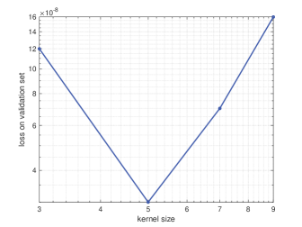
Figure 5: Left: loss on validation set versus $n$. Right: loss on validation set versus kernel size.

In order to assess the performance of CAE-CSI model, the reduced-order solutions are compared with the corresponding DGTD high-fidelity solutions on the test parameter set $\mathcal{P}_{h}^{te}=\{\boldsymbol{\mu}_{1},\boldsymbol{\mu}_{2},\boldsymbol{\mu}_{3},\boldsymbol{\mu}_{4}\}$ where $\boldsymbol{\mu}_{1}=\varepsilon_{1}=1.215,\boldsymbol{\mu}_{2}=\varepsilon_{2}=2.215,\boldsymbol{\mu}_{3}=\varepsilon_{3}=3.215$ and $\boldsymbol{\mu}_{4}=\varepsilon_{4}=4.215$. Firstly, Fig. 6 shows the exact reduced-order matrices and approximate reduced-order matrices based on CSI. Over the Fourier domain during the last oscillation period of the incident wave, we display in Fig. 7 the 1-D $x$-wise evolution along $y=0$ of the real part of $H_{y}$ and $E_{z}$, as well as their 2-D distribution in Fig. 8 and Fig. 9. The time evolution of the relative projection error $e_{\mathbf{u},\rm{Pro}}$ and CAE-CSI error $e_{\mathbf{u},\rm{CAE-CSI}}(\mathbf{u}\in\{\mathbf{E},\mathbf{H}\})$ for the test parameter instances $\boldsymbol{\mu}_{1},\boldsymbol{\mu}_{2},\boldsymbol{\mu}_{3}$ and $\boldsymbol{\mu}_{4}$ are shown in Fig. 10. The average relative error $\bar{e}_{\mathbf{u},\rm{Pro}}$ and $\bar{e}_{\mathbf{u},\rm{CAE-CSI}}(\mathbf{u}\in\{\mathbf{E},\mathbf{H}\})$ for the four test parameters are shown in Tab. 3. It can be seen that the reduced-order solutions and the DGTD solutions match each other very well. Secondly, Tab. 4 presents the time performance comparison of DGTD and CAE-CSI, where we record the average online test time of DGTD solver and ROM for the above four test cases, as well as the training time of the CAE-CSI model. It is worthwhile to take a long time to build a surrogate model, since the online test time of the ROM is greatly shorten compared to the DGTD solver, achieving a speed-up of 3387. Note that the online test time of CAE-CSI is shortened compared to previous work (POD-CSI) [30].

Table 3: Scattering of a plane wave by a dielectric disk. Average relative error on the test set.

$\bar{e}_{\mathbf{H},\rm{Pro}}$	$\bar{e}_{\mathbf{H},\rm{CAE-CSI}}$	$\bar{e}_{\mathbf{E},\rm{Pro}}$	$\bar{e}_{\mathbf{E},\rm{CAE-CSI}}$
1.15%	1.37%	1.56%	1.69%

Table 4: Scattering of a plane wave by a dielectric disk. Comparison between the CAE-CSI (offline and online) and DGTD methods in terms of CPU time. The unit of time is second.

	Offline		Online
Snapshots	Two-step POD	CAE-CSI	CAE-CSI	POD-CSI	DGTD
$2.088\times 10^{4}$	$6.0530$	$1.9042\times 10^{3}$	$0.0761$	$0.2561$	$2.5778\times 10^{2}$

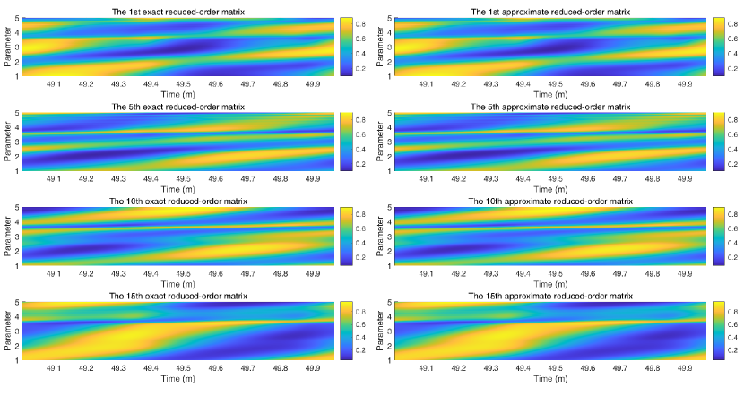
Figure 6: Scattering of a plane wave by a dielectric disk. The 1-st, 5-th, 10-th, and 15-th exact and approximate reduced-order matrices based on CSI.

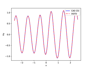
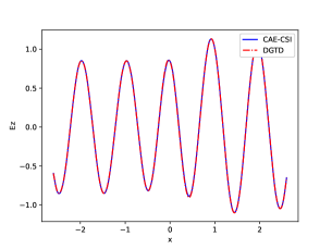
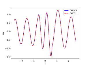
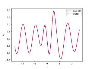
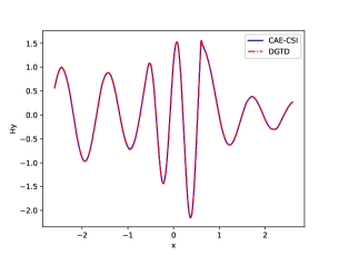
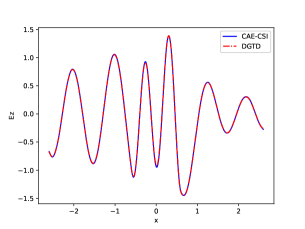
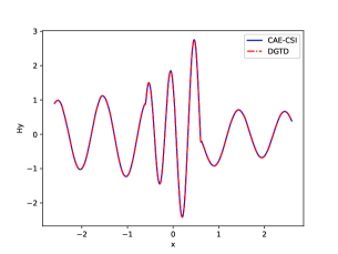
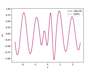
Figure 7: Scattering of a plane wave by a dielectric disk. Comparison of the 1-D $x$-wise distribution along $y=0$ of the real part of $H_{y}$ (left) and $E_{z}$ (right) for the testing parameter instances: $\varepsilon_{1}=1.215$ (1st row), $\varepsilon_{2}=2.215$ (2th row), $\varepsilon_{3}=3.215$ (3th row), $\varepsilon_{4}=4.215$ (4th row).

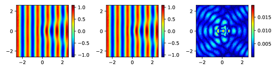
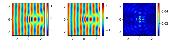
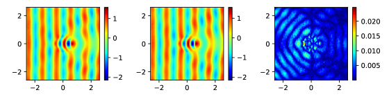
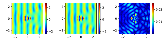
Figure 8: Scattering of a plane wave by a dielectric disk. Comparison of the 2-D distribution of the real part of $H_{y}$ between DGTD (left), CAE-CSI (middle) and relative error (right) for the testing parameter instances: $\varepsilon_{1}=1.215$ (1st row), $\varepsilon_{2}=2.215$ (2th row), $\varepsilon_{3}=3.215$ (3th row), $\varepsilon_{4}=4.215$ (4th row).

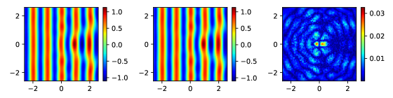
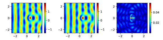
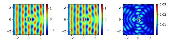
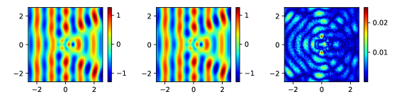
Figure 9: Scattering of a plane wave by a dielectric disk. Comparison of the 2-D distribution of the real part of $E_{z}$ between DGTD (left), CAE-CSI (middle) and relative error (right) for the testing parameter instances: $\varepsilon_{1}=1.215$ (1st row), $\varepsilon_{2}=2.215$ (2th row), $\varepsilon_{3}=3.215$ (3th row), $\varepsilon_{4}=4.215$ (4th row).

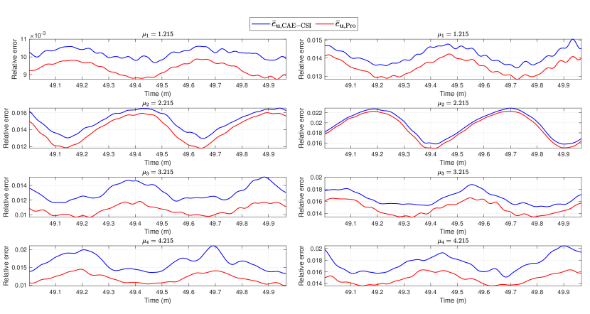
Figure 10: Scattering of a plane wave by a dielectric disk. Comparison of the relative error between DGTD and CAE-CSI for the field $\mathbf{H}$ (left) and $\mathbf{E}$ (right) with the testing parameter instances $\varepsilon_{1}=1.215$ (1st row), $\varepsilon_{2}=2.215$ (2th row), $\varepsilon_{3}=3.215$ (3th row), $\varepsilon_{4}=4.215$ (4th row).

6.2 Scattering of a plane wave by a multi-layer heterogeneous medium

In this subsection, we consider a multi-layer heterogeneous medium which is illuminated by an incident plane wave as shown in Fig. 11. The computational domain is artificially bounded by a square $\Omega=[-3.2\mathrm{~{}m},3.2\mathrm{~{}m}]\times[-3.2\mathrm{~{}m},3.2\mathrm{~{}m}]$ where we impose the Silver-Müller ABC boundary condition. Tab. 5 summarizes the distribution and range of material parameters considered in this study.The mesh consists of 3256 nodes and 6206 elements, resulting in $\mathcal{N}_{h}=37236$ DOFs of the FOM.

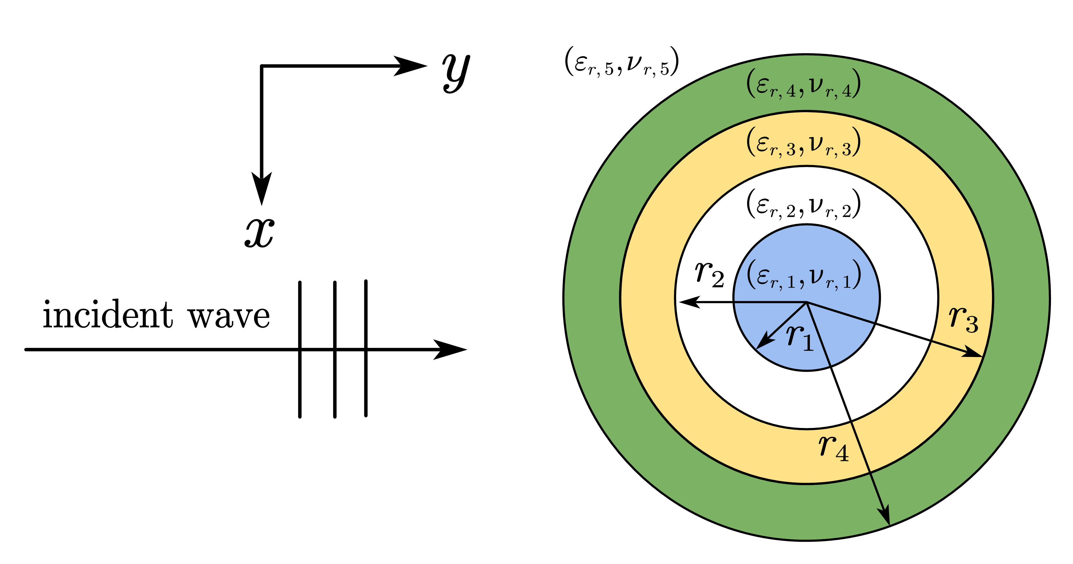
Figure 11: Scattering of plane wave by a multi-layer heterogeneous medium. Geometry of the multi-layer heterogeneous medium.

Table 5: Scattering of plane wave by a multi-layer heterogeneous medium. Distribution and range of material parameters.

Layer $i$	$\mathcal{P}^{i}$	$\nu_{r,i}$	$r_{i}$
1	$\varepsilon_{r,1}\in[5.0,5.6]$	1.0	0.15
2	$\varepsilon_{r,2}\in[3.25,3.75]$	1.0	0.3
3	$\varepsilon_{r,3}\in[2.0,2.5]$	1.0	0.45
4	$\varepsilon_{r,4}\in[1.25,1.75]$	1.0	0.6

The DGTD solver is used to generate the snapshots, and the numerical simulation time is set to 50 periods of the incident wave oscillation with time step $\Delta t=0.0038$ s for each 4-dimensional parameter $\boldsymbol{\mu}\in\mathcal{P}$, where $\mathcal{P}=\mathcal{P}^{1}\times\mathcal{P}^{2}\times\mathcal{P}^{3}\times\mathcal{P}^{4}\subset\mathbb{R}^{4}$ with $\varepsilon_{r,i}\in\mathcal{P}^{i}$ $(i=1,2,3,4)$. We adopt a grid sampling of tensor product with $\mathcal{N}_{\Delta p}=3$ uniform points for each parameter to form a training parameter samples $\mathcal{P}_{h}^{tr}$, resulting in $\mathcal{N}_{p}=81$ points. Each choice of the parameter is sampled for $\mathcal{N}_{t}=253$ snapshots in time at the last period, i.e., $\mathcal{T}_{h}^{tr}=\{49.0002,49.0041,\cdots,49.9630,49.9669\}$. Fig. 12 shows the convergence histories of $\bar{e}_{\mathbf{H},\rm{POD}}$ and $\bar{e}_{\mathbf{E},\rm{POD}}$ with different truncation parameter $k$ and size parameter $\mathcal{N}$ in the two-step POD method. The POD basis matrices $\mathbf{V}_{\mathbf{u}}\ (\mathbf{u}\in\{\mathbf{E},\mathbf{H}\})$ are generated by the two-step POD method with $k=4$ and $\mathcal{N}=196$. The architecture of the CAE network is the same as the one used in the first experiment. After performing a SVD to all reduced-order matrices with a truncation tolerance $\delta=1\times 10^{-4}$, the CSI models are built as the combination of time- and parameter-modes. To evaluate the CAE-CSI method, we compare the reduced-order solution with the high-fidelity solution generated by the DGTD method on a test parameter set $\mathcal{P}_{h}^{te}=\{\boldsymbol{\mu}_{1},\boldsymbol{\mu}_{2},\boldsymbol{\mu}_{3}\}$ with $\boldsymbol{\mu}_{1}=\{(5.1,3.4,2.1,1.4)\}$, $\boldsymbol{\mu}_{2}=\{(5.4,3.4,2.3,1.3)\}$ and $\boldsymbol{\mu}_{3}=\{(5.5,3.7,2.4,1.7)\}$. Fig. 13 shows the 1-D $x$-wise distribution along $y=0$ of the real part of $H_{y}$ and $E_{z}$ in the Fourier domain on the last period of simulation. Fig. 14 and Fig. 15 display the 2-D distribution of the real part of $H_{y}$ and $E_{z}$. The time evolution of the relative projection error $e_{\mathbf{u},\rm{Pro}}$ and CAE-CSI error $e_{\mathbf{u},\rm{CAE-CSI}}(\mathbf{u}\in\{\mathbf{E},\mathbf{H}\})$ for 3 test parameters $\boldsymbol{\mu}_{1},\boldsymbol{\mu}_{2}$ and $\boldsymbol{\mu}_{3}$ are displayed in Fig. 16. The average projection error $\bar{e}_{\mathbf{u},\rm{Pro}}$ and the average CAE-CSI error $\bar{e}_{\mathbf{u},\rm{CAE-CSI}}(\mathbf{u}\in\{\mathbf{E},\mathbf{H}\})$ for the 3 test parameters are listed in Tab. 6.

Table 6: Scattering of plane wave by a multi-layer heterogeneous medium. Average relative error on the test set.

$\bar{e}_{\mathbf{H},\rm{Pro}}$	$\bar{e}_{\mathbf{H},\rm{CAE-CSI}}$	$\bar{e}_{\mathbf{E},\rm{Pro}}$	$\bar{e}_{\mathbf{E},\rm{CAE-CSI}}$
0.60%	0.89%	0.69%	1.03%

Performance results of the CAE-CSI and DGTD methods with $\mathbb{P}_{2}$ approximation are summarized in Tab. 7. The CPU time of the DGTD method is $3.0477\times 10^{2}$ s and the online cost of the CAE-CSI is 0.2923 s, corresponding to a speed-up of 1042. Note that the online test time of CAE-CSI is again shortened compared to previous work (POD-CSI) [30], which again demonstrates the significantly enhanced efficiency of the CAE-CSI method.

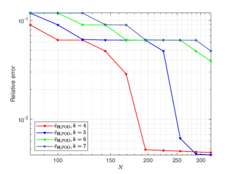
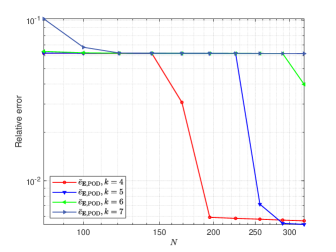
Figure 12: Scattering of plane wave by a multi-layer heterogeneous medium. Convergence histories of $\bar{e}_{\mathbf{H},\rm{POD}}$ (left) and $\bar{e}_{\mathbf{E},\rm{POD}}$ (right) with the choice of $k$ and $\mathcal{N}$.

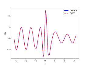
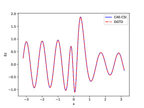
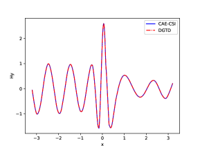
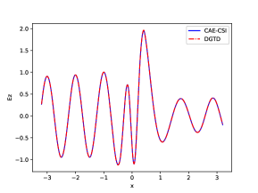
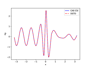
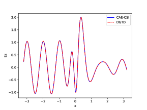
Figure 13: Scattering of plane wave by a multi-layer heterogeneous medium. Comparison of the 1-D $x$-wise distribution along $y=0$ of the real part of $H_{y}$ (left) and $E_{z}$ (right) for the testing parameter instances: $\boldsymbol{\mu}_{1}=\{(5.1,3.4,2.1,1.4)\}$ (1st row), $\boldsymbol{\mu}_{2}=\{(5.4,3.4,2.3,1.3)\}$ (2th row) and $\boldsymbol{\mu}_{3}=\{(5.5,3.7,2.4,1.7)\}$ (3th row).

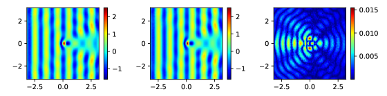
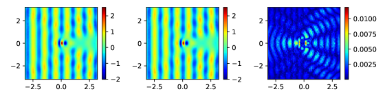
Figure 14: Scattering of plane wave by a multi-layer heterogeneous medium. Comparison of the 2-D distribution of the real part of $H_{y}$ between DGTD (left), CAE-CSI (middle) and relative error (right) for the testing parameter instances: $\boldsymbol{\mu}_{1}=\{(5.1,3.4,2.1,1.4)\}$ (1st row), $\boldsymbol{\mu}_{2}=\{(5.4,3.4,2.3,1.3)\}$ (2th row) and $\boldsymbol{\mu}_{3}=\{(5.5,3.7,2.4,1.7)\}$ (3th row).

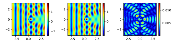
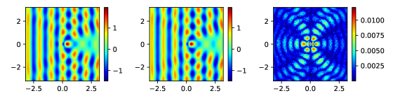
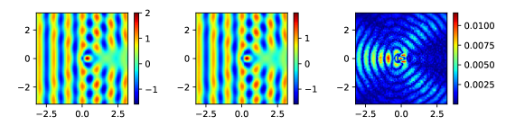
Figure 15: Scattering of plane wave by a multi-layer heterogeneous medium: comparison of the 2-D distribution of the real part of $E_{z}$ between DGTD (left), CAE-CSI (middle) and relative error (right) for the testing parameter instances: $\boldsymbol{\mu}_{1}=\{(5.1,3.4,2.1,1.4)\}$ (1st row), $\boldsymbol{\mu}_{2}=\{(5.4,3.4,2.3,1.3)\}$ (2th row) and $\boldsymbol{\mu}_{3}=\{(5.5,3.7,2.4,1.7)\}$ (3th row).

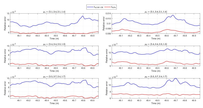
Figure 16: Scattering of plane wave by a multi-layer heterogeneous medium. Comparison of the relative projection error $e_{\mathbf{u},\rm{Pro}}$, the CAE-CSI error $e_{\mathbf{u},\rm{CAE-CSI}}$ for $\mathbf{H}$ (left) and $\mathbf{E}$ (right) for the testing parameter instances: $\boldsymbol{\mu}_{1}=\{(5.1,3.4,2.1,1.4)\}$ (1st row), $\boldsymbol{\mu}_{2}=\{(5.4,3.4,2.3,1.3)\}$ (2th row) and $\boldsymbol{\mu}_{3}=\{(5.5,3.7,2.4,1.7)\}$ (3th row).

Table 7: Scattering of plane wave by a multi-layer heterogeneous medium. Comparison between the CAE-CSI (offline and online) and DGTD methods in terms of CPU time. The unit of time is second.

	Offline		Online
Snapshots	Two-step POD	CAE-CSI	CAE-CSI	POD-CSI	DGTD
$2.4686\times 10^{4}$	6.5544	$2.0432\times 10^{3}$	$0.2923$	$1.4856$	$3.0477\times 10^{2}$

7 Conclusion

A data-driven RB method based on POD, CAE and CSI is proposed to accelerate the solution of parameterized time-domain Maxwell equations. The two-step POD method performs a prior dimensionality reduction of the snapshots, then the CAE network provides a low dimensional representation of the projection coefficients through its encoder, as well as the inverse map through its decoder. CSI-based models are trained to approximate a mapping from the time/parameters to the low dimensional representations and the decoder is used to reconstruct the system solutions to their original dimension. By combining CSI with a decoder, a ‘simulation-free’ approach is established to obtain a RB solution at a very low cost. The results of the numerical experiments demonstrate the powerful dimensionality reduction and reconstruction capabilities of the CAE-CSI method, and a highly accurate and cheap surrogate model for systems described by PDEs is developed. Future research directions include more realistic 3-D simulations and the reduction of parameterized geometry.

References

- [1] G Hossein Behforooz. A comparison of theE (3) and not-a-knot cubic splines. Appl. Math. Comput., 72(2-3):219–223, 1995.
- [2] Yoshua Bengio, Aaron Courville, and Pascal Vincent. Representation learning: A review and new perspectives. IEEE Trans. Pattern Anal. Mach. Intell., 35(8):1798–1828, 2013.
- [3] Peter Benner, Mario Ohlberger, Anthony Patera, Gianluigi Rozza, and Karsten Urban. Model reduction of parametrized systems. Springer, 2017.
- [4] T Bui-Thanh, Murali Damodaran, and Karen Willcox. Proper orthogonal decomposition extensions for parametric applications in compressible aerodynamics. In Proceedings of the 21st AIAA Applied Aerodynamics Conference, page 4213, 2003.
- [5] Wenqian Chen, Qian Wang, Jan S Hesthaven, and Chuhua Zhang. Physics-informed machine learning for reduced-order modeling of nonlinear problems. J. Comput. Phys., 446:110666, 2021.
- [6] Vincent Dumoulin and Francesco Visin. A guide to convolution arithmetic for deep learning. arXiv preprint arXiv:1603.07285, 2016.
- [7] Carl Eckart and Gale Young. The approximation of one matrix by another of lower rank. Psychometrika, 1(3):211–218, 1936.
- [8] Loula Fezoui, Stéphane Lanteri, Stéphanie Lohrengel, and Serge Piperno. Convergence and stability of a discontinuous Galerkin time-domain method for the 3D heterogeneous Maxwell equations on unstructured meshes. ESAIM: Math. Model. Numer. Anal., 39(6):1149–1176, 2005.
- [9] Stefania Fresca and Andrea Manzoni. POD-DL-ROM: enhancing deep learning-based reduced order models for nonlinear parametrized PDEs by proper orthogonal decomposition. Comput. Methods Appl. Mech. Eng., 388:114181, 2022.
- [10] Stephen D Gedney. Introduction to the finite-difference time-domain (FDTD) method for electromagnetics. Synthesis Lectures on Computational Electromagnetics, 6(1):1–250, 2011.
- [11] Xavier Glorot and Yoshua Bengio. Understanding the difficulty of training deep feedforward neural networks. In Proceedings of the 13th International Conference on Artificial Intelligence and Statistics, pages 249–256. JMLR Workshop and Conference Proceedings, 2010.
- [12] Francisco J Gonzalez and Maciej Balajewicz. Deep convolutional recurrent autoencoders for learning low-dimensional feature dynamics of fluid systems. arXiv preprint arXiv:1808.01346, 2018.
- [13] Mengwu Guo and Jan S Hesthaven. Reduced order modeling for nonlinear structural analysis using Gaussian process regression. Comput. Methods Appl. Mech. Eng., 341:807–826, 2018.
- [14] Mengwu Guo and Jan S Hesthaven. Data-driven reduced order modeling for time-dependent problems. Comput. Methods Appl. Mech. Eng., 345:75–99, 2019.
- [15] Xiaoxiao Guo, Wei Li, and Francesco Iorio. Convolutional neural networks for steady flow approximation. In Proceedings of the 22nd ACM SIGKDD International Conference on Knowledge Discovery and Data Mining, pages 481–490, 2016.
- [16] Md Sakib Hasan, Sherif Amer, Syed K Islam, and Garrett S Rose. Multivariate cubic spline: a versatile DC modeling technique suitable for different deep submicron transistors. In Proceedings of the 2019 IEEE SoutheastCon Conference, pages 1–8. IEEE, 2019.
- [17] Md Sakib Hasan, Syed K Islam, and Benjamin J Blalock. Modeling of SOI four-gate transistor (G4FET) using multidimensional spline interpolation method. Microelectronics J., 76:33–42, 2018.
- [18] Jan S Hesthaven, Gianluigi Rozza, Benjamin Stamm, et al. Certified reduced basis methods for parametrized partial differential equations, volume 590. Springer, 2016.
- [19] Jan S Hesthaven and Stefano Ubbiali. Non-intrusive reduced order modeling of nonlinear problems using neural networks. J. Comput. Phys., 363:55–78, 2018.
- [20] Jan S Hesthaven and Tim Warburton. Nodal discontinuous Galerkin methods: algorithms, analysis, and applications. Springer Science & Business Media, 2007.
- [21] Sergey Ioffe and Christian Szegedy. Batch normalization: Accelerating deep network training by reducing internal covariate shift. In Proceedings of the 32nd International Conference on Machine Learning, pages 448–456. PMLR, 2015.
- [22] Jian-Ming Jin. Theory and computation of electromagnetic fields. John Wiley & Sons, 2011.
- [23] Mariella Kast, Mengwu Guo, and Jan S Hesthaven. A non-intrusive multifidelity method for the reduced order modeling of nonlinear problems. Comput. Methods Appl. Mech. Eng., 364:112947, 2020.
- [24] Diederik P Kingma and Jimmy Ba. Adam: A method for stochastic optimization. arXiv preprint arXiv:1412.6980, 2014.
- [25] Yann LeCun, Léon Bottou, Yoshua Bengio, and Patrick Haffner. Gradient-based learning applied to document recognition. Proc. IEEEE, 86(11):2278–2324, 1998.
- [26] Kookjin Lee and Kevin T Carlberg. Model reduction of dynamical systems on nonlinear manifolds using deep convolutional autoencoders. J. Comput. Phys., 404:108973, 2020.
- [27] Jichun Li and Bing Nan. Simulating backward wave propagation in metamaterial with radial basis functions. Results Appl. Math., 2:100009, 2019.
- [28] Kun Li, Ting-Zhu Huang, Liang Li, and Stéphane Lanteri. A reduced-order DG formulation based on POD method for the time-domain Maxwell’s equations in dispersive media. J. Comput. Appl. Math., 336:249–266, 2018.
- [29] Kun Li, Ting-Zhu Huang, Liang Li, and Stéphane Lanteri. Pod-based model order reduction with an adaptive snapshot selection for a discontinuous galerkin approximation of the time-domain maxwell’s equations. J. Comput. Phys., 396:106–128, 2019.
- [30] Kun Li, Ting-Zhu Huang, Liang Li, and Stéphane Lanteri. Non-intrusive reduced-order modeling of parameterized electromagnetic scattering problems using cubic spline interpolation. J. Sci. Comput., 87(2):1–29, 2021.
- [31] Lu Lu, Xuhui Meng, Zhiping Mao, and George Em Karniadakis. DeepXDE: A deep learning library for solving differential equations. SIAM Review, 63(1):208–228, 2021.
- [32] Luke Melas-Kyriazi. The mathematical foundations of manifold learning. arXiv preprint arXiv:2011.01307, 2020.
- [33] Peter Monk et al. Finite element methods for Maxwell’s equations. Oxford University Press, 2003.
- [34] Stefanos Nikolopoulos, Ioannis Kalogeris, and Vissarion Papadopoulos. Non-intrusive surrogate modeling for parametrized time-dependent partial differential equations using convolutional autoencoders. Eng. Appl. Artif. Intell., 109:104652, 2022.
- [35] M Oulghelou and C Allery. Non intrusive method for parametric model order reduction using a bi-calibrated interpolation on the grassmann manifold. J. Comput. Phys., 426:109924, 2021.
- [36] Adam Paszke, Sam Gross, Francisco Massa, Adam Lerer, James Bradbury, Gregory Chanan, Trevor Killeen, Zeming Lin, Natalia Gimelshein, Luca Antiga, et al. Pytorch: An imperative style, high-performance deep learning library. Adv. Neural Inf. Process Syst., 32, 2019.
- [37] Maziar Raissi, Paris Perdikaris, and George E Karniadakis. Physics-informed neural networks: A deep learning framework for solving forward and inverse problems involving nonlinear partial differential equations. J. Comput. Phys., 378:686–707, 2019.
- [38] E Schmidt. On the theory of linear and nonlinear integral equations. i. development of arbitrary function according to systems prescribed. Math. Ann., 63:433–476, 1907.
- [39] Allen Taflove and Susan Hagness. Computational electrodynamics: the finite-difference time-domain method - 3rd ed. Artech House Publishers, 2005.
- [40] Jonathan Viquerat. Simulation of electromagnetic waves propagation in nano-optics with a high-order discontinuous Galerkin time-domain method. PhD thesis, Université Nice Sophia Antipolis, 2015.
- [41] Qian Wang, Jan S Hesthaven, and Deep Ray. Non-intrusive reduced order modeling of unsteady flows using artificial neural networks with application to a combustion problem. J. Comput. Phys., 384:289–307, 2019.
- [42] Ren-Hong Wang. Multivariate spline functions and their applications, volume 529. Springer Science & Business Media, 2013.
- [43] D Xiao, F Fang, CC Pain, and IM Navon. A parameterized non-intrusive reduced order model and error analysis for general time-dependent nonlinear partial differential equations and its applications. Comput. Methods Appl. Mech. Eng., 317:868–889, 2017.
- [44] Dunhui Xiao, Fangxin Fang, Andrew G Buchan, Christopher C Pain, Ionel M Navon, and Ann Muggeridge. Non-intrusive reduced order modelling of the Navier–Stokes equations. Comput. Methods Appl. Mech. Eng., 293:522–541, 2015.
- [45] Qiang Ye and Weifeng Zhi. Discrete Hessian eigenmaps method for dimensionality reduction. J. Comput. Appl. Math., 278:197–212, 2015.
- [46] Kane Yee. Numerical solution of initial boundary value problems involving Maxwell’s equations in isotropic media. IEEE Trans. Antennas Propag., 14(3):302–307, 1966.
- [47] Aston Zhang, Zachary C Lipton, Mu Li, and Alexander J Smola. Dive into deep learning. arXiv preprint arXiv:2106.11342, 2021.
- [48] Ying Zhao, Liang Li, and Kun Li. Non-intrusive reduced order modeling of parametric electromagnetic scattering problems through Gaussian process regression. arXiv preprint arXiv:2103.12472, 2021.
- [49] Tong Zhou and Yongbo Peng. Kernel principal component analysis-based Gaussian process regression modelling for high-dimensional reliability analysis. Comput. Struct., 241:106358, 2020.