Curve Simplification and Clustering
under Fréchet Distance

We present new approximation results on curve simplification and clustering under Fréchet distance. Let $T=\{\tau_{i}:i\in[n]\}$ be polygonal curves in $\mathbb{R}^{d}$ of $m$ vertices each. Let $\ell$ be any integer from $[m]$. We study a generalized curve simplification problem: given error bounds $\delta_{i}>0$ for $i\in[n]$, find a curve $\sigma$ of at most $\ell$ vertices such that $d_{F}(\sigma,\tau_{i})\leq\delta_{i}$ for $i\in[n]$. We present an algorithm that returns a null output or a curve $\sigma$ of at most $\ell$ vertices such that $d_{F}(\sigma,\tau_{i})\leq\delta_{i}+\varepsilon\delta_{\max}$ for $i\in[n]$, where $\delta_{\max}=\max_{i\in[n]}\delta_{i}$. If the output is null, there is no curve of at most $\ell$ vertices within a Fréchet distance of $\delta_{i}$ from $\tau_{i}$ for $i\in[n]$. The running time is $\tilde{O}\bigl{(}n^{O(\ell)}\cdot m^{O(\ell^{2})}\cdot(d\ell/\varepsilon)^{O(d\ell)}\bigr{)}$. This algorithm yields the first polynomial-time bicriteria approximation scheme to simplify a curve $\tau$ to another curve $\sigma$, where the vertices of $\sigma$ can be anywhere in $\mathbb{R}^{d}$, so that $d_{F}(\sigma,\tau)\leq(1+\varepsilon)\delta$ and $|\sigma|\leq(1+\alpha)\cdot\min\{|c|:d_{F}(c,\tau)\leq\delta\}$ for any given $\delta>0$ and any fixed $\alpha,\varepsilon\in(0,1)$. The running time is $\tilde{O}\bigl{(}m^{O(1/\alpha)}\cdot(d/(\alpha\varepsilon))^{O(d/\alpha)}\bigr{)}$. By combining our technique with some previous results in the literature, we obtain an approximation algorithm for $(k,\ell)$-median clustering. Given $T$, it computes a set $\Sigma$ of $k$ curves, each of $\ell$ vertices, such that $\sum_{i\in[n]}\min_{\sigma\in\Sigma}d_{F}(\sigma,\tau_{i})$ is within a factor $1+\varepsilon$ of the optimum with probability at least $1-\mu$ for any given $\mu,\varepsilon\in(0,1)$. The running time is $\tilde{O}\bigl{(}n\cdot m^{O(k\ell^{2})}\cdot\mu^{-O(k\ell)}\cdot(dk\ell/\varepsilon)^{O((dk\ell/\varepsilon)\log(1/\mu))}\bigr{)}$.

1 Introduction

The popularity of trajectory data analysis in applications such as wildlife monitoring, delivery tracking, and transportation analysis has generated a lot of interest in curve simplification and clustering under the Fréchet distance $d_{F}$. Given a polygonal curve $\tau$ of $m$ vertices in $\mathbb{R}^{d}$ and a value $\delta>0$, curve simplification calls for computing a polygonal curve $\sigma$ of fewer vertices such that $d_{F}(\sigma,\tau)\leq\delta$. Given a set of polygonal curves $T$ and two positive integers $k$ and $\ell$, the $(k,\ell)$-clustering problem is to find a set $\Sigma$ of $k$ curves, each of $\ell$ vertices, that minimizes some distance measure between $\Sigma$ and $T$. We present new approximation results for both problems.

Previous works. Alt and Godau [2] developed the first algorithm for computing $d_{F}(\sigma,\tau)$; it runs in $O\bigl{(}|\sigma||\tau|\log(|\sigma||\tau|)\bigr{)}$ time, where $|\sigma|$ and $|\tau|$ denote their numbers of vertices. Let $\kappa(\tau,\delta)=\min\{|c|:d_{F}(c,\tau)\leq\delta\}$. Let $m$ be $|\tau|$. Agarwal et al. [1] named this problem as weak Fréchet $\delta$-simplification and proposed an $O(m\log m)$-time algorithm in $\mathbb{R}^{2}$ that returns a curve $\sigma$ such that $d_{F}(\sigma,\tau)\leq\delta$ and $|\sigma|\leq\kappa(\tau,\delta/4)$ for a given $\delta>0$. Guibas et al. [9] presented an $O(m^{2}\log^{2}m)$-time algorithm that minimizes $|\sigma|$ such that $d_{F}(\sigma,\tau)\leq\delta$ in $\mathbb{R}^{2}$. But in $\mathbb{R}^{d}$ with $d\geq 3$, no algorithm is known yet. Van Kreveld et al. [12] can minimize $|\sigma|$ in $O(|\sigma|m^{5})$ time under the constraints of $d_{F}(\sigma,\tau)\leq\delta$ for a given $\delta>0$ and the vertices of $\sigma$ being a subset of the vertices of $\tau$. Van de Kerkhof et al. [11] improved the running time to $O(m^{3})$—a result also obtained by Bringmann and Chaudhury [3]—and that the problem is NP-hard for $d\geq 2$ if the vertices of $\sigma$ can be anywhere on $\tau$. Van de Kerkhof et al. proposed another algorithm that returns a curve $\sigma$ in $O(\mathrm{poly}(1/\varepsilon)\cdot m^{2}\log m\log\log m)$ time such that $d_{F}(\sigma,\tau)\leq(1+\varepsilon)\delta$ and $|\sigma|\leq 2\kappa(\tau,\delta)-2$, if the vertices of $\sigma$ can be anywhere in $\mathbb{R}^{d}$.

Let $T$ be a set of $n$ polygonal curves in $\mathbb{R}^{d}$, each of $m$ vertices. The $(k,\ell)$-center clustering problem is to find a set $\Sigma$ of $k$ curves, each of $\ell$ vertices, such that $\max_{\tau\in T}\min_{\sigma\in\Sigma}d_{F}(\sigma,\tau)$ is minimized. The $(k,\ell)$-median clustering problem is to minimize $\sum_{\tau\in T}\min_{\sigma\in\Sigma}d_{F}(\sigma,\tau)$. Driemel et al. [8] initiated the study of $(k,\ell)$-center clustering; they obtained approximation ratios of $1+\varepsilon$ in one dimension and 8 in higher dimensions. Buchin et al. [4] proved that if $\ell$ is part of the input, there is no polynomial-time approximation scheme for $d\geq 2$ unless P = NP; if both $k$ and $\ell$ are constants, a lower bound of $2.25-\epsilon$ on the approximation ratio is shown. Buchin et al. also obtained smaller constant factor approximations for $d\geq 2$. It is worth noting that the hardness results [4] of the $(1,\ell)$-center problem imply that the generalized curve simplification problem is also NP-hard and hard to approximate with a small constant factor. For $(k,\ell)$-median clustering, Buchin et al. [5] proved that the problem is NP-hard even if $k=1$. Subsequently, Buchin et al. [6] designed a randomized bicriteria approximation algorithm; it computes a set $\Sigma$ of $k$ curves that has a cost at most $1+\varepsilon$ times the optimum with probability at least $1-\mu$. Each curve in $\Sigma$ may have up to $2\ell-2$ vertices. The running time is $\tilde{O}\bigl{(}n\cdot m^{O(k\ell)}\cdot 2^{O((k^{3}/\varepsilon^{2})\log^{2}(1/\mu))}\cdot(k/(\mu\varepsilon))^{O(dk\ell)}\bigr{)}$. There are some results on coresets for $(k,\ell)$-median clustering under Fréchet distance [7].

Our results. Let $T=\{\tau_{i}:i\in[n]\}$ be polygonal curves in $\mathbb{R}^{d}$ of $m$ vertices each. Let $\ell$ be any integer from $[m]$. We study a generalized curve simplification problem: given error bounds $\delta_{i}>0$ for $i\in[n]$, find a curve $\sigma$ of at most $\ell$ vertices such that $d_{F}(\sigma,\tau_{i})\leq\delta_{i}$ for $i\in[n]$. We present an algorithm that returns a null output or a curve $\sigma$ of at most $\ell$ vertices such that $d_{F}(\sigma,\tau_{i})\leq\delta_{i}+\varepsilon\delta_{\max}$ for $i\in[n]$, where $\delta_{\max}=\max_{i\in[n]}\delta_{i}$. If the output is null, there is no curve of at most $\ell$ vertices within a Fréchet distance of $\delta_{i}$ from $\tau_{i}$ for $i\in[n]$. The running time is $\tilde{O}\bigl{(}n^{O(\ell)}\cdot m^{O(\ell^{2})}\cdot(d\ell/\varepsilon)^{O(d\ell)}\bigr{)}$.

This algorithm also yields a polynomial-time bicriteria approximation scheme to simplify a curve $\tau$ to another curve $\sigma$, where the vertices of $\sigma$ can be anywhere in $\mathbb{R}^{d}$, so that $d_{F}(\sigma,\tau)\leq(1+\varepsilon)\delta$ and $|\sigma|\leq(1+\alpha)\kappa(\tau,\delta)$ given any $\delta>0$ and any $\alpha,\varepsilon\in(0,1)$. The running time is $\tilde{O}\bigl{(}m^{O(1/\alpha)}\cdot(d/(\alpha\varepsilon))^{O(d/\alpha)}\bigr{)}$. This is the first polynomial-time bicriteria approximation scheme for simplifying a curve in $\mathbb{R}^{d}$ with $d\geq 3$.

By combining our technique with the framework in [6], we obtain an approximation algorithm for $(k,\ell)$-median clustering. Given $T$, it computes a set $\Sigma$ of $k$ curves, each of $\ell$ vertices, such that $\sum_{i\in[n]}\min_{\sigma\in\Sigma}d_{F}(\sigma,\tau_{i})$ is within a factor $1+\varepsilon$ of the optimum with probability at least $1-\mu$ for any given $\mu,\varepsilon\in(0,1)$. The running time is $\tilde{O}\bigl{(}n\cdot m^{O(k\ell^{2})}\cdot\mu^{-O(k\ell)}\cdot(dk\ell/\varepsilon)^{O((dk\ell/\varepsilon)\log(1/\mu))}\bigr{)}$. This result answers affirmatively the question raised in the previous work [6], which guarantees a bound of $2\ell-2$ on the output curve sizes, of whether the bound $\ell$ can be achieved with similar efficiency.

There are two main ingredients of our results. The first one is a space of configurations. We use the grids introduced by Buchin et al. [6] as a part of our discretization scheme; however, instead of enumerating all possible curves through the discretization vertices, we define configurations with some novel structural constraints in order to satisfy the bound $\ell$ on the size of the output curves. Second, we design a two-phase method to construct approximate curves from the configurations.

Notations. We often denote a curve $\sigma$ as a sequence $(u_{1},u_{2},\ldots,u_{l})$ of its vertices. Given two points $x,y$ on $\sigma$, we say that $x\leq_{\sigma}y$ if $y$ is not encountered before $x$ as we walk along $\sigma$ from $u_{1}$. Given two subsets $X$ and $Y$ of points on $\sigma$, we say that $X\leq_{\sigma}Y$ if $x\leq_{\sigma}y$ for all $x\in X$ and $y\in Y$.

A parameterization of $\sigma$ is a continuous function $\rho:[0,1]\rightarrow\sigma$ such that $\rho(0)=u_{1}$, $\rho(1)=u_{l}$, and for all $t,t^{\prime}\in[0,1]$, $t\leq t^{\prime}\iff\rho(t)\leq_{\sigma}\rho(t^{\prime})$. A matching $g$ from a curve $\sigma$ to another curve $\tau$ is a pair of parameterizations $(\rho,\rho^{\prime})$ for $\sigma$ and $\tau$, respectively, and $d_{g}(\sigma,\tau)=\max_{t\in[0,1]}d(\rho(t),\rho^{\prime}(t))$. For any point $x\in\sigma$, we denote the points in $\tau$ matched to $x$ by $g(x)=\bigl{\{}y\in\tau:\exists\,t\in[0,1]\,\,\text{s.t.}\,\,x=\rho(t)\,\wedge\,y=\rho^{\prime}(t)\bigr{\}}$; for a subset $X\subseteq\sigma$, $g(X)=\bigcup_{x\in X}g(x)$. For any point $y\in\tau$, we denote the points in $\sigma$ matched to $y$ by $g^{-1}(y)=\{x\in\sigma:\exists\,t\in[0,1]\,\,\text{s.t.}\,x=\rho(t)\,\wedge\,y=\rho^{\prime}(t)\}$; for a subset $Y\subseteq\tau$, $g^{-1}(Y)=\bigcup_{y\in Y}g^{-1}(y)$. The Fréchet distance of $\sigma$ and $\tau$ is $d_{F}(\sigma,\tau)=\inf_{g}d_{g}(\sigma,\tau)$. A Fréchet matching from $\sigma$ to $\tau$ is a matching that realizes $d_{F}(\sigma,\tau)$. Clearly, $d_{F}(\sigma,\tau)=d_{F}(\tau,\sigma)$.

We will be dealing with a set $T$ of polygonal curves of $m$ vertices each. For each curve $\tau_{i}\in T$, we denote its vertices in order along $\tau_{i}$ by $v_{i,1},\ldots,v_{i,m}$. For all $a\in[m-1]$, $\tau_{i,a}$ denotes the edge $v_{i,a}v_{i,a+1}$. For all $a,b\in[m]$ such that $a\leq b$, $[v_{i,a},v_{i,b}]$ denotes the vertices $\{v_{i,a},v_{i,a+1},\ldots,v_{i,b}\}$. Given two points $x,y$ on a curve $\tau$ such that $x\leq_{\tau}y$, $\tau[x,y]$ denotes the subcurve of $\tau$ from $x$ to $y$.

Given two points $x,y\in\mathbb{R}^{d}$, $xy$ denotes the closed line segment connecting $x$ and $y$. Given any curve $\tau$, $\mathrm{int}(\tau)$ denotes the relative interior of $\tau$. We use $B_{r}$ to denote the ball centered at the origin with radius $r$. Given two subsets $S$ and $S^{\prime}$ of $\mathbb{R}^{d}$, their Minkowski sum is $S\oplus S^{\prime}=\{x+y:x\in S,\,y\in S^{\prime}\}$. Given a point $p$ and $S\subseteq\mathbb{R}^{d}$, $p+S=\{p+x:x\in S\}$. For any point $x$ and any segment $s$, $x\!\downarrow\!s$ denotes the orthogonal projection of $x$ onto the support line of $s$; so $x\!\downarrow\!s$ may not lie on $s$. For a point set $X$, $X\!\downarrow\!s=\{x\!\downarrow\!s:x\in X\}$.

2 Simplified representative of a set of curves

Let $\Delta=\{\delta_{i}:i\in[n]\}$ be a set of error thresholds prescribed for $T$. Define $Q(T,\Delta,\ell)$ to be the problem of finding a curve $\sigma$ of at most $\ell$ vertices such that $d_{F}(\sigma,\tau_{i})\leq\delta_{i}$ for $i\in[n]$.

2.1 Configurations

Imagine an infinite grid of hypercubes of side length $\alpha$. Given a subset $R\subset\mathbb{R}^{d}$, let $G(R,\alpha)$ be the subset of grid cells that intersect $R$.

Let $\min=\mathrm{argmin}_{i\in[n]}\delta_{i}$. We compute $\mathcal{L}=\bigcup_{a\in[m-1]}L_{a}$, where $L_{a}$ is a set of segments that are parallel to $\tau_{\min,a}$. First, compute the convex hull $C_{a}$ of $G(v_{\min,a}+B_{\delta_{\min}},\varepsilon\delta_{\min})\cup G(v_{\min,a+1}+B_{\delta_{\min}},\varepsilon\delta_{\min})$. Second, for every grid vertex $x\in G(v_{\min,a}+B_{\delta_{\min}},\varepsilon\delta_{\min})$, take the line through $x$ that is parallel to $\tau_{\min,a}$, clip this line within $C_{a}$ to a segment, and include this segment in $L_{a}$. The size of $L_{a}$ is $O(\varepsilon^{-d})$; it can be computed in $O(\varepsilon^{-d^{2}/2})$ time. Each point in $C_{a}$ is at distance $\sqrt{d}\varepsilon\delta_{\min}$ or less from a segment in $L_{a}$. The size of $\mathcal{L}$ is $O(m\varepsilon^{-d})$; it can be computed in $O(m\varepsilon^{-d^{2}/2})$ time.

Take any integer $l\in[\ell]$. We construct two sets of grid cells: ${\mathcal{G}}_{1}=\bigcup_{i\in[n]}\bigcup_{a\in[m]}G\bigl{(}v_{i,a}+B_{\delta_{i}+\sqrt{d}\varepsilon\delta_{i}},\varepsilon\delta_{i}/l)$ and ${\mathcal{G}}_{2}=\bigcup_{i\in[n]}\bigcup_{a\in[m]}G\bigl{(}v_{i,a}+B_{9\sqrt{d}\delta_{\max}},\varepsilon\delta_{\max})$, where $\delta_{\max}=\max_{i\in[n]}\delta_{i}$. The size and construction time of ${\mathcal{G}}_{1}$ are $O(mnl^{d}\varepsilon^{-d})$; those of ${\mathcal{G}}_{2}$ are smaller by an $l^{d}$ factor.

Each configuration $\Psi_{l}$ is a 4-tuple $(\mathcal{P},\mathcal{C},\mathcal{S},\mathcal{A})$ designed to capture a candidate curve $\sigma=(w_{1},\ldots,w_{l})$ of $l$ vertices. The component $\mathcal{P}$ is an $n$-tuple $(\pi_{i})_{i\in[n]}$. Each $\pi_{i}$ is a function from $[m]$ to $[0,l-1]$ that partitions the vertices of $\tau_{i}$ into at most $l$ contiguous subsets. If $\pi_{i}(a)=0$, it means that $v_{i,a}$ should be matched to $w_{1}$; if $\pi_{i}(a)=j\in[l-1]$, it means that $v_{i,a}$ should be matched to point(s) in $w_{j}w_{j+1}\setminus\{w_{j}\}$. We require that for all $i\in[n]$, $\pi_{i}(1)=0$ and if $a\leq b$, then $\pi_{i}(a)\leq\pi_{i}(b)$.

The component $\mathcal{C}$ is an $(l-1)$-tuple $((c_{j,1},c_{j,2}))_{j\in[l-1]}$, where $c_{j,1}$ and $c_{j,2}$ are cells in ${\mathcal{G}}_{1}$. The cells $c_{j,1}$ and $c_{j,2}$ may be equal. This component imposes the requirement that for every $j\in[l-1]$, $w_{j}w_{j+1}$ must intersect $c_{j,1}$ and $c_{j,2}$ in such a way that $w_{j}x\cap c_{j,1}\not=\emptyset$ for some point $x\in w_{j}w_{j+1}\cap c_{j,2}$. The component $\mathcal{S}$ is an $l$-tuple $(s_{j})_{j\in[l]}$, where each $s_{j}$ is a segment in $\mathcal{L}$. This component imposes the requirement that $w_{j}\in s_{j}$. It is possible that $s_{j}=s_{k}$ for two distinct $j,k\in[l]$. The component $\mathcal{A}$ is an array of $l$ entries. For each $j\in[l]$, $\mathcal{A}[j]$ is null or a cell in ${\mathcal{G}}_{2}$; $\mathcal{A}[1]$ and $\mathcal{A}[l]$ must be cells in ${\mathcal{G}}_{2}$; if $\mathcal{A}[j]\not=\mathrm{null}$, it imposes the constraint that $w_{j}\in s_{j}\cap\mathcal{A}[j]$.

We will compute a candidate curve for each configuration. Any candidate curve $\sigma$ that satisfies $d_{F}(\sigma,\tau_{i})\leq\delta_{i}+\varepsilon\delta_{\max}$ can be returned. If no such curve is found, we report that $Q(T,\Delta,\ell)$ has no solution. To satisfy the inequalities $d_{F}(\sigma,\tau_{i})\leq\delta_{i}+\varepsilon\delta_{\max}$, we will need to define $\varepsilon^{\prime}=\varepsilon/\Theta(\sqrt{d})$ and substitute $\varepsilon$ by $\varepsilon^{\prime}$ in the discretization scheme. The number of configurations will go up by an $O(d^{d/2})$ factor. If we use all input curves to form the configurations, there will be too many because there are close to $m^{nl}$ different $\mathcal{P}$’s. We will discuss in Section 2.5 how to reduce this number.

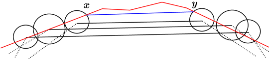
Figure 1: Visualization of the underlying idea of the component $\mathcal{C}$. The black curves are input curves. The red curve $\sigma$ is a solution for $Q(T,\Delta,\ell)$. The black circles are balls $v_{i,a}+B_{\delta_{i}}$ centered at $v_{i,a}$’s. If $\sigma[x,y]$ is matched to a single segment for every input curve, by shortcutting the subcurve $\sigma[x,y]$ to the blue segment, we can get a curve $\sigma^{\prime}$ that is a solution for $Q(T,\Delta,\ell)$. In addition, every segment of $\sigma^{\prime}$ intersects a ball $v_{i,a}+B_{\delta_{i}}$ centered around some input vertex $v_{i,a}$. It means that the intersection between every segment of $\sigma^{\prime}$ and $\mathcal{G}_{1}$ is not empty, which motivates the definition of $(c_{j,1},c_{j,2})$.

2.2 Constraints with respect to a configuration

We describe several constraints that enforce the intuition behind the definition of a configuration. These constraints (or their relaxations) will be verified by our algorithm. Consider a configuration $\Psi_{l}=(\mathcal{P},\mathcal{C},\mathcal{S},\mathcal{A})$ and a candidate curve $\sigma=(w_{1},\ldots,w_{l})$ to be constructed for $\Psi_{l}$. Constraint 1 requires that the cells in $\mathcal{C}$ are close to the corresponding input subcurves. Constraint 2 restricts the locations of the vertices and edges of $\sigma$. Constraint 3 concerns with whether the vertices of $\sigma$ can be matched to the input curves in an order respecting manner within the error bounds.

Constraint 1: For every $i\in[n]$ and every $j\in[l-1]$, if $\pi_{i}^{-1}(j)$ is some non-empty $[a,b]$, then for every vertex $x$ of $c_{j,1}$ and every vertex $y$ of $c_{j,2}$, there exist points $p,q\in xy$ such that $d_{F}(pq,\tau_{i}[v_{i,a},v_{i,b}])\leq\delta_{i}+2\sqrt{d}\varepsilon\delta_{i}$.

Constraint 2:

1. For every $j\in[l]$, if $\mathcal{A}[j]$ is null, then $w_{j}\in s_{j}$; otherwise, $w_{j}\in s_{j}\cap\mathcal{A}[j]$.

2. For every $j\in[l-1]$, $w_{j}x\cap c_{j,1}\not=\emptyset$ for some point $x\in w_{j}w_{j+1}\cap c_{j,2}$.

Constraint 3:

1. For every vertex $x$ of $\mathcal{A}[1]$ and every vertex $y$ of $\mathcal{A}[l]$, both $d(v_{i,1},x)$ and $d(v_{i,m},y)$ are at most $\delta_{i}+2\sqrt{d}\varepsilon\delta_{\max}$ for all $i\in[n]$.

2. Take any index $i\in[n]$. For all $a\in[m-1]$, define $J_{a}=\bigl{\{}j:\pi_{i}(a)<j\leq\pi_{i}(a+1)\,\wedge\,\mathcal{A}[j]\not=\mathrm{null}\bigr{\}}$, i.e., for $j\in J_{a}$, some point(s) in $\tau_{i,a}$ should be matched to $w_{j}$. Constraint 3(b) requires that for all $a\in[m-1]$, if $J_{a}\not=\emptyset$, there exist points $\{p_{j}\in\tau_{i,a}:j\in J_{a}\}$ such that:

   1. for all $j,k\in J_{a}$, if $j<k$, then $p_{j}\leq_{\tau_{i}}p_{k}$;

   2. for every $j\in J_{a}$ and every vertex $x$ of $\mathcal{A}[j]$, $d(p_{j},x)\leq\delta_{i}+2\sqrt{d}\varepsilon\delta_{\max}$.

3. Take any index $j\in[l-1]$ such that $\mathcal{A}[j]=\mathrm{null}$. Note that $j>1$ in order that $\mathcal{A}[j]=\mathrm{null}$. Let $N_{j}=\bigl{\{}i:\exists\,a_{i}\in[m-1]\,\,\text{s.t.}\,\,\pi_{i}(a_{i})<j\leq\pi_{i}(a_{i}+1)\bigr{\}}$, i.e., for $i\in N_{j}$, some point(s) in $\tau_{i,a_{i}}$ should be matched to $w_{j}$. Constraint 3(c) requires that the following conditions are satisfied for all $i\in N_{j}$.

   1. $w_{j}\!\downarrow\!\tau_{i,a_{i}}\in\tau_{i,a_{i}}$ and $d(w_{j},\tau_{i,a_{i}})\leq\delta_{i}+\sqrt{d}\varepsilon\delta_{\max}$.

   2. If $\pi_{i}(a_{i})<j-1\leq\pi_{i}(a_{i}+1)$ and $\mathcal{A}[j-1]=\mathrm{null}$, then $w_{j-1}\!\downarrow\!\tau_{i,a_{i}}\leq_{\tau_{i}}w_{j}\!\downarrow\!\tau_{i,a_{i}}$.

   3. If $\pi_{i}(a_{i})<j-1\leq\pi_{i}(a_{i}+1)$ and $\mathcal{A}[j-1]\not=\mathrm{null}$, then
      $\tau_{i,a_{i}}\cap(\mathcal{A}[j-1]\oplus B_{\delta_{i}+3\sqrt{d}\varepsilon\delta_{i}})\leq_{\tau_{i}}w_{j}\!\downarrow\!\tau_{i,a_{i}}$.

   4. If $\pi_{i}(a_{i})<j+1\leq\pi_{i}(a_{i}+1)$ and $\mathcal{A}[j+1]=\mathrm{null}$, then $w_{j}\!\downarrow\!\tau_{i,a_{i}}\leq_{\tau_{i}}w_{j+1}\!\downarrow\!\tau_{i,a_{i}}$.

   5. If $\pi_{i}(a_{i})<j+1\leq\pi_{i}(a_{i}+1)$ and $\mathcal{A}[j+1]\not=\mathrm{null}$, then
      $w_{j}\!\downarrow\!\tau_{i,a_{i}}\leq_{\tau_{i}}\tau_{i,a_{i}}\cap(\mathcal{A}[j+1]\oplus B_{\delta_{i}+3\sqrt{d}\varepsilon\delta_{i}})$.

Constraints 1–3 are justified by Lemma 1 below. It is proved by snapping the vertices of the solution curve to the discretization; the details are deferred to Appendix A.

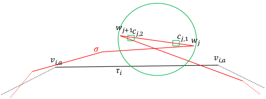
Figure 2: Visualization of the underlying idea of the component $\mathcal{A}$. The black curve is some input curve $\tau_{i}$. The red curve is a solution curve for $Q(T,\Delta,\ell)$ such that every segment intersects a ball centered at some input vertex. Suppose that both $w_{j}$ and $w_{j+1}$ are matched to some points on $\tau_{i,a}$. If $w_{j}\!\downarrow$​ $\tau_{i,a}\geq_{\tau_{i}}w_{j+1}\!\downarrow\!\tau_{i,a}$, the length of $w_{j}w_{j+1}$ must be no more than $2\delta_{i}$. It means that both $w_{j}$ and $w_{j+1}$ can be covered by $B_{9\sqrt{d}\delta_{\max}}+v_{i^{\prime},a^{\prime}}$ for some input vertex $v_{i^{\prime},a^{\prime}}$.

Lemma 1.

If $Q(T,\Delta,\ell)$ has a solution, there exist a configuration $\Psi_{l}$ and a curve $\sigma=(w_{1},\ldots,w_{l})$ for some $l\in[\ell]$ such that constraints 1–3 are satisfied and $d_{F}(\tau_{i},\sigma)\leq\delta_{i}+\sqrt{d}\varepsilon\delta_{\min}$ for $i\in[n]$.

2.3 Forward construction

Given a configuration $\Psi_{l}=(\mathcal{P},\mathcal{C},\mathcal{S},\mathcal{A})$, we check if it satisfies constraint 1, and if so, whether there exists a curve $\sigma$ that satisfies constraints 2 and 3. It is difficult to check constraints 2, 3(c)(ii), and 3(c)(iv) exactly; therefore, we will check some relaxed versions that will be introduced later. We will check constraints 3(b), 3(c)(i), 3(c)(iii), and 3(c)(v) exactly though.

We check constraint 1 as follows. Take any $i\in[n]$ and any $j\in[l-1]$ such that $\pi_{i}^{-1}(j)$ is some non-empty $[a,b]$. Let $x$ and $y$ be any two vertices of $c_{j,1}$ and $c_{j,2}$, respectively. If $xy\cap(v_{i,a}+B_{\delta_{i}+2\sqrt{d}\varepsilon\delta_{i}})$ or $xy\cap(v_{i,b}+B_{\delta_{i}+2\sqrt{d}\varepsilon\delta_{i}})$ is empty, $\Psi_{l}$ does not satisfy constraint 1. Suppose that they are non-empty. Let $p_{1}$ and $p_{2}$ be the points in $xy\cap(v_{i,a}+B_{\delta_{i}+2\sqrt{d}\varepsilon\delta_{i}})$ that are the minimum and maximum with respect to $\leq_{xy}$, respectively. Similarly, let $q_{1}$ and $q_{2}$ be the points in $xy\cap(v_{i,b}+B_{\delta_{i}+2\sqrt{d}\varepsilon\delta_{i}})$ that are the minimum and maximum with respect to $\leq_{xy}$, respectively. We compute $d_{F}(p_{1}q_{2},\tau_{i}[v_{i,a},v_{i,b}])$. If $d_{F}(p_{1}q_{2},\tau_{i}[v_{i,a},v_{i,b}])>\delta_{i}+2\sqrt{d}\varepsilon\delta_{i}$, then $\Psi_{l}$ does not satisfy constraint 1. Otherwise, we repeat the above for all vertices of $c_{j,1}$ and $c_{j,2}$, $j\in[l-1]$, and $i\in[n]$. If the check is passed every time, then $\Psi_{l}$ satisfies constraint 1. For a fixed $i$, the total time needed over all $j\in[l-1]$ is $O(m\log m)$ because $\bigl{|}\bigcup_{j\in[l-1]}\pi_{i}^{-1}(j)\bigr{|}=m$. So the total time over all $i\in[n]$ and all $j\in[l-1]$ is $O(mn\log m)$.

We prove the correctness of this check. There are points $p,q\in xy$ such that $d_{F}(pq,\tau_{i}[v_{i,a},v_{i,b}])\leq\delta_{i}+2\sqrt{d}\varepsilon\delta_{i}$ if and only if there exist points $p\in xy\cap(v_{i,a}+B_{\delta_{i}+2\sqrt{d}\varepsilon\delta_{i}})$ and $q\in xy\cap(v_{i,b}+B_{\delta_{i}+2\sqrt{d}\varepsilon\delta_{i}})$ such that $d_{F}(pq,\tau_{i}[v_{i,a},v_{i,b}])\leq\delta_{i}+2\sqrt{d}\varepsilon\delta_{i}$. Such points $p$ and $q$ lie in $p_{1}p_{2}$ and $q_{1}q_{2}$, respectively. All points in $p_{1}p$ and $qq_{2}$ can be matched to $v_{i,a}$ and $v_{i,b}$, respectively, within the error bound of $\delta_{i}+2\sqrt{d}\varepsilon\delta_{i}$. Hence, $p$ and $q$ exist if and only if $d_{F}(p_{1}q_{2},\tau_{i}[v_{i,a},v_{i,b}])\leq\delta_{i}+2\sqrt{d}\varepsilon\delta_{i}$.

The rest of the forward phase is to inductively compute supersets $\gamma_{1},\ldots,\gamma_{l}$ of the feasible locations of the vertices $w_{1},\ldots,w_{l}$ of $\sigma$ with respect to $\Psi_{l}$. We will see that every $\gamma_{j}$ is a line segment. We need the geometric construct $F(R,S)=\bigl{\{}p\in\mathbb{R}^{d}:\exists\,q\in S\,\,\text{s.t.}\,\,pq\cap R\not=\emptyset\bigr{\}}$, where $R$ and $S$ are two bounded convex polytopes in $\mathbb{R}^{d}$. We can show that $F(R,S)$ is a convex polytope, and it can be constructed by computing a convex hull and a Minkowski sum. In our usage, $|R|$ and $|S|$ are $O(2^{O(d)})$; as a result, $|F(R,S)|=O(2^{O(d)})$ and its construction time is $O(2^{O(d)})$. Refer to Appendix B for details. The inductive computation of $\gamma_{k}$ is as follows. If $\gamma_{j}$ is found empty for any $j\in[l]$, we abort and do not go to the backward phase.

The case of $\boldsymbol{k=1}$. If every vertex of $\mathcal{A}[1]$ is within a distance of $\delta_{i}+2\sqrt{d}\varepsilon\delta_{\max}$ from $v_{i,1}$ for all $i\in[n]$, compute $\gamma_{1}=F(c_{1,1},c_{1,2})\cap s_{1}\cap\mathcal{A}[1]$. Abort otherwise. By constraint 2, $w_{1}\in s_{1}\cap\mathcal{A}[1]$, and $w_{1}x\cap c_{1,1}\not=\emptyset$ for some point $x\in w_{1}w_{2}\cap c_{1,2}$. Therefore, $F(c_{1,1},c_{1,2})\cap s_{1}\cap\mathcal{A}[1]$ represents a relaxed version of constraint 2 on $w_{1}w_{2}$. The processing time of this case is $O(n2^{O(d)})$.

The case of $\boldsymbol{k\in[2,l-1]}$. Suppose that $\gamma_{1},\ldots,\gamma_{k-1}$ have been constructed for some $k\in[2,l-1]$.

Case 1: $\mathcal{A}[k]\not=\mathrm{null}$. Compute $\gamma_{k}=F(c_{k-1,2},\gamma_{k-1})\cap F(c_{k,1},c_{k,2})\cap s_{k}\cap\mathcal{A}[k]$ in $O(2^{(O(d)})$ time.

As before, $w_{k}\in F(c_{k,1},c_{k,2})\cap s_{k}\cap\mathcal{A}[k]$ is a relaxed version of constraint 2 on $w_{k}w_{k+1}$. By constraint 2 again, we must connect $w_{k}$ to $w_{k-1}$, which is in $\gamma_{k-1}$, such that $w_{k-1}w_{k}\cap c_{k-1,2}\not=\emptyset$, implying that $w_{k}\in F(c_{k-1,2},\gamma_{k-1})$. Therefore, $\gamma_{k}=F(c_{k-1,2},\gamma_{k-1})\cap F(c_{k,1},c_{k,2})\cap s_{k}\cap\mathcal{A}[k]$ satisfies a relaxed version of constraint 2.

Let $J^{\prime}_{a}=\{j\in[k]:\pi_{i}(a)<j\leq\pi_{i}(a+1)\,\wedge\,\mathcal{A}[j]\not=\mathrm{null}\}$. To check whether $\gamma_{k}$ satisfies constraint 3(b), we need to check the existence of $\{p_{j}\in\tau_{i,a}:j\in J^{\prime}_{a}\}$ in increasing order of $j$ along $\tau_{i,a}$ that satisfy $d(p_{j},x)\leq\delta_{i}+2\sqrt{d}\varepsilon\delta_{\max}$ for every vertex $x$ of $\mathcal{A}[j]$. Such $p_{j}$’s must lie in the common intersection of $x+B_{\delta_{i}+2\sqrt{d}\varepsilon\delta_{i}}$ over all vertices $x$ of $\mathcal{A}[j]$. For every $j\in J^{\prime}_{a}$, $\tau_{i,a}$ intersects this common intersection in an interval $I_{i,j}$. Let $j_{1}<\ldots<j_{|J^{\prime}_{a}|}$ be the increasing order of indices in $J^{\prime}_{a}$. For $r=|J^{\prime}_{a}|-1,\ldots,1$ in this order, we trim $I_{i,j_{r}}$ to the interval $\{p\in I_{i,j_{r}}:p\leq_{\tau_{i}}\max(I_{i,j_{r+1}})\}$. Afterwards, constraint 3(b) can be satisfied for $i$ if and only if $I_{i,j}\not=\emptyset$ for all $j\in J^{\prime}_{a}$. If the check is passed for every $i\in[n]$ and every $a\in[m-1]$, we accept $\gamma_{k}$; otherwise, we abort. We spend $O(m+l2^{O(d)})$ time over all $a\in[m-1]$ for each $i\in[n]$. The processing time is thus $O(mn2^{O(d)})$.

Case 2: $\mathcal{A}[k]=\mathrm{null}$. To satisfy a relaxed version of constraint 2 for $w_{k-1}w_{k}$ and $w_{k}w_{k+1}$, we require $w_{k}\in F(c_{k-1,2},\gamma_{k-1})\cap F(c_{k,1},c_{k,2})\cap s_{k}$. Recall that $N_{k}=\bigl{\{}i:\exists\,a_{i}\in[m-1]\,\,\text{s.t.}\,\,\pi_{i}(a_{i})<k\leq\pi_{i}(a_{i}+1)\bigr{\}}$. Let $H_{i,a_{i}}$ be the cylinder with axis $\tau_{i,a_{i}}$ and radius $\delta_{i}+\sqrt{d}\varepsilon\delta_{\max}$. To satisfy constraint 3(c)(i), we require $w_{k}\in\bigcap_{i\in N_{k}}H_{i,a_{i}}$. Altogether, we initialize $\gamma_{k}=F(c_{k-1,2},\gamma_{k-1})\cap F(c_{k,1},c_{k,2})\cap s_{k}\cap\bigcap_{i\in N_{k}}H_{i,a_{i}}$. We can compute in $O(2^{O(d)})$ time the clipped segment $F(c_{k-1,2},\gamma_{k-1})\cap F(c_{k,1},c_{k,2})\cap s_{k}$. Then we intersect the clipped segment with each $H_{i,a_{i}}$ in $O(1)$ time. The total initialization time is $O(n+2^{O(d)})$. We may trim $\gamma_{k}$ further as discussed below.

Case 2.1: Suppose that constraint 3(c)(ii) is applicable because $\pi_{i}(a_{i})<k-1\leq\pi_{i}(a_{i}+1)$ and $\mathcal{A}[k-1]=\mathrm{null}$. By constraint 3(c)(i) on $w_{k-1}$, we have $w_{k-1}\in H_{i,a_{i}}$. So $w_{k}$ satisfies constraint 3(c)(ii) if and only if $w_{k}-w_{k-1}$ makes a non-negative inner product with $v_{i,a_{i}+1}-v_{i,a_{i}}$. That is, $w_{k}-w_{k-1}\in\Pi_{i,a_{i}}$, where $\Pi_{i,a_{i}}$ is the closed halfspace containing $v_{i,a_{i}+1}-v_{i,a_{i}}$ such that the bounding hyperplane of $\Pi_{i,a_{i}}$ passes through the origin and is orthogonal to $v_{i,a_{i}+1}-v_{i,a_{i}}$. Since $w_{k-1}w_{k}$ intersects $c_{k-1,2}$, we relax constraint 3(c)(ii) to the restriction that $w_{k}\in\bigcap_{i\in N_{k}^{\prime}}c_{k-1,2}\oplus\Pi_{i,a_{i}}$, where $N^{\prime}_{k}=\bigl{\{}i\in N_{k}:\pi_{i}(a_{i})<k-1\leq\pi_{i}(a_{i}+1)\,\wedge\,\mathcal{A}[k-1]=\mathrm{null}\bigr{\}}$. There is no need to compute $\bigcap_{i\in N^{\prime}_{k}}c_{k-1,2}\oplus\Pi_{i,a_{i}}$ because we can clip $\gamma_{k}$ with each $c_{k-1,2}\oplus\Pi_{i,a_{i}}$ in $O(2^{O(d)})$ time.

Case 2.2: Suppose that constraint 3(c)(iii) is applicable because $\pi_{i}(a_{i})<k-1\leq\pi_{i}(a_{i}+1)$ and $\mathcal{A}[k-1]\not=\mathrm{null}$. We compute in $O(2^{O(d)})$ time the point $p_{i,a_{i}}\in\tau_{i,a_{i}}\cap(\mathcal{A}[k-1]\oplus B_{\delta_{i}+3\sqrt{d}\varepsilon\delta_{i}})$ that is maximum according to $\leq_{\tau_{i}}$. We already require $w_{k}\in H_{i,a_{i}}$. Thus, satisfying constraint 3(c)(iii) is equivalent to requiring $w_{k}\in p_{i,a_{i}}+\Pi_{i,a_{i}}$. The extra restriction in Case 2.2 is thus $w_{k}\in\bigcap_{i\in N^{\prime\prime}_{k}}(p_{i,a_{i}}+\Pi_{i,a_{i}})$, where $N^{\prime\prime}_{k}=\bigl{\{}i\in N_{k}:\pi_{i}(a_{i})<k-1\leq\pi_{i}(a_{i}+1)\,\wedge\,\mathcal{A}[k-1]\not=\mathrm{null}\bigr{\}}$. We do not compute $\bigcap_{i\in N^{\prime\prime}_{k}}(p_{i,a_{i}}+\Pi_{i,a_{i}})$; we clip $\gamma_{k}$ with each $p_{i,a_{i}}+\Pi_{i,a_{i}}$ in $O(1)$ time instead.

Case 2.3: Suppose that $\pi_{i}(a_{i})<k+1\leq\pi_{i}(a_{i}+1)$ and $\mathcal{A}[k+1]=\mathrm{null}$. As in case 2.1 above, constraint 3(c)(iv) for $w_{k}w_{k+1}$ requires $w_{k+1}-w_{k}\in\Pi_{i,a_{i}}$; we relax this requirement to the extra restriction that $w_{k}\in\bigcap_{i\in N^{*}_{k}}c_{k,2}\oplus(-\Pi_{i,a_{i}})$, where $N^{*}_{k}=\bigl{\{}i\in N_{k}:\pi_{i}(a_{i})<k+1\leq\pi_{i}(a_{i}+1)\,\wedge\,\mathcal{A}[k+1]=\mathrm{null}\bigr{\}}$. We can clip $\gamma_{k}$ with each $c_{k,2}\oplus(-\Pi_{i,a_{i}})$ in $O(2^{O(d)})$ time.

Case 2.4: Suppose that $\pi_{i}(a_{i})<k+1\leq\pi_{i}(a_{i}+1)$ and $\mathcal{A}[k+1]\not=\mathrm{null}$. We compute in $O(2^{O(d)})$ time the minimum point $q_{i,a_{i}}$ in $\tau_{i,a_{i}}\cap(\mathcal{A}[k+1]\oplus B_{\delta_{i}+3\sqrt{d}\varepsilon\delta_{i}})$ according to $\leq_{\tau_{i}}$ for all $i\in N_{k}$. As in case 2.2, satisfying constraint 3(c)(v) is equivalent to requiring that $w_{k}\in q_{i,a_{i}}-\Pi_{i,a_{i}}$. So the extra restriction is $w_{k}\in\bigcap_{i\in N^{**}_{k}}(q_{i,a_{i}}-\Pi_{i,a_{i}})$, where $N^{**}_{k}=\bigl{\{}i\in N_{k}:\pi_{i}(a_{i})<k+1\leq\pi_{i}(a_{i}+1)\,\wedge\,\mathcal{A}[k+1]\not=\mathrm{null}\bigr{\}}$. We can clip $\gamma_{k}$ with each $q_{i,a_{i}}-\Pi_{i,a_{i}}$ in $O(1)$ time.

Summary: We list the different definitions of $\gamma_{k}$ for $k\in[2,l-1]$ in the following.

• $\mathcal{A}[k]\not=\mathrm{null}$: Compute $\gamma_{k}=F(c_{k-1,2},\gamma_{k-1})\cap F(c_{k,1},c_{k,2})\cap s_{k}\cap\mathcal{A}[k]$. Check constraint 3(b).

• $\mathcal{A}[k]=\mathrm{null}$: Initialize $\gamma_{k}=F(c_{k-1,2},\gamma_{k-1})\cap F(c_{k,1},c_{k,2})\cap s_{k}\cap\bigcap_{i\in N_{k}}H_{i,a_{i}}$. If $N^{\prime}_{k}\not=\emptyset$, update $\gamma_{k}=\gamma_{k}\cap\bigcap_{i\in N^{\prime}_{k}}c_{k-1,2}\oplus\Pi_{i,a_{i}}$. If $N^{\prime\prime}_{k}\not=\emptyset$, update $\gamma_{k}=\gamma_{k}\cap\bigcap_{i\in N^{\prime\prime}_{k}}(p_{i,a_{i}}+\Pi_{i,a_{i}})$. If $N^{*}_{k}\not=\emptyset$, update $\gamma_{k}=\gamma_{k}\cap\bigcap_{i\in N^{*}_{k}}c_{k,2}\oplus(-\Pi_{i,a_{i}})$. If $N^{**}_{k}\not=\emptyset$, update $\gamma_{k}=\gamma_{k}\cap\bigcap_{i\in N^{**}_{k}}(q_{i,a_{i}}-\Pi_{i,a_{i}})$.

The total processing time for Case 2 is $O(n2^{O(d)})$.

The case of $\boldsymbol{k=l}$. Since $\mathcal{A}[l]\not=\mathrm{null}$, we proceed as in the case of $k\in[2,l-1]$, but we do not need to consider $(c_{l,1},c_{l,2})$. That is, we compute $\gamma_{l}=F(c_{l-1,2},\gamma_{l-1})\cap s_{l}\cap\mathcal{A}[l]$ in $O(2^{O(d)})$ time, and we check constraints 3(a) and 3(b) in $O(mn2^{O(d)})$ time as before.

Lemma 2.

Given a configuration $\Psi_{l}$, the forward construction runs in $O(mn\log m+lmn2^{O(d)})$ time. If $\Psi_{l}$ satisfies constraint 1 and there exists a curve $\sigma=(w_{1},\ldots,w_{l})$ that satisfies constraints 2 and 3 with respect to $\Psi_{l}$, the forward construction produces a sequence of non-empty line segments $(\gamma_{1},\ldots,\gamma_{l})$ such that $w_{j}\in\gamma_{j}$ for all $j\in[l]$.

2.4 Backward extraction

Suppose that the forward construction succeeds with the output $\gamma_{1},\ldots,\gamma_{l}$. The backward extraction works as follows. Set $u_{l}$ to be any point in $\gamma_{l}$. For $j=l-1,\ldots,1$ in this order, set $u_{j}$ to be any point in $F(c_{j,2},u_{j+1})\cap\gamma_{j}$ in $O(2^{O(d)})$ time. Let $\sigma=(u_{1},\ldots,u_{l})$ denote the extraction output.

The extraction succeeds in $O(l2^{O(d)})$ time if $F(c_{j,2},u_{j+1})\cap\gamma_{j}$ is not empty for every $j$. No matter which scenario was applicable in computing $\gamma_{j+1}$ in the forward phase, we always have $\gamma_{j+1}\subseteq F(c_{j,2},\gamma_{j})$. It follows that $u_{j+1}\in F(c_{j,2},\gamma_{j})$, meaning that there exists a point $q\in\gamma_{j}$ such that $qu_{j+1}\cap c_{j,2}\not=\emptyset$. This point $q$ belongs to $F(c_{j,2},u_{j+1})$, which implies that $F(c_{j,2},u_{j+1})\cap\gamma_{j}\not=\emptyset$.

Due to the relaxation of constraint 2 in the forward phase, we cannot ensure that $u_{j}u_{j+1}$ intersects $c_{j,1}$, but we can bound $d(u_{j}u_{j+1},c_{j,1})$ and $d(u_{j}u_{j+1},c_{j,2})$. We can also bound the Fréchet distance between an edge of $\tau_{i}$ and the subcurve of $\sigma$ matched to it according to $\pi_{i}$.

Lemma 3.

For all $j\in[l-1]$, there exist points $p,q\in u_{j}u_{j+1}$ such that $p\leq_{\sigma}q$ and both $d(p,c_{j,1})$ and $d(q,c_{j,2})$ are at most $\sqrt{d}\varepsilon\delta_{\max}$.

Lemma 4.

Take any $i\in[n]$ and any $a\in[m-1]$. Suppose that $[k_{1},k_{2}]=\{j:\pi_{i}(a)<j\leq\pi_{i}(a+1)\}$ is non-empty. There exist points $p,q\in\tau_{i,a}$ such that $d_{F}(pq,\sigma[u_{k_{1}},u_{k_{2}}])\leq\delta_{i}+4\sqrt{d}\varepsilon\delta_{\max}$.

Lemma 5.

For all $i\in[n]$, $d_{F}(\sigma,\tau_{i})\leq\delta_{i}+4\sqrt{d}\epsilon\delta_{\max}$.

Proof.

To prove the lemma, we define a matching $f_{i}$ from $\tau_{i}$ to $\sigma$ as follows. First, we define $f_{i}^{-1}$ at the vertices of $\sigma$. Take any $a\in[m-1]$. If $\{j:\pi_{i}(a)<j\leq\pi_{i}(a+1)\}$ is some non-empty $[k_{1},k_{2}]$, by Lemma 4, there is a Fréchet matching $g_{i,a}$ from $\sigma[u_{k_{1}},u_{k_{2}}]$ to a segment $pq\subseteq\tau_{i,a}$ such that $d_{g_{i,a}}(pq,\sigma[u_{k_{1}},u_{k_{2}}])\leq\delta_{i}+4\sqrt{d}\varepsilon\delta_{\max}$; we define $f_{i}^{-1}(u_{j})=g_{i,a}(u_{j})$ for all $j\in[k_{1},k_{2}]$. Repeating the above for all $a\in[m-1]$ makes $f_{i}^{-1}(u_{j})\leq_{\tau_{i}}f_{i}^{-1}(u_{k})\iff j\leq k$. Moreover, for every $j\in[l]$ and every $x\in f_{i}^{-1}(u_{j})$, $d(u_{j},x)\leq\delta_{i}+4\sqrt{d}\varepsilon\delta_{\max}$. Any unprocessed $u_{j}$ must satisfy $j>\pi_{i}(m)$; therefore, $u_{j}$ should be matched to $v_{i,m}$, and we define $f_{i}^{-1}(u_{j})=\{v_{i,m}\}$.

Next, we define $f_{i}$ at the vertices of $\tau_{i}$. First, define $f_{i}(v_{i,a})=u_{1}$ for all $a\in\pi_{i}^{-1}(0)$. Take any $j\in[l-1]$ such that $\pi_{i}^{-1}(j)$ is some non-empty $[a,b]$. Let $x$ and $y$ be two vertices of $c_{j,1}$ and $c_{j,2}$, respectively. By constraint 1, there exist $pq\subseteq xy$ such that $d_{F}(pq,\tau_{i}[v_{i,a},v_{i,b}])\leq\delta_{i}+2\sqrt{d}\varepsilon\delta_{i}$. Let $h_{i}$ be a Fréchet matching from $\tau_{i}[v_{i,a},v_{i,b}]$ to $pq$.

By Lemma 3, there exist points $p^{\prime},q^{\prime}\in u_{j}u_{j+1}$ such that $p^{\prime}\leq_{\sigma}q^{\prime}$ and both $d(p^{\prime},c_{j,1})$ and $d(q^{\prime},c_{j,2})$ are at most $\sqrt{d}\varepsilon\delta_{\max}$. It follows that $d(x,p^{\prime})\leq 2\sqrt{d}\varepsilon\delta_{\max}$ and $d(y,q^{\prime})\leq 2\sqrt{d}\varepsilon\delta_{\max}$. As $pq\subseteq xy$, we can take the linear interpolation $h$ from the oriented segment $xy$ to the oriented segment $p^{\prime}q^{\prime}$, which ensures that $d(z,h(z))\leq 2\sqrt{d}\varepsilon\delta_{\max}$ for every point $z\in pq$.

For every $c\in\pi_{i}^{-1}(j)$, we define $f_{i}(v_{i,c})=h\circ h_{i}(v_{i,c})$. The Fréchet matching $h_{i}$ and the linear interpolation $h$ guarantee that $f_{i}(v_{i,c})\leq_{\sigma}f_{i}(v_{i,c^{\prime}})\iff c\leq c^{\prime}$. According to the previous discussion, for every $c\in\pi_{i}^{-1}(j)$, $d(v_{i,c},f_{i}(v_{i,c}))\leq\delta_{i}+4\sqrt{d}\varepsilon\delta_{\max}$. Repeating the above for all $j\in[l-1]$ such that $\pi_{i}^{-1}(j)\not=\emptyset$ defines $f_{i}$ at all vertices of $\tau_{i}$.

Thanks to the property of $\pi_{i}$, the definitions of $f_{i}^{-1}$ at the vertices of $\sigma$ and the definitions of $f_{i}$ at the vertices of $\tau_{i}$ do not cause any conflict or order violation along $\sigma$ and $\tau_{i}$.

We have taken care of the vertices of $\sigma$ and $\tau_{i}$. We use linear interpolation to match all other points between $\tau_{i}$ and $\sigma$; it also maintains the distance bound of $\delta_{i}+4\sqrt{d}\varepsilon\delta_{\max}$. ∎

2.5 Accelerating the algorithm

Observe that a configuration only needs to guarantee that the endpoints of the segments $\gamma_{1},\ldots,\gamma_{l}$ can be produced by the components $\mathcal{C}$, $\mathcal{S}$, $\mathcal{A}$, and other linear constraints induced by the input curves. As there are only $2l$ segment endpoints, only $O(l)$ input curves are involved in defining $\gamma_{1},\ldots,\gamma_{l}$. In Appendix D, we show that $5l$ are sufficient.

We do not know which $5l$ input curves to sample, so we enumerate all subsets of $5l$ input curves. For each subset, the number of configurations drops to $O\bigl{(}m^{O(\ell^{2})}\cdot(\ell/\varepsilon)^{O(d\ell)}\bigr{)}$, and the running time of the forward construction reduces to $O(ml\log m+ml^{2}2^{O(d)})$. For each candidate output curve $\sigma$, we need to verify whether $\sigma$ works for the remaining $n-5l$ input curves that are not used for constructing $\sigma$. We check by computing $d_{F}(\sigma,\tau_{i})$ and comparing it with $\delta_{i}+4\sqrt{d}\varepsilon\delta_{\max}$ for all $i\in[n]$. The time needed for this check is $O(lmn\log(ml))$. To go from the error bounds $\delta_{i}+4\sqrt{d}\varepsilon\delta_{\max}$ to $\delta_{i}+\varepsilon\delta_{\max}$, we need to reduce $\varepsilon$ to $\varepsilon/(4\sqrt{d})$ in the definition of ${\mathcal{G}}_{1}$ and ${\mathcal{G}}_{2}$. Finally, we repeat the above for each $l\in[\ell]$ in order to solve $Q(T,\Delta,\ell)$ approximately.

Theorem 1.

Let $T=\{\tau_{1},\ldots,\tau_{n}\}$ be $n$ polygonal curves of $m$ vertices each in $\mathbb{R}^{d}$. Let $\Delta=\{\delta_{1},\ldots,\delta_{n}\}$ be $n$ error thresholds. Let $\ell\leq m$ be a positive integer. Let $\varepsilon$ be a fixed value in $(0,1)$. There is an algorithm that returns a null output or a polygonal curve $\sigma$ of at most $\ell$ vertices such that $d_{F}(\sigma,\tau_{i})\leq\delta_{i}+\varepsilon\delta_{\max}$ for $i\in[n]$. If the output is null, there is no curve $\sigma$ of at most $\ell$ vertices such that $d_{F}(\sigma,\tau_{i})\leq\delta_{i}$ for $i\in[n]$. The running time of the algorithm is $\tilde{O}\bigl{(}n^{O(\ell)}\cdot m^{O(\ell^{2})}\cdot(d\ell/\varepsilon)^{O(d\ell)}\bigr{)}$.

When $n=1$, we can use Theorem 1—the version without picking subsets of $5l$ input curves—to approximately minimize both the error and the output size in curve simplification.

Theorem 2.

Let $\tau$ be a polygonal curve of $m$ vertices in $\mathbb{R}^{d}$. Let $\delta$ be an error threshold. Let $\alpha$ and $\varepsilon$ be some fixed values in $(0,1)$. There is an algorithm that computes a polygonal curve $\sigma$ such that $d_{F}(\sigma,\tau)\leq(1+\varepsilon)\delta$ and $|\sigma|\leq(1+\alpha)\kappa(\tau,\delta)$. The running time is $\tilde{O}\bigl{(}(m^{O(1/\alpha)}\cdot(d/(\alpha\varepsilon))^{O(d/\alpha)}\bigr{)}$.

Proof.

Let $\tau=(v_{1},\ldots,v_{m})$. Compute the smallest $i\in[m]$ such that $Q(\{\tau[v_{1},v_{i+1}]\},\{\delta\},\lceil 1/\alpha\rceil)$ has no solution. We have spent $\tilde{O}\bigl{(}i\cdot m^{O(1/\alpha)}\cdot(d/(\alpha\varepsilon))^{O(d/\alpha)}\bigr{)}$ time so far and obtain a curve $\sigma_{1}$ such that $|\sigma_{1}|\leq 1/\alpha$ and $d_{F}(\sigma_{1},\tau[v_{1},v_{i}])\leq(1+\varepsilon)\delta$. Then we repeat the above for $\tau[v_{i+1},v_{m}]$ to obtain another curve $\sigma_{2}$. In the end, we connect $\sigma_{1},\sigma_{2},\ldots$ to form the output curve $\sigma$. The distance between $v_{i}$ and the last endpoint of $\sigma_{1}$ is at most $(1+\varepsilon)\delta$, and so is the distance between $v_{i+1}$ and the first endpoint of $\sigma_{2}$; therefore, a linear interpolation shows that we can connect $\sigma_{1}$ and $\sigma_{2}$ without violating the $(1+\varepsilon)\delta$ Fréchet distance bound. The same analysis applies to the connections between $\sigma_{2}$ and $\sigma_{3}$ and so on. The greedy process means that we introduce at most one extra edge for every $1/\alpha$ edges in the optimal solution, implying that $|\sigma|\leq(1+\alpha)\kappa(\tau,\delta)$. ∎

3 $\boldsymbol{(k,\ell)}$-median clustering

Take any $\alpha,\beta\in[1,\infty)$ and $\mu\in(0,1)$. An algorithm is an $(\alpha+\varepsilon)$-approximate candidate finder with success probability at least $1-\mu$ if it computes a set $\Sigma$ of curves, each of $\ell$ vertices, and for every subset $S\subseteq T$ that has size $\frac{1}{\beta}|T|$ or more, it holds with probability at least $1-\mu$ that $\Sigma$ contains an $(\alpha+\varepsilon)$-approximate $(1,\ell)$-median of $S$. The following result of Buchin et al. [6] says that a finder can be used for $(k,\ell)$-median clustering. We use $\mathrm{cost}(T,\Sigma)$ to denote $\sum_{\tau_{i}\in T}\min_{\sigma\in\Sigma}d_{F}(\sigma,\tau_{i})$. If $\Sigma$ consists of a single curve $\sigma$, we will just write $\mathrm{cost}(T,\sigma)$ for $\sum_{\tau_{i}\in T}d_{F}(\sigma,\tau_{i})$.

Lemma 6 (Theorem 7.2 [6]).

One can use an $(\alpha+\varepsilon)$-approximate candidate finder $A$ with success probability at least $1-\mu$ to compute a set $\Sigma$ of $k$ curves, each of $\ell$ vertices, such that $\mathrm{cost}(T,\Sigma)\leq(1+\frac{4k^{2}}{\beta-2k})(\alpha+\varepsilon)\cdot\mathrm{OPT}$ with probability at least $1-\mu$, where $\mathrm{OPT}$ is the optimal $(k,\ell)$-median cost for $T$. The running time is $O\bigr{(}T_{A}\cdot C_{A}^{k+1}+n\cdot C_{A}^{k+2}\bigr{)}$, where $T_{A}$ is the running time of $A$ and $C_{A}$ is the number of curves returned by $A$.

We will present a $(1+\varepsilon$)-approximate candidate finder such that $T_{A}$ and $C_{A}$ are $\tilde{O}\bigl{(}(m/\mu)^{O(\ell)}\cdot(d\beta\ell/\varepsilon)^{O((d\ell/\varepsilon)\log(1/\mu))}\bigr{)}$. Using our finder with $\beta=\Theta(k^{2}/\varepsilon)$ and adjusting $\varepsilon$ by a constant factor, Lemma 6 gives a $(1+\varepsilon)$-approximation algorithm for the $(k,\ell)$-median clustering problem.

Our finder makes heavy use of the configurations in Section 2.1. Some notations are needed for the exposition. Let $C(R,l,\alpha)$ be the set of all configurations with respect to a subset $R\subset T$, the target size $l$ of the simplified curve, and the approximation ratio $\alpha\in(0,1)$. There is a given set of error thresholds for $R$ that we do not specify explicitly in order not to clutter the notation. It will be clear from the context what these error thresholds are.

We enhance the finder in [6] to enumerate certain configurations and compute the corresponding curves using the two-phase construction. Algorithm 1 shows this finder. Since we aim for a probabilistic result, we sample a subset $Y\subset T$ of size $\frac{80\beta\ell}{\varepsilon}\ln\frac{80\ell}{\mu}$ and work with the configurations for all subsets of $Y$ of size $\frac{1}{2\beta}|Y|$. This will allow us to capture $\Theta(l)$ input curves that induce almost all configurations necessary. This is formalized in Lemma 7 below.

Lemma 7.

Take any subset $S\subseteq T$ with at least $n/\beta$ curves for any $\beta\geq 1$. Let $\Delta=\{\delta_{1},\ldots,\delta_{|S|}\}$ be a set of error thresholds for $S$ such that $Q(S,\Delta,\ell)$ has a solution. Relabel elements, if necessary, so that $\delta_{1}\leq\ldots\leq\delta_{|S|}$. For $i\in\bigl{[}|S|\bigr{]}$, let $S_{i}=\{\tau_{i},\tau_{i+1},\ldots\}$ and let $\Delta_{i}=\{\delta_{i},\delta_{i+1},\ldots\}$. Take any $\alpha,\varepsilon\in(0,1)$ and any $r\in\bigl{[}\frac{\varepsilon|S|}{5\ell}\bigr{]}$. There exists $\mathcal{H}_{r}\subseteq 2^{S_{r}}$ such that $|\mathcal{H}_{r}|=3l-1$ for some $l\in[\ell]$, every subset in $\mathcal{H}_{r}$ has $\frac{\varepsilon|S|}{5\ell}$ curves, and for every subset $R\subseteq S_{r}$, if $\tau_{r}\in R$ and $R\cap H\not=\emptyset$ for all $H\in\mathcal{H}_{r}$, there exist a configuration $\Psi=(\mathcal{P},\mathcal{C},\mathcal{S},\mathcal{A})\in C(\overline{\mathcal{H}}_{r}\cup R,h,\alpha)$ and a curve $\sigma=(w_{1},\ldots,w_{h})$ for some $h\in[l]$, where $\overline{\mathcal{H}}_{r}=S_{r}\setminus\bigcup_{H\in\mathcal{H}_{r}}H$, that satisfy the following properties.

1. $\Psi$ and $\sigma$ satisfy constraints 1–3 with respect to $\overline{\mathcal{H}}_{r}\cup R$.

2. There exists a configuration in $C(R,h,\alpha)$ that shares the components $\mathcal{C}$, $\mathcal{S}$, and $\mathcal{A}$ with $\Psi$.

Lemma 7 is formulated for different $r\in\bigl{[}\frac{\varepsilon|S|}{5\ell}\bigr{]}$ because the sample of curves in Algorithm 1 will include some curves among $\tau_{1},\ldots,\tau_{\varepsilon|S|/(5\ell)}$ with good probability, but we do not know a priori which ones. By the Chernoff bound, we can sample a small subset $R\subseteq S_{r}$ that satisfies Lemma 7 with high probability. The set $R$ acts like the $\Theta(l)$ curves that induce the components of a configuration in Section 2.5. Indeed, the proof of Lemma 7 in Appendix E uses a similar argument. How should the error thresholds for $R$ be set? In lines 1 and 1, Algorithm 1 computes a 34-approximate $(1,\ell)$-median $c$, with success probability at least $1-\mu/4$, to identify an upper bound $U$ and a lower bound $L$ on the error thresholds. Then, we try all possible sets of integral multiples of $L$ in the range $[L,U]$ in line 1. There are at most $3\varepsilon|S|/5$ curves in $S_{r}\setminus(\overline{\mathcal{H}}_{r}\cup R)$ that Lemma 7(i) says nothing about; the analysis will take care of them separately. The specific values $n/\beta$ and $\frac{\varepsilon|S|}{5\ell}$ are not critical for the proof of Lemma 7. They are chosen to interface with the subsequent analysis of the approximation ratio of Algorithm 1.

Data: $T=\{\tau_{1},...,\tau_{n}\},\,\ell\in\mathbb{Z}_{>0},\,\beta\geq 1,\,\text{and}\;\mu,\varepsilon\in(0,1)$.

Result: A set $\Sigma$ of curves, each of $\ell$ vertices; for every subset $S\subseteq T$ of size $\frac{1}{\beta}|T|$ or more, it holds with probability at least $1-\mu$ that there exists a curve $\sigma\in\Sigma$ such that $\mathrm{cost}(S,\sigma)\leq(1+O(\sqrt{d}\ell\varepsilon))\cdot\text{optimal $(1,\ell)$-median cost of $S$}$.

1 begin

2       $\Sigma\leftarrow\emptyset$;

3       $Y\leftarrow$ a multiset of $\bigl{\lceil}\frac{80\beta\ell}{\varepsilon}\ln\frac{80\ell}{\mu}\bigr{\rceil}$ curves that are uniformly, independently sampled from $T$ with replacement;

4       for each multi-subset $X\subseteq Y$ such that $|X|=|Y|/(2\beta)$ do

5             $c\leftarrow$ $(1,\ell)$-median-34-approximation$(X,\mu/4)$;   /* Algorithm 1 in [6] */

6             $\Sigma\leftarrow\Sigma\cup\{c\}$;

7             $U\leftarrow\frac{10\ell}{\varepsilon^{2}}\mathrm{cost}(X,c)$; $L\leftarrow\frac{\varepsilon\mu}{34|X|}\mathrm{cost}(X,c)$;

8             for each $l\in[\ell]$ and each $h\in[l]$ do

9                   for each possible simple subset $W\subseteq X$ of size at most $3l+2h$ do

10                         for each possible set $\Delta_{W}=\{\delta_{i}:\tau_{i}\in W,\,\delta_{i}=b_{i}L\,\,\text{\emph{for some $b_{i}\in\bigl{[}\lceil U/L\rceil\bigr{]}$}}\}$ do

11                               $\Sigma^{\prime}\leftarrow$ curves produced by the two-phase method on all configurations in $C(W,h,\varepsilon^{2})$ with respect to $\Delta_{W}$; note that the approximation ratio is $\varepsilon^{2}$ instead of $\varepsilon$;

12                               if $h<\ell$ then

13                                     for each $\sigma\in\Sigma^{\prime}$ do

14                                           arbitrarily make $\ell-h$ points on $\sigma$ as extra vertices;

15                                          

16                                     end for

17                                    

18                               end if

19                              $\Sigma\leftarrow\Sigma\cup\Sigma^{\prime}$

20                         end for

21                        

22                   end for

23                  

24             end for

25            

26       end for

27      

28 end

29

Algorithm 1 $(1+\varepsilon)$-approximate candidate-finder

Lemma 7(ii) does not immediately allow us to use $R$ to approximate an optimal $(1,\ell)$-median curve for an arbitrary subset $S\subseteq T$. To produce a candidate curve using the two-phase construction, we need to know the curves in $S$ so that we can apply constraints 1–3 (or their relaxations) in the forward construction. Although we do not know $S$, sampling comes to our rescue. Lemma 8 below shows that a small sample can capture the configurations and the effects of the two-phase construction for almost the entire $S$. We introduce a notation for the output of the forward construction. Given a subset $Z\subseteq T$ and a configuration $\Psi\in C(Z,l,\alpha)$, the forward construction produces $l$ line segments; we use $\gamma_{j}(Z,\Psi)$ to denote the $j$-th output segment for $j\in[l]$.

Lemma 8.

Take any subset $S\subseteq T$ with at least $n/\beta$ curves for any $\beta\geq 1$. Let $\Delta$ be a set of error thresholds for $S$ such that $Q(S,\Delta,\ell)$ has a solution. Assume the notation in Lemma 7. Take any $\alpha,\varepsilon\in(0,1)$, any $r\in\bigl{[}\frac{\varepsilon|S|}{5\ell}\bigr{]}$, and any subset $R\subseteq S_{r}$ such that $\tau_{r}\in R$ and $R\cap H\not=\emptyset$ for all $H\in\mathcal{H}_{r}$. Let $\hat{S}_{r}=\overline{\mathcal{H}}_{r}\cup R$. Let $\Psi=(\mathcal{P},\mathcal{C},\mathcal{S},\mathcal{A})\in C(\hat{S}_{r},h,\alpha)$ for some $h\in[\ell]$ be a configuration that satisfies Lemma 7. There exist $\mathcal{H}_{\Psi}\subseteq 2^{\hat{S}_{r}}$ and a configuration $\Psi^{\prime\prime}=(\mathcal{P}^{\prime\prime},\mathcal{C},\mathcal{S},\mathcal{A})\in C(\overline{\mathcal{H}}_{\Psi}\cup R,h,\alpha)$, where $\overline{\mathcal{H}}_{\Psi}=\hat{S}_{r}\setminus\bigcup_{H\in\mathcal{H}_{\Psi}}H$, such that $|\mathcal{H}_{\Psi}|=2h$, every subset in $\mathcal{H}_{\Psi}$ contains $\frac{\varepsilon|S|}{5\ell}$ curves, and for all subset $R^{\prime}\subseteq\hat{S}_{r}$, if $R^{\prime}\cap H\not=\emptyset$ for all $H\in\mathcal{H}_{\Psi}$, then there exists a configuration $\Psi^{\prime}=(\mathcal{P}^{\prime},\mathcal{C},\mathcal{S},\mathcal{A})\in C(R\cup R^{\prime},h,\alpha)$ that satisfies the following properties.

1. For all $j\in[h]$, $\gamma_{j}(\hat{S}_{r},\Psi)\subseteq\gamma_{j}(R\cup R^{\prime},\Psi^{\prime})\subseteq\gamma_{j}(\overline{\mathcal{H}}_{\Psi}\cup R,\Psi^{\prime\prime})$.

2. The backward extraction using $\{\gamma_{j}(R\cup R^{\prime},\Psi^{\prime}):j\in[h]\}$ produces a curve $\sigma$ such that $d_{F}(\sigma,\tau_{i})\leq\delta_{i}+4\sqrt{d}\alpha\cdot\max\{\delta_{i}:\tau_{i}\in R\cup R^{\prime}\}$ for all $\tau_{i}\in\overline{\mathcal{H}}_{\Psi}\cup R$.

It is an important feature of Lemma 8 that $\Psi$, $\Psi^{\prime}$ and $\Psi^{\prime\prime}$ share the components $\mathcal{C}$, $\mathcal{S}$ and $\mathcal{A}$. Lemma 8 serves the following purpose. The much smaller subsets $R$ and $R^{\prime}$ give line segments $\gamma_{j}(R\cup R^{\prime},\Psi^{\prime})$ that capture the feasible locations of output curve vertices for the much bigger set $\hat{S}_{r}=\overline{\mathcal{H}}_{r}\cup R$. However, this property alone does not say anything about the approximation offered by $\gamma_{j}(R\cup R^{\prime},\Psi^{\prime})$ with respect to the curves in $\hat{S}_{r}$.

The two-phase construction using $\{\gamma_{j}(\overline{\mathcal{H}}_{\Psi}\cup R,\Psi^{\prime\prime}):j\in[h]\}$ will produce an output curve $\sigma$ such that $d_{F}(\sigma,\tau_{i})\leq\delta_{i}+4\sqrt{d}\alpha\cdot\max\{\delta_{i}:\tau_{i}\in\overline{\mathcal{H}}_{\Psi}\cup R\}$ for all $\tau_{i}\in\overline{\mathcal{H}}_{\Psi}\cup R$. One effect of $\Psi^{\prime}$ and $\Psi^{\prime\prime}$ sharing the component $\mathcal{A}$ is that $\max\{\delta_{i}:\tau_{i}\in\overline{\mathcal{H}}_{\Psi}\cup R\}=\max\{\delta_{i}:\tau_{i}\in R\cup R^{\prime}\}$. Recall that the backward extraction can start with any point in $\gamma_{h}(\overline{\mathcal{H}}_{\Psi}\cup R,\Psi^{\prime\prime})$ as the $h$-th output vertex $u_{h}$, and for $j\in[h-1]$, the $j$-th output vertex $u_{j}$ can be any point in $F(c_{j,2},u_{j+1})\cap\gamma_{j}(\overline{\mathcal{H}}_{\Psi}\cup R,\Psi^{\prime\prime})$. We can start with $u_{h}\in\gamma_{h}(R\cup R^{\prime},\Psi^{\prime})\subseteq\gamma_{h}(\overline{\mathcal{H}}_{\Psi}\cup R,\Psi^{\prime\prime})$. For $j\in[h-1]$, since $\mathcal{C}$ is shared by $\Psi^{\prime}$ and $\Psi^{\prime\prime}$, we can pick $u_{j}$ from $F(c_{j,2},u_{j+1})\cap\gamma_{j}(R\cup R^{\prime},\Psi^{\prime})\subseteq F(c_{j,2},u_{j+1})\cap\gamma_{j}(\overline{\mathcal{H}}_{\Psi}\cup R,\Psi^{\prime\prime})$. Therefore, the same approximation guarantees apply to the backward extraction using $\gamma_{j}(R\cup R^{\prime},\Psi^{\prime})$. The proof of Lemma 8 is in Appendix F. The values $n/\beta$ and $\frac{\varepsilon|S|}{5\ell}$ are not critical for the proof of Lemma 8. They are chosen to interface with Lemma 7 and the analysis of the approximation ratio of Algorithm 1.

Lemma 8 allows us to approximate using the small subset $R\cup R^{\prime}$, provided that we know the right error thresholds. Of course, we do not, but we will encounter the right choice in the enumeration of the possible error thresholds in line 1 of Algorithm 1. The capability of Algorithm 1 is analogous to that provided by the approximate candidate finder of Buchin et al. [6]; the major difference being our guarantee that every output curve has $\ell$ vertices, whereas an upper bound of $2\ell-2$ is guaranteed in [6]. We can adapt the analysis in [6] for their approximate candidate finder to show that Algorithm 1 is a $(1+\varepsilon)$-approximate candidate finder. The details are given in Appendix G.

Lemma 9.

For $\varepsilon<1/9$, Algorithm 1 is a $(1+\varepsilon)$-approximate candidate finder with success probability at least $1-\mu$. The algorithm outputs a set $\Sigma$ of curves, each of $\ell$ vertices; for every subset $S\subseteq T$ of size $\frac{1}{\beta}|T|$ or more, it holds with probability at least $1-\mu$ that there exists a curve $\sigma\in\Sigma$ such that $\mathrm{cost}(S,\sigma)\leq(1+\varepsilon)\mathrm{cost}(S,c^{*})$, where $c^{*}$ is the optimal $(1,\ell)$-median of $S$. The running time and output size of Algorithm 1 are $\tilde{O}\bigl{(}m^{O(\ell^{2})}\cdot\mu^{-O(\ell)}\cdot(d\beta\ell/\varepsilon)^{O((d\ell/\varepsilon)\log(1/\mu))}\bigr{)}$.

Combining Lemmas 9 and 6 gives the following result.

Theorem 3.

Let $T$ be a set of $n$ polygonal curves with $m$ vertices each in $\mathbb{R}^{d}$. For any $k,\ell\in\mathbb{Z}_{>0}$ and any $\mu,\varepsilon\in(0,1)$, one can compute a set $\Sigma$ of $k$ curves, each of $\ell$ vertices, and it holds with probability at least $1-\mu$ that $\mathrm{cost}(T,\Sigma)$ is within a factor $1+\varepsilon$ of the optimal $(k,\ell)$-median cost of $T$. The running time is $\tilde{O}\bigl{(}n\cdot m^{O(k\ell^{2})}\cdot\mu^{-O(k\ell)}\cdot(dk\ell/\varepsilon)^{O((dk\ell/\varepsilon)\log(1/\mu))}\bigr{)}$.

Appendix A Proof of Lemma 1

Lemma 1.  If $Q(T,\Delta,\ell)$ has a solution, there exist a configuration $\Psi_{l}$ and a curve $\sigma=(w_{1},\ldots,w_{l})$ for some $l\in[\ell]$ such that constraints 1–3 are satisfied and $d_{F}(\tau_{i},\sigma)\leq\delta_{i}+\sqrt{d}\varepsilon\delta_{\min}$ for $i\in[n]$.

Proof.

Let $\sigma=(u_{1},\ldots,u_{l})$ be a solution curve for $Q(T,\Delta,\ell)$ for some $l\in[\ell]$. For $i\in[n]$, let $g_{i}$ be a Fréchet matching from $\tau_{i}$ to $\sigma$. So $d_{g_{i}}(\tau_{i},\sigma)\leq\delta_{i}$ for all $i\in[n]$.

We require further that for all $j\in[l-1]$, there exist $i\in[n]$ and $a\in[m]$ such that $g_{i}(v_{i,a})\cap u_{j}u_{j+1}\not=\emptyset$. Suppose that this requirement is not met for $u_{j}u_{j+1}$. Then, for every $i\in[n]$, there exists $a_{i}\in[m-1]$ such that $u_{j}u_{j+1}\subseteq g_{i}(\mathrm{int}(\tau_{i,a_{i}}))$. Let $p$ be the maximum of $\{\max(g_{i}(v_{i,a_{i}})):i\in[n]\}$ with respect to $\leq_{\sigma}$. Let $q$ be the minimum of $\{\min(g_{i}(v_{i,a_{i}+1})):i\in[n]\}$ with respect to $\leq_{\sigma}$. Our choice of $p$ and $q$ means that $p\in g_{s}(v_{s,a_{s}})$ and $q\in g_{t}(v_{t,a_{t}+1})$ for some possibly non-distinct $s,t\in[n]$, and $\mathrm{int}(\sigma[p,q])\subseteq g_{i}(\mathrm{int}(\tau_{i,a_{i}}))$ for all $i\in[n]$. We update $\sigma$ by substituting $\sigma[p,q]$ with the edge $pq$, possibly making $p$ and $q$ new vertices of $\sigma$. The number of edges of $\sigma$ is not increased by the replacement; it may actually be reduced. For all $i\in[n]$, we update $g_{i}$ by a linear interpolation along $pq$; since $\mathrm{int}(\sigma[p,q])\subseteq g_{i}(\mathrm{int}(\tau_{i,a_{i}}))$, the replacement of $\sigma[p,q]$ and the linear interpolation ensure that after the update, $g_{i}$ remains a matching and $d_{g_{i}}(\tau_{i},\sigma)\leq\delta_{i}$. Our choice of $p$ and $q$ means that the update does not affect the subset of vertices of $\tau_{i}$ that are matched by any $g_{i}$ to the edges of $\sigma$ other than $pq$. The update also ensures that $pq$ will not trigger another shortcutting, and $pq$ will not be shortened by other shortcuttings. If necessary, we repeat the above to convert $\sigma$ to $(u^{\prime}_{1},u^{\prime}_{2},\ldots)$ such that for every edge $u^{\prime}_{j}u^{\prime}_{j+1}$ there exist $i\in[n]$ and $a\in[m]$ such that $g_{i}(v_{i,a})\cap u^{\prime}_{j}u^{\prime}_{j+1}\not=\emptyset$.

The modified $\sigma$ may have fewer vertices; if so, we decrease the value of $l$ to the current number of vertices in $\sigma$. We use $(u^{\prime}_{1},u^{\prime}_{2},\ldots,u^{\prime}_{l})$ to denote the modified $\sigma$. Let $\min=\mathrm{argmin}_{i\in[n]}\delta_{i}$. Next, we snap the vertices of $\sigma$ to segments in the set $\cal L$. Since $d_{g_{\min}}(\sigma,\tau_{\min})\leq\delta_{\min}$, $\sigma$ lies inside $\tau_{\min}\oplus B_{\delta_{\min}}$, which implies that every vertex $u^{\prime}_{j}$ of $\sigma$ is within a distance of $\sqrt{d}\varepsilon\delta_{\min}$ from the nearest segment $s_{j}$ in $\cal L$. We modify $\sigma$ by moving $u^{\prime}_{j}$ to its nearest point $w_{j}\in s_{j}$ for every $j\in[l]$. For every $i\in[n]$, we update $g_{i}$ using the linear interpolations between $u^{\prime}_{j}u^{\prime}_{j+1}$ and $w_{j}w_{j+1}$ for all $j\in[l-1]$. Consequently, $\sigma=(w_{1},\ldots,w_{l})$ and $d_{g_{i}}(\tau_{i},\sigma)\leq\delta_{i}+\sqrt{d}\varepsilon\delta_{\min}$ for $i\in[n]$. This establishes the second half of the lemma. Notice that this updating of the $g_{i}$’s preserves the property that for all $j\in[l-1]$, there exist $i\in[n]$ and $a\in[m]$ such that $g_{i}(v_{i,a})\cap w_{j}w_{j+1}\not=\emptyset$.

We construct a configuration $\Psi_{l}$ that satisfies constraints 1–3 together with $\sigma$.

For every $i\in[n]$ and every $a\in[m]$, if $w_{1}\in g_{i}(v_{i,a})$, we define $\pi_{i}(a)=0$; otherwise, let $j\in[l-1]$ be the smallest index such that $g_{i}(v_{i,a})\cap w_{j}w_{j+1}\not=\emptyset$ and we define $\pi_{i}(a)=j$. This induces an $n$-tuple $\mathcal{P}=(\pi_{i})_{i\in[n]}$ of the partitions of the vertices of $\tau_{1},\ldots,\tau_{n}$ such that for all $i\in[n]$, $\pi_{i}(1)=0$ and if $a\leq b$, then $\pi_{i}(a)\leq\pi_{i}(b)$.

Next, we define $\mathcal{C}$ as follows. Take any $j\in[l-1]$. Let $x_{j}$ and $y_{j}$ be the minimum and maximum points in $\bigcup_{i\in[n]}\bigcup_{a\in[m]}g_{i}(v_{i,a})\cap w_{j}w_{j+1}$ with respect to $\leq_{\sigma}$, respectively. Note that $\bigcup_{i\in[n]}\bigcup_{a\in[m]}g_{i}(v_{i,a})\cap w_{j}w_{j+1}$ is non-empty because there exist $i\in[n]$ and $a\in[m]$ such that $g_{i}(v_{i,a})\cap w_{j}w_{j+1}\not=\emptyset$. By definition, $x_{j}\leq_{\sigma}y_{j}$. There exists $i\in[n]$ such that $x_{j}$ is within a distance of $\delta_{i}+\sqrt{d}\varepsilon\delta_{\min}$ from a vertex of $\tau_{i}$. We can make the same conclusion about $y_{j}$. It follows that $x_{j}$ and $y_{j}$ belong to cells in ${\mathcal{G}}_{1}$. Choose $c_{j,1}$ and $c_{j,2}$ to be any cells in ${\mathcal{G}}_{1}$ that contain $x_{j}$ and $y_{j}$, respectively. This gives the $(l-1)$-tuple $\mathcal{C}=((c_{j,1},c_{j,2}))_{j\in[l-1]}$.

The components $\mathcal{S}$ and $\mathcal{A}$ of $\Psi_{l}$ are defined as follows. By construction, we know that $w_{j}$ lies on some segment $s_{j}\in\mathcal{L}$. We simply set $\mathcal{S}=(s_{j})_{j\in[l]}$. For every $j\in[l]$, if $w_{j}$ lies in some grid cell in ${\mathcal{G}}_{2}$, set $\mathcal{A}[j]$ to be that cell; otherwise, set $\mathcal{A}[j]$ to be null.

We verify constraint 1. Recall the definitions of $x_{j}$ and $y_{j}$ in defining $(c_{j,1},c_{j,2})$ for every $j\in[l-1]$. Suppose that $\pi_{i}^{-1}(j)$ is some non-empty $[a,b]$. It means that $g_{i}(\tau_{i}[v_{i,a},v_{i,b}])\subseteq x_{j}y_{j}\subseteq w_{j}w_{j+1}$. Let $x$ and $y$ be any vertices of $c_{j,1}$ and $c_{j,2}$, respectively. Therefore, both $d(x,x_{j})$ and $d(y,y_{j})$ are at most $\sqrt{d}\varepsilon\delta_{i}$. Let $h$ be the linear interpolation from the oriented segment $x_{j}y_{j}$ to the oriented segment $xy$. For any point $z\in\tau_{i}[v_{i,a},v_{i,b}]$, $d(z,h\circ g_{i}(z))\leq d_{g_{i}}(\tau_{i},\sigma)+\sqrt{d}\varepsilon\delta_{i}\leq\delta_{i}+2\sqrt{d}\varepsilon\delta_{i}$. It follows that $h\circ g_{i}$ is a matching from $\tau_{i}[v_{i,a},v_{i,b}]$ to some segment $pq\subseteq xy$ such that $d_{h\circ g_{i}}(\tau_{i}[v_{i,a},v_{i,b}],pq)\leq\delta_{i}+2\sqrt{d}\varepsilon\delta_{i}$. This proves that constraint 1 is satisfied.

Constraint 2 is clearly satisfied by construction.

We verify constraint 3(a) as follows. Recall that $d_{g_{i}}(\tau_{i},\sigma)\leq\delta_{i}+\sqrt{d}\varepsilon\delta_{\min}$ for $i\in[n]$. Since the cell $\mathcal{A}[1]$ has side length $\varepsilon\delta_{\max}$, for every vertex $x$ of $\mathcal{A}[1]$, we have $d(v_{i,1},x)\leq d(v_{i,1},w_{1})+\sqrt{d}\varepsilon\delta_{\max}\leq\delta_{i}+2\sqrt{d}\varepsilon\delta_{\max}$. The same analysis applies to $d(v_{i,m},y)$ for every vertex $y$ of $\mathcal{A}[l]$. This establishes constraint 3(a).

Consider constraint 3(b). The set $J_{a}=\bigr{\{}j:\pi_{i}(a)<j\leq\pi_{i}(a+1)\,\wedge\,\mathcal{A}[j]\not=\mathrm{null}\bigr{\}}$ contains the indices of the vertices $w_{j}$’s with non-null $\mathcal{A}[j]$’s such that $g_{i}^{-1}(w_{j})\cap\tau_{i,a}\not=\emptyset$. For all $j\in J_{a}$, pick any point in $g_{i}^{-1}(w_{j})\cap\tau_{i,a}$ to be $p_{j}$. Then, constraint 3(b)(i) follows from the fact that $g_{i}$ is a matching. Constraint 3(b)(ii) follows from the inequalities $d(w_{j},p_{j})\leq d_{g_{i}}(\tau_{i},\sigma)\leq\delta_{i}+\sqrt{d}\varepsilon\delta_{\min}$ and the $\sqrt{d}\varepsilon\delta_{\max}$ bound on the distance from $w_{j}$ to any vertex of the cell $\mathcal{A}[j]$ that contains $w_{j}$.

Consider constraint 3(c). Take any index $j\in[l-1]$ such that $\mathcal{A}[j]=\mathrm{null}$. Recall that $N_{j}=\bigl{\{}i:\exists\,a_{i}\in[m-1]\,\,\text{s.t.}\,\,\pi_{i}(a_{i})<j\leq\pi_{i}(a_{i}+1)\bigr{\}}$. We need to show that constraints 3(c)(i)–(v) are satisfied for all $i\in N_{j}$ whenever they are applicable.

Since $\pi_{i}(a_{i})<j\leq\pi_{i}(a_{i}+1)$, $g_{i}^{-1}$ matches $w_{j}$ to point(s) in $\tau_{i,a_{i}}$ within a distance of $\delta_{i}+\sqrt{d}\varepsilon\delta_{\min}$. It shows that $d(w_{j},\tau_{i,a_{i}})\leq\delta_{i}+\sqrt{d}\varepsilon\delta_{\min}$. The reason why we set $\mathcal{A}[j]$ to be null is that $w_{j}$ lies outside all cells in ${\mathcal{G}}_{2}$. It implies that both $d(v_{i,a_{i}},w_{j})$ and $d(v_{i,a_{i}+1},w_{j})$ are greater than $9\sqrt{d}\delta_{\max}$. Under these circumstances, the condition $w_{j}\!\downarrow\!\tau_{i,a_{i}}\in\tau_{i,a_{i}}$ must hold as it is the only way for $w_{j}$ to be matched to point(s) in $\tau_{i,a_{i}}$ within a distance of $\delta_{i}+\sqrt{d}\varepsilon\delta_{\min}$. So constraint 3(c)(i) is satisfied.

Before we verify constraints 3(c)(ii) and (iii), we claim that $d(w_{j-1},w_{j})\geq 7\sqrt{d}\delta_{\max}$. Take any $r\in[n]$ and any $a\in[m]$ such that $g_{r}(v_{r,a})\cap w_{j-1}w_{j}\not=\emptyset$. If $d(w_{j-1},w_{j})<7\sqrt{d}\delta_{\max}$, then $d(v_{r,a},w_{j})\leq 8\sqrt{d}\delta_{\max}+\sqrt{d}\varepsilon\delta_{\min}$, which implies that $w_{j}$ lies in a grid cell in $G(v_{r,a}+B_{9\sqrt{d}\delta_{\max}},\varepsilon\delta_{\max})\subseteq{\mathcal{G}}_{2}$. But this is a contradiction to the fact that $\mathcal{A}[j]=\mathrm{null}$. This proves the claim.

Suppose that $\pi_{i}(a_{i})<j-1\leq\pi_{i}(a_{i}+1)$ and $\mathcal{A}[j-1]=\mathrm{null}$. So $g_{i}^{-1}$ matches both $w_{j-1}$ and $w_{j}$ to point(s) in $\tau_{i,a_{i}}$. As argued previously for $w_{j}$, we must have $w_{j-1}\!\downarrow\!\tau_{i,a_{i}}\in\tau_{i,a_{i}}$. The angle $\angle(v_{i,a_{i}+1}-v_{i,a_{i}},w_{j}-w_{j-1})$ is either at most $\pi/2$ or greater than $\pi/2$. In the first case, $w_{j-1}\!\downarrow\!\tau_{i,a_{i}}\leq_{\tau_{i}}w_{j}\!\downarrow\!\tau_{i,a_{i}}$, so constraint 3(c)(ii) is satisfied. In the latter case, $d(w_{j},g_{i}^{-1}(w_{j})\cap\tau_{i,a_{i}})\geq d(w_{j-1},w_{j})-\max\{d(w_{j-1},x):x\in g_{i}^{-1}(w_{j-1})\}\geq 7\sqrt{d}\delta_{\max}-\delta_{i}-\sqrt{d}\varepsilon\delta_{\min}>\delta_{i}+\sqrt{d}\varepsilon\delta_{\min}$, a contradiction.

Suppose that $\pi_{i}(a_{i})<j-1\leq\pi_{i}(a_{i}+1)$ and $\mathcal{A}[j-1]\not=\mathrm{null}$. Since $d(w_{j-1},w_{j})\geq 7\sqrt{d}\delta_{\max}$, the distance from $w_{j}\!\downarrow\!\tau_{i,a_{i}}$ to the boundary of $\mathcal{A}[j-1]\oplus B_{\delta_{i}+3\sqrt{d}\varepsilon\delta_{i}}$ is at least $5\sqrt{d}\delta_{\max}-5\sqrt{d}\varepsilon\delta_{i}\geq 0$. Therefore, $w_{j}\!\downarrow\!\tau_{i,a_{i}}$ does not lie inside $\mathcal{A}[j-1]\oplus B_{\delta_{i}+3\sqrt{d}\varepsilon\delta_{i}}$. Since $\max\{d(w_{j},x):x\in g_{i}^{-1}(w_{j})\}$ is at most $\delta_{i}+\sqrt{d}\varepsilon\delta_{\min}$, $g_{i}^{-1}(w_{j})$ does not overlap with $\mathcal{A}[j-1]\oplus B_{\delta_{i}+3\sqrt{d}\varepsilon\delta_{i}}$. Similarly, we have $g_{i}^{-1}(w_{j-1})\subset\mathcal{A}[j-1]\oplus B_{\delta_{i}+3\sqrt{d}\varepsilon\delta_{i}}$. It follows that the ordering of $g_{i}^{-1}(w_{j-1})$ and $g_{i}^{-1}(w_{j})$ along $\tau_{i}$ is the same as that of $g_{i}^{-1}(w_{j-1})$ and $w_{j}\!\downarrow\!\tau_{i,a_{i}}$. Hence, $\tau_{i,a_{i}}\cap(\mathcal{A}[j-1]\oplus B_{\delta_{i}+3\sqrt{d}\varepsilon\delta_{i}})\leq_{\tau_{i}}w_{j}\!\downarrow\!\tau_{i,a_{i}}$. So constraint 3(c)(iii) is satisfied.

We can similarly show that constraint 3(c)(iv) and (v) are satisfied if applicable. ∎

Appendix B A geometric construct

Let $R$ and $S$ be two non-empty, bounded convex polytopes. Recall that $F(R,S)=\{p\in\mathbb{R}^{d}:\exists\,q\in S\,\,\text{s.t.}\,\,pq\cap R\not=\emptyset\}$. Let $\beta_{1},\beta_{2},...,\beta_{|R|}$ be the vertices of $R$. Let $\phi_{1},\phi_{2},...,\phi_{|S|}$ be the vertices of $S$. Let $\psi_{ij}$ be the vector $\beta_{i}-\phi_{j}$ for all $i\in[|R|]$ and $j\in[|S|]$. We prove that $F(R,S)=R\oplus\psi_{RS}$, where $\psi_{RS}$ denotes the set of conical combinations of $\bigl{\{}\psi_{ij}:i\in[|R|],\,j\in[|S|]\bigr{\}}$, i.e., $\sum_{i,j}x_{ij}\psi_{ij}$ for some non-negative $x_{ij}$’s.

Lemma 10.

$F(R,S)=R\oplus\psi_{RS}$.

Proof.

First, we prove that any point $p\in F(R,S)$ can be written as $r+\psi$ for some point $r\in R$ and some conical combination $\psi\in\psi_{RS}$. If $p\in R$, this property is trivially true as we can take $\psi=0$. Suppose that $p\not\in R$. According to the definition of $F(R,S)$, we can find a point $s\in S$ such that the line segment $ps$ intersects $R$. Let $r$ be a point in $ps\cap R$. We have $p=r+\lambda(r-s)$ for some non-negative $\lambda$. Observe that $r\not=s$; otherwise, $p=r\in R$, contradicting the assumption that $p\not\in R$.

We show that $r-s\in\psi_{RS}$. Given that $r\in R$ and $s\in S$, we have $r=\sum_{i=1}^{|R|}a_{i}\beta_{i}$ and $s=\sum_{j=1}^{|S|}b_{j}\phi_{j}$ for some $a_{i},b_{j}\geq 0$ such that $\sum_{i}a_{i}=\sum_{j}b_{j}=1$. To determine whether $r-s\in\psi_{RS}$, we need to verify whether we can find non-negative coefficients $x_{ij}$’s such that $r-s=\sum_{i,j}x_{ij}\psi_{ij}$. We have

$$r-s=\sum_{1\leq i\leq|R|}a_{i}\beta_{i}-\sum_{1\leq j\leq|S|}b_{j}\phi_{j}.$$

By expanding $\sum_{i,j}x_{ij}\psi_{ij}$ we get

$$\sum_{i,j}x_{ij}\psi_{ij}$$

$$= \sum_{i,j}x_{i,j}(\beta_{i}-\phi_{j})$$

$$= \sum_{1\leq i\leq|R|}\Bigl{(}\sum_{1\leq j\leq|S|}x_{ij}\Bigr{)}\beta_{i}-\sum_{1\leq j\leq|S|}\Bigl{(}\sum_{1\leq i\leq|R|}x_{i,j}\Bigr{)}\phi_{j}$$

By comparing terms, we obtain the following linear system.

$x_{i,1}+x_{i,2}+...+x_{i,|S|}=a_{i}$,		$\forall\,1\leq i\leq|R|$,
$x_{1,j}+x_{2,j}+...+x_{|R|,j}=b_{j}$,		$\forall\,1\leq j\leq|S|$,
$x_{ij}\geq 0$,		$\forall\,1\leq i\leq|R|,\,\forall\,1\leq j\leq|S|$.

According to Farkas’ Lemma [10], there exists a vector $x\geq 0$ that satisfies a linear system $Ax=e$ if and only if $ye\geq 0$ for each row vector $y$ such that $yA\geq 0$. In our case, $e$ is the column vector $(a_{1},\ldots,a_{|R|},b_{1},\ldots,b_{|S|})^{t}$, $x$ is the column vector $(x_{1,1},\ldots,x_{1,|S|},\ldots)^{t}$, and $A$ is a $(|R|+|S|)\times(|R||S|)$ matrix. For $0\leq k\leq|R||S|-1$, in the $(k+1)$-th column of $A$, the $(\lfloor k/|R|\rfloor+1)$-th and the $(|R|+1+k~{}\mathrm{mod}~{}|S|)$-th entries are equal to 1, and all other entries are zero. Thus, given a row vector $y=(y_{1},y_{2},...,y_{|R|+|S|})$, it satisfies $yA\geq 0$ if and only if

$$y_{i}+y_{|R|+j}\geq 0,\quad\forall\,1\leq i\leq|R|,\,\forall\,1\leq j\leq|S|.$$

Next, we prove that $ye\geq 0$ if $yA\geq 0$. Expanding $ye$ we get:

$$ye=a_{1}y_{1}+a_{2}y_{2}+...+b_{1}y_{|R|+1}+...+b_{|S|}y_{|R|+|S|}.$$

Without loss of generality, assume that $a_{i^{\prime}}$ is the smallest element among $a_{i}$’s and $b_{j}$’s. Let $k=\min\{i^{\prime},|S|\}$. Then,

$$ye = a_{i^{\prime}}(y_{i^{\prime}}+y_{|R|+k})+\Lambda,\quad\text{where}$$

$$\Lambda = a_{1}y_{1}+...+a_{i^{\prime}-1}y_{i^{\prime}-1}+a_{i^{\prime}+1}y_{i^{\prime}+1}+...+a_{|R|}y_{|R|}+$$

$$b_{1}y_{|R|+1}+...+(b_{k}-a_{i^{\prime}})y_{|R|+k}+...+b_{|S|}y_{|R|+|S|}.$$

Note that $b_{k}-a_{i^{\prime}}\geq 0$. Both $(\sum_{i}a_{i})-a_{i^{\prime}}$ and $(\sum_{j}b_{j})-a_{i^{\prime}}$ are equal to $1-a_{i^{\prime}}$ as $\sum_{i}a_{i}=\sum_{j}b_{j}=1$. We repeat the above to pair another $y_{i}$ and $y_{|R|+j}$. Since the sums of the coefficients decrease by the same amount for the $a_{i}$’s and $b_{j}$’s, there must be nothing left by the repeated pairing in the end. That is, $\Lambda=0$ in the end. As a result, $ye$ can be written as a sum of terms like $y_{i}+y_{|R|+j}$ with non-negative coefficients. Therefore, $ye\geq 0$, and $Ax=e$ has a feasible solution. This shows that $F(R,S)\subseteq R\oplus\psi_{RS}$.

Next, we prove that $R\oplus\psi_{RS}\subseteq F(R,S)$. Consider a point $r+\lambda\sum_{i,j}x_{ij}\psi_{ij}$, where $r\in R$, $\lambda$ is a non-negative real number, and $x_{ij}$’s are non-negative coefficients. If $\sum_{i,j}x_{ij}=0$, then $x_{ij}=0$ for all $i$ and $j$, and the point is just $r$. One can always draw a line through $r$ that intersects $S$, which shows that $r\in F(R,S)$. Suppose that $\sum_{i,j}x_{ij}>0$. Without loss of generality, we assume that $\sum_{i,j}x_{ij}=1$ because, if necessary, $\lambda\sum_{i,j}x_{ij}\psi_{ij}$ can be written as $\lambda\bigl{(}\sum_{i,j}x_{ij}\bigr{)}\cdot\sum_{i,j}\bigl{(}\frac{x_{ij}}{\sum_{i,j}x_{ij}}\bigr{)}\psi_{ij}$.

By expanding $\sum_{i,j}x_{ij}\psi_{ij}$ we get

$$\sum_{i,j}x_{ij}\psi_{ij}=\sum_{1\leq i\leq|R|}\Bigl{(}\sum_{1\leq j\leq|S|}x_{ij}\Bigr{)}\beta_{i}-\sum_{1\leq j\leq|S|}\Bigl{(}\sum_{1\leq i\leq|R|}x_{i,j}\Bigr{)}\phi_{j}.$$

Since $r\in R$, we can write it as $\sum_{i=1}^{|R|}a_{i}\beta_{i}$, where $a_{i}\geq 0$ and $\sum_{i=1}^{|R|}a_{i}=1$. We define

$$a_{i}^{\prime}=\frac{1}{1+\lambda}\left(a_{i}+\lambda\sum_{1\leq j\leq|S|}x_{ij}\right),\quad\quad b^{\prime}_{j}=\sum_{i=1}^{|R|}x_{ij},\quad\quad r^{\prime}=\sum_{i=1}^{|R|}a_{i}^{\prime}\beta_{i},\quad\quad s=\sum_{j=1}^{|S|}b^{\prime}_{j}\phi_{j}.$$

Clearly, $a^{\prime}_{i}$ and $b^{\prime}_{j}$ are non-negative for all $i$ and $j$. Since $\sum_{i}a_{i}=\sum_{i,j}x_{ij}=1$, we have $\sum_{i}a^{\prime}=\frac{1}{1+\lambda}\sum_{i}a_{i}+\frac{\lambda}{1+\lambda}\sum_{i,j}x_{ij}=1$. Also, $\sum_{j}b^{\prime}_{j}=\sum_{i,j}x_{ij}=1$. Therefore, $r^{\prime}$ and $s$ are points in $R$ and $S$, respectively. The point $r+\lambda\sum_{i,j}x_{ij}\psi_{ij}$ is equal to $r^{\prime}+\lambda(r^{\prime}-s)$. Hence, $r+\lambda\sum_{i,j}x_{ij}\psi_{ij}\in F(R,S)$. ∎

Notice that $F(R,S)$ is unbounded. In fact, if $R\cap S\not=\emptyset$, then $F(R,S)=\mathbb{R}^{d}$. The Minkowski sum of $R$ and $\psi_{RS}$ has complexity proportional to the product of their complexities, and so is the construction time of the Minkowski sum. There are at most $|R||S|$ directions in $\{\psi_{ij}\}$. Computing $\psi_{RS}$ boils down to a convex hull computation in $\mathbb{R}^{d-1}$ which has $O\bigl{(}(|R||S|)^{\lfloor(d-1)/2\rfloor}\bigr{)}$ complexity and can be constructed in $O\bigl{(}(|R||S|)^{\lfloor(d-1)/2\rfloor}+|R||S|\log(|R||S|)\bigr{)}$ time.

Lemma 11.

The complexity of $F(R,S)$ is $O(|R|^{1+\lfloor(d-1)/2\rfloor}|S|^{\lfloor(d-1)/2\rfloor})$. The construction time of $F(R,S)$ is $O\bigl{(}|R|^{1+\lfloor(d-1)/2\rfloor}|S|^{\lfloor(d-1)/2\rfloor}+|R||S|\log(|R||S|)\bigr{)}$.

Appendix C Proof of Lemmas 3 and 4

We restate Lemma 3 and give its proof.

Lemma 3  For all $j\in[l-1]$, there exist points $p,q\in u_{j}u_{j+1}$ such that $p\leq_{\sigma}q$ and both $d(p,c_{j,1})$ and $d(q,c_{j,2})$ are at most $\sqrt{d}\varepsilon\delta_{\max}$.

Proof.

We enforce that $u_{j+1}\in\gamma_{j+1}$ and $u_{j}\in F(c_{j,2},u_{j+1})\cap\gamma_{j}$ in the backward extraction. It follows that $u_{j}\in\gamma_{j}$ and $u_{j}u_{j+1}\cap c_{j,2}\not=\emptyset$. Take any point $q\in u_{j}u_{j+1}\cap c_{j,2}$. The forward phase ensures that $\gamma_{j}\subseteq F(c_{j,1},c_{j,2})$, so there is a point $y\in c_{j,2}$ such that $yu_{j}\cap c_{j,1}\not=\emptyset$. As $q$ and $y$ belong to $c_{j,2}$, $d(q,y)\leq\sqrt{d}\varepsilon\delta_{\max}$. Take any point $x\in yu_{j}\cap c_{j,1}$. By a linear interpolation between $yu_{j}$ and $qu_{j}$, $x$ is mapped to a point $p\in qu_{j}$ such that $d(p,x)\leq d(q,y)\leq\sqrt{d}\varepsilon\delta_{\max}$. Clearly, $p\leq_{\sigma}q$. ∎

We restate Lemma 4 and give its proof.

Lemma 4.  Take any $i\in[n]$ and any $a\in[m-1]$. Suppose that $[k_{1},k_{2}]=\{j:\pi_{i}(a)<j\leq\pi_{i}(a+1)\}$ is non-empty. There exist points $p,q\in\tau_{i,a}$ such that $d_{F}(pq,\sigma[u_{k_{1}},u_{k_{2}}])\leq\delta_{i}+4\sqrt{d}\varepsilon\delta_{\max}$.

Proof.

To prove the lemma, we specify a matching $g$ from $\sigma[u_{k_{1}},u_{k_{2}}]$ to a segment in $\tau_{i,a}$. The idea is to define $g$ on the vertices $u_{k}$ for $k\in[k_{1},k_{2}]$ first and then use linear interpolation to extend $g$ to other points in $\sigma[u_{k_{1}},u_{k_{2}}]$.

Let $J_{a}=\{j:\pi_{i}(a)<j\leq\pi_{i}(a+1)\,\wedge\,\mathcal{A}[j]\not=\mathrm{null}\}$. By constraint 3(b), there exist points $\{p_{j}\in\tau_{i,a}:j\in J_{a}\}$ such that these $p_{j}$’s appear in order along $\tau_{i,a}$, and every $p_{j}$ is within a distance of $\delta_{i}+2\sqrt{d}\varepsilon\delta_{\max}$ from every vertex of $\mathcal{A}[j]$. We first define $g(u_{k})$ for $k\in[k_{1},k_{2}]$ inductively. Consider the base case of $u_{k_{1}}$. If $\mathcal{A}[k_{1}]\not=\mathrm{null}$, let $g(u_{k_{1}})=p_{1}$; otherwise, let $g(u_{k_{1}})=u_{k_{1}}\!\downarrow\!\tau_{i,a}$ which lies on $\tau_{i,a}$ by constraint 3(c)(i). In general, take any $k\in[k_{1}+1,k_{2}]$. If $\mathcal{A}[k]\not=\mathrm{null}$, define $g(u_{k})$ to be the maximum of $g(u_{k-1})$ and $p_{k}$ according to $\leq_{\tau_{i}}$. If $\mathcal{A}[k]=\mathrm{null}$, define $g(u_{k})$ to be the maximum of $g(u_{k-1})$ and $u_{k}\!\downarrow\!\tau_{i,a}$ according to $\leq_{\tau_{i}}$.

The above definition of $g(u_{k})$ automatically guarantees that $g(u_{k-1})\leq_{\tau_{i}}g(u_{k})$ for $k\in[k_{1}+1,k_{2}]$. We need to bound the distance between $u_{k}$ and $g(u_{k})$. For every $k\in[k_{1},k_{2}]$, if $\mathcal{A}[k]\not=\mathrm{null}$, let $y_{k}=p_{k}$; otherwise, let $y_{k}=u_{k}\!\downarrow\!\tau_{i,a}$.

We first prove a claim that for all $k\in[k_{1}+1,k_{2}]$, $y_{k-1}\leq_{\tau_{i}}y_{k}$ or $d(y_{k-1},y_{k})\leq\sqrt{d}\varepsilon\delta_{\max}/l$. Suppose that $\mathcal{A}[k-1]\not=\mathrm{null}$. So $y_{k-1}=p_{k-1}$. If $\mathcal{A}[k]\not=\mathrm{null}$, then $y_{k}=p_{k}$ and constraint 3(b)(ii) ensures that $y_{k-1}\leq_{\tau_{i}}y_{k}$. If $\mathcal{A}[k]=\mathrm{null}$, then $y_{k}=u_{k}\!\downarrow\!\tau_{i,a}$. By constraint 3(b)(ii), $y_{k-1}=p_{k-1}$ is within a distance of $\delta_{i}+2\sqrt{d}\varepsilon\delta_{\max}$ from any vertex $x$ of $\mathcal{A}[k-1]$, which implies that $y_{k-1}\in\mathcal{A}[k-1]\oplus B_{\delta_{i}+3\sqrt{d}\varepsilon\delta_{i}}$. In this case, constraint 3(c)(iii) ensures that $y_{k-1}\leq_{\tau_{i}}y_{k}$. Suppose that $\mathcal{A}[k-1]=\mathrm{null}$. If $\mathcal{A}[k]\not=\mathrm{null}$, by constraint 3(b)(ii), $y_{k}=p_{k}$ is within a distance of $\delta_{i}+2\sqrt{d}\varepsilon\delta_{\max}$ from any vertex $x$ of $\mathcal{A}[k]$, which implies that $y_{k}\in\mathcal{A}[k]\oplus B_{\delta_{i}+3\sqrt{d}\varepsilon\delta_{i}}$. In this case, constraint 3(c)(v) ensures that $y_{k-1}\leq_{\tau_{i}}y_{k}$. The remaining case is that both $\mathcal{A}[k-1]$ and $\mathcal{A}[k]$ are null. Constraints 3(c)(ii) and 3(c)(iv) are what we need, but we did not check them exactly. When computing $\gamma_{k-1}$, we check that $\gamma_{k-1}\subseteq c_{k-1,2}\oplus(-\Pi_{i,a})$, which ensures that $y_{k-1}=u_{k-1}\!\downarrow\!\tau_{i,a}$ does not strictly follow $c_{k-1,2}\!\downarrow\!\tau_{i,a}$ in the order $\leq_{\tau_{i}}$. Similarly, when computing $\gamma_{k}$, we check that $\gamma_{k}\subseteq c_{k-1,2}\oplus\Pi_{i,a}$, which ensures that $y_{k}=u_{k}\!\downarrow\!\tau_{i,a}$ does not strictly precede $c_{k-1,2}\!\downarrow\!\tau_{i,a}$ in the order $\leq_{\tau_{i}}$. As a result, if $y_{k-1}\leq_{\tau_{i}}y_{k}$ does not hold, both $y_{k-1}$ and $y_{k}$ must belong to $c_{k-1,2}\!\downarrow\!\tau_{i,a}$. The side length of $c_{k-1,2}$ is at most $\varepsilon\delta_{\max}/l$, which implies that $d(y_{k-1},y_{k})\leq\sqrt{d}\varepsilon\delta_{\max}/l$. This completes the proof of our claim.

Next, we prove by induction a second claim that for all $k\in[k_{1},k_{2}]$, $d(y_{k},g(u_{k}))\leq(k-k_{1})\sqrt{d}\varepsilon\delta_{\max}/l$. The base case of $k=k_{1}$ is easy because $y_{k_{1}}=g(u_{k_{1}})$ by definition. Assume that the claim is true for some $k\in[k_{1},k_{2}-1]$. By definition, $g(u_{k+1})$ is equal to either $y_{k+1}$ or $g(u_{k})$. If $g(u_{k+1})=y_{k+1}$, we are done. Suppose that $g(u_{k+1})=g(u_{k})$. The point $y_{k+1}$ must strictly precede $g(u_{k})$ with respect to $\leq_{\tau_{i}}$ in order that we do not set $g(u_{k+1})$ to be $y_{k+1}$. By induction assumption, $d(y_{k},g(u_{k}))\leq(k-k_{1})\sqrt{d}\varepsilon\delta_{\max}/l$. If $y_{k}\leq_{\tau_{i}}y_{k+1}$, then $y_{k}\leq_{\tau_{i}}y_{k+1}\leq_{\tau_{i}}g(u_{k})$ and $d(y_{k+1},g(u_{k+1}))=d(y_{k+1},g(u_{k}))\leq d(y_{k},g(u_{k}))\leq(k-k_{1})\sqrt{d}\varepsilon\delta_{\max}/l$. On the other hand, if $y_{k+1}\leq_{\tau_{i}}y_{k}$, then $d(y_{k+1},g(u_{k+1}))=d(y_{k+1},g(u_{k}))\leq d(y_{k+1},y_{k})+d(y_{k},g(u_{k}))$, which by our first claim and the induction assumption is at most $(k+1-k_{1})\sqrt{d}\varepsilon\delta_{\max}/l$. This completes the proof of our second claim.

We finish bounding the distance between $u_{k}$ and $g(u_{k})$ as follows. Suppose that $\mathcal{A}[k]\not=\mathrm{null}$. Let $x$ be any vertex of $\mathcal{A}[k]$. We have $d(u_{k},y_{k})=d(u_{k},p_{k})\leq d(u_{k},x)+d(p_{k},x)\leq\sqrt{d}\varepsilon\delta_{\max}+d(p_{k},x)$ which by constraint 3(b)(ii) is at most $\delta_{i}+3\sqrt{d}\varepsilon\delta_{\max}$. If $\mathcal{A}[k]=\mathrm{null}$, then $d(u_{k},y_{k})=d(u_{k},u_{k}\!\downarrow\!\tau_{i,a})$ which by constraint 3(c)(i) is at most $\delta_{i}+\sqrt{d}\varepsilon\delta_{\max}$. As a result, $d(u_{k},g(u_{k}))\leq d(u_{k},y_{k})+d(y_{k},g(u_{k}))\leq\delta_{i}+3\sqrt{d}\varepsilon\delta_{\max}+(k-k_{1})\sqrt{d}\varepsilon\delta_{\max}/l\leq\delta_{i}+4\sqrt{d}\varepsilon\delta_{\max}$. ∎

Appendix D Number of useful input curves

Lemma 12.

Let $\Psi_{l}=(\mathcal{P},\mathcal{C},\mathcal{S},\mathcal{A})$ be a configuration that satisfies constraint 1. If the forward construction returns non-empty $\gamma_{1},\ldots,\gamma_{l}$ with respect to $\Psi_{l}$, there exist a subset $T^{\prime}\subseteq T$ of size at most $5l$ and a configuration $\Psi^{\prime}_{l}=(\mathcal{P}^{\prime},\mathcal{C},\mathcal{S},\mathcal{A})$ for the problem $Q(T^{\prime},\Delta^{\prime},\ell)$, where $\Delta^{\prime}=\{\delta_{i}\in\Delta:\tau_{i}\in T^{\prime}\}$, such that $\Psi^{\prime}_{l}$ satisfies constraint 1, and the forward construction with respect to $\Psi^{\prime}_{l}$ returns $\gamma_{1},\ldots,\gamma_{l}$.

Proof.

Let $\Psi_{l}=(\mathcal{P},\mathcal{C},\mathcal{S},\mathcal{A})$ be a configuration of $Q(T,\Delta,\ell)$ that satisfies constraint 1. We construct the required subset $T^{\prime}$ of $T$ incrementally. Initialize $T^{\prime}=\{\tau_{\min},\tau_{\max}\}$, where $\min=\mathrm{argmin}_{i\in[n]}\delta_{i}$ and $\max=\mathrm{argmax}_{i\in[n]}\delta_{i}$.

For every pair $(c_{j,1},c_{j,2})\in\mathcal{C}$, let $i$ and $r$ be two indices in $[n]$ such that $c_{j,1}\in\bigcup_{a\in[m]}G(v_{i,a}+B_{\delta_{i}+\sqrt{d}\varepsilon\delta_{i}},\varepsilon\delta_{i}/l)$ and $c_{j,2}\in\bigcup_{a\in[m]}G(v_{r,a}+B_{\delta_{r}+\sqrt{d}\varepsilon\delta_{r}},\varepsilon\delta_{r}/l)$, insert $\tau_{i}$ and $\tau_{r}$ into $T^{\prime}$ if they do not belong to $T^{\prime}$.

For every $j\in[l]$ such that $\mathcal{A}[j]\not=\mathrm{null}$, pick an index $i\in[n]$ such that $\mathcal{A}[j]$ is a cell in $\bigcup_{a\in[m]}G(v_{i,a}+B_{9\sqrt{d}\delta_{\max}},\varepsilon\delta_{\max})$, insert $\tau_{i}$ into $T^{\prime}$ if $\tau_{i}$ does not belong to $T^{\prime}$.

There are at most $3l$ curves in $T^{\prime}$ so far. We are not done with growing $T^{\prime}$ yet for defining the configuration $\Psi^{\prime}_{l}$; nevertheless, we can now define $\mathcal{C}$, $\mathcal{S}$, and $\mathcal{A}$ to be the second, third, and fourth components of $\Psi^{\prime}_{l}$, respectively, because $T^{\prime}$ already includes the necessary input curves for generating the segments in $\mathcal{S}$ and the cells in $\mathcal{C}$ and $\mathcal{A}$.

We expand $T^{\prime}$ further as follows. One important observation is that $\gamma_{1},\ldots,\gamma_{l}$ are segments. Since all components of $\Psi_{l}$ and $\Psi^{\prime}_{l}$ are the same except for $\mathcal{P}$ and $\mathcal{P}^{\prime}$, the definition of $\gamma_{1}$ with respect to $\Psi_{l}$ will also valid with respect to $\Psi^{\prime}_{l}$. Consider $\gamma_{k}$ for any $k>1$. Assume inductively that the definitions of $\gamma_{j}$ for all $j\in[1,k-1]$ with respect to $\Psi_{l}$ are also valid with respect to $\Psi^{\prime}_{l}$. If the definition of $\gamma_{k}$ with respect to $\Psi_{l}$ is not valid with respect to $\Psi^{\prime}_{l}$, the forward construction with respect to $\Psi_{l}$ must produce an endpoint of $\gamma_{k}$ by clipping $s_{k}$ with a linear constraint that is induced by a curve $\tau_{i}\in T\setminus T^{\prime}$. Insert $\tau_{i}$ into $T^{\prime}$ in this case. In all, we insert at most $2l$ more curves into $T^{\prime}$, making its size at most $5l$.

Finally, we define $\mathcal{P}^{\prime}=(\pi_{i})_{\tau_{i}\in T^{\prime}}$, completing the definition of $\Psi^{\prime}_{l}$. ∎

Appendix E Proof of Lemma 7

We restate Lemma 7 and give its proof.

Lemma 7  Take any subset $S\subseteq T$ with at least $n/\beta$ curves for any $\beta\geq 1$. Let $\Delta=\{\delta_{1},\ldots,\delta_{|S|}\}$ be a set of error thresholds for $S$ such that $Q(S,\Delta,\ell)$ has a solution. Relabel elements, if necessary, so that $\delta_{1}\leq\ldots\leq\delta_{|S|}$. For $i\in\bigl{[}|S|\bigr{]}$, let $S_{i}=\{\tau_{i},\tau_{i+1},\ldots\}$ and let $\Delta_{i}=\{\delta_{i},\delta_{i+1},\ldots\}$. Take any $\alpha,\varepsilon\in(0,1)$ and any $r\in\bigl{[}\frac{\varepsilon|S|}{5\ell}\bigr{]}$. There exists $\mathcal{H}_{r}\subseteq 2^{S_{r}}$ such that $|\mathcal{H}_{r}|=3l-1$ for some $l\in[\ell]$, every subset in $\mathcal{H}_{r}$ has $\frac{\varepsilon|S|}{5\ell}$ curves, and for every subset $R\subseteq S_{r}$, if $\tau_{r}\in R$ and $R\cap H\not=\emptyset$ for all $H\in\mathcal{H}_{r}$, there exist a configuration $\Psi=(\mathcal{P},\mathcal{C},\mathcal{S},\mathcal{A})\in C(\overline{\mathcal{H}}_{r}\cup R,h,\alpha)$ and a curve $\sigma=(w_{1},\ldots,w_{h})$ for some $h\in[l]$, where $\overline{\mathcal{H}}_{r}=S_{r}\setminus\bigcup_{H\in\mathcal{H}_{r}}H$, that satisfy the following properties.

1. $\Psi$ and $\sigma$ satisfy constraints 1–3 with respect to $\overline{\mathcal{H}}_{r}\cup R$.

2. There exists a configuration in $C(R,h,\alpha)$ that shares the components $\mathcal{C}$, $\mathcal{S}$, and $\mathcal{A}$ with $\Psi$.

Proof.

Let $\sigma$ be a solution of $Q(S,\Delta,\ell)$, which also makes $\sigma$ a solution for $Q(S_{r},\Delta_{r},\ell)$. For every $\tau_{i}\in S_{r}$, let $g_{i}$ be a Fréchet matching from $\tau_{i}$ to $\sigma$. As at the beginning of the proof of Lemma 1, we shorten $\sigma$ to $(u_{1},u_{2},\ldots,u_{l})$ for some $l\in[\ell]$, if necessary, such that for all $j\in[l-1]$, $g_{i}(v_{i,a})\cap u_{j}u_{j+1}\not=\emptyset$ for some $i\in[n]$ and some $a\in[m]$. We first construct the subsets $H_{1},\ldots,H_{3l-1}$ in $\mathcal{H}_{r}$. Afterwards, we show how to modify $\sigma$ and construct the configuration $\Psi=(\mathcal{P},\mathcal{C},\mathcal{S},\mathcal{A})\in C(\overline{\mathcal{H}}_{r}\cup R,h,\alpha)$ to satisfy the lemma.

Define $\boldsymbol{H_{1},\ldots,H_{3l-1}}$. For every $j\in[l-1]$, let $I_{j}=\{\tau_{i}\in S_{r}:\exists\,a\in[m]\,\,\text{s.t.}\,\,g_{i}(v_{i,a})\cap u_{j}u_{j+1}\not=\emptyset\}$, which is non-empty as explained in the first paragraph.

If $|I_{j}|<\frac{\varepsilon|S|}{5\ell}$, define $H_{2j-1}$ and $H_{2j}$ so that both include all curves in $I_{j}$ and another $\frac{\varepsilon|S|}{5\ell}-|I_{j}|$ arbitrary curves from $S_{r}\setminus I_{j}$. Suppose that $|I_{j}|\geq\frac{\varepsilon|S|}{5\ell}$. Define $H_{2j-1}$ to be the subset of $I_{j}$ that induce the $\frac{\varepsilon|S|}{5\ell}$ minimum points in $\bigl{\{}\min(g_{i}(v_{i,a})\cap u_{j}u_{j+1}):\tau_{i}\in I_{j},\,a\in[m],\,g_{i}(v_{i,a})\cap u_{j}u_{j+1}\not=\emptyset\bigr{\}}$ with respect to $\leq_{\sigma}$. Similarly, define $H_{2j}$ to be the subset of $I_{j}$ that induce the $\frac{\varepsilon|S|}{5\ell}$ maximum points in $\bigl{\{}\max(g_{i}(v_{i,a})\cap u_{j}u_{j+1}):\tau_{i}\in I_{j},\,a\in[m],\,g_{i}(v_{i,a})\cap u_{j}u_{j+1}\not=\emptyset\bigr{\}}$ with respect to $\leq_{\sigma}$.

The subsets $H_{2l-1},\ldots,H_{3l-2}$ are constructed as follows. Recall that the configurations include segments from a set $\mathcal{L}$ that are constructed using the curve $\tau_{r}\in S_{r}$ that has the minimum error threshold. For every $j\in[l]$, find the segment in $\mathcal{L}$ nearest to $u_{j}$, let $w_{j}$ be the point in this segment that is nearest to $u_{j}$, and let $V_{j}=\bigl{\{}\min_{a\in[m]}d(w_{j},v_{i,a}):\tau_{i}\in S_{r}\bigr{\}}$. Define $H_{2l-2+j}$ to be the set of curves in $S_{r}$ that induce the $\frac{\varepsilon|S|}{5\ell}$ minimum distances in $V_{j}$.

The last subset $H_{3l-1}$ consists of the curves in $S_{r}$ with the $\frac{\varepsilon|S|}{5\ell}$ largest error thresholds.

Modify $\boldsymbol{\sigma}$ and define $\boldsymbol{\Psi}$. Let $R$ be a subset of $S_{r}$ that contains $\tau_{r}$ and intersects every subset in $\mathcal{H}_{r}$. Since $\overline{\mathcal{H}}_{r}\cup R\subseteq S_{r}$, $\sigma$ is a solution for $\overline{\mathcal{H}}_{r}\cup R$ too. However, as we restrict from $S_{r}$ to $\overline{\mathcal{H}}_{r}\cup R$, it may no longer be true that for all $j\in[l-1]$, there exist $\tau_{i}\in\overline{\mathcal{H}}_{r}\cup R$ and $a\in[m]$ such that $g_{i}(v_{i,a})\cap u_{j}u_{j+1}\not=\emptyset$. This is a hindrance to defining the desired configuration $\Psi$. We encounter the same issue in proving Lemma 1, so we can apply the same shortcutting technique in the proof of Lemma 1. We repeat the details below because we need to argue later that a configuration in $C(R,h,\alpha)$ for some $h\in[l]$ shares the second, third and fourth components with $\Psi$.

Suppose that this requirement is not met for $u_{j}u_{j+1}$. Then, for every $\tau_{i}\in\overline{\mathcal{H}}_{r}\cup R$, there exists $a_{i}\in[m-1]$ such that $u_{j}u_{j+1}\subseteq g_{i}(\mathrm{int}(\tau_{i,a_{i}}))$. Let $p$ be the maximum of $\bigl{\{}\max(g_{i}(v_{i,a_{i}})):\tau_{i}\in\overline{\mathcal{H}}_{r}\cup R\bigr{\}}$ with respect to $\leq_{\sigma}$. Let $q$ be the minimum of $\bigl{\{}\min(g_{i}(v_{i,a_{i}+1})):\tau_{i}\in\overline{\mathcal{H}}_{r}\cup R\bigr{\}}$ with respect to $\leq_{\sigma}$. Our choice of $p$ and $q$ means that $p\in g_{s}(v_{s,a_{s}})$ and $q\in g_{t}(v_{t,a_{t}+1})$ for some possibly non-distinct $\tau_{s},\tau_{t}\in\overline{\mathcal{H}}_{r}\cup R$, and $\mathrm{int}(\sigma[p,q])\subseteq g_{i}(\mathrm{int}(\tau_{i,a_{i}}))$ for all $\tau_{i}\in\overline{\mathcal{H}}_{r}\cup R$. We update $\sigma$ by substituting $\sigma[p,q]$ with the edge $pq$, possibly making $p$ and $q$ new vertices of $\sigma$. The number of edges of $\sigma$ is not increased by the replacement; it may actually be reduced. For all $\tau_{i}\in\overline{\mathcal{H}}_{r}\cup R$, we update $g_{i}$ by a linear interpolation along $pq$; since $\mathrm{int}(\sigma[p,q])\subseteq g_{i}(\mathrm{int}(\tau_{i,a_{i}}))$, the replacement of $\sigma[p,q]$ and the linear interpolation ensure that after the update, $g_{i}$ remains a matching and $d_{g_{i}}(\tau_{i},\sigma)\leq\delta_{i}$. Our choice of $p$ and $q$ means that the update does not affect the subset of vertices of any $\tau_{i}$ that are matched by $g_{i}$ to the edges of $\sigma$ other than $pq$. The update also ensures that $pq$ will not trigger another shortcutting, and $pq$ will not be shortened by other shortcuttings. If necessary, we repeat the above to convert $\sigma$ to $(u^{\prime}_{1},\ldots,u^{\prime}_{h})$ for some $h\in[l]$ such that for all $j\in[h-1]$, there exist $\tau_{i}\in\overline{\mathcal{H}}_{r}\cup R$ and $a\in[m]$ such that $g_{i}(v_{i,a})\cap u^{\prime}_{j}u^{\prime}_{j+1}\not=\emptyset$.

Next, we snap the vertices of $\sigma$. By assumption, the curve $\tau_{r}$ with the minimum error threshold in $S_{r}$ belongs to $R$. We have $d_{g_{r}}(\sigma,\tau_{r})\leq\delta_{r}$ which implies that $\sigma$ lies inside $\tau_{r}\oplus B_{\delta_{r}}$. In $C(\overline{\mathcal{H}}_{r}\cup R,h,\alpha)$, the line segments come from the set $\mathcal{L}$ obtained by discretizing $\tau_{r}\oplus B_{\delta_{r}}$. Therefore, every vertex $u^{\prime}_{j}$ is at distance no more than $\sqrt{d}\alpha\delta_{r}$ from its nearest line segment in $\mathcal{L}$. We snap $u^{\prime}_{j}$ to the nearest point $w_{j}$ on that line segment in $\mathcal{L}$. This converts $\sigma$ to another curve $(w_{1},\ldots,w_{h})$. We update $g_{i}$ using the linear interpolations between $u^{\prime}_{j}u^{\prime}_{j+1}$ and $w_{j}w_{j+1}$ for all $j\in[h-1]$. This update ensures two properties. First, for every $j\in[h-1]$, there exist $\tau_{i}\in\overline{\mathcal{H}}_{r}\cup R$ and $a\in[m]$ such that $g_{i}(v_{i,a})\cap w_{j}w_{j+1}\not=\emptyset$. Second, $d_{g_{i}}(\sigma,\tau_{i})\leq\delta_{i}+\sqrt{d}\alpha\delta_{r}$ for every $\tau_{i}\in\overline{\mathcal{H}}_{r}\cup R$.

This completes the description of the curve $\sigma=(w_{1},\ldots,w_{h})$. Next, we show how to construct a configuration $\Psi=(\mathcal{P},\mathcal{C},\mathcal{S},\mathcal{A})\in C(\overline{\mathcal{H}}_{r}\cup R,h,\alpha)$ that satisfies constraints 1–3 together with $\sigma$. It is exactly the same analysis as in the proof of Lemma 1. We repeat the construction of $\Psi$ below because we need to argue that there exists a configuration in $C(R,h,\alpha)$ that shares $\mathcal{C}$, $\mathcal{S}$, and $\mathcal{A}$.

We first define $\mathcal{P}$. For every $\tau_{i}\in\overline{\mathcal{H}}_{r}\cup R$ and every $a\in[m]$, if $w_{1}\in g_{i}(v_{i,a})$, we define $\pi_{i}(a)=0$; otherwise, let $j$ be the smallest index in $[h-1]$ such that $g_{i}(v_{i,a})\cap w_{j}w_{j+1}$ and we define $\pi_{i}(a)=j$. This induces $\mathcal{P}=\bigl{\{}\pi_{i}:\tau_{i}\in\overline{\mathcal{H}}_{r}\cup R\bigr{\}}$ such that for all $\tau_{i}\in\overline{\mathcal{H}}_{r}\cup R$, $\pi_{i}(1)=0$ and if $a\leq b$, then $\pi_{i}(a)\leq\pi_{i}(b)$.

Next, we define $\mathcal{C}$ as follows. Take any $j\in[h-1]$. Let $x_{j}$ and $y_{j}$ be the minimum and maximum points in $\bigcup_{\tau_{i}\in\overline{\mathcal{H}}_{r}\cup R}\bigcup_{a\in[m]}g_{i}(v_{i,a})\cap w_{j}w_{j+1}$ with respect to $\leq_{\sigma}$, respectively. Note that $\bigcup_{\tau_{i}\in\overline{\mathcal{H}}_{r}\cup R}\bigcup_{a\in[m]}g_{i}(v_{i,a})\cap w_{j}w_{j+1}$ is non-empty because there exist $\tau_{i}\in\overline{\mathcal{H}}_{r}\cup R$ and $a\in[m]$ such that $g_{i}(v_{i,a})\cap w_{j}w_{j+1}\not=\emptyset$. By definition, $x_{j}\leq_{\sigma}y_{j}$. There exists $\tau_{i}\in\overline{\mathcal{H}}_{r}\cup R$ such that $x_{j}$ is within a distance of $\delta_{i}+\sqrt{d}\alpha\delta_{r}$ from a vertex of $\tau_{i}$. We can make the same conclusion about $y_{j}$. It follows that $x_{j}$ and $y_{j}$ belong to cells in ${\mathcal{G}}_{1}$. Choose $c_{j,1}$ and $c_{j,2}$ to be any cells in ${\mathcal{G}}_{1}$ that contain $x_{j}$ and $y_{j}$, respectively. This gives the $(h-1)$-tuple $\mathcal{C}=((c_{j,1},c_{j,2}))_{j\in[h-1]}$.

The components $\mathcal{S}$ and $\mathcal{A}$ are defined as follows. By construction, we know that $w_{j}$ lies on some segment $s_{j}\in\mathcal{L}$. We simply set $\mathcal{S}=(s_{j})_{j\in[h]}$. For every $j\in[h]$, if $w_{j}$ lies in some grid cell in ${\mathcal{G}}_{2}$ defined with respect to $\overline{\mathcal{H}}_{r}\cup R$, we set $\mathcal{A}[j]$ to be that cell; otherwise, we set $\mathcal{A}[j]$ to be null.

This completes the definition of $\Psi=(\mathcal{P},\mathcal{C},\mathcal{S},\mathcal{A})$. We can verify exactly as in the proof of Lemma 1 that $\Psi$ and $\sigma$ satisfy constraints 1–3 with respect to $\overline{\mathcal{H}}_{r}\cup R$. The details are omitted here. We proceed to verify that $C(R,h,\alpha)$ contains a configuration that shares $\mathcal{C}$, $\mathcal{S}$, and $\mathcal{A}$.

The component $\mathcal{S}$ can be generated by $R$ because $R$ contains the curve $\tau_{r}$, and $\tau_{r}$ generates the superset $\mathcal{L}$ of $\mathcal{S}$.

Before we verify that $\mathcal{C}$ and $\mathcal{A}$ can be generated by $R$, we first establish a property for $(u^{\prime}_{1},\ldots,u^{\prime}_{h})$, the result of converting $(u_{1},\ldots,u_{l})$ by shortcutting. Take any $j\in[h-1]$. Let $\tilde{g}_{i}$ refer to the matching from $\tau_{i}$ to $(u^{\prime}_{1},\ldots,u^{\prime}_{h})$ obtained immediately after the conversion. Let $E_{j}=\bigl{\{}\min(\tilde{g}_{i}(v_{i,a})\cap u^{\prime}_{j}u^{\prime}_{j+1}):\tau_{i}\in\overline{\mathcal{H}}_{r}\cup R,\,a\in[m],\,\tilde{g}_{i}(v_{i,a})\cap u^{\prime}_{j}u^{\prime}_{j+1}\not=\emptyset\bigr{\}}$, and let $E^{\prime}_{j}=\bigl{\{}\max(\tilde{g}_{i}(v_{i,a})\cap u^{\prime}_{j}u^{\prime}_{j+1}):\tau_{i}\in\overline{\mathcal{H}}_{r}\cup R,\,a\in[m],\,\tilde{g}_{i}(v_{i,a})\cap u^{\prime}_{j}u^{\prime}_{j+1}\not=\emptyset\bigr{\}}$. We claim that the minimum point in $E_{j}$ lies in the image of $\tilde{g}_{i}(v_{i,a})$ for some $\tau_{i}\in R$ and some $a\in[m]$, and so does the maximum point in $E^{\prime}_{j}$. By the shortcutting procedure, $u^{\prime}_{j}\in u_{j_{0}}u_{j_{0}+1}$ for some $j_{0}\in[l-1]$. When we shortcut some subcurve $\sigma[p,q]$ to produce the vertex $u^{\prime}_{j}$, either we reach $u^{\prime}_{j}$ by searching from $q$ in the order $\leq_{\sigma}$, or we reach $u^{\prime}_{j}$ by searching from $p$ in the reverse order of $\leq_{\sigma}$. Without loss of generality, assume that we reach $u^{\prime}_{j}$ by searching from $q$ in the order $\leq_{\sigma}$. Recall that we identify the set $I_{j_{0}}=\{\tau_{i}\in S_{r}:\exists\,a\in[m]\;\text{s.t.}\;\hat{g}_{i}(v_{i,a})\cap u_{j_{0}}u_{j_{0}+1}\not=\emptyset\}$ to produce $H_{2j_{0}-1}$, where $\hat{g}_{i}$ refers to the matching from $\tau_{i}$ to $(u_{1},\ldots,u_{l})$. The subset $H_{2j_{0}-1}$ contains the curves that induce the $\min\bigl{\{}\frac{\varepsilon|S|}{5\ell},|I_{j_{0}}|\bigr{\}}$ minimum points in $\{\min(\hat{g}_{i}(v_{i,a})\cap u_{j_{0}}u_{j_{0}+1}):\tau_{i}\in I_{j_{0}},\,a\in[m],\,\hat{g}_{i}(v_{i,a})\cap u_{j_{0}}u_{j_{0}+1}\not=\emptyset\}$. If $R\cap I_{j_{0}}\not=\emptyset$, then since all curves in $H_{2j_{0}-1}$ are excluded from $\overline{\mathcal{H}}_{r}$, some curve in $R\cap H_{2j_{0}-1}$ must induce the minimum point $z$ in $\{\min(\hat{g}_{i}(v_{i,a})\cap u_{j_{0}}u_{j_{0}+1}):\tau_{i}\in\overline{\mathcal{H}}_{r}\cup R,\,a\in[m],\,\hat{g}_{i}(v_{i,a})\cap u_{j_{0}}u_{j_{0}+1}\not=\emptyset\}$. The search for $u^{\prime}_{j}$ cannot go past $z$, so $u^{\prime}_{j}\leq_{\sigma}z$. No subsequent shortcutting can cause the removal of $z$, so $z$ belongs to $u^{\prime}_{j}u^{\prime}_{j+1}$. After updating $\hat{g}_{i}$ to $\tilde{g}_{i}$ for all $\tau_{i}\in\overline{\mathcal{H}}_{r}\cup R$ following all shortcuttings, $z$ would still exist as the minimum point in $E_{j}$. Hence, the minimum point in $E_{j}$ lies in the image of $\tilde{g}_{i}(v_{i,a})$ for some $\tau_{i}\in R$ and some $a\in[m]$. The other possibility is that $R\cap I_{j_{0}}=\emptyset$. In this case, $|I_{j_{0}}|<\frac{\varepsilon|S|}{5\ell}$ and all curves in $I_{j_{0}}$ are excluded from $\overline{\mathcal{H}}_{r}$. Therefore, for every $\tau_{i}\in\overline{\mathcal{H}}_{r}\cup R$ and every $a\in[m]$, $\hat{g}_{i}(v_{i,a})\cap u_{j_{0}}u_{j_{0}+1}=\emptyset$. However, this is a contradiction to the fact that $u^{\prime}_{j}\in u_{j_{0}}u_{j_{0}+1}$ because the shortcutting procedure ensures that $u^{\prime}_{j}$ belongs to $\hat{g}_{i}(v_{i,a})$ for some $\tau_{i}\in\overline{\mathcal{H}}_{r}\cup R$ and some $a\in[m]$.

Next, we make a second claim. Take any $j\in[h-1]$. We claim that the minimum point in $\bigl{\{}\min(g_{i}(v_{i,a})\cap w_{j}w_{j+1}):\tau_{i}\in\overline{\mathcal{H}}_{r}\cup R,\,a\in[m],\,g_{i}(v_{i,a})\cap w_{j}w_{j+1}\not=\emptyset\bigr{\}}$ lies in the image of $g_{i}(v_{i,a})$ for some $\tau_{i}\in R$, and so does the maximum point in $\bigl{\{}\max(g_{i}(v_{i,a})\cap w_{j}w_{j+1}):\tau_{i}\in\overline{\mathcal{H}}_{r}\cup R,\,a\in[m],\,g_{i}(v_{i,a})\cap w_{j}w_{j+1}\not=\emptyset\bigr{\}}$, where $g_{i}$ refers to the matching from $\tau_{i}$ to $\sigma$ obtained after making $\sigma=(w_{1},\ldots,w_{h})$. This claim immediately follows from the claim in the previous paragraph and the fact that we snap $u^{\prime}_{j}$ to $w_{j}$ and then use linear interpolations to obtain $g_{i}$ from $\tilde{g}_{i}$.

Consider the component $\mathcal{C}$. Take any $j\in[h-1]$. In defining $c_{j,1}$, we identify a cell in ${\mathcal{G}}_{1}$ defined with respect to $\overline{\mathcal{H}}_{r}\cup R$ that contains the minimum point in $\bigcup_{\tau_{i}\in\overline{\mathcal{H}}_{r}\cup R}\bigcup_{a\in[m]}g_{i}(v_{i,a})\cap w_{j}w_{j+1}$. By our second claim, we can pick $c_{j,1}$ to be a cell in $\bigcup_{a\in[m]}G(v_{i,a}+B_{\delta_{i}+\sqrt{d}\alpha\delta_{i}},\alpha\delta_{i}/h)$ for some curve $\tau_{i}\in R$. A similar conclusion holds for the cell $c_{j,2}$. We may have picked $c_{j,1}$ and $c_{j,2}$ to be some other cells in defining $\mathcal{C}$; if so, we change them so that they can be generated using $R$. Hence, $\mathcal{C}$ can be generated using $R$.

We show that $R$ can generate the component $\mathcal{A}$. First, $\overline{\mathcal{H}}_{r}$ excludes all curves in $H_{3l-1}$ whereas $R$ intersects $H_{3l-1}$. Therefore, $\max\{\delta_{i}:\tau_{i}\in\overline{\mathcal{H}}_{r}\cup R\}=\max\{\delta_{i}:\tau_{i}\in R\}$, which means that ${\mathcal{G}}_{2}$ uses the same $\delta_{\diamond}=\max\{\delta_{i}:\tau_{i}\in\overline{\mathcal{H}}_{r}\cup R\}=\max\{\delta_{i}:\tau_{i}\in R\}$ in the discretization of the vertex neighborhoods regardless of whether ${\mathcal{G}}_{2}$ is defined with respect to $\overline{\mathcal{H}}_{r}\cup R$ or $R$.

For every $j\in[h]$, $u^{\prime}_{j}$ is either $u_{j_{0}}$ for some $j_{0}\in[l]$, or $u^{\prime}_{j}$ is a newly created vertex. Consider the case that $u^{\prime}_{j}=u_{j_{0}}$. In this case, the vertex $w_{j}$ in the final $\sigma$ is equal to the projection $w_{j_{0}}$ of $u_{j_{0}}$ that we check in defining $H_{2l-1},\ldots,H_{3l-2}$. Recall the set $V_{j_{0}}$ that we use in defining $H_{2l-2+j_{0}}$; $V_{j_{0}}$ contains the distances from $w_{j}=w_{j_{0}}$ to the nearest vertex of $\tau_{i}$ for all $\tau_{i}\in S_{r}$; $H_{2l-2+j_{0}}$ contains the curves that induce the $\frac{\varepsilon|S|}{5\ell}$ minimum distances in $V_{j}$. Therefore, if $w_{j}\in B_{\delta_{i}+9\sqrt{d}\delta_{\diamond}}$ for some $\tau_{i}\in\overline{\mathcal{H}}_{r}\cup R$, then $w_{j}$ also lies in $B_{\delta_{s}+9\sqrt{d}\delta_{\diamond}}$ for some $\tau_{s}\in R\cap H_{2l-2+j_{0}}$. Hence, $w_{j}$ is contained in a cell in ${\mathcal{G}}_{2}$ defined with respect to $\overline{\mathcal{H}}_{r}\cup R$ if and only if $w_{j}$ is contained in a cell in ${\mathcal{G}}_{2}$ defined with respect to $R$ alone. The cells induced by the curves in $R$ exist in ${\mathcal{G}}_{2}$ defined with respect to $\overline{\mathcal{H}}_{r}\cup R$ too. We may have set $\mathcal{A}[j]$ to be a different cell; if so, we change $\mathcal{A}[j]$ to be a cell induced by a curve in $R\cap H_{2l-2+j_{0}}$.

The remaining case is that $u^{\prime}_{j}$ is a new vertex created by the shortcutting. Recall that $\hat{g}_{i}$ refers to the matching from $\tau_{i}$ to $(u_{1},\ldots,u_{l})$ before the conversion to $(u^{\prime}_{1},\ldots,u^{\prime}_{h})$. In this case, there exists $j_{0}\in[l-1]$ such that $u^{\prime}_{j}$ is either the minimum point in $\bigl{\{}\min(\hat{g}_{i}(v_{i,a})\cap u_{j_{0}}u_{j_{0}+1}):\tau_{i}\in\overline{\mathcal{H}}_{r}\cup R,\,a\in[m],\,\hat{g}_{i}(v_{i,a})\cap u_{j_{0}}u_{j_{0}+1}\not=\emptyset\bigr{\}}$, or the maximum point in $\bigl{\{}\max(\hat{g}_{i}(v_{i,a})\cap u_{j_{0}}u_{j_{0}+1}):\tau_{i}\in\overline{\mathcal{H}}_{r}\cup R,\,a\in[m],\,\hat{g}_{i}(v_{i,a})\cap u_{j_{0}}u_{j_{0}+1}\not=\emptyset\bigr{\}}$. By the proof of the first claim that we showed previously, we know that $u^{\prime}_{j}\in\tilde{g}_{s}(v_{s,b})$ for some $\tau_{s}\in R$ and some $b\in[m]$, where $\tilde{g}_{s}$ refers to the matching from $\tau_{i}$ to $(u^{\prime}_{1},\ldots,u^{\prime}_{h})$ obtained immediately after the conversion to $(u^{\prime}_{1},\ldots,u^{\prime}_{h})$. We preserved the distance bounds in converting $\sigma$ from $(u_{1},\ldots,u_{l})$ to $(u^{\prime}_{1},\ldots,u_{h})$. It implies that $d(u^{\prime}_{j},v_{s,b})\leq\delta_{s}$. It follows that $d(w_{j},v_{s,b})\leq d(w_{j},u^{\prime}_{j})+d(u^{\prime}_{j},v_{s,b})\leq\sqrt{d}\alpha\delta_{s}+\delta_{s}<9\sqrt{d}\delta_{s}$. Therefore, $w_{j}$ is contained in a cell in $G(v_{s,b},B_{9\sqrt{d}\delta_{\diamond}},\alpha\delta_{\diamond})\subseteq{\mathcal{G}}_{2}$ regardless of whether ${\mathcal{G}}_{2}$ is defined with respect to $\overline{\mathcal{H}}_{r}\cup R$ or $R$. We may have set $\mathcal{A}[j]$ to be a different cell; if so, we change $\mathcal{A}[j]$ to be the cell in $G(v_{s,b},B_{9\sqrt{d}\delta_{\diamond}},\alpha\delta_{\diamond})$ that contains $w_{j}$. ∎

Appendix F Proof of Lemma 8

We restate Lemma 8 and give its proof.

Lemma 8  Take any subset $S\subseteq T$ with at least $n/\beta$ curves for any $\beta\geq 1$. Let $\Delta$ be a set of error thresholds for $S$ such that $Q(S,\Delta,\ell)$ has a solution. Assume the notation in Lemma 7. Take any $\alpha,\varepsilon\in(0,1)$, any $r\in\bigl{[}\frac{\varepsilon|S|}{5\ell}\bigr{]}$, and any subset $R\subseteq S_{r}$ such that $\tau_{r}\in R$ and $R\cap H\not=\emptyset$ for all $H\in\mathcal{H}_{r}$. Let $\hat{S}_{r}=\overline{\mathcal{H}}_{r}\cup R$. Let $\Psi=(\mathcal{P},\mathcal{C},\mathcal{S},\mathcal{A})\in C(\hat{S}_{r},h,\alpha)$ for some $h\in[\ell]$ be a configuration that satisfies Lemma 7. There exist $\mathcal{H}_{\Psi}\subseteq 2^{\hat{S}_{r}}$ and a configuration $\Psi^{\prime\prime}=(\mathcal{P}^{\prime\prime},\mathcal{C},\mathcal{S},\mathcal{A})\in C(\overline{\mathcal{H}}_{\Psi}\cup R,h,\alpha)$, where $\overline{\mathcal{H}}_{\Psi}=\hat{S}_{r}\setminus\bigcup_{H\in\mathcal{H}_{\Psi}}H$, such that $|\mathcal{H}_{\Psi}|=2h$, every subset in $\mathcal{H}_{\Psi}$ contains $\frac{\varepsilon|S|}{5\ell}$ curves, and for all subset $R^{\prime}\subseteq\hat{S}_{r}$, if $R^{\prime}\cap H\not=\emptyset$ for all $H\in\mathcal{H}_{\Psi}$, then there exists a configuration $\Psi^{\prime}=(\mathcal{P}^{\prime},\mathcal{C},\mathcal{S},\mathcal{A})\in C(R\cup R^{\prime},h,\alpha)$ that satisfies the following properties.

1. For all $j\in[h]$, $\gamma_{j}(\hat{S}_{r},\Psi)\subseteq\gamma_{j}(R\cup R^{\prime},\Psi^{\prime})\subseteq\gamma_{j}(\overline{\mathcal{H}}_{\Psi}\cup R,\Psi^{\prime\prime})$.

2. The backward extraction using $\{\gamma_{j}(R\cup R^{\prime},\Psi^{\prime}):j\in[h]\}$ produces a curve $\sigma$ such that $d_{F}(\sigma,\tau_{i})\leq\delta_{i}+4\sqrt{d}\alpha\cdot\max\{\delta_{i}:\tau_{i}\in R\cup R^{\prime}\}$ for all $\tau_{i}\in\overline{\mathcal{H}}_{\Psi}\cup R$.

Proof.

We construct the subsets $H_{2j-1}$ and $H_{2j}$ in $\mathcal{H}_{\Psi}$ inductively from $j=1$ to $h$. The definitions of $H_{2j-1}$ and $H_{2j}$ depend on the status of $\mathcal{A}[j]$.

If $\mathcal{A}[j]\not=\mathrm{null}$, both $H_{2j-1}$ and $H_{2j}$ are just arbitrary subsets of $\hat{S}_{r}$ of size $\frac{\varepsilon|S|}{5\ell}$. This case covers the base case of $j=1$ because $\mathcal{A}[1]\not=\mathrm{null}$ by constraint 1 (by Lemma 7, $\Psi$ satisfies constraint 1).

Suppose that $\mathcal{A}[j]=\mathrm{null}$. In this case, $j\in[2,k-1]$. In the forward construction, $\gamma_{j}(\hat{S}_{r},\Psi)$ is obtained by applying a set of clippings to the segment $\tilde{s}_{j}=F(c_{j-1,2},\gamma_{j-1})\cap F(c_{j,1},c_{j,2})\cap s_{j}$. The effect is that each curve $\tau_{i}\in\hat{S}_{r}$ defines a subsegment $p_{ij}q_{ij}\subseteq\tilde{s}_{j}$, and $\gamma_{j}(\hat{S}_{r},\Psi)$ is equal to $\bigcap_{\tau_{i}\in\hat{S}_{r}}p_{ij}q_{ij}$. Recall that $\tilde{s}_{j}$ is parallel to the edge $\tau_{r,a}$ for some $a\in[m]$. We assume that $p_{ij}$ precedes $q_{ij}$ in the orientation that is consistent with $\leq_{\tau_{r,a}}$. Let $H_{2j-1}$ be the subset of curves in $\hat{S}_{r}$ that induce the $\frac{\varepsilon|S|}{5\ell}$ maximum points in $\{p_{ij}:\tau_{i}\in\hat{S}_{r}\}$ with respect to $\leq_{\tau_{r,a}}$. Symmetrically, let $H_{2j}$ be the subset of curves in $\hat{S}_{r}$ that induce the $\frac{\varepsilon|S|}{5\ell}$ minimum points in $\{q_{ij}:\tau_{i}\in\hat{S}_{r}\}$ with respect to $\leq_{\tau_{r,a}}$. This completes the definition of $\mathcal{H}_{\Psi}$.

To construct $\Psi^{\prime\prime}$, we extract the mappings $\bigl{\{}\pi_{i}\in\mathcal{P}:\tau_{i}\in\overline{\mathcal{H}}_{\Psi}\cup R\bigr{\}}$ to form $\mathcal{P}^{\prime\prime}$. Then, $\Psi^{\prime\prime}=(\mathcal{P}^{\prime\prime},\mathcal{C},\mathcal{S},\mathcal{A})$. By Lemma 7(ii), the components $\mathcal{C}$, $\mathcal{S}$, and $\mathcal{A}$ can be induced by the curves in $R$. It follows that $\Psi^{\prime\prime}$ is indeed a configuration in $C(\overline{\mathcal{H}}_{\Psi}\cup R,h,\alpha)$. Since $\Psi$ satisfies Constraint 1 by Lemma 7, $\Psi^{\prime\prime}$ satisfies constraint 1 too because it inherits $\pi_{i}$’s from $\mathcal{P}$, and $\Psi$ and $\Psi^{\prime\prime}$ share the same component $\mathcal{C}$. Therefore, the forward construction of $\gamma_{j}(\overline{\mathcal{H}}_{\Psi}\cup R,\Psi^{\prime\prime})$ for $j\in[h]$ can proceed.

Next, take any subset $R^{\prime}\subseteq\hat{S}_{r}$ such that $R^{\prime}\cap H\not=\emptyset$ for all $H\in\mathcal{H}_{\Psi}$. We extract the mappings $\{\pi_{i}\in\mathcal{P}:\tau_{i}\in R\cup R^{\prime}\}$ to form $\mathcal{P}^{\prime}$. Then, $\Psi^{\prime}=(\mathcal{P}^{\prime},\mathcal{C},\mathcal{S},\mathcal{A})$. By Lemma 7(ii), the components $\mathcal{C}$, $\mathcal{S}$, and $\mathcal{A}$ can be induced by the curves in $R$. It follows that $\Psi^{\prime}$ is indeed a configuration in $C(R\cup R^{\prime},h,\alpha)$. Since $\Psi$ satisfies constraint 1 by Lemma 7, $\Psi^{\prime}$ satisfies constraint 1 too because it inherits $\pi_{i}$’s from $\mathcal{P}$, and $\Psi$ and $\Psi^{\prime}$ share the same component $\mathcal{C}$. Therefore, the forward construction of $\gamma_{j}(R\cup R^{\prime},\Psi^{\prime})$ for $j\in[h]$ can proceed.

We prove by induction that $\gamma_{j}(\hat{S}_{r},\Psi)\subseteq\gamma_{j}(R\cup R^{\prime},\Psi^{\prime})\subseteq\gamma_{j}(\overline{\mathcal{H}}_{\Psi}\cup R,\Psi^{\prime\prime})$ for $j\in[h]$. Afterwards, Lemma 8(ii) automatically follows as we discussed in the main text.

In the base case of $j=1$, all three of $\gamma_{1}(\hat{S}_{r},\Psi)$, $\gamma_{1}(R\cup R^{\prime},\Psi^{\prime})$ and $\gamma_{1}(\overline{\mathcal{H}}_{\Psi}\cup R,\Psi^{\prime\prime})$ are computed as $F(c_{1,1},c_{1,2})\cap s_{1}\cap\mathcal{A}[1]$.

Consider any $j\in[2,h-1]$. If $\mathcal{A}[j]\not=\mathrm{null}$, then $\gamma_{j}(\hat{S}_{r},\Psi)$, $\gamma_{j}(R\cup R^{\prime},\Psi^{\prime})$ and $\gamma_{j}(\overline{\mathcal{H}}_{\Psi}\cup R,\Psi^{\prime\prime})$ are computed as follows:

$$\gamma_{j}(\hat{S}_{r},\Psi) =F\bigl{(}c_{j-1,2},\gamma_{j-1}(\hat{S}_{r},\Psi)\bigr{)}\cap F(c_{j,1},c_{j,2})\cap s_{j}\cap\mathcal{A}[j],$$

$$\gamma_{j}(R\cup R^{\prime},\Psi^{\prime}) =F\bigl{(}c_{j-1,2},\gamma_{j-1}(R\cup R^{\prime},\Psi^{\prime})\bigr{)}\cap F(c_{j,1},c_{j,2})\cap s_{j}\cap\mathcal{A}[j],$$

$$\gamma_{j}(\overline{\mathcal{H}}_{\Psi}\cup R,\Psi^{\prime\prime}) =F\bigl{(}c_{j-1,2},\gamma_{j-1}(\overline{\mathcal{H}}_{\Psi}\cup R,\Psi^{\prime\prime})\bigr{)}\cap F(c_{j,1},c_{j,2})\cap s_{j}\cap\mathcal{A}[j].$$

Since $\gamma_{j-1}(\hat{S}_{r},\Psi)\subseteq\gamma_{j-1}(R\cup R^{\prime},\Psi^{\prime})\subseteq\gamma_{j-1}(\overline{\mathcal{H}}_{\Psi}\cup R,\Psi^{\prime\prime})$ by induction assumption, we have

$$F\bigl{(}c_{j-1,2},\gamma_{j-1}(\hat{S}_{r},\Psi)\bigr{)}\subseteq F\bigl{(}c_{j-1,2},\gamma_{j-1}(R\cup R^{\prime},\Psi^{\prime})\bigr{)}\subseteq F\bigl{(}c_{j-1,2},\gamma_{j-1}(\overline{\mathcal{H}}_{\Psi}\cup R,\Psi^{\prime\prime})\bigr{)}.$$

It follows that $\gamma_{j}(\hat{S}_{r},\Psi)\subseteq\gamma_{j}(R\cup R^{\prime},\Psi^{\prime})\subseteq\gamma_{j}(\overline{\mathcal{H}}_{\Psi}\cup R,\Psi^{\prime\prime})$.

Suppose that $\mathcal{A}[j]=\mathrm{null}$. As in defining the subsets $H_{1},\ldots,H_{2h}$, the construction of $\gamma_{j}(\hat{S}_{r},\Psi)$ can be viewed as applying some clippings to the segment $\tilde{s}_{j}=F\bigl{(}c_{j-1,2},\gamma_{j-1}(\hat{S}_{r},\Psi)\bigr{)}\cap F(c_{j,1},c_{j,2})\cap s_{j}$. That is, each curve $\tau_{i}\in\hat{S}_{r}$ induces a subsegment $p_{ij}q_{ij}$ on $\tilde{s}_{j}$, and

$$\gamma_{j}(\hat{S}_{r},\Psi)=\bigcap_{\tau_{i}\in\hat{S}_{r}}p_{ij}q_{ij}.$$

Similarly, $R\cup R^{\prime}$ induces a set of subsegments on $\tilde{s}_{j}$ so that $\gamma_{j}(R\cup R^{\prime},\Psi^{\prime})$ is the common intersection of these subsegments. Moreover, since $R\cup R^{\prime}\subseteq\hat{S}_{r}$, the set of subsegments induced by $R\cup R^{\prime}$ is exactly $\{p_{ij}q_{ij}:\tau_{i}\in R\cup R^{\prime}\}\subseteq\{p_{ij}q_{ij}:\tau_{i}\in\hat{S}_{r}\}$. Therefore,

$$\gamma_{j}(R\cup R^{\prime},\Psi^{\prime})=\bigcap_{\tau_{i}\in R\cup R^{\prime}}p_{ij}q_{ij}\,\supseteq\,\gamma_{j}(\hat{S}_{r},\Psi).$$

In the same manner, we have

$$\gamma_{j}(\overline{\mathcal{H}}_{\Psi}\cup R,\Psi^{\prime\prime})=\bigcap_{\tau_{i}\in\overline{\mathcal{H}}_{\Psi}\cup R}p_{ij}q_{ij}.$$

By the definition of $\mathcal{H}_{\Psi}$ and $\overline{\mathcal{H}}_{\Psi}$, the curves in $\hat{S}_{r}$ that induce the $\frac{\varepsilon|S|}{5\ell}$ maximum points in $\{p_{ij}:\tau_{i}\in\hat{S}_{r}\}$ are excluded from $\overline{\mathcal{H}}_{\Psi}$. Therefore, if any of these curves are present in $\overline{\mathcal{H}}_{\Psi}\cup R$, they must belong to $R$. On the other hand, $R^{\prime}$ intersects every subset in $\mathcal{H}_{\Psi}$ by assumption, which implies that $R^{\prime}$ contains curve(s) in $\hat{S}_{r}$ that induce some of the $\frac{\varepsilon|S|}{5\ell}$ maximum points in $\{p_{ij}:\tau_{i}\in\hat{S}_{r}\}$. Altogether, we conclude that the maximum point in $\{p_{ij}:\tau_{i}\in R\cup R^{\prime}\}$ is equal to or follows the maximum point in $\{p_{ij}:\tau_{i}\in\overline{\mathcal{H}}_{\Psi}\cup R\}$. Similarly, the minimum point in $\{q_{ij}:\tau_{i}\in R\cup R^{\prime}\}$ is equal to or precedes the minimum point in $\{q_{ij}:\tau_{i}\in\overline{\mathcal{H}}_{\Psi}\cup R\}$. As a result,

$$\gamma_{j}(R\cup R^{\prime},\Psi^{\prime})=\bigcap_{\tau_{i}\in R\cup R^{\prime}}p_{ij}q_{ij}\,\subseteq\bigcap_{\tau_{i}\in\overline{\mathcal{H}}_{\Psi}\cup R}p_{ij}q_{ij}=\gamma_{j}(\overline{\mathcal{H}}_{\Psi}\cup R,\Psi^{\prime\prime}).$$

Finally, in the terminating case of $j=h$, $\mathcal{A}[h]\not=\mathrm{null}$, and so $\gamma_{h}(\hat{S}_{r},\Psi)$, $\gamma_{h}(R\cup R^{\prime},\Psi^{\prime})$ and $\gamma_{h}(\overline{\mathcal{H}}_{\Psi}\cup R,\Psi^{\prime\prime})$ are computed as follows:

$$\gamma_{h}(\hat{S}_{r},\Psi) =F\bigl{(}c_{h-1,2},\gamma_{h-1}(\hat{S}_{r},\Psi)\bigr{)}\cap F(c_{h,1},c_{h,2})\cap s_{h}\cap\mathcal{A}[h],$$

$$\gamma_{h}(R\cup R^{\prime},\Psi^{\prime}) =F\bigl{(}c_{h-1,2},\gamma_{h-1}(R\cup R^{\prime},\Psi^{\prime})\bigr{)}\cap F(c_{h,1},c_{h,2})\cap s_{h}\cap\mathcal{A}[h],$$

$$\gamma_{h}(\overline{\mathcal{H}}_{\Psi}\cup R,\Psi^{\prime\prime}) =F\bigl{(}c_{h-1,2},\gamma_{h-1}(\overline{\mathcal{H}}_{\Psi}\cup R,\Psi^{\prime\prime})\bigr{)}\cap F(c_{h,1},c_{h,2})\cap s_{h}\cap\mathcal{A}[h].$$

We conclude as before that $\gamma_{h}(\hat{S}_{r},\Psi)\subseteq\gamma_{h}(R\cup R^{\prime},\Psi^{\prime})\subseteq\gamma_{h}(\overline{\mathcal{H}}_{\Psi}\cup R,\Psi^{\prime\prime})$. ∎

Appendix G Proof of Lemma 9

We restate Lemma 9 and give its proof, which is adapted from the proof of a similar result in [6].

Lemma 9  For $\varepsilon<1/9$, Algorithm 1 is a $(1+\varepsilon)$-approximate candidate finder with success probability at least $1-\mu$. The algorithm outputs a set $\Sigma$ of curves, each of $\ell$ vertices; for every subset $S\subseteq T$ of size $\frac{1}{\beta}|T|$ or more, it holds with probability at least $1-\mu$ that there exists a curve $\sigma\in\Sigma$ such that $\mathrm{cost}(S,\sigma)\leq(1+\varepsilon)\mathrm{cost}(S,c^{*})$, where $c^{*}$ is the optimal $(1,\ell)$-median of $S$. The running time and output size of Algorithm 1 are $\tilde{O}\bigl{(}m^{O(\ell^{2})}\cdot\mu^{-O(\ell)}\cdot(d\beta\ell/\varepsilon)^{O((d\ell/\varepsilon)\log(1/\mu))}\bigr{)}$.

Proof.

To prove that Algorithm 1 is a $(1+\varepsilon)$-approximate candidate finder with success probability at least $1-\mu$, we need to show that the algorithm returns a set $\Sigma$ of curves, each of $\ell$ vertices, and for all subset $S\subseteq T$ of size $\frac{1}{\beta}|T|$ or more, it holds with probability at least $1-\mu$ that there exists a curve $\sigma\in\Sigma$ such that $\mathrm{cost}(S,\sigma)\leq(1+\varepsilon)\mathrm{cost}(S,c^{*})$, where $c^{*}$ is the optimal $(1,\ell)$-median of $S$.

In line 1, the algorithm samples a multiset $Y\subseteq T$ of $\bigl{\lceil}\frac{80\beta\ell}{\varepsilon}\ln\frac{80\ell}{\mu}\bigr{\rceil}$ possibly non-distinct curves. We treat the intersection $Y\cap S$ as a multiset too, i.e., if a curve $\tau_{i}$ appears $x$ times in $Y$ and $\tau_{i}\in S$, then $\tau_{i}$ appears $x$ times in $Y\cap S$. The notation $|Y|$ and $|Y\cap S|$ refer to the number of curves in $Y$ and $Y\cap S$ counting multiplicities. Define a random variable as follows:

$$Y_{S}= \left\{\begin{array}[]{lcl}Y\cap S,&&\text{if $|Y\cap S|\leq|Y|/(2\beta)$},\\ \text{a uniform sample of $Y\cap S$ of size $|Y|/(2\beta)$},&&\text{otherwise}.\end{array}\right.$$

To get a uniform sample of $Y\cap S$ of size $|Y|/(2\beta)$ when $|Y\cap S|>|Y|/(2\beta)$, we treat the elements of $Y\cap S$ as distinct, generate all possible subsets of $Y\cap S$ of size $|Y|/(2\beta)$, and pick one uniformly at random to be $Y_{S}$. So $Y_{S}$ may be a multiset. The notation $|Y_{S}|$ refers to be the number of curves in $Y_{S}$ counting multiplicities. We first bound the probabilities of several random events.

Event about $\boldsymbol{Y}$ and $\boldsymbol{Y_{S}}$. Since points are independently sampled from $T$ with replacement to form $Y$, the subset $Y_{S}$ is a uniform, independent sample of $S$ with replacement. Since $|S|\geq n/\beta$, the chance of picking a curve in $S$ when we are forming $Y$ is at least $1/\beta$, which implies that $\mathrm{E}\bigl{[}|Y\cap S|\bigr{]}\geq|Y|/\beta$. Therefore, $\Pr\bigl{[}|Y\cap S|<|Y|/(2\beta)\bigr{]}\leq\Pr\bigl{[}|Y\cap S|<\operatorname{E}[|Y\cap S|]/2\bigr{]}$. Applying the Chernoff bound to $\Pr\bigl{[}|Y\cap S|<\operatorname{E}[|Y\cap S|]/2\bigr{]}$, we obtain

$$\Pr\bigl{[}|Y\cap S|<|Y|/(2\beta)\bigr{]} \leq \Pr\bigl{[}|Y\cap S|<\operatorname{E}[|Y\cap S|]/2\bigr{]}$$

$$\leq e^{-\frac{1}{8}\mathrm{E}[|Y\cap S|]}\;\;\leq\;\;e^{-|Y|/(8\beta)}\;\leq\;\left(\frac{\mu}{80\ell}\right)^{10\ell/\varepsilon}\;<\;\mu/80.$$

This gives our first event:

$$E_{Y_{S}}:|Y_{S}|=|Y|/(2\beta),\quad\Pr\bigl{[}E_{Y_{S}}\bigr{]}>1-\mu/80.$$

Under event $E_{Y_{S}}$, line 1 of Algorithm 1 will produce a subset $X$ equal to some $Y_{S}$ in some iteration.

Event about $\boldsymbol{c}$. Consider the curve $c$ returned in line 1 of Algorithm 1. The working of the $(1,\ell)$-median-34-approximation$(X,\mu/4)$ in [6] guarantees that $c$ is a 34-approximate $(1,\ell)$-median of $X$ with probability at least $1-\mu/4$. We obtain our second event:

$E_{c}$: $c$ is a 34-approximate $(1,\ell)$-median of $X$,  $\Pr\bigr{[}E_{c}\bigr{]}\geq 1-\mu/4$.

Event about a $\boldsymbol{(1,\ell)}$-median. Let $c^{*}$ be an optimal $(1,\ell)$-median of $S$. The average Fréchet distance between $c^{*}$ and a curve in $S$ is $\mathrm{cost}(S,c^{*})/|S|$. In other words, if we pick a curve $\tau_{i}$ uniformly at random from $S$, the expected value of $d_{F}(\tau_{i},c^{*})$ is $\mathrm{cost}(S,c^{*})/|S|$. Since $Y_{S}$ is a uniform, independent sample of $S$ with replacement, we know that for all $\tau_{i}\in Y_{S}$, $\mathrm{E}[d_{F}(\tau_{i},c^{*})]=\mathrm{cost}(S,c^{*})/|S|$. It follows that

$$\mathrm{E}\bigl{[}\mathrm{cost}(Y_{S},c^{*})\bigr{]}=\sum_{\tau_{i}\in Y_{S}}\mathrm{E}[d_{F}(\tau_{i},c^{*})]=|Y_{S}|\cdot\frac{\mathrm{cost}(S,c^{*})}{|S|}.$$

By Markov’s inequality, $\Pr\bigl{[}\mathrm{cost}(Y_{S},c^{*})\geq\frac{4}{\mu}\mathrm{E}[\mathrm{cost}(Y_{S},c^{*})]\bigr{]}\leq\mu/4$. Therefore, it holds with probability greater than $1-\mu/4$ that $\mathrm{cost}(Y_{S},c^{*})<\frac{4}{\mu}\mathrm{E}\big{[}\mathrm{cost}(Y_{S},c^{*})\bigr{]}=\frac{4|Y_{S}|}{\mu|S|}\mathrm{cost}(S,c^{*})$. Note that $|Y_{S}|$ must be positive then. By rearranging terms, it holds with probability greater than $1-\mu/4$ that $\frac{\mu}{|Y_{S}|}\mathrm{cost}(Y_{S},c^{*})<\frac{4}{|S|}\mathrm{cost}(S,c^{*})$. This gives our third event:

$$E_{\mathrm{cost}(Y_{S},c^{*})}:\frac{\mu}{|Y_{S}|}\mathrm{cost}(Y_{S},c^{*})<\frac{4}{|S|}\mathrm{cost}(S,c^{*}),\quad\Pr\bigl{[}E_{\mathrm{cost}(Y_{S},c^{*})}\bigr{]}>1-\mu/4.$$

Event about Lemmas 7 and 8. Let $\Delta=\{\delta_{1},\ldots,\delta_{|S|}\}$ be a set of error thresholds for $S$ that will be specified later such that $c^{*}$ is a solution of $Q(S,\Delta,\ell)$. We assume the notation in Lemma 7. That is, $\delta_{1}\leq\ldots\leq\delta_{|S|}$, $S_{i}=\{\tau_{i},\tau_{i+1},\ldots\}$, and $\Delta_{i}=\{\delta_{i},\delta_{i+1},\ldots\}$. It follows that $c^{*}$ is also a solution of $Q(S_{r},\Delta_{r},\ell)$ for all $r\in\bigl{\lceil}\frac{\varepsilon|S|}{5\ell}\bigr{\rceil}$. Take any $r\in\bigl{[}\frac{\varepsilon|S|}{5\ell}\bigr{]}$. By Lemma 7, there is a family $\mathcal{H}_{r}$ of $3l-1$ subsets of $S_{r}$ for some $l\in[\ell]$, each containing $\frac{\varepsilon|S|}{5\ell}$ curves, such that some desirable consequences will follow if some subset of $S_{r}$ contains $\tau_{r}$ and intersects every subset in $\mathcal{H}_{r}$. We argue that $Y_{S}$ likely contains such a subset $R$ with one additional property that we explain below. Conditioned on $E_{Y_{S}}$, we have $|Y_{S}|=\frac{40\ell}{\varepsilon}\ln\frac{80\ell}{\mu}$.

First, let $Z_{1}=\bigl{\{}\tau_{i}:i\in\bigl{[}\frac{\varepsilon|S|}{5\ell}\bigr{]}\bigr{\}}$, and we analyze $|Y_{S}\cap Z_{1}|$. Given a curve drawn uniformly at random from $S$, the probability that it belongs to $Z_{1}$ is $\frac{\varepsilon}{5\ell}$. Therefore, the expected value of $|Y_{S}\cap Z_{1}|$ is $\frac{\varepsilon}{5\ell}|Y_{S}|=8\ln\frac{80\ell}{\mu}$. Applying the Chernoff bound, we obtain $\Pr\bigl{[}|Y_{S}\cap Z_{1}|>16\ln(80\ell/\mu)\bigr{]}\leq\Pr\bigl{[}|Y_{S}\cap Z_{1}|>2\,\mathrm{E}\bigl{[}|Y_{S}\cap Z_{1}|\bigr{]}\bigr{]}\leq e^{-\frac{1}{3}\mathrm{E}[|Y_{S}\cap Z_{1}|]}<\mu/80$. Similarly, $\Pr\bigl{[}|Y_{S}\cap Z_{1}|<4\ln(80\ell/\mu)\bigr{]}\leq\Pr\bigl{[}|Y_{S}\cap Z_{1}|<\mathrm{E}\bigl{[}|Y_{S}\cap Z_{1}|\bigr{]}/2\bigr{]}\leq e^{-\frac{1}{8}\mathrm{E}[|Y_{S}\cap Z_{1}|]}<\mu/80$. Therefore,

$$\Pr\left[4\ln\frac{80\ell}{\mu}\leq|Y_{S}\cap Z_{1}|\leq 16\ln\frac{80\ell}{\mu}\right]>1-\mu/40.$$ (1)

Let $r=\mathrm{argmin}\{\tau_{i}:Y_{S}\cap Z_{1}\}$. We have $Y_{S}\subseteq S_{r}$ and $\tau_{r}\in Y_{S}$.

There are at most $\frac{\varepsilon|S|}{10\ell}$ curves in $S$ that has a Fréchet distance of at least $\frac{10\ell}{\varepsilon|S|}\mathrm{cost}(S,c^{*})$; otherwise, the total would exceed $\mathrm{cost}(S,c^{*})$, an impossibility. It means that for every $H\in\mathcal{H}_{r}$, at least half of the curves in $H$ have Fréchet distances at most $\frac{10\ell}{\varepsilon|S|}\mathrm{cost}(S,c^{*})$ from $c^{*}$. Since $Y_{S}$ is a uniform, independent sample of $S$ with replacement, the probability of $Y_{S}$ containing a curve from a particular $H\in\mathcal{H}_{r}$ that has a Fréchet distance at most $\frac{10\ell}{\varepsilon|S|}\mathrm{cost}(S,c^{*})$ from $c^{*}$ is at least $1-\bigl{(}1-\frac{\varepsilon}{10\ell}\bigr{)}^{(40\ell/\varepsilon)\ln(80\ell/\mu)}\geq 1-\frac{\mu}{80\ell}$. As a result, by the union bound,

$$\Pr\left[\forall H\in\mathcal{H}_{r},\,\exists\tau_{i}\in Y_{S}\cap H\;\text{s.t.}\;d_{F}(\tau_{i},c^{*})\leq\frac{10\ell}{\varepsilon|S|}\mathrm{cost}(S,c^{*})\right]>1-\frac{\mu}{80\ell}\cdot(3l-1)>1-\frac{\mu}{25}.$$ (2)

By (1) and (2), it holds with probability greater than $1-13\mu/200$ that $Y_{S}$ contains a subset $R\subseteq S_{r}$ that contains $\tau_{r}$, has size at most $3l$, and enables us to invoke Lemma 7. As a result, there exists a configuration $\Psi=(\mathcal{P},\mathcal{C},\mathcal{S},\mathcal{A})\in C(\overline{\mathcal{H}}_{r}\cup R,h,\varepsilon^{2})$ that satisfies Lemma 7.

Given $R$ and $\Psi$, by the same argument, for any $j\in[2h]$, the probability that $Y_{S}$ contains a curve in a particular $H\in\mathcal{H}_{\Psi}$ that has a Fréchet distance no more than $\frac{10\ell}{\varepsilon|S|}\mathrm{cost}(S,c^{*})$ from $c^{*}$ is at least $1-\frac{\mu}{80\ell}$. As a result, by the union bound,

$$\Pr\left[\forall H\in\mathcal{H}_{\Psi},\,\exists\tau_{i}\in Y_{S}\cap H\;\text{s.t.}\;d_{F}(\tau_{i},c^{*})\leq\frac{10\ell}{\varepsilon|S|}\mathrm{cost}(S,c^{*})\right]>1-\frac{\mu}{80\ell}\cdot 2h>1-\frac{\mu}{40}.$$ (3)

That is, $Y_{S}$ contains a subset $R^{\prime}\subseteq\overline{\mathcal{H}}_{r}\cup R$ that has size at most $2h$ and enables us to invoke Lemma 8. We obtain our fourth event:

$E_{\Psi}$: $\bullet$   Given that $c^{*}$ is a solution for $Q(S,\Delta,\ell)$, the existence of $S_{r}$, $\mathcal{H}_{r}\subseteq 2^{S_{r}}$, $R\subseteq Y_{S}\cap S_{r}$, $\Psi\in C(\overline{\mathcal{H}}_{r}\cup R,h,\varepsilon^{2})$, $\mathcal{H}_{\Psi}\subseteq 2^{\overline{\mathcal{H}}_{r}\cup R}$, $R^{\prime}\subseteq Y_{S}\cap(\overline{\mathcal{H}}_{r}\cup R)$, $\Psi^{\prime}\in C(R\cup R^{\prime},h,\varepsilon^{2})$, and $\Psi^{\prime\prime}\in(\overline{\mathcal{H}}_{\Psi}\cup R,h,\varepsilon^{2})$ that satisfy Lemmas 7 and 8.

$\bullet$   $|R|\leq 3l$ and $|R^{\prime}|\leq 2h$.

$\bullet$   For all $\tau_{i}\in R\cup R^{\prime}$, $d_{F}(\tau_{i},c^{*})\leq\frac{10\ell}{\varepsilon|S|}\mathrm{cost}(S,c^{*})$.

$\Pr\bigr{[}E_{\Psi}\,|\,E_{Y_{S}}\bigr{]}\geq 1-9\mu/100$.

Analysis. We describe the analysis conditioned on the events $E_{Y_{S}}$, $E_{c}$, $E_{\mathrm{cost}(Y_{S},c^{*})}$, and $E_{\Psi}$.

Conditioned on event $E_{Y_{S}}$, line 1 of Algorithm 1 will produce a subset $X$ equal to some $Y_{S}$. We are interested in this particular iteration of lines 1–1. We compute a 34-approximate $(1,\ell)$-median $c$ for $X=Y_{S}$ in line 1. We also compute a st $\Sigma^{\prime}$ of curves in line 1. Our goal is to show that some curve $c^{\prime}\in\Sigma^{\prime}\cup\{c\}$ satisfies $\mathrm{cost}(S,c^{\prime})\leq(1+\varepsilon)\mathrm{cost}(S,c^{*})$. Throughout this analysis, we assume that $c\not=c^{*}$; otherwise, there is nothing to prove.

We first define a neighborhood $N_{c}$ of $c$ in $S$ and another neighborhood $N_{c^{*}}$ of $c^{*}$ in $S$ in terms of $\mathrm{cost}(S,c^{*})$:

$$N_{c}=\left\{\tau_{i}\in S:d_{F}(\tau_{i},c)\leq\frac{\varepsilon}{|S|}\mathrm{cost}(S,c^{*})\right\},\quad N_{c^{*}}=\left\{\tau_{i}\in S:d_{F}(\tau_{i},c^{*})\leq\frac{1}{\varepsilon^{2}|S|}\mathrm{cost}(S,c^{*})\right\}.$$

There are no more than $\varepsilon^{2}|S|$ curves in $S$ that do not belong to $N_{c^{*}}$; otherwise, the total cost would exceed $\mathrm{cost}(S,c^{*})$, an impossibility.

$$|S\setminus N_{c^{*}}|\leq\varepsilon^{2}|S|\,\Rightarrow\,|S|-|N_{c^{*}}|\leq\varepsilon^{2}|S|\,\Rightarrow\,|N_{c^{*}}|\geq(1-\varepsilon^{2})|S|.$$ (4)

The analysis is divided into two cases depending on the size of $N_{c^{*}}\setminus N_{c}$.

Case 1: $|N_{c^{*}}\setminus N_{c}|\leq 2\varepsilon|N_{c^{*}}|$.

Suppose that $d_{F}(c,c^{*})\leq 4\varepsilon\cdot\mathrm{cost}(S,c^{*})/|S|$. We can derive a good bound on $\mathrm{cost}(S,c)$ easily:

$$\mathrm{cost}(S,c)\leq\sum_{\tau_{i}\in S}\bigl{(}d_{F}(\tau_{i},c^{*})+d_{F}(c^{*},c)\bigr{)}\leq\mathrm{cost}(S,c^{*})+4\varepsilon\cdot\mathrm{cost}(S,c^{*}).$$

The other case is that $d_{F}(c,c^{*})>4\varepsilon\cdot\mathrm{cost}(S,c^{*})/|S|$. We prove that this case leads to a contradiction and hence it does not happen. First of all, $|S\setminus N_{c}|\leq|S\setminus N_{c^{*}}|+|N_{c^{*}}\setminus N_{c}|$. We have $|S\setminus N_{c^{*}}|\leq\varepsilon^{2}|S|$ by (4), and $|N_{c^{*}}\setminus N_{c}|\leq 2\varepsilon|N_{c^{*}}|$ in Case 1. Therefore,

$$|S\setminus N_{c}|\;\leq\;\varepsilon^{2}|S|+2\varepsilon|N_{c^{*}}|\;\leq\;\varepsilon^{2}|S|+2\varepsilon|S|\;\leq\;3\varepsilon|S|.$$ (5)

It follows that

$$|N_{c}|=|S|-|S\setminus N_{c}|\geq(1-3\varepsilon)|S|.$$ (6)

For every $\tau_{i}\in N_{c}$, we have $d_{F}(\tau_{i},c)\leq\varepsilon\cdot\mathrm{cost}(S,c^{*})/|S|$ by definition, which implies that

$$d_{F}(\tau_{i},c^{*})-d_{F}(\tau_{i},c)\geq d_{F}(c,c^{*})-d_{F}(\tau_{i},c)-d_{F}(\tau_{i},c)\geq d_{F}(c,c^{*})-2\varepsilon\cdot\mathrm{cost}(S,c^{*})/|S|.$$

Since we are considering the case that $d_{F}(c,c^{*})>4\varepsilon\cdot\mathrm{cost}(S,c^{*})/|S|$, we conclude that

$$\forall\,\tau_{i}\in N_{c},\quad d_{F}(\tau_{i},c^{*})-d_{F}(\tau_{i},c)>\frac{1}{2}d_{F}(c,c^{*}).$$ (7)

By triangle inequality,

$$\forall\,\tau_{i}\in S\setminus N_{c},\quad d_{F}(\tau_{i},c)-d_{F}(\tau_{i},c^{*})\leq d_{F}(c,c^{*}).$$ (8)

Putting (7) and (8) together gives:

$$\mathrm{cost}(S,c^{*})-\mathrm{cost}(S,c) = \sum_{\tau_{i}\in N_{c}}\bigl{(}d_{F}(\tau_{i},c^{*})-d_{F}(\tau_{i},c)\bigr{)}+\sum_{\tau_{i}\in S\setminus N_{c}}\bigl{(}d_{F}(\tau_{i},c^{*})-d_{F}(\tau_{i},c)\bigr{)}$$

$$> \frac{1}{2}|N_{c}|\cdot d_{F}(c,c^{*})-|S\setminus N_{c}|\cdot d_{F}(c,c^{*})$$

$$\stackrel{{\scriptstyle\eqref{eq:1-1},\eqref{eq:1-2}}}{{\geq}} \frac{1-9\varepsilon}{2}\cdot d_{F}(c,c^{*}).$$

We have $d_{F}(c,c^{*})>0$ as $c\not=c^{*}$ by assumption. It leads to the contradiction that $\mathrm{cost}(S,c^{*})>\mathrm{cost}(S,c)$ as $\varepsilon<1/9$ by assumption.

Case 2: $|N_{c^{*}}\setminus N_{c}|>2\varepsilon|N_{c^{*}}|$.

Our idea is to apply Lemmas 7 and 8 to analyze the cost of the curves produced in line 1 of Algorithm 1. To this end, we must argue that the enumeration in lines 1 and 1 of Algorithm 1 will produce an appropriate $W$ and $\Delta_{W}$. We first take care of $\Delta_{W}$ in the following.

By (4), $|N_{c^{*}}|\geq(1-\varepsilon^{2})|S|$. Since $|N_{c^{*}}\setminus N_{c}|>2\varepsilon|N_{c^{*}}|$ in Case 2, we get

$$|N_{c^{*}}\setminus N_{c}|\;>\;2\varepsilon(1-\varepsilon^{2})|S|\;\geq\;\varepsilon|S|,\quad\quad(\because\varepsilon<1/9)$$ (9)

Since $Y_{S}$ is a random sample of $S$ with replacement, the probability of picking a curve from $N_{c^{*}}\setminus N_{c}$ is at least $\varepsilon$ by (9). It follows that

$$\Pr\left[\exists\,\tau_{i}\in Y_{S}\,\;\text{s.t.}\;d_{F}(\tau_{i},c^{*})\leq\frac{1}{\varepsilon^{2}|S|}\cdot\mathrm{cost}(S,c^{*})\,\wedge\,d_{F}(\tau_{i},c)>\varepsilon\cdot\frac{\mathrm{cost}(S,c^{*})}{|S|}\;\;\Bigl{|}\;\;E_{Y_{S}}\right]$$ (10)

$$\geq 1-(1-\varepsilon)^{|Y_{S}|}$$

$$\geq 1-(1-\varepsilon)^{(40\ell/\varepsilon)\ln(80\ell/\mu)}$$

$$\geq 1-\mu/80.$$

There are three implications conditioned on the event in (10). First, we have a lower bound for $\mathrm{cost}(Y_{S},c)$:

$$\mathrm{cost}(Y_{S},c)\;\geq\;\varepsilon\cdot\frac{\mathrm{cost}(S,c^{*})}{|S|}.$$ (11)

Second, the Fréchet distance upper bound of $\frac{10\ell}{\varepsilon|S|}\mathrm{cost}(S,c^{*})$ referenced in event $E_{\Psi}$ is bounded from above by the upper bound $U$ computed in line 1 in Algorithm 1, which means that the range of error thresholds that Algorithm 1 considers is sufficiently large.

$$\frac{10\ell}{\varepsilon}\cdot\frac{\mathrm{cost}(S,c^{*})}{|S|}\;\stackrel{{\scriptstyle\eqref{eq:3}}}{{<}}\;\frac{10\ell}{\varepsilon^{2}}\mathrm{cost}(Y_{S},c)\;=\;U.$$ (12)

Third, using the fact that $c$ is a 34-approximation of the optimal $(1,\ell)$-median of $Y_{S}$ and the event $E_{\mathrm{cost}(Y_{S},c^{*})}$, we can prove an upper bound in terms of $\mathrm{cost}(S,c^{*})/|S|$ for the lower bound $L$ computed in line 1 in Algorithm 1. The lower bound $L$ is also the discrete step size of the error thresholds that we consider. This upper bound on $L$ will allow us to bound the error caused by the discrete step size.

$$L = \frac{\varepsilon\mu}{34}\cdot\frac{\mathrm{cost}(Y_{S},c)}{|Y_{S}|}$$ (13)

$$\leq \varepsilon\mu\cdot\frac{\mathrm{cost}(Y_{S},c^{*})}{|Y_{S}|}\quad\quad\quad\quad(\because\text{$c$ is a 34-approximation})$$

$$< 4\varepsilon\cdot\frac{\mathrm{cost}(S,c^{*})}{|S|}.\quad\quad\quad\quad\;(\because\text{event $E_{\mathrm{cost}(Y_{S},c^{*})}$})$$

The discrete error thresholds between $L$ and $\infty$ with step size $L$ roughly capture the Fréchet distances of all input curves $\tau_{i}\in S$ from $c^{*}$. This motivates us to define:

$$\Delta=\left\{\delta_{i}:\tau_{i}\in S,\;\delta_{i}=\lceil d_{F}(\tau_{i},c^{*})/L\rceil\cdot L\right\}.$$

The set $\Delta$ is the set of error thresholds referenced in event $E_{\Psi}$. Clearly, $c^{*}$ is a solution for $Q(S,\Delta,\ell)$ because $\delta_{i}\geq d_{F}(\tau_{i},c^{*})$ for all $\tau_{i}\in S$. So we fulfill the precondition of applying $E_{\Psi}$. We cannot afford the time to compute $\Delta$ explicitly. Fortunately, Lemma 8 says that it is unnecessary to do so; it suffices to capture the subset of $\Delta$ for $R\cup R^{\prime}$ such that $R\subseteq S_{r}$, $R$ contains $\tau_{r}$ and intersects every subset in $\mathcal{H}_{r}$, $R^{\prime}\subseteq\overline{\mathcal{H}}_{r}\cup R$, and $R^{\prime}$ intersects every subset in $\mathcal{H}_{\Psi}$. The event $E_{\Psi}$ exactly provides such a $R\cup R^{\prime}$ of size at most $3l+2h$. Moreover, by event $E_{\Psi}$, for all $\tau_{i}\in R\cup R^{\prime}$, $d_{F}(\tau_{i},c^{*})\leq\frac{10\ell}{\varepsilon|S|}\mathrm{cost}(S,c^{*})$. Consider the iteration in which the subset $W$ equal to $R\cup R^{\prime}$ is produced in line 1 of Algorithm 1. Since the Fréchet distance bound $\frac{10\ell}{\varepsilon|S|}\mathrm{cost}(S,c^{*})$ is no more than $U$ by (12), the set of error thresholds $\Delta_{W}=\{\delta_{i}\in\Delta:\tau_{i}\in W\}$ will be produced in line 1 at some point. We perform a cost analysis in the following.

Note that $\max\{\delta_{i}\in\Delta_{W}\}\leq\frac{10\ell}{\varepsilon|S|}\mathrm{cost}(S,c^{*})+L$. By the implication of Lemma 8, the output of the two-phase construction on all configurations in $C(W,h,\varepsilon^{2})$ must include a curve $c^{\prime}$ such that:

$$\forall\,\tau_{i}\in\overline{\mathcal{H}}_{\Psi},\quad d_{F}(\tau_{i},c^{\prime}) \leq \delta_{i}+4\sqrt{d}\varepsilon^{2}\cdot\max\{\delta_{i}\in\Delta_{W}\}$$

$$\leq d_{F}(\tau_{i},c^{*})+L+4\sqrt{d}\varepsilon^{2}\cdot\left(\frac{10\ell}{\varepsilon|S|}\mathrm{cost}(S,c^{*})+L\right)$$

$$\stackrel{{\scriptstyle\eqref{eq:5}}}{{=}} d_{F}(\tau_{i},c^{*})+O(\sqrt{d}\ell\varepsilon)\cdot\frac{\mathrm{cost}(S,c^{*})}{|S|}.$$

We still have to analyze the cost of the curves in $S\setminus\overline{\mathcal{H}}_{\Psi}$. Note that $S\setminus\overline{\mathcal{H}}_{\Psi}\subseteq\bigl{\{}\tau_{i}:i\in\bigl{[}\frac{\varepsilon|S|}{5\ell}\bigr{]}\bigr{\}}\cup\bigcup_{H\in\mathcal{H}_{r}\cup\mathcal{H}_{\Psi}}H$. The size of $S\setminus\overline{\mathcal{H}}_{\Psi}$ is thus at most $\frac{\varepsilon|S|}{5\ell}\cdot 3l+\frac{\varepsilon|S|}{5\ell}\cdot 2h\leq\varepsilon|S|$. There are at least $|S|/2$ curves in $S$ that have Fréchet distances at most $2\,\mathrm{cost}(S,c^{*})/|S|$ from $c^{*}$; otherwise, the total cost would exceed $\mathrm{cost}(S,c^{*})$, an impossibility. Since $|S\setminus\overline{\mathcal{H}}_{\Psi}|\leq\varepsilon|S|$ and $\varepsilon<1/9$, we conclude that:

$$\exists\,\tau_{i_{0}}\in\overline{\mathcal{H}}_{\Psi}\;\;\text{s.t.}\;\;d_{F}(\tau_{i_{0}},c^{*})\leq 2\,\mathrm{cost}(S,c^{*})/|S|.$$

We are ready to bound $\mathrm{cost}(S,c^{\prime})$:

$$\mathrm{cost}(S,c^{\prime}) = \sum_{\tau_{i}\in\overline{\mathcal{H}}_{\Psi}}d_{F}(\tau_{i},c^{\prime})+\sum_{\tau_{i}\in S\setminus\overline{\mathcal{H}}_{\Psi}}d_{F}(\tau_{i},c^{\prime})$$

$$\leq \sum_{\tau_{i}\in\overline{\mathcal{H}}_{\Psi}}d_{F}(\tau_{i},c^{*})+O(\sqrt{d}\ell\varepsilon)\cdot|\overline{\mathcal{H}}_{\Psi}|\cdot\frac{\mathrm{cost}(S,c^{*})}{|S|}+$$

$$\quad\quad\sum_{\tau_{i}\in S\setminus\overline{\mathcal{H}}_{\Psi}}\left(d_{F}(\tau_{i},c^{*})+d_{F}(c^{*},\tau_{i_{0}})+d_{F}(\tau_{i_{0}},c^{\prime})\right)$$

$$\leq \mathrm{cost}(S,c^{*})+O(\sqrt{d}\ell\varepsilon)\cdot\mathrm{cost}(S,c^{*})+|S\setminus\overline{\mathcal{H}}_{\Psi}|\cdot\left(d_{F}(c^{*},\tau_{i_{0}})+d_{F}(\tau_{i_{0}},c^{\prime})\right)$$

$$\leq \mathrm{cost}(S,c^{*})+O(\sqrt{d}\ell\varepsilon)\cdot\mathrm{cost}(S,c^{*})+$$

$$\quad\quad\quad\varepsilon|S|\cdot\left(2d_{F}(\tau_{i_{0}},c^{*})+O(\sqrt{d}\ell\varepsilon)\cdot\frac{\mathrm{cost}(S,c^{*})}{|S|}\right)\quad\quad\quad(\because\tau_{i_{0}}\in\overline{\mathcal{H}}_{\Psi})$$

$$\leq \mathrm{cost}(S,c^{*})+O(\sqrt{d}\ell\varepsilon)\cdot\mathrm{cost}(S,c^{*})+\varepsilon|S|\cdot\frac{4\,\mathrm{cost}(S,c^{*})}{|S|}$$

$$\leq \mathrm{cost}(S,c^{*})+O(\sqrt{d}\ell\varepsilon)\cdot\mathrm{cost}(S,c^{*}).$$

This completes the analysis of Case 2.

The probability bound of $1-\mu$ follows from $\Pr[E_{Y_{S}}]$, $\Pr[E_{c}]$, $\Pr[E_{\mathrm{cost}(Y_{S},c^{*})}]$, $\Pr[E_{\Psi}|E_{Y_{S}}]$, and the probability of the event in (10).

The running time is asymptotically bounded by $N_{X}\cdot\bigr{(}T_{\text{34apx}}+\ell^{2}N_{W}\cdot N_{\Delta_{W}}\cdot N_{C_{W}}\cdot O(m|X|\log m+hm|X|2^{O(d)})\bigr{)}$, where $N_{X}$ is the number of subsets of $Y$ of size $|Y|/(2\beta)$, $T_{\text{34apx}}$ is the running time of the $(1,\ell)$-median-34-approximation algorithm, $N_{W}$ is the number of subsets of $X$ of size at most $3l+2h$, $N_{\Delta_{W}}$ is the number of possible sets of error thresholds for $W$, and $N_{C_{W}}$ is the number of configurations in $C(W,h,\varepsilon^{2})$.

One can verify that $N_{X}=O\bigl{(}|Y|^{|Y|/(2\beta)}\bigr{)}=\tilde{O}\bigl{(}(\beta\ell/\varepsilon)^{O((\ell/\varepsilon)\log(1/\mu))}\bigr{)}$, $N_{W}=O\bigl{(}|X|^{5\ell}\bigr{)}=\tilde{O}\bigl{(}(\ell/\varepsilon)^{O(\ell)}\bigr{)}$, $N_{\Delta_{W}}=O\bigl{(}(\mu^{-1}\varepsilon^{-3}\ell|X|)^{|W|}\bigr{)}=\tilde{O}\bigl{(}\mu^{-O(\ell)}\cdot(\ell/\varepsilon)^{O(\ell)}\bigr{)}$, and $N_{C_{W}}=O(m^{O(h|W|)}\cdot(\ell/\varepsilon)^{O(dh)}\bigr{)}=O\bigl{(}m^{O(\ell^{2})}\cdot(\ell/\varepsilon)^{O(d\ell)}\bigr{)}$. We have $T_{\text{34apx}}=\tilde{O}(m^{3})$ [6]. The running time bound is thus equal to $\tilde{O}\bigl{(}(\beta\ell/\varepsilon)^{O((\ell/\varepsilon)\log(1/\mu))}\cdot\bigl{(}m^{3}+m^{O(\ell^{2})}\cdot\mu^{-O(\ell)}\cdot(\ell/\varepsilon)^{O(d\ell)}\bigr{)}\bigr{)}=\tilde{O}\bigl{(}m^{O(\ell^{2})}\cdot\mu^{-O(\ell)}\cdot(\ell/\varepsilon)^{O(d\ell)}\cdot(\beta\ell/\varepsilon)^{O((\ell/\varepsilon)\log(1/\mu))}\bigr{)}$.

To reduce the approximation ratio from $1+O(\sqrt{d}\ell\varepsilon)$ to $1+\varepsilon$, we need to reduce $\varepsilon$ to $\varepsilon/\Theta(\sqrt{d}\ell)$. In summary, the total running time is $\tilde{O}\bigl{(}m^{O(\ell^{2})}\cdot\mu^{-O(\ell)}\cdot(d\beta\ell/\varepsilon)^{O((d\ell/\varepsilon)\log(1/\mu))}\bigr{)}$. ∎

References

- [1] Pankaj K Agarwal, Sariel Har-Peled, Nabil H Mustafa, and Yusu Wang. Near-linear time approximation algorithms for curve simplification. Algorithmica, 42(3):203–219, 2005.
- [2] Helmut Alt and Michael Godau. Computing the Fréchet distance between two polygonal curves. International Journal of Computational Geometry & Applications, 5:75–91, 1995.
- [3] Karl Bringmann and Bhaskar Ray Chaudhury. Polyline simplification has cubic complexity. In Proceedings of the 35th International Symposium on Computational Geometry, pages 18:1–18:16, 2019.
- [4] Kevin Buchin, Anne Driemel, Joachim Gudmundsson, Michael Horton, Irina Kostitsyna, Maarten Löffler, and Martijn Struijs. Approximating -center clustering for curves. In Proceedings of the 13th Annual ACM-SIAM Symposium on Discrete Algorithms, pages 2922–2938, 2019.
- [5] Kevin Buchin, Anne Driemel, and Martijn Struijs. On the hardness of computing an average curve. In Proceedings of the 17th Scandinavian Symposium and Workshops on Algorithm Theory, pages 19:1–19:19, 2020.
- [6] Maike Buchin, Anne Driemel, and Dennis Rohde. Approximating -median clustering for polygonal curves. In Proceedings of 32nd ACM-SIAM Symposium on Discrete Algorithms, pages 2697–2717, 2021.
- [7] Maike Buchin and Dennis Rohde. Coresets for -median clustering under the Fréchet distance. In Proceedings of the 8th Annual International Conference on Algorithms and Discrete Applied Mathematics, pages 167–180, 2022.
- [8] Anne Driemel, Amer Krivošija, and Christian Sohler. Clustering time series under the Fréchet distance. In Proceedings of the 27th Annual ACM-SIAM Symposium on Discrete Algorithms, pages 766–785, 2016.
- [9] Leonidas J Guibas, John E Hershberger, Joseph SB Mitchell, and Jack Scott Snoeyink. Approximating polygons and subdivisions with minimum-link paths. International Journal of Computational Geometry & Applications, 3(04):383–415, 1993.
- [10] Alexander Schrijver. Theory of linear and integer programming. John Wiley & Sons, 1998.
- [11] Mees van de Kerkhof, Irina Kostitsyna, Maarten Löffler, Majid Mirzanezhad, and Carola Wenk. Global curve simplification. In Proceedings of the 27th Annual European Symposium on Algorithms, pages 67:1–67:14, 2019.
- [12] Marc van Kreveld, Maarten Löffler, and Lionov Wiratma. On optimal polyline simplification using the Hausdorff and Fréchet distance. In Proceedings of the 34th International Symposium on Computational Geometry, pages 56:1–56:14, 2018.