QuaDUE-CCM: Interpretable Distributional Reinforcement Learning using Uncertain Contraction Metrics for Precise Quadrotor Trajectory Tracking

Abstract

Accuracy and stability are common requirements for Quadrotor trajectory tracking systems. Designing an accurate and stable tracking controller remains challenging, particularly in unknown and dynamic environments with complex aerodynamic disturbances. We propose a Quantile-approximation-based Distributional-reinforced Uncertainty Estimator (QuaDUE) to accurately identify the effects of aerodynamic disturbances, i.e., the uncertainties between the true and estimated Control Contraction Metrics (CCMs). Taking inspiration from contraction theory and integrating the QuaDUE for uncertainties, our novel CCM-based trajectory tracking framework tracks any feasible reference trajectory precisely whilst guaranteeing exponential convergence. More importantly, the convergence and training acceleration of the distributional RL are guaranteed and analyzed, respectively, from theoretical perspectives. We also demonstrate our system under unknown and diverse aerodynamic forces. Under large aerodynamic forces ($>$2 $m/s^{2}$), compared with the classic data-driven approach, our QuaDUE-CCM achieves at least a 56.6% improvement in tracking error. Compared with QuaDRED-MPC, a distributional RL-based approach, QuaDUE-CCM achieves at least a 3 times improvement in contraction rate.

Keywords: Quadrotor trajectory tracking, Learning-based control

1 Introduction

Designing a precise and safe trajectory tracking controller for autonomous Unmanned Aerial Vehicles (UAVs), such as quadrotors, is a critical yet extremely different problem, particularly in unknown and dynamic environments with unpredictable aerodynamic forces. To achieve reliable trajectory tracking for agile quadrotor flights, two key challenges are: 1) solving for highly variable uncertainties caused by these aerodynamic forces; and 2) ensuring the tracking controller performs precisely and reliably under these dynamic uncertainties.

Previous research shows that aerodynamic effects deriving from drag forces and moment variations caused by the rotors and the fuselage [1] are the primary source of uncertainty, where these aerodynamic effects appear prominently at flight speeds greater than 5 $ms^{-1}$ in wind tunnel experiments [2]. The causes of these effects are extremely complex: combinations of individual propellers, airframe [3], rotor–rotor and airframe–rotor turbulent interactions [4], and other turbulent propagation [5]. These aerodynamic effects are therefore chaotic and difficult to model directly.

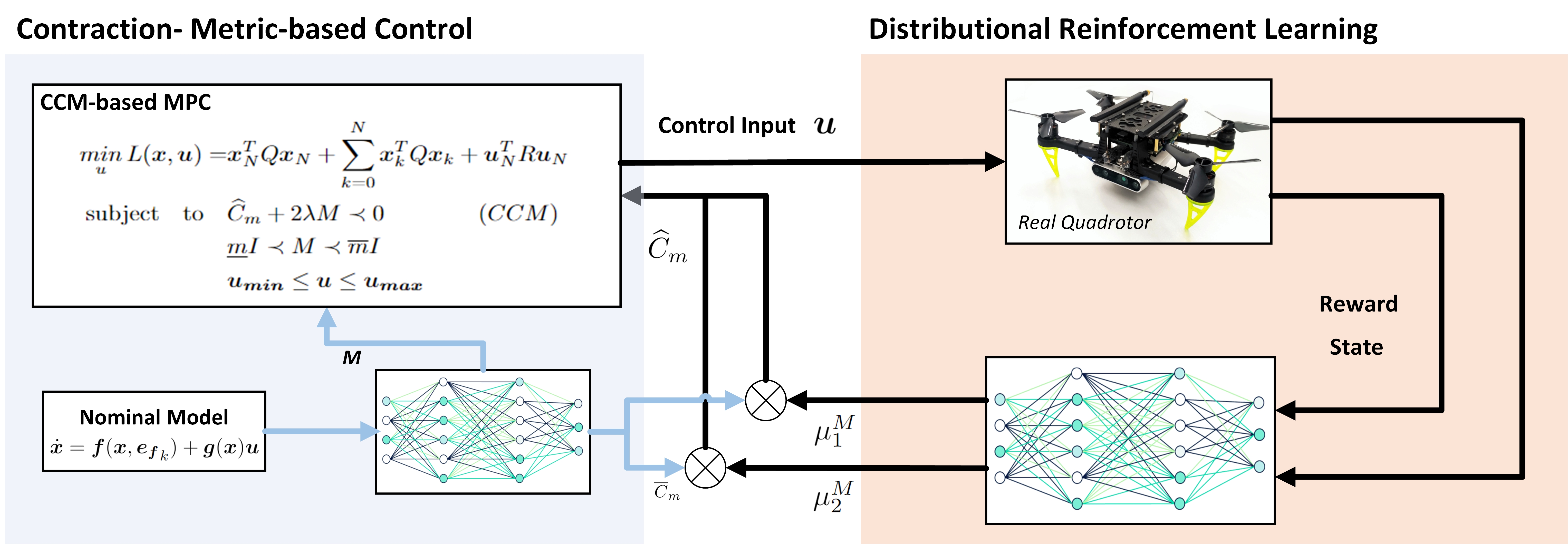
Figure 1: QuaDUE-CCM: a distributional-RL-based estimator and a CCM-based controller

To address these concerns, two areas of research have emerged. The first uses a distributional Reinforcement Learning (RL) [6] method to interact with the complex and changeable uncertainties. The second extends the contraction theory [7] to a control-affine system, called Control Contraction Metric (CCM). This contraction certificate guarantees that the system will exponentially converge to track any feasible reference trajectory [8]. In applications such as quadrotor tracking, we are concerned with the whole tracking process rather than just stabilizing to a fixed point. One common problem with certificate control approaches, like CCM-based control, is that they heavily rely on the accurate knowledge of the system model. Thus, when the model is uncertain, robust or adaptive versions must be considered.

We propose Quantile-approximation-based Distributional Uncertainty Estimatior for Control Contraction Metric (QuaDUE-CCM), as a precise, reliable and systematic quadrotor tracking framwork for use with high variance aerodynamic effects. Our contributions can be summarized: 1) QuaDUE, a distributional-RL-based uncertainty estimator with quantile approximation that can sufficiently estimate variable uncertainties of contraction metrics. In the cases tested, we show that QuaDUE outperforms traditional RL, such as Deep Deterministic Policy Gradient (DDPG) [9], and prior Distributional RL approaches, such as C51 [6]; 2) QuaDUE-CCM, a quadrotor trajectory tracking framework that integrates a distributional-RL-based uncertainty estimator into a CCM-based nonlinear optimal control problem; and 3) Convergence guarantee and acceleration analysis: theoretical understanding and mathematical proofs are provided, i.e., the convergence and acceleration for the interpretability of the distributional RL.

2 Related Work

Quadrotor Uncertainty Modelling: Precise dynamics modeling in quadrotor autonomous navigation is challenging, since a great variety of aerodynamic effects, such as unknown drag coefficients and wind gusts, can be generated by agile flight in high speeds and accelerations. Data-driven approaches, such as Gaussian Processes (GP) [1, 10] and neural networks [11] combined with Model Predictive Control (MPC), have been shown accurate modelling of aerodynamic effects. Due to the nonparametric nature of GP, the GP-based approach hardly scale to the large datasets of complex environments [12]. While neural network-based approaches learn the nonlinear dynamical effects more accurately [13], achieving adaptability and robustness from these learning-based approaches are still ongoing challenges. One important reason is that these training datasets are collected from simulation and/or real-world historical records, from which it is difficult to fully describe the complexity in their environments [14].

Reinforcement Learning for uncertainty: Compared with the existing GP-based and neural-network-based approaches, RL, an adaptive and interactive learning approach, is introduced to model highly dynamic uncertainties in recent work [15]. Distributional RL constructs the entire distributions of the action-value function instead of the traditional expectation, where, to some extent, it addresses the key challenge of traditional RL, i.e., biasing the actions with high variance values in policy optimization [9]. Since some of these values will be overestimated by random chance [16], such actions should be avoided in risk-sensitive or safety-critical applications such as autonomous quadrotor navigation. More importantly, recent work [17] shows that the distributional RL has better interpretability, where we can understand or even accelerate the entire RL training process. This is an encouraging trend, especially for safety-critical applications such as quadrotor autonomous navigation, towards closing the gap between theory and practice in distributional RL.

Control Certificate Techniques: Control certificate techniques guarantee the synthesis of control policies and certificates [18], where the controller can optimize control policies whilst ensuring the satisfaction of the certificate properties. A Control Lyapunov Function (CLF)-based controller [19] ensures that the system state is Lyapunov stable, and a Control Barrier Function (CBF)-based controller [20] ensures that the system state is maintained in defined safety sets given by the barrier function. Contraction is a property of the closed-loop system [7]. [21] reformulates the CCM certificate as a Linear Matrix Inequality problem and solves using Sum-of-Squares (SoS). However, the SoS-based approach cannot extend to general robot systems since an assumption is that the system dynamics need to be polynomial equations or can be approximated as polynomial equations. Then [22, 23] propose a contraction-metric-based control framework, which extends neural networks to certificate learning for contraction metrics. Moreover, based on the framework proposed by Tsukamoto et al., [24, 25, 26, 8] are used to address higher dimensional control problems.

3 Preliminaries and notations

Nominal Quadrotor Dynamic Model and its Control-affine Form: the quadrotor is assumed as a six Degrees of Freedom (DoF) rigid body of mass $m$, i.e., three linear motions and three angular motions [1]. Different from [27, 28], the aerodynamic effect (disturbance) $\bm{e}_{f}$ is integrated into the quadrotor dynamic model as follows [10]:

$$\dot{\bm{P}}_{WB}=\bm{V}_{WB}\qquad\dot{\bm{V}}_{WB}=\bm{g}_{W}+\frac{1}{m}(\bm{q}_{WB}\odot\bm{c}+\bm{e}_{f})$$ (1)

$$\dot{\bm{q}}_{WB}=\frac{1}{2}\Lambda(\bm{\omega}_{B})\bm{q}_{WB}\qquad\dot{\bm{\omega}}_{B}=\bm{J}^{-1}(\bm{\tau}_{B}-\bm{\omega}_{B}\times J\bm{\omega}_{B})$$

where $\bm{P}_{WB}$, $\bm{V}_{WB}$ and $\bm{q}_{WB}$ are the position, linear velocity and orientation expressed in the world frame, and $\bm{\omega}_{B}$ is the angular velocity expressed in the body frame (more detailed definitions please see [10]). Then we reformulate Equation 14 in its control-affine form: $\dot{\bm{x}}=\bm{f}(\bm{x},{\bm{e_{f}}}_{k})+\bm{g}(\bm{x})\bm{u}+\bm{w}$, Where $\bm{f}:\mathbb{R}^{n}\mapsto\mathbb{R}^{n}$ and $\bm{g}:\mathbb{R}^{n}\mapsto\mathbb{R}^{n\times m}$ are assumed by the standard as Lipschitz continuous [29, 8]. $\bm{x}=[\bm{P}_{WB},\bm{V}_{WB},\bm{q}_{WB},\bm{\omega}_{B}]^{T}\in\mathbb{X}$, $\bm{u}=T_{i}\forall i\in(0,3)\in\mathbb{U}$ and $\bm{w}\in\mathbb{W}$ are the state, input and additive uncertainty of the dynamic model, where $\mathbb{X}\subseteq\mathbb{R}^{n}$, $\mathbb{U}\subseteq\mathbb{R}^{n_{u}}$ and $\mathbb{W}\subseteq\mathbb{R}^{n_{w}}$ are compact sets as the state, input and uncertainty space, respectively. Given an input $:\mathbb{R}^{\geq 0}\mapsto\mathbb{U}$ and an initial state $x_{0}\in\mathbb{X}$, our goad is to design a quadrotor tracking controller $\bm{u}$ such that the state trajectory $\bm{x}$ can track any reference state trajectory $\bm{x}_{ref}$ (satisfied the quadrotor dynamic limits) under a bounded uncertainty $\bm{w}:\mathbb{R}^{\geq 0}\mapsto\mathbb{W}$.

Control Contraction Certificates: most existing methods on quadrotor trajectory tracking have so far been demonstrated in stabilization, i.e., a fixed-point-tracking controller [29, 30, 14]. These fixed-point-tracking controllers are relatively efficient in a low-speed and low-variance trajectory. However, to track a high-speed and high-variance trajectory in agile flight, we need a broader specification [31] rather than Lyapunov guarantees that simply stabilize in a fixed point.

Contraction theory [7] gives an analysis on the convergence evolution between the pairs of close trajectories in nonlinear systems, i.e., incremental stability. When extended to a control-affine system, the change rate is defined as $\delta\bm{\dot{x}}=A(\bm{x},\bm{u}){\delta\bm{x}}+B(\bm{x}){\delta\bm{u}}$, where $A(\bm{x},\bm{u}):={\frac{\partial\bm{f}(\bm{x})}{\partial\bm{x}}}+\sum_{i=1}^{m}{u^{i}}{\frac{\partial b_{i}}{\partial\bm{x}}}$,$B(\bm{x})=\bm{g}(\bm{x})$, $b_{i}$ is the $i$-th vector of $B$, and $u^{i}$ is the $i$-th element of $\bm{u}$. Just as a CLF is an extension from the idea of Lyapunov function $V(\bm{x}):\mathbb{X}\mapsto\mathbb{R}$, the contraction theory has been extended to a CCM $M(\bm{x}):\mathbb{X}\mapsto\mathbb{R}^{n\times n}$, i.e., a distance measurement between neighboring trajectories (a contraction metric) that shrinks exponentially, for tracking controller design [32, 33, 34]. As the matrix-valued function $M(\bm{x})$ denotes a symmetric and continuously differentiable metric, ${\delta\bm{x}^{T}}M{\delta\bm{x}}$ defines a Riemannian manifold [35, 7]. If there exists $M\succ 0$ (uniformly positive definite) and exponential convergence of $\delta\bm{x}$ to $0$, the Riemannian infinitesimal length will converge to $0$, then the system is contraction. We have the following theorem:

Theorem 1 (Contraction Metric [7, 31]): In a control-affine system, if there exists: $\dot{M}+{\rm{sym}}(M(A+BK))+2\lambda M\prec 0$, then the inequality $\left\|\bm{x}(t)-\bm{x}_{ref}(t)\right\|\leq Re^{-\lambda t}\left\|\bm{x}(0)-\bm{x}_{ref}(0)\right\|$ with $\forall t\geq 0$, $R\geq 1$ and $\lambda\textgreater 0$ holds, where $A=A(\bm{x},\bm{u})$ and $B=B(\bm{x})$ are defined above, and $\dot{M}={\partial_{f(\bm{x})+g(\bm{x})u}}M=\sum_{i=1}^{n}{\frac{\partial M}{\partial x^{i}}\dot{x}^{i}}$, ${\rm{sym}}(M)=M+M^{T}$, and $\bm{x}_{ref}(t)$ is a sequential reference trajectory. Therefore, we say the system is contraction.

Overview of the Control Framework: the overall framework is shown in Fig. 3. The aim of this work is to design a quadrotor controller, which combines wind estimation - i.e., VID-Fusion [36], for tracking the reference trajectory $\bm{x}_{ref}(t)$ of the nominal model (Equation 14) under highly variable aerodynamic disturbances. We propose a CCM-based MPC, where the parameter $\theta$ corresponds to weights of a neural network that estimates the uncertainty $\Delta_{1}$ and $\Delta_{2}$ in the CCM dynamics. Combining with the neural network, a Distributional-RL-based Estimator, i.e., QuaDUE, is used to learn the uncertainties adaptively whilst satisfying the constraints of the contraction metric.

4 Distributional Reinforcement Learning for CCM

Quantile-approximation-based Distributional-reinforced Uncertainty Estimator: in policy evaluation setting, given a 5-tuple Markov Decision Process [37]: $MDP:=\left\langle S,A,P,R,\gamma\right\rangle$ (where $S$, $A$, $P$, $R$ and $\gamma\in[0,1]$ are the state spaces, action spaces, transition probability, immediate reward function and discount rate), a distributional Bellman equation defines the state-action distribution $Z$ and the Bellman operator $\mathcal{T}^{\pi}$ as [6, 38]: $\mathcal{T}^{\pi}Z(\bm{s},\bm{a})\overset{D}{:=}R(\bm{s},\bm{a})+\gamma Z(\bm{s^{\prime}},\bm{a^{\prime}})$, where $\bm{s}\in S$ and $\bm{a}\in A$ are the state and action vector. $\pi$ is a deterministic policy under the policy evaluation. In policy control setting, based on the quantile approximation [38], the distributional Bellman optimality operator $\mathcal{T}$ is defined as: $\mathcal{T}Z(\bm{s},\bm{a})\overset{D}{:=}R(\bm{s},\bm{a})+\gamma Z(\bm{s^{\prime}},{\rm{arg}}\underset{a^{\prime}}{max}\underset{\bm{p},R}{\mathbb{E}}[Z(\bm{s^{\prime}},\bm{a^{\prime}})])$ where $Z_{\theta}(\bm{s},\bm{a}):=\frac{1}{N}\sum\limits_{i=1}^{N}\delta_{q_{i}(\bm{s},\bm{a})}\in Z_{Q}$ is a quantile distribution mapping one state-action pair $(s,a)$ to a uniform probability distribution supported on $q_{i}$. $Z_{Q}$ is the space of quantile distribution within $N$ supporting quantiles. $\delta_{z}$ denotes a Dirac with $z\in\mathbb{R}$. Then the maximal form of the Wasserstein metric is proved to be a contraction in [6] as:

$$\overset{-}{d}_{\infty}(\Pi_{W_{1}}\mathcal{T}^{\pi}Z_{1},\Pi_{W_{1}}\mathcal{T}^{\pi}Z_{2})\leq\overset{-}{d}_{\infty}(Z_{1},Z_{2})$$ (2)

where $W_{p}$, $p\in[1,\infty]$ denotes the $p$-Wasserstein distance. $\overset{-}{d}_{p}:={\rm{sup}}W_{p}(Z_{1},Z_{2})$ denotes the maximal form of the $p$-Wasserstein metrics. $\Pi_{W_{1}}$ is a quantile approximation under the minimal 1-Wasserstein distance $W_{1}$.

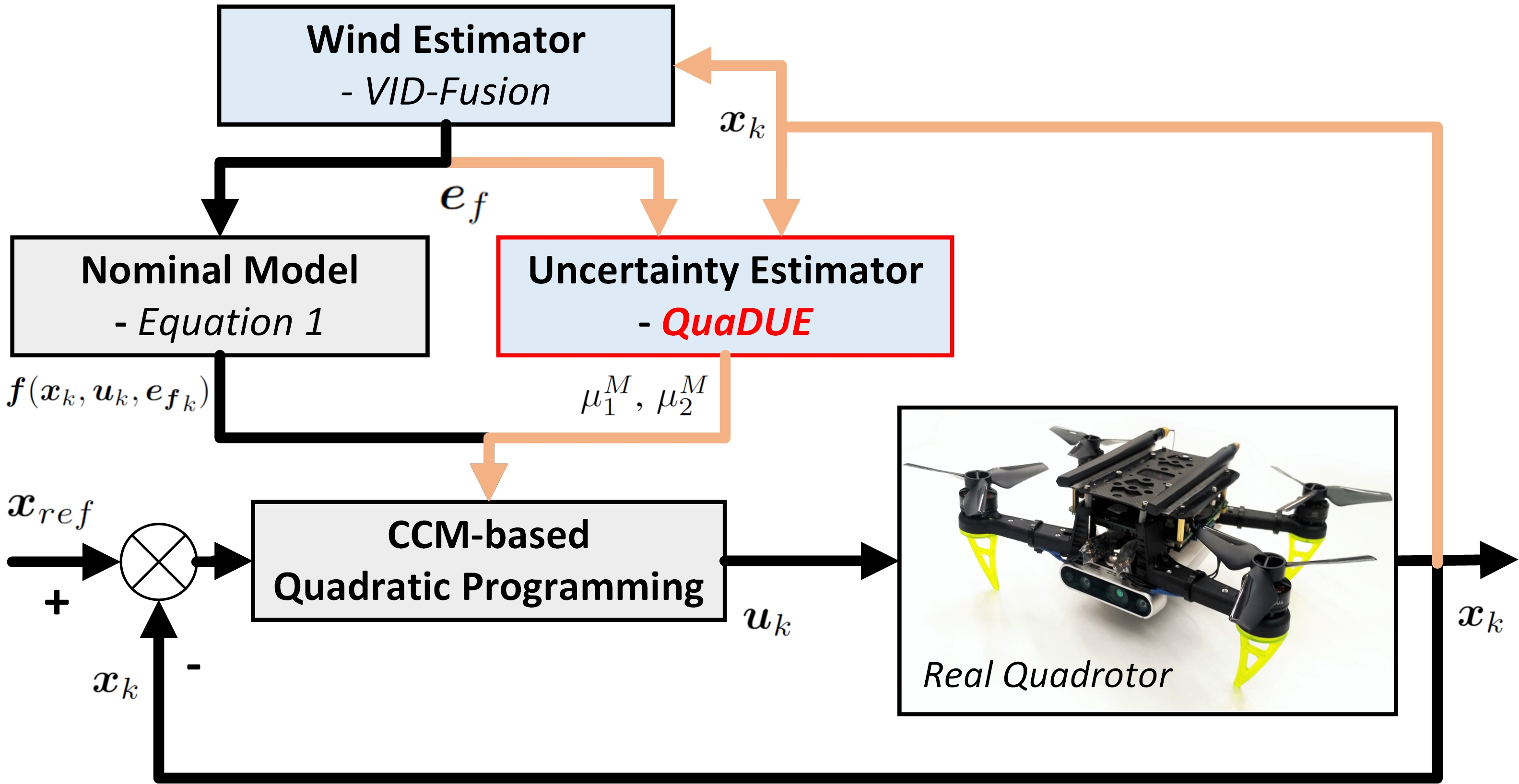
Figure 2: The position of QuaDUE-CCM in the Quadrotor system:

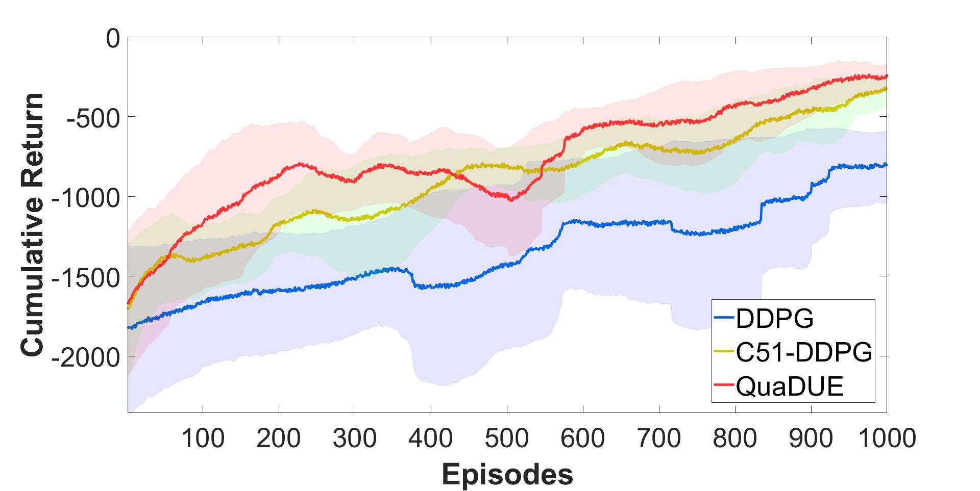
Figure 3: Learning curves of RL algorithms. The simulated speed is set as $0.4$.

Distributional-RL-based Estimator for CCM Uncertainty: denoting $\dot{M}+{\rm{sym}}(M(A+BK))$ in Theorem 1 by $\overline{C}_{m}(\bm{x},\bm{x}_{ref},\bm{u}_{ref},\theta_{nominal-metric})$, where $\theta_{nominal-metric}$ is the parameter of the neural network in the contraction metric learning [8] for the nominal function Equation 14 with $\bm{e}_{f}=0$, then the truth $C_{m}$ under uncertainty becomes: ${C}_{m}=\sum_{i=1}^{n}{\frac{\partial M}{\partial x^{i}}\dot{x}^{i}}+{\rm{sym}}(M(A+BK))+\Delta_{1}^{M}(x)+\Delta_{2}^{M}(x)u=\overline{C}_{m}+\Delta_{1}^{M}(x)+\Delta_{2}^{M}(x)u$ .

We employ an agent of QuaDUE to estimate the uncertain terms in $\widehat{C}_{m}$: $\Delta_{1}^{M}(x)$ and $\Delta_{2}^{M}(x)$. Therefore, an estimation $\widehat{C}_{m}$ is constructed by:$\widehat{C}_{m}=\overline{C}_{m}+\mu_{\theta_{rl},1}^{M}(x)+\mu_{\theta_{rl},2}^{M}(x)u$, where $[\mu_{\theta_{rl},1}^{M}(x),\mu_{\theta_{rl},2}^{M}(x)]$ - i.e., a symmetric matrix - is the output (action) of QuaDUE. $\theta_{rl}$ is again the neural network parameters. Then our goal of the Distributional-RL-based Estimator - i.e., QuaDUE - is clear: learn a policy $\mu_{1}^{M}$, $\mu_{2}^{M}$ such that the estimation $\widehat{C}_{m}$ as close as to the true value ${C}_{m}$. Notice here that we use the same neural network $\theta_{rl}$ for $\mu_{\theta_{rl},1}^{M}(x)$ and $\mu_{\theta_{rl},2}^{M}(x)$. In Section 5 below, we will demonstrate our reasoning and give proof.

A framework of QuaDUE is illustrated in Fig.1. The QuaDUE learns a policy which combines with the CCM uncertainties $\Delta_{1}^{M}(x)$, $\Delta_{2}^{M}(x)$ and other dynamic constraints. Then we design the reward function as $R_{t+1}(s,a,\theta)=R_{contraction}(s,a,\theta)+R_{track}(s,a)$, where $\theta\in\Theta$ represents the neural network parameters. Thus, the reward function is defined in detail as:

$$R_{contraction}(s,a,\theta)= -\omega_{c,1}[\underline{m}I-M]_{ND}{(s)}-\omega_{c,2}[M-\overline{m}I]_{ND}{(s)}$$ (3)

$$-\omega_{c,3}[\widehat{C}_{m}+2\lambda M]_{ND}{(s,a,\theta)}$$

$$R_{track}(s,a)= -(\bm{x}_{t}{(s,a)}-\bm{x}_{ref,t})^{\rm{T}}H_{1}(\bm{x}_{t}{(s,a)}-\bm{x}_{ref,t})-\bm{u}_{t}^{\rm{T}}{(s,a)}H_{2}\bm{u}_{t}{(s,a)}$$

where $\underline{m}$, $\overline{m}$ are hyper-parameters, $H_{1}$ and $H_{2}$ are positive definite matrices, and $\bm{[}A\bm{]}_{ND}$ is for penalizing positive definiteness where $\bm{[}A\bm{]}_{ND}=0$ iff. $A\prec 0$, and $\bm{[}A\bm{]}_{ND}\geq 0$ iff. $A\succeq 0$.

These QuaDUE outputs, i.e., $\mu_{\theta_{rl},1}^{M}(x)$ and $\mu_{\theta_{rl},2}^{M}(x)$, are then fed into the CCM constraints derived from the nominal model. Specifically, the estimated $\widehat{C}_{m}$ is used as the best guess of ${C}_{m}$ for MPC to satisfy the true constraints. The MPC formulation combining with CCM constraints are shown in Fig. 1, where the learned uncertainties are used to construct the contraction constraints of the MPC. Then the MPC is specified to a quadratic optimization formulation and implemented using CasADi [39] and ACADOS [40].

5 Properties of QuaDUE: Convergence and Acceleration analysis

In this section, the properties of the proposed Distributional-RL-based Estimator - i.e., QuaDUE - are analyzed, including convergence guarantees and training acceleration analysis. In particular, we empirically verify a more stable and accelerated convergence process than traditional RL algorithms (shown in Section 6), and demonstrate a theoretical understanding of the proposed QuaDUE.

Convergence Analysis of QuaDUE: Equation 5 shows that the Bellman operator $\mathcal{T}^{\pi}$ is a $p$-contraction under the $p$-Wasserstein metric $\overset{-}{d}_{p}$ [6]. The Wasserstein distance $W_{p}$ between a distribution $Z$ and its Bellman update $\mathcal{T}^{\pi}Z$ can be minimized iteratively in Temporal Difference learning. Therefore, we present the convergence analysis of QuaDUE for Policy Evaluation and Policy Improvement, respectively.

Proposition 2 (Policy Evaluation [38, 14]): Given a deterministic policy $\pi$, a quantile approximator $\Pi_{W_{1}}$ and $Z_{k+1}(\bm{s},\bm{a})=\Pi_{W_{1}}\mathcal{T}^{\pi}Z_{k}(\bm{s},\bm{a})$, the sequence $Z_{k}(\bm{s},\bm{a})$ converges to a unique fixed point $\overset{\sim}{Z_{\pi}}$ under the maximal form of $\infty$-Wasserstein metric $\overset{-}{d}_{\infty}$.

Proposition 3 (Policy Improvement [14]): Denoting an old policy by $\bm{\pi}_{\bm{old}}$ and a new policy by $\bm{\pi}_{\bm{new}}$, there exists $\mathbb{E}[Z(s,a)]^{\bm{\pi}_{\bm{new}}}(s,a)\geq\mathbb{E}[Z(s,a)]^{\bm{\pi}_{\bm{old}}}(s,a)$, $\forall s\in\mathcal{S}$ and $\forall a\in\mathcal{A}$.

Based on Proposition 2 and Proposition 3, we are ready to present Theorem 4 to demonstrate the convergence of QuaDUE.

Theorem 4 (Convergence): Denoting the policy of the $i$-th policy improvement by $\bm{\pi}^{\bm{i}}$, there exists $\bm{\pi}^{\bm{i}}\rightarrow\bm{\pi}^{*}$, $i\rightarrow\infty$, and $\mathbb{E}[Z_{k}(s,a)]^{\bm{\pi}^{*}}(s,a)\geq\mathbb{E}[Z_{k}(s,a)]^{\bm{\pi}^{\bm{i}}}(s,a)$, $\forall s\in\mathcal{S}$ and $\forall a\in\mathcal{A}$.

Proof: Proposition 3 shows that $\mathbb{E}[Z(s,a)]^{\bm{\pi}^{\bm{i}}}\geq\mathbb{E}[Z(s,a)]^{\bm{\pi}^{\bm{i-1}}}$, thus $\mathbb{E}[Z(s,a)]^{\bm{\pi}^{\bm{i}}}$ is monotonically increasing. According to Equation 5 and Equation 10, the first moment of $Z$, i.e., $\mathbb{E}[Z(s,a)]^{\bm{\pi}^{\bm{i}}}$, is upper bounded. Therefore, the sequential $\mathbb{E}[Z(s,a)]^{\bm{\pi}^{\bm{i}}}$ converges to an upper limit $\mathbb{E}[Z(s,a)]^{\bm{\pi}^{*}}$ satisfying $\mathbb{E}[Z_{k}(s,a)]^{\bm{\pi}^{*}}(s,a)\geq\mathbb{E}[Z_{k}]^{\bm{\pi}^{\bm{i}}}$. $\blacksquare$

Training Acceleration of QuaDUE: training acceleration is investigated for our QuaDUE in order to guarantee a more stable and predictable RL training process. For implementation execution, we use Kullback-Leibler (KL) divergence [41] instead of Wasserstein Metric. KL divergence is proven and implemented ’usable’ in [6]. Thus we use KL divergence to analyze the acceleration in RL training process, which is closer to the real implementation.

Similar to [14], we denote $J_{\theta}(s,a)=D_{KL}(p^{s,a},q^{s,a}_{\theta})$ as the histogram distributional loss, where $p^{s,a}(x)$ and $q^{s,a}_{\theta}$ are the true and approximated density function of $Z(s,a)$. We denote $E_{J}(\theta)=\mathbb{E}_{(s,a)\sim{\rho_{\pi}}}[J_{\theta}(s,a)]$ is the expectation of $J_{\theta}$, where $\rho_{\pi}$ is the generated distribution under the deterministic policy $\pi$. Since the unbiased gradient estimation of KL divergence, there exits $\mathbb{E}_{(s,a)\sim{\rho_{\pi}}}[\left\|\nabla J_{\theta}({p_{\mu}}^{s,a},q^{s,a}_{\theta})-\nabla E_{J}(\theta)\right\|^{2}]=\kappa\sigma^{2}$, where we represent the approximation error between ${p_{\mu}}^{s,a}$ and $q^{s,a}_{\theta}$. A good degree of the approximation leads to a small $\kappa$, which then effects the training acceleration of the distribution RL [17], as shown in Theorem 5.

Next we define a stationary-point for the derivative of $E_{J}(\theta)$ [17]: if there exits $\left\|\nabla E_{J}(\theta_{T})\right\|\leq\tau$ ($\tau\in(0,1)$), the updated parameters $\theta_{T}$ after $T$ steps is a first-order $\tau$-stationary point. Then we immediately present Theorem 5 for the training acceleration.

Theorem 5 (Training Acceleration): In the training process of the distribution RL (i.e., QuaDUE):

1) Let sampling steps $T=4k{l^{2}}{E_{J}}(\theta_{0})/\tau^{2}$, if there exists $\kappa\leq 0.25{\tau^{2}}/\sigma^{2}$, the $J_{\theta}$ optimized by stochastic gradient descend converges to a $\tau$-stationary point.

2) Let sampling steps $T=k{l^{2}}{E_{J}}(\theta_{0})/(\kappa\tau^{2})$, if there exists $\kappa>0.25{\tau^{2}}/\sigma^{2}$, the $J_{\theta}$ optimized by stochastic gradient descend will not converge to a $\tau$-stationary point.

Proof: As $J_{\theta}(p^{s,a},a^{s,a}_{\theta})$ is $kl^{2}$-smooth, we have: $E_{J}(\theta_{t+1})-E_{J}(\theta_{t})\leq\langle\nabla E_{J}(\theta_{t}),\theta_{t+1}-\theta_{t}\rangle+(kl^{2}/2)\left\|\theta_{t+1}-\theta_{t}\right\|^{2}=-\lambda\langle\nabla E_{J}(\theta_{t}),\nabla J_{\theta}(p^{s,a},a^{s,a}_{\theta})\rangle+({kl^{2}}\lambda^{2}/2)\left\|\nabla J_{\theta}(p^{s,a},a^{s,a}_{\theta})\right\|^{2}\\ \leq-(\lambda/2)\left\|\nabla E_{J}(\theta_{t})\right\|^{2}+(\lambda/2)\left\|\nabla E_{J}(\theta_{t})-J_{\theta}(p^{s,a},a^{s,a}_{\theta})\right\|^{2}$, where $\lambda=1/kl^{2}$.

Next we take the expected value and consider $T$ steps: $\mathbb{E}[E_{J}(\theta_{T})-E_{J}(\theta_{0})]\leq\mathbb{E}[\sum_{t=0}^{T-1}-(\lambda/2)\left\|\nabla E_{J}(\theta_{t})\right\|^{2}]+\mathbb{E}[\sum_{t=0}^{T-1}(\lambda/2)\left\|\nabla E_{J}(\theta_{t})-J_{\theta}(p^{s,a},a^{s,a}_{\theta})\right\|^{2}]\leq-(\lambda/2)\sum_{t=0}^{T-1}\mathbb{E}[\left\|\nabla E_{J}(\theta_{t})\right\|^{2}]+(\lambda/2)[(1-1/(1+\kappa))\sigma^{2}+(\kappa/(1+\kappa))\sigma^{2}]$. If we have a first-order stationary point at $T$ step, then:

$$(1/T)\sum_{t=0}^{T-1}\mathbb{E}[\left\|\nabla E_{J}(\theta_{t})\right\|^{2}]\leq 2kl^{2}E_{J}(\theta_{0})/T+2\kappa\sigma^{2}$$ (4)

If we have $T=4k{l^{2}}{E_{J}}(\theta_{0})/\tau^{2}$ and $\kappa\leq 0.25{\tau^{2}}/\sigma^{2}$, then $J_{\theta}$ converges to a $\tau$-stationary point with $(1/T)\sum_{t=0}^{T-1}\mathbb{E}[\left\|\nabla E_{J}(\theta_{t})\right\|^{2}]\leq\tau^{2}$. Thus, (1) is proved. If we have $T=k{l^{2}}{E_{J}}(\theta_{0})/(\kappa\tau^{2})$ and $\kappa>0.25{\tau^{2}}/\sigma^{2}$, then $(1/T)\sum_{t=0}^{T-1}\mathbb{E}[\left\|\nabla E_{J}(\theta_{t})\right\|^{2}]\leq 4\kappa\tau^{2}$, where the stationary point is depended on $\kappa$, i.e., the degree of the approximation. Therefore, (2) is proved. $\blacksquare$

Theorem 5 demonstrates two cases of training acceleration in our QuaDUE. In (1) of Theorem 5, the convergence of QuaDUE is accelerated where there is a low approximation error $\kappa$ between $p^{s,a}(x)$ and $q^{s,a}_{\theta}$. In (2) of Theorem 5, a relatively larger $\kappa>0.25{\tau^{2}}/\sigma^{2}$ will give no guarantee for acceleration convergence. But if $(1/T)\sum_{t=0}^{T-1}\mathbb{E}[\left\|\nabla E_{J}(\theta_{t})\right\|^{2}]\leq 4\kappa\tau^{2}$ is satisfied, the distributional RL still converges to the stationary optimization point. This understanding from theoretical analysis is consistent with our empirical experiment results in Section 6: when we add small external forces (disturbances) in the specific scenarios Fig. 5, the performance of the two distributional RL - i.e., ‘QuaDUE-CCM’ and ‘QuaDRED-MPC’ - is less than ‘DDPG-CCM’. The cases in [38] also verify this observation from simple Atari games.

6 Evaluation of Performance

To evaluate the performance of the proposed QuaDUE-CCM, we compare against the convergence

Table 1: Parameters of QuaDUE-CCM

Parameters Definition Values $l_{\theta_{a}}$ Learning rate of actor 0.0015 $l_{\theta_{c}}$ Learning rate of critic 0.0015 $\theta_{a}$ Actor neural network: fully connected with two hidden layers (128 neurons per hidden layer) - $\theta_{c}$ Critic neural network: fully connected with two hidden layers (128 neurons per hidden layer) - $D$ Replay memory capacity $10^{4}$ $B$ Batch size 256 $\gamma$ Discount rate 0.9995 - Training episodes 1000 $T_{s}$ MPC Sampling period 50ms $N$ Time steps 20

performance of DDPG [9], C51-DDPG [6] in training process, the tracking performance of GP-MPC [1, 10], DDPG-CCM and QuaDRED-MPC [14] under highly variable aerodynamic disturbances (uncertainties). The parameters of our QuaDUE-CCM are summarized in Table 3 according to the benchmark works (see [1, 14, 42]).

Comparative Performance of QuaDUE Training: we have two main training process: firstly, we employ a certified learning controller proposed in [8, 31] to learn a Contraction Metric for the nominal model (Equation 14) as shown in Fig. 1. Then we operate a training process by generating external forces in RotorS [43], where the programmable external forces are in the horizontal plane with range [-3,3] ($m/s^{2}$). The training process has 1000 iterations where the quadrotor state is recorded at 16 $Hz$. The convergence curves of the training are illustrated in Fig. 3, where we show the comparative training performance of DDPG, C51-DDPG and our QuaDUE. Our performance illustrates that the two distributional RL approaches, C51-DDPG and QuaDUE, outperform the traditional DDPG RL approach, whilst our proposed QuaDUE achieves the largest cumulative return. More importantly, our QuaDUE maintains the highest convergence speed, which again verifies the theoretical guarantees demonstrated in Section 5.

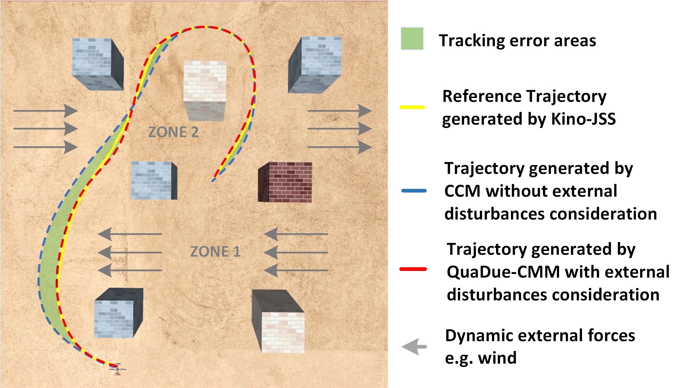
Figure 4: The simulation scenario in RotorS: both reference trajectories with/without external forces are generated by Kino-JSS [10].

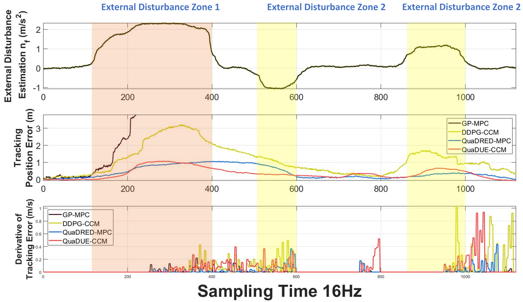
Figure 5: Specific scenarios results: Wind estimation $\bm{n}_{f}$ (expressed in body frame), position error $(m)$ and derivatives of tracking error.

Comparative Performance of QuaDUE-CCM in Variable Aerodynamic Disturbance: we evaluate our proposed QuaDUE-CCM with variable aerodynamic forces generated in ZONE 1 and ZONE 2 of the specific scenario, as described in Fig. 5. We compare the tracking position errors and derivatives of tracking error with different and opposite heading aerodynamic forces with [0.0, 1.5, 0.0] $m/s^{2}$ and [0.0, -1.0, 0.0] $m/s^{2}$ in ZONE 1 and ZONE 2, respectively. As shown in Fig. 5, the three benchmarks are: 1) GP-MPC, a state-of-the-art trajectory tracking method; 2) DDPG-CCM, an adaptive approach extending from RL-CBF-CLF-QP [29] to solve the CCM uncertainties along with a nonlinear MPC; 3) QuaDRED-MPC, a novel learning-based MPC for uncertainties combining with a distributional RL agent and a nonlinear MPC.

In Fig. 5, the two distributional-RL-estimator-based frameworks (i.e., QuaDRED-MPC and QuaDUE-CCM) react to the sudden aerodynamic effects more sufficiently than the traditional RL-based estimator (i.e., DDPG).

Table 2: Comparison of Trajectory Tracking under Programmatic External forces

Ex. Forces ($m/s^{2}$) Method Succ. Rate Time (s) Err. (m) Contra. Rate ($\lambda/C$) Z1: [0, 0.5, 0.0] Z2: [0, -0.5, 0.0] GP-MPC 100% 23.54 3.44 0.097~0.63/6.49 DDPG + CCM 97.6% 24.11 3.82 0.285~1.01/3.54 QuaDRED-MPC 95.3% 25.54 4.30 0.100~0.64/6.41 QuaDUE-CCM 95.1% 25.84 4.78 0.302~1.07/3.54 Z1: [0, 2.5, 0.0] Z2: [0, -2.5, 0.0] GP-MPC 69.8% 38.62 24.27 0.093~0.61/6.53 DDPG + CCM 79.8% 33.10 18.62 0.240~0.92/3.83 QuaDRED-MPC 89.1% 29.57 14.93 0.089~0.58/6.49 QuaDUE-CCM 87.2% 30.19 15.49 0.278~1.01/3.63 Z1: [-3.0, 3.5, 0.0] Z2: [-2.0, -2.0, 0.0] GP-MPC 0% - - - DDPG + CCM 48.5% 43.64 27.24 0.257~0.81/3.85 QuaDRED-MPC 83.3% 36.40 17.66 0.079~0.53/6.69 QuaDUE-CCM 84.1% 36.45 17.13 0.265~0.95/3.59

Among the two distributional-based methods, the QuaDRED-MPC’s tracking performance is slightly better (accumulated error $6.73\%$ less) than our proposed QuaDUE-CCM. This is mainly because the QuaDRED-MPC assesses the environment uncertainties and then directly feeds the uncertainty estimation into the nominal model while the QuaDUE-CCM is an indirect method required to satisfy the contraction metrics, which makes the tracking actions more conservative. However, based on the contraction theory, our proposed QuaDUE-CCM has $20.7\%$ bigger derivative of tracking error than QuaDRED-MPC and the contraction rate is $Ce^{-\lambda t}$ with $C=3.59$ and $\lambda=1.046$. This again means that, under variable uncertainties, our QuaDUE-CCM converges to a reference trajectory in a higher contraction rate (exponential contraction) both with theoretical (contraction theory) and empirical guarantees.

Then larger and more complex external forces, i.e., [-2.5, 2.5, 0.0] and [-3.0, 3.0, 0.0] ($m/s^{2}$), are generated in ZONE 1 and ZONE 2, respectively, as shown in Fig. 5. In Table 2, we compare the success rate, operation time, accumulated tracking error and contraction rate with the corresponding variable external forces in ZONE 1 and ZONE 2. Our results show that RL-based methods are not always better, especially with relatively small external forces. For example, the success rate of RL-based methods (i.e., ‘DDPG + CCM’, ‘QuaDRED-MPC’ and ‘QuaDUE-CCM’) is lower than ’GP-MPC’. We also find that the two distributional-RL-based methods have close tracking errors, where in some cases ‘QuaDRED-MPC’ is sightly better than ‘QuaDUE-CCM’. However, compared to ‘QuaDRED-MPC’, our ‘QuaDUE-CCM’ achieves 302% , 312% and 335% improvements in contraction rate.

7 Conclusion

In this paper, we propose a precise and reliable trajectory tracking framework, QuaDUE-CCM, for quadrotors in dynamic and unknown environments with highly variable aerodynamic effects. QuaDUE-CCM combines a distributional-RL-based uncertainty estimator and CCMs to address large and variable uncertainties on quadrotor tracking. A Quantile-approximation-based Distributional-reinforced Uncertainty Estimator, QuaDUE, is proposed to learn the uncertainties of contraction metrics adaptively, where the convergence and acceleration in the RL training process are analyzed from theoretical perspectives. Based on the contraction theory, CCMs are used to guarantee exponential convergence to any feasible reference trajectory, which significantly improve the reliability of our tracking systems. We empirically demonstrate that our proposed approach can track agile trajectories with at least 36.2% improvement under large aerodynamic effects, where experimental data can favourably verify our theoretical results.

8 Limitation

As mentioned in Sections 5 & 6, in comparison with GP-MPC, our QuaDUE-CCM performs weakly under small disturbances. The potential reasons, as discussed at the end of Sections 5 & 6, are its theoretical attributions and highly variable uncertainties modelling. Our ongoing work concerns incorporating direct uncertainty estimation, i.e., adding uncertainties into controller directly, and certificate-based uncertainty estimation to improve the performance under relatively small uncertainties. Another limitation is the computational complexity, where we use 16 $Hz$ for the CCM uncertainty estimation. To improve this, QuaDUE-CCM may be deployed on dedicated chips, developed via FPGA implementation. We will evaluate the performance in real-world flight tests, in which our system will face a greater variety of aerodynamic disturbances.

Appendix

In this supplementary, Section A shows the detailed definition of Theorem 1 (Contraction Metric), and proof of Proposition 2 (Policy Evaluation), Proposition 3 (Policy Improvement), Theorem 4 (Convergence) and Theorem 5 (Training Acceleration). Section B shows the detailed nominal dynamic model of quadrotor, and its parameters description. Section C shows the algorithm details of QuaDUE, combining with DDPG algorithm. Section D shows the algorithm details of the reference trajectory generation, i.e., Kino-JSS. Section E shows the implementation details of QuaDUE-CCM.

Appendix A Detailed definition of Contraction; and proof of Proposition 2, Proposition 3, Theorem 4 and Theorem 5

Contraction is described as follows. We firstly consider general time-variant autonomous systems $\dot{x}=f_{c}(x,t)$. Then we have $\delta\dot{x}={\frac{\partial f_{c}}{\partial x}}(x,t)\delta x$, where $\delta x$ is a virtual displacement. Next two neighboring trajectories are considered in the field $\dot{x}=f_{c}(x,t)$. The square distance between these two trajectories is defined as ${{\delta x}^{T}}{\delta x}$, where the rate of change is given by $\frac{\mathrm{d}}{\mathrm{d}t}({{\delta x}^{T}}{\delta x})=2{{\delta x}^{T}}{\delta\dot{x}}=2{{\delta x}^{T}}\frac{\partial f_{c}}{\partial x}{\delta x}$. Let $\lambda_{m}(x,t)<0$ be the largest eigenvalue of the symmetrical part of the Jacobian $\frac{\partial f_{c}}{\partial x}$ such that there exists $\frac{\mathrm{d}}{\mathrm{d}t}({{\delta x}^{T}}{\delta x})\leq 2\lambda_{m}{{\delta x}^{T}}{\delta x}$. Therefore we have $\left\|{\delta x}\right\|\leq e^{\int_{0}^{t}\lambda_{m}(x,t)\mathrm{d}t}\left\|{\delta x_{o}}\right\|$. Such a system can be called contraction. Therefore, we have the following Theorem 1.

Theorem 1 (Contraction Metric): In a control-affine system, if there exists: $\dot{M}+{\rm{sym}}(M(A+BK))+2\lambda M\prec 0$, then the inequality $\left\|\bm{x}(t)-\bm{x}_{ref}(t)\right\|\leq Re^{-\lambda t}\left\|\bm{x}(0)-\bm{x}_{ref}(0)\right\|$ with $\forall t\geq 0$, $R\geq 1$ and $\lambda\textgreater 0$ holds, where $A=A(\bm{x},\bm{u})$ and $B=B(\bm{x})$ are defined above, and $\dot{M}={\partial_{f(\bm{x})+g(\bm{x})u}}M=\sum_{i=1}^{n}{\frac{\partial M}{\partial x^{i}}\dot{x}^{i}}$, ${\rm{sym}}(M)=M+M^{T}$, and $\bm{x}_{ref}(t)$ is a sequential reference trajectory. Therefore, we say the system is contraction.

Proof can be found in [7, 31].

Proposition 2 (Policy Evaluation): Given a deterministic policy $\pi$, a quantile approximator $\Pi_{W_{1}}$ and $Z_{k+1}(\bm{s},\bm{a})=\Pi_{W_{1}}\mathcal{T}^{\pi}Z_{k}(\bm{s},\bm{a})$, the sequence $Z_{k}(\bm{s},\bm{a})$ converges to a unique fixed point $\overset{\sim}{Z_{\pi}}$ under the maximal form of $\infty$-Wasserstein metric $\overset{-}{d}_{\infty}$.

Proof: The combined operator $\Pi_{W_{1}}\mathcal{T}^{\pi}$ is an $\infty$-contraction [38] as there exists:

$$\overset{-}{d}_{\infty}(\Pi_{W_{1}}\mathcal{T}^{\pi}Z_{1},\Pi_{W_{1}}\mathcal{T}^{\pi}Z_{2})\leq\overset{-}{d}_{\infty}(Z_{1},Z_{2})$$ (5)

Then based on the Banach’s fixed point theorem, we have a unique fixed point $\overset{\sim}{Z_{\pi}}$ of $\mathcal{T}^{\pi}$. Since all moments of $Z$ are bounded in $Z_{\theta}(\bm{s},\bm{a}):=\frac{1}{N}\sum\limits_{i=1}^{N}\delta_{q_{i}(\bm{s},\bm{a})}$, obviously, the sequence $Z_{k}(\bm{s},\bm{a})$ converges to $\overset{\sim}{Z_{\pi}}$ in $\overset{-}{d}_{\infty}$ for $p\in[1,\infty]$. $\blacksquare$

Proposition 3 (Policy Improvement: Denoting an old policy by $\bm{\pi}_{\bm{old}}$ and a new policy by $\bm{\pi}_{\bm{new}}$, there exists $\mathbb{E}[Z(s,a)]^{\bm{\pi}_{\bm{new}}}(s,a)\geq\mathbb{E}[Z(s,a)]^{\bm{\pi}_{\bm{old}}}(s,a)$, $\forall s\in\mathcal{S}$ and $\forall a\in\mathcal{A}$.

Proof: We firstly denote the expectation of $Z(s,a)$ by $Q(s,a)$. Then based on:

$$\mathcal{T}Z(\bm{s},\bm{a})\overset{D}{:=}R(\bm{s},\bm{a}) +\gamma Z(\bm{s^{\prime}},{\rm{arg}}\underset{a^{\prime}}{max}\underset{\bm{p},R}{\mathbb{E}}[Z(\bm{s^{\prime}},\bm{a^{\prime}})])$$ (6)

$$Z_{\theta}(\bm{s},\bm{a}) :=\frac{1}{N}\sum\limits_{i=1}^{N}\delta_{q_{i}(\bm{s},\bm{a})}$$

there exists:

$$V^{\pi}(s_{t}) =\mathbb{E}_{\pi}{Q^{\pi}(s_{t},\pi(s_{t}))}\leq\underset{a\in\mathcal{A}}{\rm{max}}\mathbb{E}_{\pi}{Q^{\pi}(s_{t},a)}=\mathbb{E}_{\pi^{\prime}}{Q^{\pi}(s_{t},{\pi^{\prime}}(s_{t}))}$$ (7)

where $\mathbb{E}_{\pi}[\cdot]=\sum_{a\in A}\bm{\pi}(a|s)[\cdot]$, and $V^{\pi}(s)=\mathbb{E}_{\pi}\mathbb{E}[Z_{k}(s,a)]$ is the value function. According to Equation 6 and Equation 7, it yields:

$$Q^{\bm{\pi}_{\bm{old}}} =Q^{\bm{\pi}_{\bm{old}}}(s_{t},\bm{\pi}_{\bm{new}}(s_{t}))=r_{t+1}+\gamma\mathbb{E}_{s_{t+1}}\mathbb{E}_{\bm{\pi}_{\bm{old}}}Q^{\bm{\pi}_{\bm{old}}}(s_{t+1},{\bm{\pi}_{\bm{old}}}(s_{t+1}))$$ (8)

$$\leq r_{t+1}+\gamma\mathbb{E}_{s_{t+1}}\mathbb{E}_{\bm{\pi}_{\bm{new}}}{Q^{\bm{\pi}_{\bm{old}}}(s_{t+1},{\bm{\pi}_{\bm{new}}}(s_{t+1}))}$$

$$\leq r_{t+1}+\mathbb{E}_{s_{t+1}}\mathbb{E}_{\bm{\pi}_{\bm{new}}}[\gamma r_{t+2}+{\gamma^{2}}\mathbb{E}_{s_{t+2}}{Q^{\bm{\pi}_{\bm{old}}}(s_{t+2},{\bm{\pi}_{\bm{new}}}(s_{t+2}))}|]$$

$$\leq r_{t+1}+\mathbb{E}_{s_{t+1}}\mathbb{E}_{\bm{\pi}_{\bm{new}}}[\gamma r_{t+2}+{\gamma^{2}}r_{t+3}+...]=r_{t+1}+\mathbb{E}_{s_{t+1}}V^{\bm{\pi}_{\bm{new}}}(s_{t+1})$$

$$=Q^{\bm{\pi}_{\bm{new}}}$$

Thus there exists $\mathbb{E}[Z(s,a)]^{\bm{\pi}_{\bm{new}}}(s,a)\geq\mathbb{E}[Z(s,a)]^{\bm{\pi}_{\bm{old}}}(s,a)$. $\blacksquare$

Theorem 4 (Convergence): Denoting the policy of the $i$-th policy improvement by $\bm{\pi}^{\bm{i}}$, there exists $\bm{\pi}^{\bm{i}}\rightarrow\bm{\pi}^{*}$, $i\rightarrow\infty$, and $\mathbb{E}[Z_{k}(s,a)]^{\bm{\pi}^{*}}(s,a)\geq\mathbb{E}[Z_{k}(s,a)]^{\bm{\pi}^{\bm{i}}}(s,a)$, $\forall s\in\mathcal{S}$ and $\forall a\in\mathcal{A}$.

Proof: Proposition 3 shows that $\mathbb{E}[Z(s,a)]^{\bm{\pi}^{\bm{i}}}\geq\mathbb{E}[Z(s,a)]^{\bm{\pi}^{\bm{i-1}}}$, thus $\mathbb{E}[Z(s,a)]^{\bm{\pi}^{\bm{i}}}$ is monotonically increasing. The immediate reward is defined as:

$$R_{t+1}(s,a,\theta)=R_{contraction}(s,a,\theta)+R_{track}(s,a)$$ (9)

Extending to Equation 9, the reward function is defined as:

$$R_{contraction}(s,a,\theta)= -\omega_{c,1}[\underline{m}I-M]_{ND}{(s)}-\omega_{c,2}[M-\overline{m}I]_{ND}{(s)}$$ (10)

$$-\omega_{c,3}[\widehat{C}_{m}+2\lambda M]_{ND}{(s,a,\theta)}$$

$$R_{track}(s,a)= -(\bm{x}_{t}{(s,a)}-\bm{x}_{ref,t})^{\rm{T}}H_{1}(\bm{x}_{t}{(s,a)}-\bm{x}_{ref,t})-\bm{u}_{t}^{\rm{T}}{(s,a)}H_{2}\bm{u}_{t}{(s,a)}$$

where $\underline{m}$, $\overline{m}$ are hyper-parameters, $H_{1}$ and $H_{2}$ are positive definite matrices, and $\bm{[}A\bm{]}_{ND}$ is for penalizing positive definiteness where $\bm{[}A\bm{]}_{ND}=0$ iff. $A\prec 0$, and $\bm{[}A\bm{]}_{ND}\geq 0$ iff. $A\succeq 0$.

According to Equation 5, Equation 9 and Equation 10, the first moment of $Z$, i.e.,$\mathbb{E}[Z(s,a)]^{\bm{\pi}^{\bm{i}}}$, is upper bounded. Therefore, the sequential $\mathbb{E}[Z(s,a)]^{\bm{\pi}^{\bm{i}}}$ converges to an upper limit $\mathbb{E}[Z(s,a)]^{\bm{\pi}^{*}}$ satisfying $\mathbb{E}[Z_{k}(s,a)]^{\bm{\pi}^{*}}(s,a)\geq\mathbb{E}[Z_{k}]^{\bm{\pi}^{\bm{i}}}$. $\blacksquare$

Theorem 5 (Training Acceleration): In the training process of the distribution RL (i.e. QuaDUE):

1) Let sampling steps $T=4k{l^{2}}{E_{J}}(\theta_{0})/\tau^{2}$, if there exists $\kappa\leq 0.25{\tau^{2}}/\sigma^{2}$, the $J_{\theta}$ optimized by stochastic gradient descend converges to a $\tau$-stationary point.

2) Let sampling steps $T=k{l^{2}}{E_{J}}(\theta_{0})/(\kappa\tau^{2})$, if there exists $\kappa>0.25{\tau^{2}}/\sigma^{2}$, the $J_{\theta}$ optimized by stochastic gradient descend will not converge to a $\tau$-stationary point.

Proof: As $J_{\theta}(p^{s,a},a^{s,a}_{\theta})$ is $kl^{2}$-smooth, we have:

$$E_{J}(\theta_{t+1})-E_{J}(\theta_{t})\leq\langle\nabla E_{J}(\theta_{t}),\theta_{t+1}-\theta_{t}\rangle+(kl^{2}/2)\left\|\theta_{t+1}-\theta_{t}\right\|^{2}$$ (11)

$$=-\lambda\langle\nabla E_{J}(\theta_{t}),\nabla J_{\theta}(p^{s,a},a^{s,a}_{\theta})\rangle+({kl^{2}}\lambda^{2}/2)\left\|\nabla J_{\theta}(p^{s,a},a^{s,a}_{\theta})\right\|^{2}$$

$$\leq-(\lambda/2)\left\|\nabla E_{J}(\theta_{t})\right\|^{2}+(\lambda/2)\left\|\nabla E_{J}(\theta_{t})-J_{\theta}(p^{s,a},a^{s,a}_{\theta})\right\|^{2}$$

Next we take the expected value of Equation 11 and consider $T$ steps:

$$\mathbb{E}[E_{J}(\theta_{T})-E_{J}(\theta_{0})] \leq\mathbb{E}[\sum_{t=0}^{T-1}-(\lambda/2)\left\|\nabla E_{J}(\theta_{t})\right\|^{2}]+\mathbb{E}[\sum_{t=0}^{T-1}(\lambda/2)\left\|\nabla E_{J}(\theta_{t})-J_{\theta}(p^{s,a},a^{s,a}_{\theta})\right\|^{2}]$$ (12)

$$\leq-(\lambda/2)\sum_{t=0}^{T-1}\mathbb{E}[\left\|\nabla E_{J}(\theta_{t})\right\|^{2}]+(\lambda/2)[(1-1/(1+\kappa))\sigma^{2}+(\kappa/(1+\kappa))\sigma^{2}]$$

According to Equation 12 above, if we have a first-order stationary point at $T$ step, then:

$$(1/T)\sum_{t=0}^{T-1}\mathbb{E}[\left\|\nabla E_{J}(\theta_{t})\right\|^{2}]\leq 2kl^{2}E_{J}(\theta_{0})/T+2\kappa\sigma^{2}$$ (13)

If we have $T=4k{l^{2}}{E_{J}}(\theta_{0})/\tau^{2}$ and $\kappa\leq 0.25{\tau^{2}}/\sigma^{2}$, then $J_{\theta}$ converges to a $\tau$-stationary point with $(1/T)\sum_{t=0}^{T-1}\mathbb{E}[\left\|\nabla E_{J}(\theta_{t})\right\|^{2}]\leq\tau^{2}$. Thus, (1) is proved. If we have $T=k{l^{2}}{E_{J}}(\theta_{0})/(\kappa\tau^{2})$ and $\kappa>0.25{\tau^{2}}/\sigma^{2}$, then $(1/T)\sum_{t=0}^{T-1}\mathbb{E}[\left\|\nabla E_{J}(\theta_{t})\right\|^{2}]\leq 4\kappa\tau^{2}$, where the stationary point is depended on $\kappa$, i.e. the degree of the approximation. Therefore, (2) is proved. $\blacksquare$

Appendix B Nominal Dynamic Model of Quadrotor

The quadrotor is assumed as a six Degrees of Freedom (DoF) rigid body of mass $m$, i.e., three linear motions and three angular motions [1]. Different from [27, 28], the aerodynamic effect (disturbance) $\bm{e}_{f}$ is integrated into the quadrotor dynamic model as follows [10]:

$$\dot{\bm{P}}_{WB}=\bm{V}_{WB}$$ (14)

$$\dot{\bm{V}}_{WB}=\bm{g}_{W}+\frac{1}{m}(\bm{q}_{WB}\odot\bm{c}+\bm{e}_{f})$$

$$\dot{\bm{q}}_{WB}=\frac{1}{2}\Lambda(\bm{\omega}_{B})\bm{q}_{WB}$$

$$\dot{\bm{\omega}}_{B}=\bm{J}^{-1}(\bm{\tau}_{B}-\bm{\omega}_{B}\times J\bm{\omega}_{B})$$

where $\bm{P}_{WB}$, $\bm{V}_{WB}$ and $\bm{q}_{WB}$ are the position, linear velocity and orientation expressed in the world frame Fig. 6, and $\bm{\omega}_{B}$ is the angular velocity expressed in the body frame [10]; $\bm{c}$ is the collective thrust $\bm{c}=[0,0,\sum T_{i}]^{\rm{T}}$; the operator $\odot$ denotes a rotation of the vector by the quaternion; $\bm{\tau}_{B}$ is the body torque; $\bm{J}=diag(j_{x},j_{y},j_{z})$ is the diagonal moment of inertia matrix; $\bm{g}_{W}=[0,0,-g]^{\rm{T}}$; and, the skewsymmetric matrix $\Lambda(\bm{\omega})$ is defined as:

$$\Lambda(\bm{\omega})=\begin{bmatrix}0&-\bm{\omega}_{x}&-\bm{\omega}_{y}&-\bm{\omega}_{z}\\ \bm{\omega}_{x}&0&-\bm{\omega}_{z}&-\bm{\omega}_{y}\\ \bm{\omega}_{y}&-\bm{\omega}_{z}&0&\bm{\omega}_{x}\\ \bm{\omega}_{z}&\bm{\omega}_{y}&-\bm{\omega}_{x}&0\end{bmatrix}$$ (15)

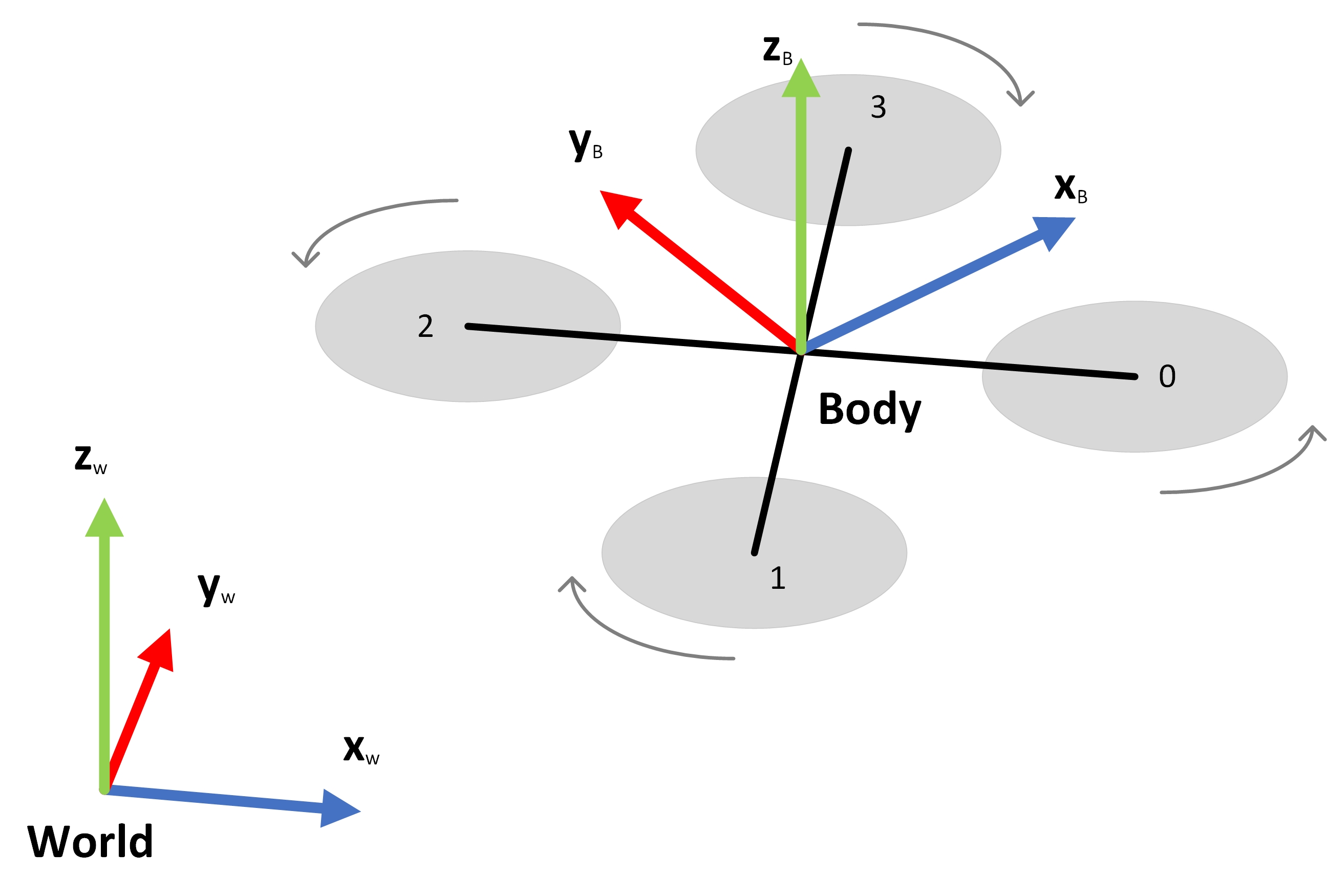
Figure 6: Diagram of the quadrotor the world frame W and the body frame B.

Then we reformulate Equation 14 in its control-affine form:

$$\dot{\bm{x}}=\bm{f}(\bm{x},{\bm{e_{f}}}_{k})+\bm{g}(\bm{x})\bm{u}+\bm{w}$$ (16)

Where $\bm{f}:\mathbb{R}^{n}\mapsto\mathbb{R}^{n}$ and $\bm{g}:\mathbb{R}^{n}\mapsto\mathbb{R}^{n\times m}$ are assumed by the standard as Lipschitz continuous [29, 8]. $\bm{x}=[\bm{P}_{WB},\bm{V}_{WB},\bm{q}_{WB},\bm{\omega}_{B}]^{T}\in\mathbb{X}$, $\bm{u}=T_{i}\forall i\in(0,3)\in\mathbb{U}$ and $\bm{w}\in\mathbb{W}$ are the state, input and additive uncertainty of the dynamic model, where $\mathbb{X}\subseteq\mathbb{R}^{n}$, $\mathbb{U}\subseteq\mathbb{R}^{n_{u}}$ and $\mathbb{W}\subseteq\mathbb{R}^{n_{w}}$ are compact sets as the state, input and uncertainty space, respectively. Given an input $:\mathbb{R}^{\geq 0}\mapsto\mathbb{U}$ and an initial state $x_{0}\in\mathbb{X}$, our goal is to design a quadrotor tracking controller $\bm{u}$ such that the state trajectory $\bm{x}$ can track any reference state trajectory $\bm{x}_{ref}$ (satisfied the quadrotor dynamic limits) under a bounded uncertainty $\bm{w}:\mathbb{R}^{\geq 0}\mapsto\mathbb{W}$.

Appendix C The detailed algorithm of QuaDUE

The objective of this work is to design a distributional-RL-based estimator for CCM uncertainty, which we define as combined wind estimation and CCM uncertainty estimation, for tracking the reference state $\bm{x}_{ref}$ of the nominal model (Equation 14). The detailed algorithm of QuaDUE is shown in Algorithm 1.

Algorithm 1 QuaDUE

Input: $\bm{s}_{k}$, $\bm{s}_{k+1}$, $\bm{u}_{k}$, $\theta^{\mu}$, $\theta^{Q}$
  Output: $\bm{a}_{k}$

1:  Initialize:- $\theta^{\mu^{t}}\leftarrow\theta^{\mu}$, $\theta^{Q^{t}}\leftarrow\theta^{Q}$ update the target parameters from the predicted parameters- the replay memory $D\leftarrow D_{k-1}$- the batch $B$, and its size- a small threshold $\xi\in\mathbb{R_{+}}$ - the random option selection probability $\epsilon$ - the option termination probability $\beta$ - quantile estimation functions $\left\{q_{i}\right\}_{i=1,...,N}$

2:  Repeat

3:  for each sampling step from $D$ do

4:     Select a candidate option $z_{k}$ from $\left\{z^{0},z^{1},...,z^{M}\right\}$

5:     $z_{k}\leftarrow\begin{cases}z_{k-1}&{w.p.\;1-\beta}\\ {\rm{random\;option}}&{w.p.\;\beta\epsilon}\\ {\rm{argmax}}_{z}Q(\bm{s}_{k},z)&{w.p.\;\beta(1-\epsilon)}\end{cases}$

6:     Execute $w_{k}$, get reward $r_{k}$ and the next state $\bm{s}_{k+1}$

7:     $D.\bf{Insert}([\bm{s}_{k},\bm{u}_{k},r_{k},\bm{s}_{k+1}])$

8:     $B\leftarrow D.\bf{sampling}$

9:     $y_{k,i}\leftarrow\rho_{\tau_{i}}^{\mathcal{K}}(r_{k}+\gamma q_{i}^{\prime}(\bm{s}_{k+1},w_{k}^{*})$

10:     $J_{\theta^{\mu}}\leftarrow\frac{1}{N}\sum\limits_{i=1}^{N}\sum\limits_{i^{\prime}=1}^{N}[y_{k,i^{\prime}}-q_{i}(\bm{s}_{k},w_{k})]$

11:     $y\leftarrow\beta{\rm{argmax}}_{z^{\prime}}Q(\bm{s}_{k+1},z^{\prime})+(1-\beta)Q(\bm{s}_{k+1}.z_{k})$

12:     $J_{\theta^{Q}}\leftarrow(r_{t}+\gamma y-Q(\bm{s}_{t},z_{t}))^{2}$

13:     $\theta^{\mu}\leftarrow\theta^{\mu}-l_{\mu}\nabla_{\theta^{\mu}}J_{\theta^{\mu}}$

14:     $\theta^{Q}\leftarrow\theta^{Q}-l_{\theta}\nabla_{\theta^{Q}}J_{\theta^{Q}}$

15:  end for

16:  Until convergence, , $J_{Q}^{\theta}<\xi$

Appendix D The detailed algorithm of Kino-JSS

Quadrotor route searching primarily focuses on robustness, feasibility and efficiency. The Kino-RS algorithm is a robust and feasible online searching approach. However, the searching loop is derived from the hybrid-state A* algorithm, making it relatively inefficient in obstacle-dense environments. On the other hand, JPS offers robust route searching, and runs at an order of magnitude faster than the A* algorithm. A common problem of geometric methods such as JPS and A* is that, unlike kinodynamic searching, they consider heuristic cost (e.g., distance) but not the quadrotor dynamics and feasibility (e.g., line 5 of Algorithm 3 and line 10 of Algorithm 4) when generating routes. $\bf{checkFea()}$ is the feasibility check to judge the acceleration and velocity constrains based on the quadrotor dynamics. Kino-JSS, proposed in [10], generates a safe and efficient route in unknown environments with aerodynamic disturbances. In [10], Kino-JSS, described by Algorithms 2, 3 and 4, is demonstrated to run an order of magnitude faster than Kino-RS [zhou2019robust] in obstacle-dense environments, whilst maintaining comparable system performance.

Algorithm 2 Kinodynamic Jump Space Search

INPUT: $s_{cur}$
OUTPUT: $KinoJSSRoute$

1:  $\bf{initialize()}$

2:  $openSet.\bf{insert(\it{s_{cur}})}$

3:  while !$openSet.\bf{isEmpty()}$ do

4:     $s_{cur}\leftarrow openSet.\bf{pop()}$

5:     $closeSet.\bf{insert(\it{s_{cur}})}$

6:     if $\bf{nearGoal(\it{s_{cur}})}$ then

7:        return  $KinoJSSRoute$

8:     end if

9:     $\bf{KinoJSSRecursion()}$

10:  end while

Algorithm 3 KinoJSSRecursion

INPUT: $s_{cur}$, $E_{f}$, $openSet$, $closeSet$
OUTPUT: $void$

1:  $motions\leftarrow\bf{JSSMotion(\it{s_{cur},E_{f}})}$

2:  for each $m_{i}\in motions$ do

3:     $s_{pro}\leftarrow\bf{statePropagation(\it{s_{cur},m_{i}}))}$

4:     $inClose\leftarrow\it{closeSet}.\bf{isContain(\it{s_{pro}})}$

5:     if $\bf{isFree(\it{s_{pro}})}\bigwedge\bf{checkFea(\it{s_{pro},m_{i}})}\bigwedge\it{inClose}$ then

6:        if  $\bf{checkOccupiedAround(\it{s_{pro}})}$ then

7:           $s_{pro}.neighbors\leftarrow\bf{JSSNeighbor(\it{s_{pro}})}$

8:           $cost_{pro}\leftarrow\it{s_{cur}}.cost+\bf{edgeCost(\it{s_{pro}})}$

9:           $cost_{pro}\leftarrow cost_{pro}+\bf{heuristic(\it{s_{pro}})}$

10:           if !$\it{openSet}.\bf{isContain(\it{s_{pro}})}$ then

11:              $openSet.\bf{insert(\it{s_{pro}})}$

12:           else if $\it{s_{pro}}.cost\leq\it{cost_{pro}}$ then

13:              continue

14:           end if

15:           $s_{pro}.parent\leftarrow s_{cur}$

16:           $s_{pro}.cost\leftarrow cost_{pro}$

17:        else

18:           $\bf{KinoJSSRecursion()}$

19:        end if

20:     else

21:        continue

22:     end if

23:  end for

Algorithm 4 JSSMotion

INPUT: $s_{cur}$, $E_{f}$
OUTPUT: $motions$

1:  $E_{fcor}\leftarrow E_{f}+\bf{GaussianNoise()}$

2:  for each $m_{i}\in motionSet$ do

3:     $m_{cor}\leftarrow m_{i}+E_{fcor}$

4:     $motions\leftarrow\bf{push\_back(\it{m_{cor}})}$

5:  end for

6:  $neighSize\leftarrow s_{cur}.neighbors.\bf{size()}$

7:  while $neighSize\neq 0$ do

8:     $neighSize=neighSize-1$

9:     $neighMotion\leftarrow\bf{posToMotion(\it{s_{cur}.neighbors)}}$

10:     if $\bf{checkFea(\it{s_{cur},neighMotion})}$ then

11:        $motions\leftarrow\bf{push\_back(\it{neighMotion})}$

12:     end if

13:  end while

14:  return  $motions$

$s_{cur}$ denotes the current state, $s_{pro}$ denotes the propagation of current state under the motion $m_{i}$, and $E_{f}$ denotes the aerodynamic disturbance estimated by VID-fusion [36]. In Algorithm 2, $\bf{JSSNeighbor()}$ is defined as shown in Fig. 8. In Algorithm 3, $motionSet$, which is defined as a pyramid shown in Fig. 9, offers improved efficiency whilst retaining the advantages of Kino-RS [zhou2019robust]. As shown in Figure 7, the experiments with 499, 249 and 149 obstacles demonstrate the Kino-JSS’s performance in environments of varying obstacle-density.

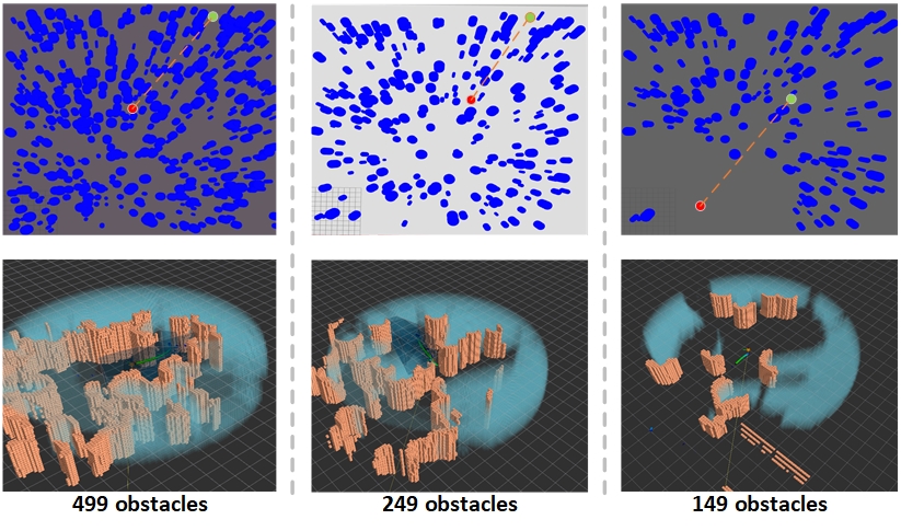
Figure 7: Three kinds of environment with different obstacles (499, 249 and 149 obstacles) in the simulation.

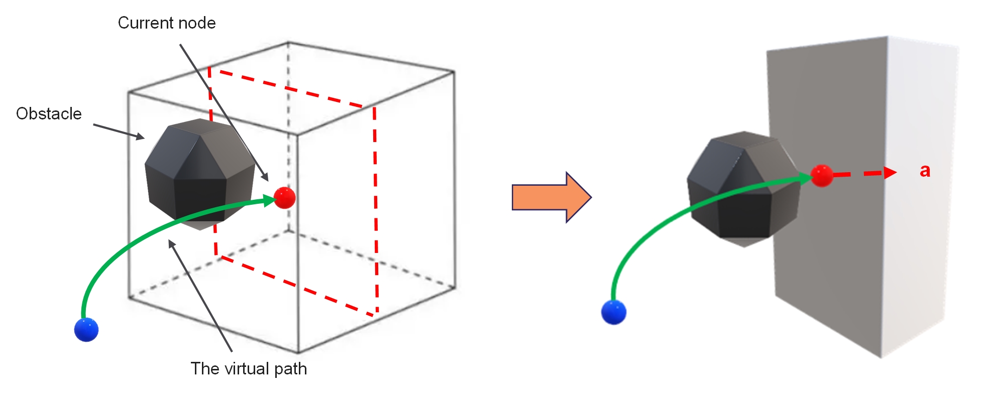
Figure 8: Diagram of KinoJSS when checking occupied obstacles around: a grey cuboid is generated as the ‘forced neighbour’, the output of $\bf{JSSNeighbor()}$, in Algorithm 2.

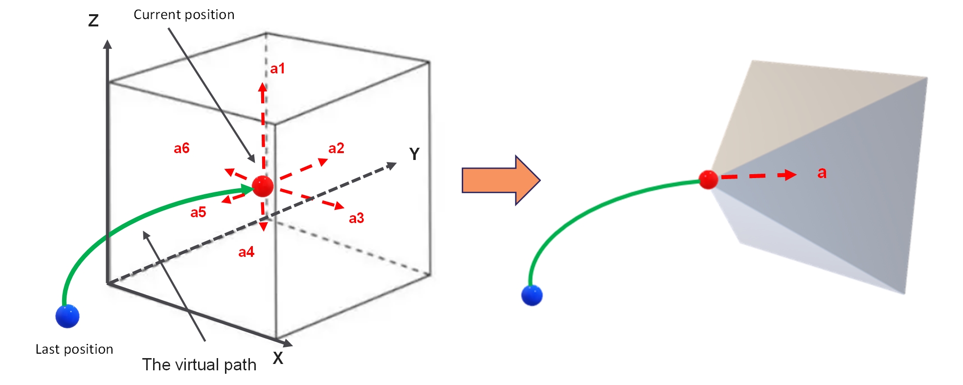
Figure 9: Diagram of KinoJSS with unoccupied space around: the pyramid represents the $motionSet$ in Algorithm 3, i.e., $\bf{JSSMotion()}$, in free space.

Appendix E The implementation details of QuaDUE-CCM

Table 3: Parameters of QuaDUE-CCM

Parameters	Definition	Values
$l_{\theta_{a}}$	Learning rate of actor	0.001
$l_{\theta_{c}}$	Learning rate of critic	0.001
$\theta_{a}$	Actor neural network: fully connected with two hidden layers (128 neurons per hidden layer)	-
$\theta_{c}$	Critic neural network: fully connected with two hidden layers (128 neurons per hidden layer)	-
$D$	Replay memory capacity	$10^{6}$
$B$	Batch size	256
$\gamma$	Discount rate	0.998
-	Training episodes	1000
$T_{s}$	MPC Sampling period	50ms
$N$	Time steps	20

We evaluate the performance of our proposed QuaDUE-CCM framework, in which a DJI Manifold 2-C (Intel i7-8550U CPU) is used for real-time computation. We use RotorS MAVs simulator [43], in which programmable aerodynamic disturbances can be generated, for testing the QuaDUE-CCM framework. The nominal force $\bm{n_{f}}$ is estimated by VID-Fusion [36]. The noise bound of aerodynamic forces is set as 0.5 $m/s^{2}$, based on the benchmark established in [44]. Since the update frequency of the aerodynamic force $\bm{e_{f}}$ estimation is much higher than our QuaDUE-CCM framework frequency, we sample $\bm{e_{f}}$ based on our framework frequency. We also assume the collective thrust $\bm{c}$ is a true value, which is tracked ideally in the simulation platform.

The parameters of our proposed framework are summarized in Table 3. Then we operate a training process by generating external forces in RotorS [43], where the programmable external forces are in the horizontal plane with range [-3,3] ($m/s^{2}$). The training process has 1000 iterations where the quadrotor state is recorded at 16 $Hz$. The training process is occurs over 1000 iterations. The matrices $H_{1}$ and $H_{2}$ in Equation 10 are chosen as $H_{1}=diag\{2.5e^{-2},2.5e^{-2},2.5e^{-2},1e^{-3},1e^{-3},1e^{-3},2.5e^{-3},2.5e^{-3},2.5e^{-3},2.5e^{-3},1e^{-5},1e^{-5},1e^{-5}\}$ and $H_{2}=diag\{1.25e^{-4},1.25e^{-4},1.25e^{-4},1.25e^{-4}\}$, respectively.

References

- Torrente et al. [2021] G. Torrente, E. Kaufmann, P. Föhn, and D. Scaramuzza. Data-driven mpc for quadrotors. IEEE Robotics and Automation Letters, 6(2):3769–3776, 2021.
- Faessler et al. [2017] M. Faessler, A. Franchi, and D. Scaramuzza. Differential flatness of quadrotor dynamics subject to rotor drag for accurate tracking of high-speed trajectories. IEEE Robotics and Automation Letters, 3(2):620–626, 2017.
- Hoffmann et al. [2007] G. Hoffmann, H. Huang, S. Waslander, and C. Tomlin. Quadrotor helicopter flight dynamics and control: Theory and experiment. In AIAA guidance, navigation and control conference and exhibit, page 6461, 2007.
- Russell et al. [2016] C. R. Russell, J. Jung, G. Willink, and B. Glasner. Wind tunnel and hover performance test results for multicopter uas vehicles. In American Helicopter Society (AHS) International Annual Forum and Technology Display, number ARC-E-DAA-TN31096, 2016.
- Kaya and Kutay [2014] D. Kaya and A. T. Kutay. Aerodynamic modeling and parameter estimation of a quadrotor helicopter. In AIAA Atmospheric Flight Mechanics Conference, page 2558, 2014.
- Bellemare et al. [2017] M. G. Bellemare, W. Dabney, and R. Munos. A distributional perspective on reinforcement learning. In International Conference on Machine Learning, pages 449–458. PMLR, 2017.
- Lohmiller and Slotine [1998] W. Lohmiller and J.-J. E. Slotine. On contraction analysis for non-linear systems. Automatica, 34(6):683–696, 1998.
- Dawson et al. [2022] C. Dawson, S. Gao, and C. Fan. Safe control with learned certificates: A survey of neural lyapunov, barrier, and contraction methods. arXiv preprint arXiv:2202.11762, 2022.
- Lillicrap et al. [2015] T. P. Lillicrap, J. J. Hunt, A. Pritzel, N. Heess, T. Erez, Y. Tassa, D. Silver, and D. Wierstra. Continuous control with deep reinforcement learning. arXiv preprint arXiv:1509.02971, 2015.
- Wang et al. [2022] Y. Wang, J. O’Keeffe, Q. Qian, and D. E. Boyle. Kinojgm: A framework for efficient and accurate quadrotor trajectory generation and tracking in dynamic environments. In 2022 IEEE International Conference on Robotics and Automation (ICRA) [to appear]. IEEE, 2022.
- Spielberg et al. [2021] N. A. Spielberg, M. Brown, and J. C. Gerdes. Neural network model predictive motion control applied to automated driving with unknown friction. IEEE Transactions on Control Systems Technology, 2021.
- Salzmann et al. [2022] T. Salzmann, E. Kaufmann, M. Pavone, D. Scaramuzza, and M. Ryll. Neural-mpc: Deep learning model predictive control for quadrotors and agile robotic platforms. arXiv preprint arXiv:2203.07747, 2022.
- Loquercio et al. [2021] A. Loquercio, E. Kaufmann, R. Ranftl, M. Müller, V. Koltun, and D. Scaramuzza. Learning high-speed flight in the wild. Science Robotics, 6(59):eabg5810, 2021.
- Wang et al. [2022] Y. Wang, J. O’Keeffe, Q. Qian, and D. Boyle. Interpretable stochastic model predictive control using distributional reinforced estimation for quadrotor tracking systems. arXiv preprint arXiv:2205.07150, 2022.
- Zhang et al. [2021] Q. Zhang, W. Pan, and V. Reppa. Model-reference reinforcement learning for collision-free tracking control of autonomous surface vehicles. IEEE Transactions on Intelligent Transportation Systems, 2021.
- Ma et al. [2021] Y. Ma, D. Jayaraman, and O. Bastani. Conservative offline distributional reinforcement learning. Advances in Neural Information Processing Systems, 34, 2021.
- Sun et al. [2021] K. Sun, Y. Zhao, Y. Liu, E. Shi, Y. Wang, A. Sadeghi, X. Yan, B. Jiang, and L. Kong. Towards understanding distributional reinforcement learning: Regularization, optimization, acceleration and sinkhorn algorithm. arXiv preprint arXiv:2110.03155, 2021.
- Jha et al. [2018] S. Jha, S. Raj, S. K. Jha, and N. Shankar. Duality-based nested controller synthesis from stl specifications for stochastic linear systems. In International Conference on Formal Modeling and Analysis of Timed Systems, pages 235–251. Springer, 2018.
- Khalil [2015] H. K. Khalil. Nonlinear control, volume 406. Pearson New York, 2015.
- Ames et al. [2016] A. D. Ames, X. Xu, J. W. Grizzle, and P. Tabuada. Control barrier function based quadratic programs for safety critical systems. IEEE Transactions on Automatic Control, 62(8):3861–3876, 2016.
- Singh et al. [2019] S. Singh, B. Landry, A. Majumdar, J.-J. Slotine, and M. Pavone. Robust feedback motion planning via contraction theory. The International Journal of Robotics Research, 2019.
- Tsukamoto and Chung [2020] H. Tsukamoto and S.-J. Chung. Neural contraction metrics for robust estimation and control: A convex optimization approach. IEEE Control Systems Letters, 5(1):211–216, 2020.
- Tsukamoto et al. [2020] H. Tsukamoto, S.-J. Chung, and J.-J. E. Slotine. Neural stochastic contraction metrics for learning-based control and estimation. IEEE Control Systems Letters, 5(5):1825–1830, 2020.
- Qin et al. [2021] Z. Qin, K. Zhang, Y. Chen, J. Chen, and C. Fan. Learning safe multi-agent control with decentralized neural barrier certificates. arXiv preprint arXiv:2101.05436, 2021.
- Qin et al. [2022] Z. Qin, D. Sun, and C. Fan. Sablas: Learning safe control for black-box dynamical systems. IEEE Robotics and Automation Letters, 7(2):1928–1935, 2022.
- Chang and Gao [2021] Y.-C. Chang and S. Gao. Stabilizing neural control using self-learned almost lyapunov critics. In 2021 IEEE International Conference on Robotics and Automation (ICRA), pages 1803–1809. IEEE, 2021.
- Kamel et al. [2017] M. Kamel, T. Stastny, K. Alexis, and R. Siegwart. Model predictive control for trajectory tracking of unmanned aerial vehicles using robot operating system. In Robot operating system (ROS), pages 3–39. Springer, 2017.
- Falanga et al. [2018] D. Falanga, P. Foehn, P. Lu, and D. Scaramuzza. Pampc: Perception-aware model predictive control for quadrotors. In 2018 IEEE/RSJ International Conference on Intelligent Robots and Systems (IROS), pages 1–8. IEEE, 2018.
- Choi et al. [2020] J. Choi, F. Castaneda, C. J. Tomlin, and K. Sreenath. Reinforcement learning for safety-critical control under model uncertainty, using control lyapunov functions and control barrier functions. arXiv preprint arXiv:2004.07584, 2020.
- Dawson et al. [2022] C. Dawson, B. Lowenkamp, D. Goff, and C. Fan. Learning safe, generalizable perception-based hybrid control with certificates. IEEE Robotics and Automation Letters, 2022.
- Sun et al. [2020] D. Sun, S. Jha, and C. Fan. Learning certified control using contraction metric. arXiv preprint arXiv:2011.12569, 2020.
- Manchester and Slotine [2017] I. R. Manchester and J.-J. E. Slotine. Control contraction metrics: Convex and intrinsic criteria for nonlinear feedback design. IEEE Transactions on Automatic Control, 62(6):3046–3053, 2017.
- Tsukamoto and Chung [2020] H. Tsukamoto and S.-J. Chung. Robust controller design for stochastic nonlinear systems via convex optimization. IEEE Transactions on Automatic Control, 66(10):4731–4746, 2020.
- Zhao et al. [2022] P. Zhao, A. Lakshmanan, K. Ackerman, A. Gahlawat, M. Pavone, and N. Hovakimyan. Tube-certified trajectory tracking for nonlinear systems with robust control contraction metrics. IEEE Robotics and Automation Letters, 7(2):5528–5535, 2022.
- Gallot et al. [1990] S. Gallot, D. Hulin, and J. Lafontaine. Riemannian geometry, volume 2. Springer, 1990.
- Ding et al. [2020] Z. Ding, T. Yang, K. Zhang, C. Xu, and F. Gao. Vid-fusion: Robust visual-inertial-dynamics odometry for accurate external force estimation. arXiv preprint arXiv:2011.03993, 2020.
- Puterman [2014] M. L. Puterman. Markov decision processes: discrete stochastic dynamic programming. John Wiley & Sons, 2014.
- Dabney et al. [2018] W. Dabney, M. Rowland, M. Bellemare, and R. Munos. Distributional reinforcement learning with quantile regression. In Proceedings of the AAAI Conference on Artificial Intelligence, volume 32, 2018.
- Andersson et al. [2019] J. A. Andersson, J. Gillis, G. Horn, J. B. Rawlings, and M. Diehl. Casadi: a software framework for nonlinear optimization and optimal control. Mathematical Programming Computation, 11(1):1–36, 2019.
- Verschueren et al. [2018] R. Verschueren, G. Frison, D. Kouzoupis, N. van Duijkeren, A. Zanelli, R. Quirynen, and M. Diehl. Towards a modular software package for embedded optimization. IFAC-PapersOnLine, 51(20):374–380, 2018.
- Joyce [2011] J. M. Joyce. Kullback-leibler divergence. In International encyclopedia of statistical science, pages 720–722. Springer, 2011.
- Zhang and Yao [2019] S. Zhang and H. Yao. Quota: The quantile option architecture for reinforcement learning. In Proceedings of the AAAI Conference on Artificial Intelligence, volume 33, pages 5797–5804, 2019.
- Furrer et al. [2016] F. Furrer, M. Burri, M. Achtelik, and R. Siegwart. Rotors—a modular gazebo mav simulator framework. In Robot operating system (ROS), pages 595–625. Springer, 2016.
- Wu et al. [2021] Y. Wu, Z. Ding, C. Xu, and F. Gao. External forces resilient safe motion planning for quadrotor. IEEE Robotics and Automation Letters, 6(4):8506–8513, 2021.