ESFPNet: efficient deep learning architecture for real-time lesion segmentation in autofluorescence bronchoscopic video

Abstract

Lung cancer tends to be detected at an advanced stage, resulting in a high patient mortality rate. Thus, much recent research has focused on early disease detection. Lung cancer generally first appears as lesions developing within the bronchial epithelium of the airway walls. Bronchoscopy is the procedure of choice for effective noninvasive bronchial lesion detection. In particular, autofluorescence bronchoscopy (AFB) discriminates the autofluorescence properties of normal and diseased tissue, whereby lesions appear reddish brown in AFB video frames, while normal tissue appears green. Because recent studies show AFB’s high sensitivity for lesion detection, it has become a potentially pivotal method during the standard bronchoscopic airway exam for early-stage lung cancer detection. Unfortunately, manual inspection of AFB video is extremely tedious and error prone, while limited effort has been expended toward potentially more robust automatic AFB lesion detection and segmentation. We propose a real-time deep-learning architecture dubbed ESFPNet for accurate segmentation and robust detection of bronchial lesions in an AFB video stream. The architecture features an encoder structure that exploits pretrained Mix Transformer (MiT) encoders and an efficient stage-wise feature pyramid (ESFP) decoder structure. Segmentation results derived from the AFB airway-exam videos of 20 lung cancer patients indicate that our approach gives a mean Dice index = 0.756 and average Intersection of Union = 0.624, results that are superior to those generated by other recent architectures. In addition, our method enables a processing throughput of 27 frames/sec. Thus, ESFPNet gives the physician a potential tool for confident real-time lesion segmentation and detection during a live bronchoscopic airway exam. Moreover, our model shows promising potential applicability to other domains, as evidenced by its state-of-the-art (SOTA) performance on the CVC-ClinicDB and ETIS-LaribPolypDB datasets and its superior performance on the Kvasir and CVC-ColonDB datasets.

1 INTRODUCTION

Lung cancer is the most common cause of cancer death worldwide [1]. An important goal toward improving lung cancer survival is to detect the disease at an early stage, thereby giving an opportunity for the most effective treatment options. Lung cancer begins when lesions develop in the bronchial epithelium of the lung mucosa. These bronchial lesions, which can eventually evolve into squamous cell lung cancer, also help predict the potential development of other lung cancers. Hence, methods for early detection of bronchial lesions are essential to help improve lung cancer patient care. A noninvasive way for physicians to search for such lesions is to use bronchoscopy for imaging the airway epithelium during a routine airway exam [2]. Among the current advanced videobronchosopic techniques, autofluorescence bronchoscopy (AFB) exhibits high sensitivity to suspicious bronchial lesions and effectively distinguishes developing bronchial lesions from the normal epithelium. In AFB video, lesions appear reddish brown, while normal tissue appears green. Unfortunately, current standard practice entails manual inspection of an incoming AFB video stream, which is extremely tedious and error prone.

A promising strategy for improving this situation is to consider computer-based lesion analysis methods for AFB video frames. A simple, but largely ineffective, approach applied in some clinical work is to measure the red/green ratio [3]. Other more recent work has considered standard computer-based image processing methods and/or conventional machine learning techniques [4, 5, 6]: Unfortunately, these works all have at least one of the following limitations:

1. Need complicated image preprocessing, including image enhancement and/or feature extraction before reaching lesion decisions.

2. Do not provide robust, accurate segmentation of abnormal lesion regions as an aid toward locating potential lesions.

3. Can’t process an input AFB video stream in real-time, thereby making the methods unsuitable for making lesion decisions during a live bronchoscopic airway exam.

These limitations make the methods unsuitable for lesion segmentation and detection during a live bronchoscopic airway exam.

Recent deep-learning-based architectures, which have achieved great success in medical image analysis, show much promise for handling these limitations. As an example, Unet++ is a powerful and widely used architecture for semantic medical image segmentation [7]. The Unet++ adds efficient and densely-connected nested-decoder subnetworks to the popular Unet architecture.[8] It also applies a deep supervision mechanism that allows for improved aggregation of features across different semantic scales. Although Unet++ can provide more accurate segmentations than Unet, the requisite dense connections demand extensive computation.

As another example, the Caranet also utilizes deep supervision to enhance the use of aggregative features [9]. Yet, in contrast to the complicated sub-networks of Unet++, the Caranet includes the advantageous self-attention mechanism and draws on the context axial reverse attention technique on a pretrained Res2Net backbone. Hence, it has been shown to enable faster processing time and better segmentation performance than Unet++ when tested over multiple public medical datasets. Nevertheless, the design of the self-attention mechanism in the Caranet is complex. On another front, the Segformer has shown much success in the semantic segmentation domain [10]. The Segformer provides a simple and efficient layout that utilizes the attention technique referred to as “Mix Transformer (MiT) encoders.” In a later development, the SSFormer architecture extracts aggregate local and global step-wise features from pretrained MiT encoders to predict abnormal regions [11]. Tests with the CVC-ColonDB and Kvasir-SEG datasets demonstrate the generalizability and superior performance of the SSFormer (and its use of the MiT encoders) over Caranet for medical imaging applications. Yet, the feature pyramid used by SSFormer could be made more efficient, thereby reducing the processing time and network complexity. Note that the number of parameters defining a network gives a direct indication of the number of floating-point operations (FLOPS) needed to process an input and, hence, its computational efficiency (execution time). (Table 2 later illustrates this point.)

We propose a more efficient deep-learning-based architecture that enables real-time segmentation and detection of bronchial lesions in an AFB video. Our architecture draws on pretrained Mix Transformer (MiT) encoders as the backbone and a decoder structure that incorporates an efficient stage-wise feature pyramid (ESFP) to help promote accurate lesion segmentation.

2 METHODS

For a given AFB video sequence, our goal is achieve both high lesion detection accuracy and high computational throughput. At the outset, we point out that state-of-the-art deep-learning-based neural network architectures generally require a large amount of data to adequately train and test them (the “data hunger” problem). This is because of the large number of network parameters that require precise tuning during the training process. Unfortunately, for our AFB video analysis application, while we seemingly have a large dataset available to training and testing, the amount of data we have still proves to be insufficient. Our proposed approach offers a solution to all of these issues.

Figure 1 depicts the proposed ESFPNet architecture, which utilizes the Mix Transformer (MiT) encoder as the backbone and uses an efficient stage-wise feature pyramid (ESFP) as the decoder to generate segmentation outputs. The basic input is a raw AFB video frame, while the output is a frame that either presents a segmented detected lesion or no output (a normal frame).

Sections 2.1-2.2 describe each component of the architecture. Section 2.3 then discusses implementation details.

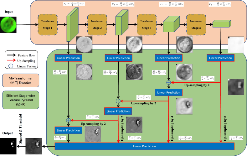
Figure 1: Block diagram of the ESPFNet architecture.

2.1 Backbone

CNN-based encoders, such as the Unet and SegNet implementations, have enjoyed much success for image segmentation tasks (CNN = convolutional neural network) [8, 12]. A CNN-based encoder, motivated by the idea that every image pixel depends on its neighboring pixels, uses filters on an image patch to extract relevant local features. Yet, if a processing model utilized all image data instead of only the patches considered by the filters, then processing performance would be expected to improve. This concept helps the so-called Vision Transformers (ViT) work better than most CNN models [13]. The Mix Transformer encoder (MiT) is a module that takes advantage of the idea of the ViT network and uses four overlapping path-merging modules and self-attention prediction in four stages [10]. These stages not only furnish high-resolution coarse features, but also provide low-resolution fine-grained features. In addition, the high- and low-resolution features are commonly used to boost the performance of semantic segmentation.

On the other hand, the limitation of using transformers as encoders is obvious. The self-attention layers used by transformers lack locality inductive bias (the notion that image pixels are locally correlated and that their correlation maps are translation-invariant) and lead to the problem of data hunger [13]. To alleviate the challenge of data hunger for applications limited by small datasets, one can exploit the widely used concept of transfer learning. The MiT encoders, which take advantage of this idea, are pretrained on the large ImageNet database [14]. For our ESPFNet architecture, we integrate these pretrained MiT encoders as our backbone and train them again with the initialized decoders. This proves to be a straightforward way to facilitate good performance over our small task-specific datasets, while also being able to exceed the performance of state-of-the-art CNN models.

2.2 Efficient stage-wise feature pyramid (ESFP)

The prediction results of the decoder rely on multi-level features from the encoder, where local (low-level) features are extracted from the shallow parts of the encoders, while global (high-level) features are extracted from the deeper parts. Previous research has demonstrated that the sufficiency of local features obtained in the shallow part of the transformer directly affects the model’s performance [15]. The existing Segformer model, however, equally concatenates these multi-level features to predict segmentation results and, hence, lacks the ability to sufficiently and selectively use the local features [10]. To address this issue, the SSFormer architecture includes an aggregating feature pyramid architecture that first utilizes two layers of convolution to preprocess feature outputs from each MiT stage. It then fuses any two features in reverse order (from deep to shallow) until final prediction [11]. In this way, local features gradually guide the model’s attention to critical regions.

We point out, however, that high-level (global) features contribute more to overall segmentation performance than low-level (local) features. Although SSFormer enhances the contribution of local features, the usage of high-level features is weakened. Furthermore, the SSFormer architecture’s usage of the two convolution layers is inefficient. Inspired by the structure of a lightweight channel-wise feature pyramid network (CfpNet) that fuses every pair of features and concatenates multi-level fused elements for the final prediction, we propose a novel and efficient stage-wise feature pyramid (ESFP) to exploit multi-stage features [16]. ESFP starts with linear predictions of each stage output (efficient in the number of connecting channels) and then linearly fuses these preprocessed features from global to local. These intermediate aggregating features are concatenated and work cooperatively to produce final segmentations.

As a final comment, we tested several different versions of the proposed ESFPNet architecture based of the different MiT encoder scales available [10]: ESFPNet-T (tiny model), ESFPNet-S (standard model), and ESFPNet-L (large model), which are based on the MiT-B0, -B2, and -B4 encoders, respectively.

2.3 Implementation details

We implemented our model in Pytorch and accelerated training via NVIDIA GPUs. Given the difference in MiT encoders’ scales and the GPU memory required to train, we trained these networks either on an NVIDIA RTX 3090 or on an NVIDIA TESLA A100 GPU. Before training, we resized the inputs to $352\times 352$ pixels and normalized them for segmentation. We also employed random flipping, rotation, and brightness changing as data augmentation operations on the inputs. Our loss function combines the weighted intersection over union (IoU) loss and the weighted binary cross-entropy (BCE) loss:

$$L=L^{w}_{\rm IoU}+L^{w}_{\rm BCE}\ .$$ (1)

We used the default AdamW optimizer with the learning rate $1e^{-4}$ and trained our models for 200 epochs.

Details for the training and validation data sets appear in Section 3. Next, Section 4 gives a series of experiments that not only measure the performance of our proposed ESFPNET model, but also compares it to other recent deep learning models.

3 Experimental Datasets and Metrics

This section summarizes the test datasets and validation metrics used for the experiments. Section 3.1 summarizes our AFB dataset. As an additional validation experiment to measure our network’s general applicability to other domains, we also performed tests with five public datasets, as summarized in Section 3.2: Kvasir[17], CVC-ClinicDB[18], CVC-T[19], CVC-ColonDB[20], and ETIS-LaribPolypDB[21]. Finally, Section 3.3 discusses the test metrics employed.

3.1 AFB image dataset

Table 1 summarizes the details of our AFB image dataset. For our dataset, we isolated 208 lesion frames (frame size, $720\times 720$), which depicted clear ground truth bronchial lesions, and also selected 477 normal frames. These frames were drawn from the AFB airway exams from 20 lung cancer patients seen at our University Hospital. These cases were collected under informed consent and an approved IRB protocol. Because a lesion typically appears in many frames within a given video sequence, we selected Lesion frames to ensure variations in airway location, size, and viewing direction. Also, all frames were labeled by an expert. Regarding the normal frames, we selected these randomly around the vicinity of each observed airway bifurcation, taking care not involve any lesions or lesion components in selected frames.

As Table 1 shows, we split the AFB dataset into train, test, and validation subsets using approximately a 50%, 25%, and 25% split, respectively. Every lesion and normal frame from a given case was placed in the same subset to guarantee independence between training, testing, and validation phases. Lastly, the lesion sizes summarized in Table 1 are given as percentages, where 100% = 352$\times$352$\times\pi$ pixels (this is the pixel-based area of an AFB frame’s circular scan region).

Dataset	case / (lesion frames, normal frames)	total lesion / normal frames	lesion/normal split ratio	lesion size range
Train	156 / (35,16); 176 / (8,24); 178 / (7,17); 192 / (19,24); 188 / (12,11); 172 / (0,39); 189 / (0,30); 191 / (0,26); 182 / (5,22); 187 / (11,14)	97 / 223	46.7% / 46.8%	0.31% - 54.30%
Validation	171 / (58,3); 181 / (0,43); 173 / (0,35); 179 / (0,35); 180 / (0,23)	58 / 139	27.9% / 27.1%	0.20% - 75.15%
Test	184 / (33,3); 174 / (9,25); 195 / (11,16); 157 / (0,35); 190 / (0,36)	53 / 115	25.4% / 24.1%	0.47% - 45.87%

Table 1: AFB dataset details. “case” = patient case number, “lesion/normal frames” = the number of lesion or normal frames selected from a case, “total lesion/normal frames” = the total number of selected lesion or normal frames for a particular data subset, while “lesion/normal split ratio” gives the percentage of frames in a given class (lesion or normal) assigned to a particular data subset. Finally, “lesion size range” indicates the range of lesion sizes encountered in a particular subset, where the values indicate what percent of a frame’s circular scan area contains a lesion.

In addition, Figure 2 gives sample frames in the training and validation dataset that illustrate the variations in lesion size ratio. Each frame pair gives the original frame (left) and ground truth segmentation (right). As one looks from left to right in the figure, lesion size increases. We note in passing that the lesion size ratio in the validation dataset is broader than for the training dataset. Note that our dataset often draws on multiple frames depicting the same lesion area. Yet, these frames show very different appearances of the lesion, because of inter-frame variations in viewing direction and distance. For instance, the first two pairs in Figure 2 correspond to same lesion appearing in the left lower lobe of patient case 171: the second pair is captured from a position closer to the lesion than the first pair.

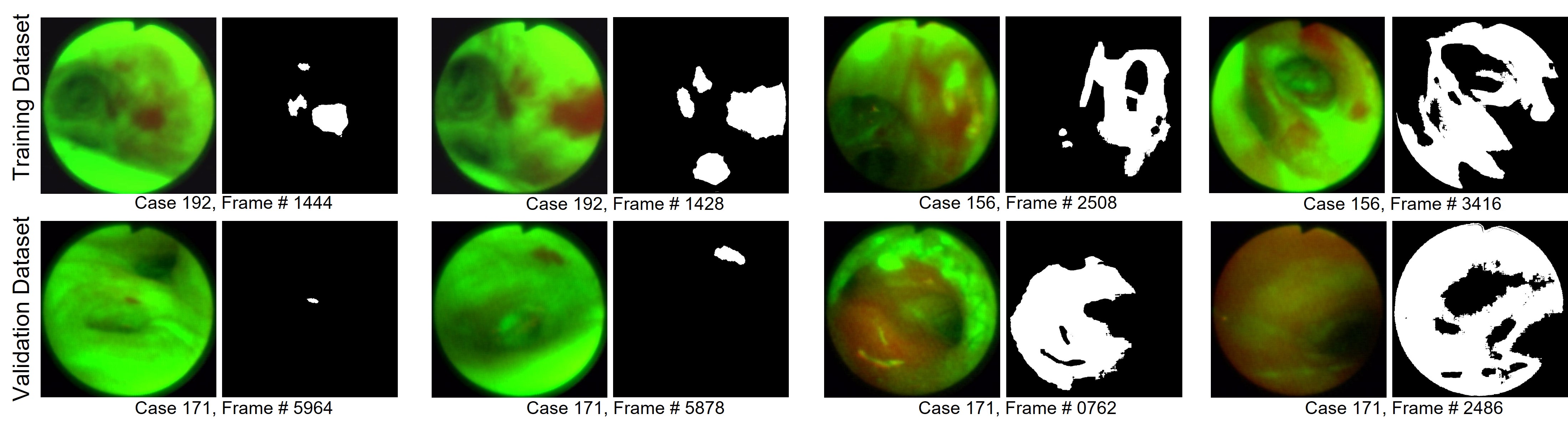
Figure 2: AFB lesion examples from four cases: two from the training subset (first row) and two from the validation subset (second row). Each frame pair gives the original frame (left) and ground truth lesion segmentation (right). Note that the lesions contained in these frames increase in size left to right in each row. Lastly, for each row, the first two image pairs (row 1: case 192; row 2: case 171) correspond to the same lesion observed from different bronchoscope viewing positions.

3.2 Polyp segmentation datasets

An effective image pattern-recognition model ideally exhibits strong capabilities for learning and generalizability. In particular, if a model is trained with a particular dataset, then the model’s learning ability indicates its prediction accuracy. Similarly, generalizability refers to a model’s ability to adapt to previously unseen datasets. To ascertain the EPFSNet model’s learning capabilities and generalizability, in Section 4.2, we compare our ESFPNet to several state-of-the-art medical image-segmentation models: Unet++[7], Deeplabv3+[22], SFA[23], CaraNet[9], MSRF-Net[24], and SSFormer[11]. In particular, for these datasets, we set up three additional experiments summarized below.

Learning ability experiment: Following the experimental scheme of MSRF-Net[24], we train, validate, and test ESFPNet on the Kavsir and CVC-ClinicDB benchmark datasets. We randomly split each dataset into three subsets: 80$\%$ training, 10$\%$ validation, and 10$\%$ test. We freeze the model when it reaches the optimized dice coefficient on the validation dataset. We then use the frozen model to generate prediction results for the test dataset.

Generalizability experiment: We use the same dataset splitting as recommended in the experimental scheme of ParaNet[25], which used 1450 (90$\%$) video frames from the Kvasir and CVC-ClinicDB datasets for training. All images from CVC-ColonDB and ETIS-LaribPolypDB are used for testing. We keep the best attained performance for each dataset as measures of a model’s forecasting performance on an unseen dataset.

Power balance experiment: We use the same training dataset as in the generalizability experiment. The remaining frames from the Kvasir and CVC-ClinicDB datasets and all images from CVC-ColonDB, CVC-T, and ETIS-LaribPolypDB are used for testing. A model is frozen when it reaches convergence and later utilized in the testing phase to analyze the segmentation performance over 5 test datasets.

3.3 Baseline and measurement metrics

To evaluate our results, we use the following metrics: mean dice; mean IoU; structural measurement $S_{\alpha}$[26]; enhanced alignment metric $E_{\phi}^{max}$[27]; and the average mean absolute error (MAE), which gives a measure of pixel-level accuracy. In addition, we use $S_{\alpha}$ to measure the structural similarity between predictions and ground truth and the recently proposed $E_{\phi}^{max}$ to assess both the pixel-level and global-level similarity. We computed all metrics using the freely available ParaNet tool [25]. When making comparisons to other models, we only use mean dice and mean IoU as the unifying measures in the learning ability and the power balance experiments.

4 RESULTS

4.1 AFB dataset experiments

We trained ESFPNet-T, ESFPNet-S, and ESFPNet-L on our AFB dataset with batch size 16. Since the number of lesion and normal frames is not balanced, we added weights on these two classes to the sampler to guarantee balance when sampling a batch. We also trained the Unet++ , SSFormer-S, SSFormer-L, and CARANet models under the same conditions [7, 11, 9]. Lastly, results for the R/G method and previously tested machine learning method are given by Chang et al. [6]. Table 2 gives the quantitative comparison between various methods. To help assess a model’s complexity and processing time, the table also lists two attributes of the various models: number parameters in a model and the amount of computation (number of floating-point operations) required to derive an output.

Among the various analysis methods, only R/G analysis and our previously proposed machine learning method missed lesion frames; also these two approaches gave the largest number of frames falsely identified as lesion frames. Overall, our proposed ESFPNet-S model achieved the best segmentation results, while utilizing the third-fewest network parameters and giving the second fastest execution time. Although Unet++ requires the second fewest parameters, it generated 5 FP frames. No other deep learning network gave any FN or FP frames. Notably, ESFPNet-S uses the same backbone as the SSFormer-S. Yet, it performs better in terms of the mDice and mIoU indices while also requiring fewer GFLOPs for computation SSFormer-S. These same results also when comparing ESFPNet-L to SSFormer-L. The CaraNet and SSFormer-S give nearly identical results, yet CaraNet requires more parameters and computation than either SSFormer-S or ESFPNet-S. Overall, ESFPNet-S appears to offer the best balance between analysis performance and architectural efficiency for the AFB dataset.

	Architecture Attribute		AFB Results
Architecture	Parameters	GFLOPs	Mean Dice	Mean IoU	FN Frames	FP Frames
Masked R/G	N/A	N/A	0.549	0.418	5	10
SVM-EMBC	N/A	N/A	0.329	0.219	1	26
ESFPNet-T (B0)	3.5	1.4	0.717	0.574	0	0
ESFPNet-S (B2)	25.0	9.3	0.756	0.624	0	0
SSFormer-S (B2)	29.6	20.0	0.746	0.612	0	0
ESFPNet-L (B4)	61.7	23.9	0.738	0.600	0	0
SSFormer-L (B4)	66.2	34.6	0.737	0.604	0	0
Unet++	9.2	65.7	0.722	0.587	0	5
CaraNet	46.6	21.8	0.745	0.610	0	0

Table 2: AFB experimental results. “Parameters” = number of architecture parameters in millions, GFLOPs = gigaflops (flops = floating-point operations). The GFLOPs count assumes input dimensions = (1,3,352,352). FN = frame is misclassified as a normal frame, but is actually a lesion frame (false negative). FP = frame is misclassified as a lesion frame, but is actually a normal frame (false positive). FN and FP results are over 53 lesion and 115 normal frames, respectively. “SVM” refers to a machine learning method proposed previously by Chang et al. [6]. “N/A” = not applicable. BOLD numbers indicate the best measures.

Figure 3 depicts sample AFB segmentation results. These results organized in order of the best segmentation results (by ESPFNet-S) to the worst (by SVM-EMBC); this order also reflects decreasing mDice and mIoU values. ESFPNet-S gives the best results among the various methods. While the masked R/G analysis method, the clinical baseline standard approach, does detect most lesions, it unfortunately misses the bottom right lesion in frame 1627 of patient case 195.

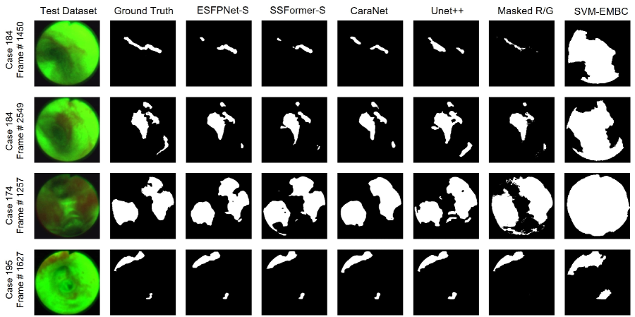
Figure 3: AFB Segmentation results. The first column is the original frame, and the second column gives the reference ground truth segmentation. Results for the other methods are ordered from best to worst.

Figure 4 next illustrates processing results for a 500-frame video clip from patient case 198, a new case that was not a part of our original train/validate/test AFB image dataset. The video clip illustrates a bronchoscopy exam as it starts in the main carina and then progresses to the right main bronchus and right upper lobe bronchus; it terminates at the lateral segmental bronchus inside the right middle lobe. As highlighted by red boxes in the figure, two lesions have been correctly found in the right middle lobe (duration $\approx$ 20 frames) and the lateral segmental bronchus (duration only a few frames). As the figure clearly shows, both SSFormer-S and ESFPNet-S successfully detect the lesions with high IoU value, with ESFPNet-S signaling fewer false positive frames.

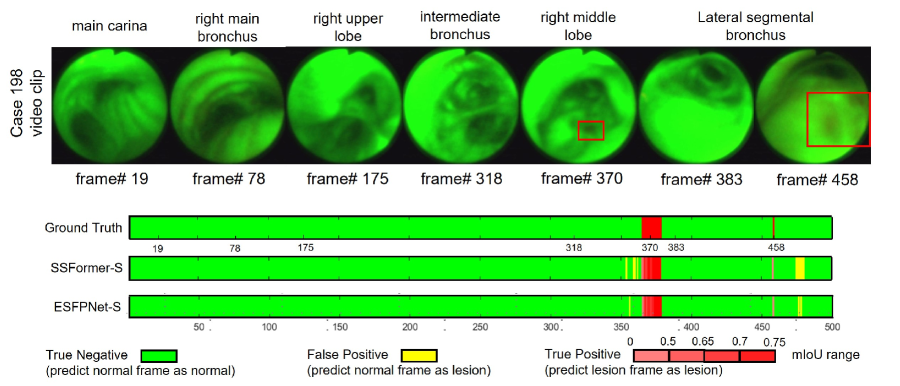
Figure 4: Test with a new 500-frame AFB bronchoscopy video clip using SSFormer-S and ESFPNet-S. Both SSFormer-S and ESFPNet-S successfully detect the lesions with high IoU values, while ESFPNet-S outputs fewer false positive frames.

As a final test, we implemented the ESFPNet-S into C++ on a Windows-10-based PC, which includes an Intel Xeon Gold 6230 CPU and NVIDIA RTX 3090 GPU. With this set up, we could then test the live real-time performance of the method for a complete end-to-end segmentation procedure. The complete procedure consisted of reading frames from the AFB video stream, image normalization and resizing, ESFPNet prediction analysis, and displaying the lesion segmentation results on the computer monitor. For a 1000-frame test, we achieved an average frame rate of 27 frames per second (FPS), essentially a real-time rate.

4.2 Tests on the polyp datasets

Tables 4-5 give experimental results for learning ability, generalizability, and power balance for the polyp datasets. These results clearly demonstrate the overall state-of-the-art capabilities of our proposed ESFPNet-L architecture for polyp segmentation. In particular, ESFPNet-L achieved the following:
1.) State-of-the-art (SOTA) learning ability on the CVC-ClinicDB benchmark dataset (Table 4).
2.) SOTA generalizability and power balance over the ETIS-LaribPolyDB benchmark data set (Tables 4-5).
Thus, we conclude that our architecture is very much a viable alternative for polyp segmentation, given its aoverall performance over these various benchmark datasets.

As final evidence, Figure 5 gives example polyp segmentation results, based on the models of Table 5. For the five polyp datasets, our ESFPNet-L shows its outstanding performance on both generalizability and learning ability.

Table 3: Quantitative comparison of learning ability

	CVC-ClinicDB		Kvasir
architectures	mDice	mIoU	mDice	mIoU
U-net++	0.915	0.865	0.863	0.818
Deeplabv3+	0.888	0.871	0.897	0.858
MSRF-Net	0.942	0.904	0.922	0.891
SSFormer-L	0.945	0.899	0.936	0.891
ESFPNet-L	0.949	0.907	0.931	0.887

Table 4: Generalizability test.

datasets	architectures	mDice	mIoU	$S_{\alpha}$	$E_{\phi}^{max}$	MAE
ETIS- LaribPolypDB	ESFPNet-T	0.781	0.701	0.866	0.910	0.016
	ESFPNet-S	0.807	0.730	0.879	0.916	0.015
	ESFPNet-L	0.827	0.752	0.892	0.935	0.011
CVC- ColonDB	ESFPNet-T	0.781	0.699	0.843	0.895	0.036
	ESFPNet-S	0.795	0.711	0.854	0.905	0.032
	ESFPNet-L	0.823	0.741	0.871	0.917	0.029

• BOLD values indicate the best results and underlined values indicate the second best results.

Table 5: Power balance experimental results.

architectures	Kvasir		CVC-ClinicDB		CVC-T		CVC-ColonDB		ETIS-LaribPolypDB
	mDice	mIoU	mDice	mIoU	mDice	mIoU	mDice	mIoU	mDice	mIoU
Unet++	0.818	0.746	0.823	0.750	0.710	0.627	0.512	0.444	0.398	0.335
SFA	0.723	0.611	0.700	0.607	0.297	0.217	0.469	0.347	0.467	0.329
CaraNet	0.918	0.865	0.936	0.887	0.903	0.838	0.773	0.689	0.747	0.672
SSFormer-L	0.917	0.864	0.906	0.855	0.895	0.827	0.802	0.721	0.796	0.720
ESFPNet-L	0.917	0.866	0.928	0.883	0.902	0.836	0.811	0.730	0.823	0.748

• BOLD values indicate the best results and underlined values indicate the second best results.

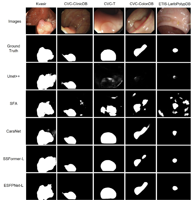
Figure 5: Polyp segmentation results.

5 DISCUSSION AND CONCLUSION

Bronchial lesions can be treated as biomarkers that signal lung cancer. These lesions, which can be detected by autofluorescence bronchoscopy, are useful for detecting lung cancer at the early stage. We have proposed ESFPNet for bronchial lesion segmentation and have applied it to a 20-patient AFB lung cancer patient dataset. Our results demonstrate superior segmentation performance over competing deep-learning architectures. Also, given the ESPFNet’s ability to produce results at essentially a real-time frame rate, it shows potential utility during live bronchoscopic airway exams. Finally, to the best of our knowledge, this is the first work for automatic real-time segmentation of bronchial lesions in AFB video.

As a second result, when ESFPNet was tested for colonic polyp segmentation over five standard publicly available datasets, it again showed excellent performance. These results therefore illustrates its general strong capability for medical image segmentation in other domains.

The proposed ESPFNet architecture incorporates a novel light-level feature pyramid decoder structure based on MiT encoders to efficiently and comprehensively use extracted image features. Through experiments with our AFB dataset, we showed that ESFPNet-S outperforms other famous models for the mDice and mIoU metrics. In addition, ESFPNet-S was shown to be a viable approach for real-time lesion segmentation and detection with AFB video clips. Finally, as demonstrated by the colonic polyp segmentation results, ESFPNet exhibits outstanding performance in terms of generalizability and learning ability over several large datasets.

Nevertheless, further improvements are possible to our work. First, using only 208 lesion frames to train our deep learning architecture is not realistically sufficient. Because of the high cost and difficulty in collecting further live human video data, we could use semi-supervised learning methods, such as contrastive learning, to train our model more rigorously. Second, far more extensive tests on AFB video clips, in addition to testing the method during a live procedure would give a more complete understanding of our architecture’s overall performance and viability for live clinical early lung cancer lesion detection. Third, we need to create more evidence that our feature pyramid is efficient and comprehensive in its use of the features extracted by the ESPFNet’s encoders; a possibility is to use attention heat maps to reflect the functionality of each decoding linear prediction layer.

- [1] Bray, F., Ferlay, J., Soerjomataram, I., Siegel, R. L., Torre, L. A., and Jemal, A., “Global cancer statistics 2018: Globocan estimates of incidence and mortality worldwide for 36 cancers in 185 countries,” CA: Cancer J. Clin. 68, 394–424 (Sept. 2018).
- [2] Inage, T., Nakajima, T., Yoshino, I., and Yasufuku, K., “Early lung cancer detection,” Clin. Chest Med. 39, 45–55 (2018).
- [3] Kusunoki, Y., Imamura, F., Uda, H., Mano, M., and Horai, T., “Early detection of lung cancer with laser-induced fluorescence endoscopy and spectrofluorometry,” Chest 118(6), 1776–1782 (2000).
- [4] Finkšt, T., Tasič, J. F., Zorman-Terčelj, M., and Zajc, M., “Autofluorescence bronchoscopy image processing in the selected colour spaces,” STROJ VESTN-J MECH E (SVJME) 58(9), 501–508 (2012).
- [5] Finkšt, T., Tasič, J. F., et al., “Classification of malignancy in suspicious lesions using autofluorescence bronchoscopy,” Strojnivski J. Mech. Eng. 63(12), 685–695 (2017).
- [6] Chang, Q., Bascom, R., Toth, J., Ahmad, D., and Higgins, W. E., “Autofluorescence bronchoscopy video analysis for lesion frame detection,” in [42nd Annu. Int. Conf. IEEE Eng. Med. Biol. - Proc. (EMBC) ], 1556–1559, IEEE (2020).
- [7] Zhou, Z., Siddiquee, M. M. R., Tajbakhsh, N., and Liang, J., “Unet++: A nested u-net architecture for medical image segmentation,” in [Deep learning in medical image analysis and multimodal learning for clinical decision support ], 11045, 3–11, Springer (Sept. 2018).
- [8] Ronneberger, O., Fischer, P., and Brox, T., “U-net: Convolutional networks for biomedical image segmentation,” in [Int. Conf. Med. Image Comp. Computer-assisted Interv. (MICCAI) ], 234–241 (2015).
- [9] Lou, A., Guan, S., and Loew, M., “Caranet: Context axial reverse attention network for segmentation of small medical objects,” arXiv preprint arXiv:2108.07368 (2021).
- [10] Xie, E., Wang, W., Yu, Z., Anandkumar, A., Alvarez, J. M., and Luo, P., “Segformer: Simple and efficient design for semantic segmentation with transformers,” in [Adv Neural Inf Process Syst. (NeurIPS) ], Ranzato, M., Beygelzimer, A., Dauphin, Y., Liang, P., and Vaughan, J. W., eds., 34, 12077–12090, Curran Associates, Inc. (27 Oct. 2021).
- [11] Wang, J., Huang, Q., Tang, F., Meng, J., Su, J., and Song, S., “Stepwise feature fusion: Local guides global,” arXiv preprint arXiv:2203.03635 (2022).
- [12] Badrinarayanan, V., Kendall, A., and Cipolla, R., “Segnet: A deep convolutional encoder-decoder architecture for image segmentation,” IEEE Trans. Pattern Anal. Mach. Intell. (TPAMI) 39, 2481–2495 (Jan. 2017).
- [13] Yuan, L., Chen, Y., Wang, T., Yu, W., Shi, Y., Jiang, Z.-H., Tay, F. E., Feng, J., and Yan, S., “Tokens-to-token vit: Training vision transformers from scratch on imagenet,” in [Proc. IEEE Comput. Soc. Conf. Comput. Vis. (ICCV) ], 558–567 (Oct. 2021).
- [14] Deng, J., Dong, W., Socher, R., Li, L.-J., Li, K., and Fei-Fei, L., “Imagenet: A large-scale hierarchical image database,” in [2009 IEEE Conf. Computer Vision Patt. Recog. (CVPR) ], 248–255, IEEE (2009).
- [15] Raghu, M., Unterthiner, T., Kornblith, S., Zhang, C., and Dosovitskiy, A., “Do vision transformers see like convolutional neural networks?,” in [Adv Neural Inf Process Syst. (NeurIPS) ], Ranzato, M., Beygelzimer, A., Dauphin, Y., Liang, P., and Vaughan, J. W., eds., 34, 12116–12128, Curran Associates, Inc. (27 Oct. 2021).
- [16] Lou, A. and Loew, M., “Cfpnet: Channel-wise feature pyramid for real-time semantic segmentation,” arXiv preprint arXiv:2103.12212 (2021).
- [17] Jha, D., Smedsrud, P. H., Riegler, M. A., Halvorsen, P., Lange, T. d., Johansen, D., and Johansen, H. D., “Kvasir-seg: A segmented polyp dataset,” in [International Conference on Multimedia Modeling (MMM) ], 11962, 451–462, Springer (Dec. 2019).
- [18] Bernal, J., Sánchez, F. J., Fernández-Esparrach, G., Gil, D., Rodríguez, C., and Vilariño, F., “Wm-dova maps for accurate polyp highlighting in colonoscopy: Validation vs. saliency maps from physicians,” Comput. Med. Imaging Graph (CMIG) 43, 99–111 (July 2015).
- [19] Vázquez, D., Bernal, J., Sánchez, F. J., Fernández-Esparrach, G., López, A. M., Romero, A., Drozdzal, M., and Courville, A., “A benchmark for endoluminal scene segmentation of colonoscopy images,” J. Healthc. Eng (JHE) 2017 (Jul. 2017).
- [20] Tajbakhsh, N., Gurudu, S. R., and Liang, J., “Automated polyp detection in colonoscopy videos using shape and context information,” IEEE Trans. Med. Imaging. (TMI) 35, 630–644 (Oct. 2015).
- [21] Silva, J., Histace, A., Romain, O., Dray, X., and Granado, B., “Toward embedded detection of polyps in wce images for early diagnosis of colorectal cancer,” Int. J. Comput. Assist. Radiol. Surg. (IJCARS) 9, 283–293 (March 2014).
- [22] Chen, L.-C., Zhu, Y., Papandreou, G., Schroff, F., and Adam, H., “Encoder-decoder with atrous separable convolution for semantic image segmentation,” in [Proc. Euro. Conf. Comput. Vis. (ECCV) ], 801–818 (Sept. 2018).
- [23] Fang, Y., Chen, C., Yuan, Y., and Tong, K.-y., “Selective feature aggregation network with area-boundary constraints for polyp segmentation,” in [Med Image Comput Comput Assist Interv (MICCAI) ], 11764, 302–310, Springer International Publishing (10 Oct. 2019).
- [24] Srivastava, A., Jha, D., Chanda, S., Pal, U., Johansen, H. D., Johansen, D., Riegler, M. A., Ali, S., and Halvorsen, P., “Msrf-net: A multi-scale residual fusion network for biomedical image segmentation,” IEEE J. Biomed. Health Inform. (JBHI) 26, 2252–2263 (May 2022).
- [25] Fan, D.-P., Ji, G.-P., Zhou, T., Chen, G., Fu, H., Shen, J., and Shao, L., “Pranet: Parallel reverse attention network for polyp segmentation,” in [Med Image Comput Comput Assist Interv (MICCAI) ], 12266, 263–273, Springer International Publishing (Sept. 2020).
- [26] Fan, D.-P., Cheng, M.-M., Liu, Y., Li, T., and Borji, A., “Structure-measure: A new way to evaluate foreground maps,” in [Proc. IEEE Comput. Soc. Conf. Comput. Vis. (ICCV) ], 4548–4557 (Oct. 2017).
- [27] Fan, D.-P., Gong, C., Cao, Y., Ren, B., Cheng, M.-M., and Borji, A., “Enhanced-alignment measure for binary foreground map evaluation,” arXiv preprint arXiv:1805.10421 (2018).