Hard-disk computer simulations—a historic perspective

Abstract

We discuss historic pressure computations for the hard-disk model performed since 1953, and compare them to results that we obtain with a powerful event-chain Monte Carlo and a massively parallel Metropolis algorithm. Like other simple models in the sciences, such as the Drosophila model of biology, the hard-disk model has needed monumental effort to be understood. In particular, we argue that the difficulty of estimating the pressure has not been fully realized in the decades-long controversy over the hard-disk phase-transition scenario. We present the physics of the hard-disk model, the definition of the pressure and its unbiased estimators, several of which are new. We further treat different sampling algorithms and crucial criteria for bounding mixing times in the absence of analytical predictions. Our definite results for the pressure, for up to one million disks, may serve as benchmarks for future sampling algorithms. A synopsis of hard-disk pressure data as well as different versions of the sampling algorithms and pressure estimators are made available in an open-source repository.

I Introduction

In fundamental physics, the most detailed descriptions of physical reality are not always the best. In our quantum-mechanical world, many phenomena are indeed described classically, without the elaborate machinery of wavefunctions and density matrices. The exact thermodynamic singularities of helium, a quantum liquid, at the famous lambda transition [1] are for example obtained by a seemingly unrelated model of classical two-component spins [2, 3, 4, 5] on a three-dimensional lattice rather than by some quantum-mechanical representation of all atoms in the continuum [6]. Renormalization-group theory [7] guarantees that the simple classical spin model exactly describes experiments in the quantum liquid [8, 9]. The universality of simple models is also found in other sciences. In biology, the study of the fruit fly Drosophila has gradually evolved from a subject of entomology, the science of insects, to a parable for higher animals, where it allows one to appreciate gene damage [10] from radiation. In recent decades, it was moreover understood that many of the genes of the Drosophila have exactly the same function as genes in vertebrates, including humans. In physics as in biology, “(t)his remarkable conservation came as a big surprise. It had been neither predicted nor expected” [11], to cite a Nobel-prize winner.

Paradoxically, even simple models in science, those stripped to their bare bones, can take monumental effort and decades of research to be understood fully. This is the case for the Drosophila fly that entered research laboratories around 1905 [12], and then gradually turned into a model organism [13]. It is also what happened to the simplest of all particle models, the hard-disk model, which is the focus of the present work. The model consists of $N$ identical classical disks with positions inside a box and with velocities. Disks fly in straight-line trajectories, except when they collide with each other or with an enclosing wall. The elementary collision rules are borrowed from billiards. The hard-disk model caricatures two-dimensional fluids: It lacks the explicit interparticle attractions of more realistic descriptions, yet it shows almost all the interesting properties of general particle systems. Moreover, its observed phase behavior [14] was understood in terms of topological phase transitions, just like classical continuous spin models in two dimensions [15]. The interpretation common to both cases was unsuspected from the conventional Landau theory of phase transitions.

Only few characteristics of the hard-disk model are known from rigorous mathematics. The first was proven by Daniel Bernoulli in 1738 [16], namely that the temperature, which is linked to the mean-square velocity of the disks, plays no role in their spatial distribution. It was also proven [17, 18] that the hard-disk model, as a dynamical system with positions and velocities evolving under Newton’s laws, can be described statistically with positions that all have equal statistical weight. It is furthermore shown rigorously that, at small finite density, the model is fluid [19, 20], justifying analytic expansions developed in the $19$th century [21] to link dilute hard disks to the ideal gas of non-interacting particles. For high densities, it was established that at close packing, the hard-disk model forms a hexagonal crystal [22]. However, for all densities below close packing, this crystalline structure is destroyed [23, 24] by long-wavelength fluctuations. The invention of simulation methods, and their application to this very model of hard disks ever since the 1950s, was meant to overcome the scarcity of analytical results.

With its stripped-down interactions, the hard-disk model is indeed simple. In particular, the model lacks attractive forces that would pull the disks together. It is for this reason that, for a long time, hard disks and hard spheres (in three dimensions) were considered too simple to show a phase transition from an disordered fluid to a solid [25, 26]. In two dimensions, furthermore, ordered phases were expected not to exist for theoretical reasons that were considered sufficiently solid to formally exclude any transition [27]. Initial computer simulations, in 1953, in the same publication that introduced the Metropolis algorithm [28], accordingly found that “(t)here is no indication of a phase transition”. It thus came as an enormous surprise when, in 1962, Alder and Wainwright [14] identified a loop in the equation of state (see Fig. 1), suggesting [29] a phase transition between a fluid at low density and a solid (that was not supposed, at the time, to exist) at high density. This laid the ground work for the Kosterlitz–Thouless–Halperin–Nelson–Young theory of melting in two-dimensional particle systems [30, 31, 32]. Even after this important conceptual advance, the phase behavior of the hard-disk model remained controversial for another fifty years, until an analysis [33] based on the powerful event-chain Monte Carlo (ECMC) algorithm [34] showed that hard disks melt through a first-order fluid–hexatic phase transition combined with a Kosterlitz–Thouless transition between the hexatic and the solid, thus proposing a new scenario.

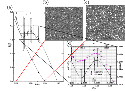
Figure 1: Hard disks in a periodic box. (a): Equation of state (pressure vs. volume) computed in 1962 by Alder and Wainwright [14] (b) and (c): Samples of $870$ disks at densities $\eta=0.726$ and $\eta=0.672$. (d): Pressures for $N=870$ from (a) compared with ECMC results (this work) for aspect ratio $\alpha\!=\!(9\!:\!8\sqrt{3}/2)$ (cf Fig. 10 for an analysis of convergence behavior).

In this work, we discuss the hard-disk model in a computational and historical context, concentrating on the pressure as a function of the volume. The reason for this restriction of scope on pressures rather than on phases is that the aforementioned fifty-year controversy was rooted in difficulties in computing the pressure. After a short introduction to the physics of the hard-disk model, we review the thermodynamic and kinematic pressure definitions, and show that they are perfectly equivalent even for finite systems. Nevertheless, the pressure may be anisotropic and depend on the shape of the system, rather than being only a function of system volume. We discuss pressure estimators, with a focus on those that are unbiased at finite $N$ and convenient to use. We furthermore clarify that different sampling algorithms (molecular dynamics, reversible and non-reversible MCMC) all rigorously sample the same equal-weight Boltzmann distribution of positions although the time scales for convergence can differ widely even for local algorithms, and can reach years and even decades of computer time for moderate system sizes. This was not understood in many important historical contributions. With all this material in hand, we confront past results with massive computations performed for this work, thus providing definite high-precision pressure estimates for the hard-disk model that may serve as benchmarks for the future. With its rich phenomenology and its intractable mathematics, this simple model has become the Drosophila for particle systems and for two-dimensional phase transitions. It has served as a parable for difficult computing problems and as a platform for development of MCMC and of molecular dynamics. This fascinating model has yet to be fully understood. We aim at providing a solid base for future work.

The plan of this work is as follows. In Section II, we discuss the fundamentals of the hard-disk model, from the definitions of densities and volumes to an overview of its physical properties. In Section III, we discuss sampling algorithms (molecular dynamics and Markov-chain Monte Carlo (MCMC)) and pressure estimators for this model, concentrating on new developments. In Section IV, we digitize, discuss, and make available numerical computations of the equation of state performed since the paper by Metropolis et al., in 1953, and superpose them with large-scale computations done for this work. Section V contains our conclusions. We also provide information on statistical analysis (Appendix A) and introduce to the HistoricDisks open-source software package, which collects pressure data since 1953, and implements sampling algorithms and pressure estimators (Appendix B) that were used in this work.

II Hard-disk model

The hard-disk model consists of $N$ impenetrable, identical, classical disks of radius $\sigma$ and mass $m$, that are perfectly elastic. Collisions are instantaneous; they cause no deformations and induce no rotations. Pair collisions conserve momentum and energy. Disks evolve in a fixed rectangular box of sides $L_{x}$ and $L_{y}$ (specified through the aspect ratio $\alpha\!=\!(L_{x}\!:\!L_{y})$), which may have periodic boundary conditions (“periodic” box), or else hard-wall boundary conditions (“non-periodic” box). The two-dimensional volume (area) is $V=L_{x}\times L_{y}$. In the $NVT$ ensemble that we consider here, $N$, $L_{x}$, and $L_{y}$ are fixed. For the hard-disk system, the microcanonical ensemble (of constant energy $E$) and the canonical ensemble (of constant temperature $T$) are almost equivalent, and we connect the two throughout this work. In other ensembles, the box can be of varying dimensions [35, 36, 37], and $N$ might vary [38]. The disk $i$ is described by the position of its center $\mathbf{x}_{i}=(x_{i},y_{i})$, and possibly by a velocity $\mathbf{v}_{i}=(v_{x,i},v_{y,i})$. We denote the set of positions and velocities by $\mathbf{x}=\{\mathbf{x}_{1},\ldots,\mathbf{x}_{N}\}$ and $\mathbf{v}=\{\mathbf{v}_{1},\ldots,\mathbf{v}_{N}\}$, respectively.

II.1 Basic definitions and properties

We now discuss additional characteristics of the hard-disk model and define its Newtonian dynamics. Furthermore, we summarize the physics of two-dimensional particle systems.

II.1.1 System definitions, basic properties

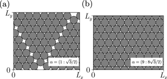
Figure 2: Packings for $N=72$ disks for different aspect ratios $\alpha$. (a): Periodic box with $\alpha=(1:\sqrt{3}/2)$, with conjectured optimal packing. (b): Periodic box with $\alpha=(9:8\sqrt{3}/2)$ at the close-packing density $\eta=\pi/(2\sqrt{3})$.

In the limit $N\to\infty$, the properties of a particle system with short-range interactions are independent of the boundary conditions. At finite $N$, in contrast, the bulk part of the free energy (that scales as $V$) cannot be separated from the surface term (that, in two dimensions, scales as $\sqrt{V}$). For example, a close-packed crystal of $N=72=8\times 9$ disks can fit into a periodic box of aspect ratio $\alpha\!=\!(9\!:\!8\sqrt{3}/2)$, whereas the maximum density for the same $N$ in a box with $\alpha\!=\!(1\!:\!\sqrt{3}/2)$ is slightly smaller (see Fig. 2). Evidently, the pressure in a box containing a finite number of disks depends on its aspect ratio.

The following conventions for the volume or its inverse, the density, have been commonly used in the literature. The first is the volume $V=L_{x}\times L_{y}$ normalized by that of a perfect hexagonal packing $V_{0}=N(2\sigma)^{2}\sqrt{3}/2$ (as in Fig. 2b). Second is the covering density $\eta$, the total volume of all disks normalized by the box volume $V$. Third is the reduced density $\rho$, the number $N$ of disks of radius $\frac{1}{2}$ divided by the volume and, finally, the inverse normalized density $\nu/(2\sigma)^{2}$ with $\nu=1/\rho$. These quantities are related as follows:

$$\frac{V}{V_{0}} =\frac{\pi}{2\sqrt{3}}\frac{1}{\eta}=\frac{2}{\sqrt{3}}\frac{\nu}{(2\sigma)^{2}}\geq 1,$$ (1)

$$\ \eta =\frac{\pi}{2\sqrt{3}}\frac{V_{0}}{V}=\frac{N}{V}\pi\sigma^{2}\leq 0.907,$$

$$\rho =\eta\frac{4}{\pi}=\frac{V_{0}}{V}\frac{2}{\sqrt{3}}=\frac{(2\sigma)^{2}}{\nu}\leq 1.155,$$

$$\frac{\nu}{(2\sigma)^{2}} =\frac{\sqrt{3}}{2}\frac{V}{V_{0}}=\frac{\pi}{4}\frac{1}{\eta}=\frac{1}{\rho}\geq 0.866.$$

We will re-plot published equations of state with all four units, thus simplifying the comparison of data.

In the hard-disk model, all configurations have zero potential energy, and the Newtonian time evolution conserves the kinetic energy. Pairs of disks collide such that, in their center-of-mass coordinate system, they rebound from their line of contact with conserved parallel and reversed perpendicular velocities [39]. At a wall collision, the velocity component of a disk parallel to the wall remains the same while the perpendicular velocity $v^{\perp}_{\text{wall}}$ is reversed. When, at the initial time $t=0$, all velocities are rescaled by a factor $\gamma$, the entire trajectory transforms as

$$\{\mathbf{x}_{1}(t),\ldots,\mathbf{x}_{N}(t)\}\xrightarrow{\mathbf{v}_{i}\to\gamma\mathbf{v}_{i}\forall i}\{\mathbf{x}_{1}(\tfrac{t}{\gamma}),\ldots,\mathbf{x}_{N}(\tfrac{t}{\gamma})\}.$$ (2)

This property of hard-sphere models was already noticed by Daniel Bernoulli [16].

Statistically, during the Newtonian hard-disk time evolution, the sets of positions and of velocities are mutually independent. All positions $\mathbf{x}$ that correspond to $N$-disk configurations have the same statistical weight $\pi$ with a Cartesian density measure and, in a non-periodic box, the velocities are randomly distributed on the surface of the hypersphere in $2N$-dimensional space with radius $R_{v}=\sqrt{2E/m}$, where $E$ is the conserved (microcanonical) energy. The measure in the $4N$-dimensional sample space of positions and velocities is thus

$$\mathrm{d}\pi\propto\Theta(\mathbf{x})\mathrm{d}^{N}\mathbf{x}\;\mathrm{d}^{N}\mathbf{v}\,\delta\left(E-\sum_{i}m\mathbf{v}_{i}^{2}/2\right),$$ (3)

where $\Theta(\mathbf{x})=1$ for positions that correspond to hard-disk configurations and $\Theta(\mathbf{x})=0$ otherwise. In a periodic box, in addition, the two components of the total velocity and the position of the center of mass in the rest frame are conserved. For large $N$, where the ensembles are equivalent, the microcanonical energy per disk corresponds to $E/N=k_{\text{B}}T=1/\beta$, where $k_{\text{B}}$ is the Boltzmann constant and $T$ the temperature of the canonical ensemble. The spatial part of the measure of Eq. (3) remains unchanged, and the uniform velocity distribution on the surface of the hypersphere in $2N$ dimensions implies that the one-particle, marginal distribution of velocity components becomes Gaussian:

$$\pi(v_{i,x})\propto\exp\left(-\beta mv_{i,x}^{2}/2\right)\quad(N\to\infty)$$ (4)

(and analogously for $v_{i,y}$, see [39, Sect. 2.1.1]).

The probability distribution of the velocity perpendicular to a wall $v^{\perp}_{\text{wall}}$ (essentially the histogram of momentum transfers with the walls at the discrete wall-collision times) differs from Eq. (3). For $N\to\infty$, this distribution is biased by a factor $|v^{\perp}_{\text{wall}}|$ with respect to the Maxwell distribution:

$$\pi(|v^{\perp}_{\text{wall}}|)\propto|v^{\perp}_{\text{wall}}|\exp\left(-\beta m(v^{\perp}_{\text{wall}})^{2}/2\right),$$ (5)

which has been described through the “Maxwell boundary condition” (see [39, Sect. 2.3.1]). For finite $N$, the same biasing factor appears. The distribution of the velocity perpendicular to a wall is derived from the surface element on the hypersphere of radius $R_{v}=\sqrt{v_{1}^{2}+\dots+v_{n}^{2}}$ in $n=2N$ dimensions:

$$\mathrm{d}\Omega=R_{v}^{n-1}\sin^{n-2}\!\,\phi_{1}\sin^{n-3}\!\,\phi_{2}\dots\sin\!\,\phi_{n-2}\mathrm{d}\phi_{1}\dots\mathrm{d}\phi_{n-1},$$ (6)

where $\phi_{1},\ldots,\phi_{n-2}\in[0,\pi]$ and $\phi_{n-1}\in[0,2\pi]$, and where only $v_{1}=R_{v}\cos\!\,\phi_{1}$ is expressed in terms of a single angle. It is thus convenient to identify $v_{1}$ with $v^{\perp}_{\text{wall}}$. The radius $R_{v}$ of the hypersphere at the microcanonical energy $E=mR_{v}^{2}/2$ is related to the inverse temperature in the canonical ensemble as $R_{v}^{2}=2N/(m\beta)$. With the integrals

$$A =\int_{0}^{\pi}\mathrm{d}\phi_{1}|\cos\!\,\phi_{1}|\sin^{n-2}\!\,\phi_{1}=\frac{2}{n-1},$$ (7)

$$B =\int_{0}^{\pi}\mathrm{d}\phi_{1}\sin^{n-2}\!\,\phi_{1}=\sqrt{\pi}\frac{\Gamma[(n-1)/2]}{\Gamma(n/2)},$$

this yields:

$$\left\langle\frac{1}{|v^{\perp}_{\text{wall}}|}\right\rangle =\frac{1}{R_{v}}\frac{B}{A}=\frac{\sqrt{\pi}}{R_{v}}\frac{\Gamma(N+\frac{1}{2})}{\Gamma(N)}\stackrel{{\scriptstyle N\to\infty}}{{\longrightarrow}}\sqrt{\frac{\pi m\beta}{2}},$$ (8a)

$$\left\langle|v^{\perp}_{\text{wall}}|\right\rangle =R_{v}\frac{B}{2NA}=\frac{R_{v}\sqrt{\pi}}{2N}\frac{\Gamma(N+\frac{1}{2})}{\Gamma(N)}\stackrel{{\scriptstyle N\to\infty}}{{\longrightarrow}}\sqrt{\frac{\pi}{2m\beta}},$$ (8b)

where in the limit $N\to\infty$ the ratio of the $\Gamma$ functions approaches $\sqrt{N}$. The relative perpendicular velocities $\Delta v^{\perp}_{ij}$ (the projection of the relative velocity $\mathbf{v}_{i}-\mathbf{v}_{j}$ perpendicular to the interface separating disks $i$ and $j$ at their collision) is, similarly:

$$\left\langle\frac{1}{|\Delta v^{\perp}_{ij}|}\right\rangle =\frac{\sqrt{2\pi}}{R_{v}}\frac{\Gamma(N+\frac{1}{2})}{\Gamma(N)}\stackrel{{\scriptstyle N\to\infty}}{{\longrightarrow}}\sqrt{\pi m\beta},$$ (9a)

$$\left\langle|\Delta v^{\perp}_{ij}|\right\rangle =\frac{R_{v}\sqrt{\pi}}{\sqrt{2}N}\frac{\Gamma(N+\frac{1}{2})}{\Gamma(N)}\stackrel{{\scriptstyle N\to\infty}}{{\longrightarrow}}\sqrt{\frac{\pi}{m\beta}}.$$ (9b)

II.1.2 Pair correlations, entropic phase transition

In the hard-disk model, the Boltzmann weights are the same for all sets of disk positions, since there are no explicitly varying interactions. In consequence, the two possible fluid phases (namely the gas and the liquid) are confounded. A purely entropic “depletion” interaction [40] between disks nevertheless arises from the presence of other disks, effectively driving phase transitions. The three phases of the hard-disk model are fluid (with exponential decays of the orientational and positional correlation functions), hexatic (with an algebraic decay of orientational and exponential decay of positional correlations), and solid (with long-range orientational correlations and an algebraic decay of positional correlations). The hexatic and solid phases have only been identified through numerical simulations, and mathematical proofs of their existence are still lacking.

II.2 Hard-disk thermodynamics

In statistical mechanics, a homogeneous system (composed of, say, $N$ particles in a fixed box) is described by an equation of state connecting two quantities, as for example the volume and the pressure. When for some volumes, a homogeneous phase may not exist, two (or exceptionally three) phases may coexist. We now link the definitions of the pressure from the thermodynamic and kinematic viewpoints and then discuss phase coexistence in finite systems.

II.2.1 Pressure, thermodynamic and kinematic definitions

In statistical mechanics, the pressure $P$ is given by the change of the free energy with the system volume:

$$\beta P=\frac{\partial\log\!\,Z}{\partial V}\stackrel{{\scriptstyle V^{\prime}\to V}}{{=}}\frac{1}{V-V^{\prime}}\frac{Z-Z^{\prime}}{Z}.$$ (10)

with $Z$ the partition function and $Z^{\prime}\equiv Z(V^{\prime})$. For hard disks and related models, the rightmost fraction in Eq. (10) expresses the probability that a sample in the original box of volume $V$ is eliminated in the box of reduced volume $V^{\prime}<V$. In rift-pressure estimators [41], the volume $V$ of an $L_{x}\times L_{y}$ box is reduced by removing an infinitesimal vertical or horizontal slab (a “rift”), yielding the components $P_{x}$ and $P_{y}$ of the pressure. Rifts can be placed anywhere in the box, and one may even average any given hard-disk sample over all vertical or horizontal rift positions (see Subsection III.3). We will also discuss homothetic pressure estimators, where all box dimensions and disk coordinates are scaled down by a common factor. Used for decades, they estimate the pressure $P=(P_{x}+P_{y})/2$.

Besides the thermodynamic definition of the pressure, one can also define the kinematic pressure as the exchange of momentum with the enclosing walls. However, thermodynamic and kinematic pressures are rigorously identical already at finite $N$, and the corresponding estimators can be transformed into each another. This is also true for the pressure estimators built on the virial formalism that we also discuss.

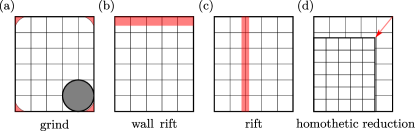
Figure 3: Volume reductions for a non-periodic box. (a): Pathological corner-grind volume reduction, that eliminates no samples for sufficiently large $\sigma$. (b): Horizontal wall rift used to estimate the pressure $P_{y}$. (c): Vertical rift used to estimate $P_{x}$. (d): Homothetic volume reduction.

II.2.2 Equation of state, phase coexistence

In the thermodynamic limit, the stability of matter is expressed through a positive compressibility $\kappa=-(\partial V/\partial P)/V$. For a finite system in the $NVT$ ensemble, this is not generally true in a presence of a first-order phase transition, where two coexisting phases are separated by an interface with its own interface free energy.

In a periodic two-dimensional box for finite $N$, on increasing the density (decreasing the volume), a first-order phase transition first creates a bubble of the denser phase in the less dense phase (for hard disks: a hexatic bubble inside the fluid). The stabilization of this bubble requires an extra “Laplace” pressure corresponding to the surface tension, which renders the overall pressure non-monotonic with $V$ [29]. At larger densities, the bubble of the minority phase transforms into a stripe that winds around the periodic box. In the stripe regime, the length of the two interfaces and thus the interface free energy do not change with $V$, so that the pressure remains approximately constant. Finally, one obtains a bubble of the less dense phase (the fluid) in the surrounding denser (hexatic) phase (see Fig. 4). The phase coexistence is specific to the $NVT$ ensemble as certain specific volumes $V/V_{0}$ do not correspond to densities $\eta=(N/V)\pi\sigma^{2}$ of a homogeneous stable phase for $N\to\infty$. Phase coexistence is absent in the $NPT$ ensemble. The pressure is then the control variable, and the volume $V/V_{0}$ is discontinuous at the transition, providing for a simpler physical picture. However, in the $NPT$ ensemble and its variants, sampling algorithms generally converge even more slowly than in the $NVT$ ensemble.

The phase coexistence and the non-monotonous equation of state are genuine equilibrium features at finite $N$. Moreover, the spatially inhomogeneous phase-separated equilibrium state is reached from homogeneous initial configurations through a slow coarsening process, whose dynamics depends on the sampling algorithm.

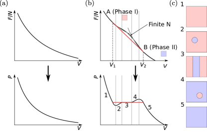
Figure 4: First-order phase transition in the $NVT$ ensemble. (a): Free energy with increasing second derivative, and thus a monotonously decreasing pressure. (b): Free energy with—for the infinite system—metastable branches starting at volumes $V_{1}$ and $V_{2}$, and a non-monotonous equilibrium pressure $P$ for finite $N$. (c): Sequence of five regimes in a finite two-dimensional periodic box, with pure (1,5), bubble (2,4) and stripe (3) phases.

III Sampling algorithms and pressure estimators

In the present section, we discuss sampling algorithms (molecular dynamics, MCMC) and pressure estimators for the hard-disk model. All algorithms are unbiased and correct to machine precision. For example, molecular dynamics implements the Newtonian time evolution of disks without discretizing time. The reversible Monte Carlo algorithms, from the historic Metropolis algorithm to the recent massively parallel Monte Carlo (MPMC) on graphics-card computers, satisfy the detailed-balance condition: the net equilibrium flow vanishes between any two samples. The non-reversible ECMC algorithms only satisfy the global-balance condition, and samples live in an extended “lifted” sample space.

Besides the sampling algorithms, we also discuss pressure estimators, including recent ones that overcome the limitations of the traditional approaches. Thermodynamic pressure estimators compute the probability with which a sample is eliminated as the box is reduced in size while kinematic pressure estimators determine the momentum fluxes at the walls or inside the box. Importantly, both types of estimators have the same expectation value (the pressure $P$ or its components $P_{x}$ or $P_{y}$), and they merely differ in their efficiency and ease of use. Even at finite $N$, there is thus no ambiguity in the definition of the pressure. The various estimators play a key role in the equation-of-state computations in Section IV. All algorithms and estimators are cross-validated for four disks in a non-periodic square box (see Appendix B.2.1). These tiny simulations illustrate the absence of any finite-$N$ bias in the pressure estimators.

III.1 Event-driven molecular dynamics (EDMD)

Event-driven molecular dynamics (EDMD) [42] implements the Newtonian time evolution for the hard-disk model by stepping forward from one event (pair collision or wall collision) to the next. Between collisions, the disks move with constant velocities. Collisions of more than two disks, or simultaneous collisions can be neglected. For large run times $\tau_{\text{sim}}$, if the sample space is connected, molecular dynamics samples the equilibrium distribution of positions and velocities of Eq. (3).

III.1.1 Naive molecular-dynamics program

From a given set of positions and velocities for $N=4$ disks in a non-periodic box, our naive EDMD code computes the minimum over all pair collision times for the $N(N-1)/2$ pairs of disks, and over the wall collision times for the $N$ disks. This minimum corresponds to a unique collision event (multiple overlaps appearing with finite-precision arithmetic can be treated in an ad-hoc fashion). The code then updates all the positions and the velocities of the colliding disks. This algorithm is of complexity $\mathcal{O}\left(N^{2}\right)$ per event. A related naive program in a periodic box (with arbitrary $N$) is used for cross-validation of other algorithms. Practical implementations of EDMD process the collisions through floating-point arithmetic. As the hard-disk dynamics is chaotic for almost all initial configurations, trajectories for different precision levels quickly diverge and only the statistical properties of the trajectories are believed to be correct.

III.1.2 Modern hard-disk molecular dynamics

The complexity of EDMD can be reduced from the naive $\mathcal{O}\left(N^{2}\right)$ per event scaling to $\mathcal{O}\left(\log N\right)$. This is because the collisions of a given disk must only be tracked with other disks in a local neighborhood (reducing by itself the complexity to $\mathcal{O}\left(N\right)$) and because the collision of two disks $i$ and $j$ only modifies the future collision times for pairs involving $i$ or $j$ (see [43, 44]). This algorithm keeps $\mathcal{O}\left(N\right)$ candidate events of which a finite number must be updated after each event. Using a heap data structure, this is of complexity $\mathcal{O}\left(\log\!\,N\right)$, while the retrieval of the shortest candidate event time (the next event time) is $\mathcal{O}\left(1\right)$. Although the update of the event times involves elaborate book-keeping, and although the processing of events according to collision rules is time-consuming, the EDMD algorithm is thus fairly efficient. It has been successfully used for the hard-disk model up to intermediate sizes ($N\lesssim 256^{2}$ in the transition region). Open-source implementations of this algorithm are available [45]. The EDMD algorithm has not been successfully parallelized, despite some efforts in that direction [46].

III.2 Hard-disk Markov-chain Monte Carlo

Hard-disk Monte-Carlo algorithms consider a sample space consisting of the $N$ positions. Initial samples that are easy to construct, are modified through reversible or non-reversible schemes. In the large-time limit, the equal-probability measure of the positions in Eq. (3) is reached.

III.2.1 Local hard-disk Metropolis algorithm

In the local hard-disk Metropolis algorithm [28], at each time step, a small random displacement of a randomly chosen disk is accepted if the resulting sample is legal and is rejected otherwise. A move and its inverse are proposed with the same probability, so that the algorithm satisfies the detailed-balance condition with a constant equilibrium probability, and the net probability flows vanish.

The local Metropolis algorithm has been much used to obtain the hard-disk equation of state. On a modern single-core central-processing unit (CPU), this algorithm realizes roughly $\sim 10^{10}$ moves per hour. (For simplicity, we use “moves” for “proposed moves”.) However, its convergence is very slow. In Section IV.2.2, we will show evidence of mixing times [47] in excess of 10 years of CPU time for $\sim 10^{6}$ disks. The sequential variant of the local Metropolis algorithm updates the disk $i+1$ (identifying $N+1\equiv 1$) at time $t+1$ after having updated disk $i$ at time $t$. This non-reversible version runs slightly faster as it requires fewer random numbers per move, but the performance gain is minimal.

III.2.2 Massively parallel Monte Carlo (MPMC) algorithm

The MPMC algorithm generalizes the local Metropolis algorithm for implementation on graphical processing units (GPU) [48]. It uses a four-color checkerboard of rectangular cells of sides larger than $2\sigma$, that is superposed onto the periodic box and is compatible with the periodic boundary conditions. Cells of the same color are distant by more than $2\sigma$. They are aligned with the $\hat{\mathbf{e}}_{x}$ and $\hat{\mathbf{e}}_{y}$ axes. The MPMC algorithm samples one of the four colors, and then independently updates disks in all corresponding cells using the local Metropolis algorithm with the additional constraint that disks cannot leave their cells (see Fig. 5). After a certain time, the color is resampled. The checkerboard is frequently detached from the box, then randomly translated and repositioned, rendering the algorithm irreducible.

On a single NVIDIA GeForce RTX3090 GPU, our MPMC code reaches $2.1\times 10^{13}$ moves per hour, an order of magnitude more than an earlier implementation [49, Table II]. Repositioning the checkerboard is computationally cheap and is done often enough for the convergence time, measured in moves, to be only slightly larger than for the local Metropolis algorithm.

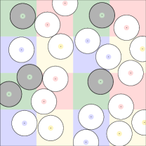
Figure 5: Four-color checkerboard decomposition in a periodic box, with cells larger than $2\sigma$. If the green color is chosen, highlighted disks may move, but cannot leave their cells. Disks in different green cells do not communicate.

III.2.3 Hard-disk event-chain Monte Carlo (ECMC)

Hard-disk ECMC is a non-reversible continuous-time “lifted” Markov chain [34] in which—on a single processor—at each time $t$, a single active disk moves with constant velocity, while all the others are at rest. The identity and velocity of the active disk constitute additional “lifting variables” in an extended (lifted) sample space [50, 51, 52]. At a collision event, the active disk stops, and the target disk becomes active. The variants of ECMC differ in how the velocity is updated. In the straight variant, the velocity of the active disks is maintained after a pair-collision event. It is usually chosen to be either in the $\pm\hat{\mathbf{e}}_{x}$ or the $\pm\hat{\mathbf{e}}_{y}$ direction, that is, along one of the coordinate axes. At a wall-collision event, the velocity is flipped, for example from $\pm\hat{\mathbf{e}}_{x}$ to $\mp\hat{\mathbf{e}}_{x}$. In addition, resampling events take place typically at equally spaced times separated by the run-time interval $\tau_{\text{sim}}$. At such resamplings, a new active disk is sampled, and the new velocity is sampled from $\{\pm\hat{\mathbf{e}}_{x},\pm\hat{\mathbf{e}}_{y}\}$. With periodic boundary conditions, the new velocity is sampled from $\{+\hat{\mathbf{e}}_{x},+\hat{\mathbf{e}}_{y}\}$.

Under conditions of irreducibility and aperiodicity, ECMC samples the equilibrium distribution of hard-disk positions with non-zero net probability flows. However, the hard-sphere ECMC and the hard-sphere local Metropolis algorithm are not strictly irreducible [53]. ECMC is much more powerful than the local Metropolis algorithm, and in Section IV.2.2, we will evidence speedup factors of $\sim 10^{3}$. The HistoricDisks software package (see Appendix B) contains sample codes for straight ECMC, reflective ECMC [34], forward ECMC [54], and Newtonian ECMC [55]. Straight ECMC is fastest for the hard-disk model, and it was successfully parallelized [56]. The performance of straight ECMC is roughly of $10^{10}$ events (collisions) per hour on a modern single-core CPU. Its parallelized version reaches $\lesssim 10^{11}$ events per hour. This performance is currently limited by a hardware bandwidth bottleneck [57], that will be overcome in the near future.

III.3 Hard-disk pressure estimators

As discussed in Subsection II.2.1, the pressure describes, on the one hand, the change of the free energy when the volume is reduced and, on the other hand, the time-averaged momentum exchange with the walls. In the present subsection, we reduce the volume through rifts and rift averages, and by uniformly shrinking the box. We also compute the momentum exchange directly and through a virial formula. Our motivation is two-fold. First, we obtain practical pressure estimators that we implement in our algorithms. Second, we discuss in detail that all the pressure estimators of Monte Carlo and of molecular dynamics compute the same object, and this even for finite systems. The decades-long discrepancies in the estimated pressures can thus not be traced to differences in their definitions.

III.3.1 Rifts and rift averages

In an $L_{x}\times L_{y}$ box, the volume may be reduced through a vertical “rift” $[x_{r},x_{r}+\epsilon]\times[0,L_{y}]$ with disk positions transforming as:

$$\{x,y\}\to\begin{cases}\{x,y\}&\text{if $x<x_{r}$}\\ \emptyset&\text{if $x_{r}\leq x<x_{r}+\epsilon$}\\ \{x-\epsilon,y\}&\text{if $x\geq x_{r}+\epsilon$},\end{cases}$$ (11)

where “$\emptyset$” means that the position is eliminated. A rift either transforms a uniform hard-disk sample into a uniform sample in the reduced box, or else eliminates it because a disk falls inside the rift or because two disks overlap (see Fig. 6) In a non-periodic box, wall rifts at $x_{r}=0$ or $x_{r}=L_{x}-\epsilon$ (and likewise for $y$) chip off a slice from the surface. Vertical rifts, as in Eq. (11), estimate the pressure $P_{x}$, and horizontal rifts ($[0,L_{x}]\times[y_{r},y_{r}+\epsilon]$) the pressure $P_{y}$. Simultaneous vertical and horizontal rifts with $L_{y}\epsilon_{x}=L_{x}\epsilon_{y}$ conserve the aspect ratio of the box. Equivalent to a homogeneous (homothetic) rescaling of the box, they estimate the pressure $P=(P_{x}+P_{y})/2$.

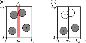
Figure 6: Vertical rift $[x_{r},x_{r}+\epsilon]\times[0,L_{y}]$. (a): $L_{x}\times L_{y}$ box with vertical rift of width $\epsilon$ at position $x_{r}$. (b): Transformed sample, which is eliminated because of a pair overlap.

The pressure can be estimated for finite $\epsilon$ from a finite number of samples, but then requires an extrapolation towards $\epsilon\to 0$. In EDMD and ECMC, the extrapolation can be avoided because of the infinite number of samples produced in a given run-time interval $\tau_{\text{sim}}$.

We first reduce the volume $V$ of a non-periodic $L_{x}\times L_{y}$ box by a vertical wall rift with $x_{r}=L_{x}-\epsilon$ or by a horizontal wall rift with $y_{r}=L_{y}-\epsilon$. A sample in the original box is eliminated through the wall rift with the probability that one of the disks overlaps the wall rift. Disk $i$ is at position $\mathbf{x}_{i}$ with the normalized single-disk probability density $\pi^{(1)}(\mathbf{x}_{i})$ and at an $x$-position in the interval $[L_{x}-\sigma-\epsilon,L_{x}-\sigma]$ with probability $\epsilon\int\mathrm{d}y\pi^{(1)}(L_{x}-\sigma,y)$. We normalize the single-disk density $\rho$ to $V$, so that the normalized probability density $\pi^{(1)}(\mathbf{x}_{i})$ of a given disk $i$ to be at position $\mathbf{x}_{i}$ equals $\pi(\mathbf{x}_{i})=\rho(\mathbf{x}_{i})/V$. We then use the rescaled line density $\rho_{x}(x)=\int\mathrm{d}y\rho(x,y)/L_{y}$, and likewise for $\rho_{y}(y)$. With the vertical rift volume $\epsilon L_{y}$ and analogously for the horizontal one, this gives the wall-rift pressure estimator:

$$\beta\left[\begin{array}[]{l}P_{x}\\ P_{y}\end{array}\right]=\frac{N}{V}\left[\begin{array}[]{l}\rho_{x}(L_{x}-\sigma)\\ \rho_{y}(L_{y}-\sigma)\end{array}\right].$$ (12)

Naively, the rescaled line densities $\rho_{x}$ and $\rho_{y}$ are obtained from a histogram of the $x$-coordinates, extrapolated to $x=L_{x}-\sigma$ and equivalently, to $x=\sigma$ (see Table 1, line 1 and Appendix A).

#	Sampling method: pressure estimator	$\beta P$
1	EDMD: wall-rift fit (see Eq. (12))	$10.74(7)$
2	EDMD: wall rift (see Eq. (13c))	$10.79625(4)$
3	ECMC: wall rift (see Eq. (14))	$10.7962(4)$
4	EDMD: rift average (see Eq. (19a))	$10.79629(3)$
5	ECMC: rift average (see Eq. (20))	$10.7962(4)$
6	EDMD: homothetic fit (see Eq. (27a))	$10.74(4)$

Table 1: Thermodynamic pressure estimates for four disks of radius $\sigma=0.15$ in a non-periodic square box of sides $1$. The kinematic estimators of Subsection III.3.3 lead to identical expressions.

Within EDMD, the rescaled line densities of Eq. (12) can be computed, without extrapolation, from the time interval $\Delta t=2\epsilon/|v^{\perp}_{\text{wall}}|$ before and after the collision during which a disk with perpendicular velocity $v^{\perp}_{\text{wall}}$ overlaps with the wall rift at $x_{r}=L_{x}-\epsilon$. The time interval $\Delta t$ here simply indexes equilibrium samples and has no kinematic meaning. The change of volume (by the two rifts at $x=0$ and $x=L_{x}$) equals $2\epsilon L_{y}$. For $\epsilon\to 0$, only a single disk overlaps with the wall rift, leading to the EDMD wall-rift estimator:

$$\beta P_{x} =\frac{1}{2L_{y}\tau_{\text{sim}}}\sum_{w:(i,\pm\hat{\mathbf{e}}_{x})}\frac{2}{|v^{\perp}_{(i)}|}\quad$$ (13a)

$$=\left\langle\frac{2}{|v^{\perp}_{\text{wall}}|}\right\rangle\overbrace{\frac{1}{2L_{y}\tau_{\text{sim}}}\sum_{w:(i,\pm\hat{\mathbf{e}}_{x})}1}^{\hat{n}_{\text{wall}}^{\pm\hat{\mathbf{e}}_{x}}}$$ (13b)

$$=\frac{2\sqrt{\pi}}{\sqrt{\sum v_{i}^{2}}}\frac{\Gamma(N+\frac{1}{2})}{\Gamma(N)}\hat{n}_{\text{wall}}^{\pm\hat{\mathbf{e}}_{x}}$$ (13c)

$$\stackrel{{\scriptstyle N\to\infty}}{{\longrightarrow}}\sqrt{2\pi\beta m}\hat{n}_{\text{wall}}^{\pm\hat{\mathbf{e}}_{x}}.$$ (13d)

The sum in Eq. (13a) goes over the wall collisions $w$ of all disks $i$ in $\pm\hat{\mathbf{e}}_{x}$ direction, and $\hat{n}_{\text{wall}}^{\pm\hat{\mathbf{e}}_{x}}$ is the wall-collision rate per vertical unit line element. In Eq. (13), the right-hand sides are estimators, whose expectation yields the pressure on the left-hand side. In this equation and the following ones, the additional $\left\langle\dots\right\rangle$ (such as $\hat{n}_{\text{wall}}^{\pm\hat{\mathbf{e}}_{x}}\to\left\langle\hat{n}_{\text{wall}}^{\pm\hat{\mathbf{e}}_{x}}\right\rangle$ in Eqs (13c) and (13d)) are omitted. In Eq. (13a), the estimator has infinite variance. It is regularized through its mean value in Eq. (13b). The latter is evaluated in Eq. (13c) with the Maxwell-boundary expression of Eq. (8), and tested to $4\!\times\!10^{-6}$ in relative precision against other estimators (see Table 1, line 2). The pressure estimator of Eq. (13c) can also be derived as a kinematic pressure estimator through the momentum transfer with the walls (see Subsection III.3.3). Thermodynamic and kinematic pressures thus agree already at finite $N$.

The wall-rift pressure estimator adapts non-trivially to ECMC. We consider straight ECMC with a single active disk that moves with unit speed along the $\pm\hat{\mathbf{e}}_{x}$ direction. As a lifted Markov chain, ECMC splits the equilibrium probability of each “collapsed” sample $\mathbf{x}$ equally between the $N$ lifted copies (consisting of $\mathbf{x}$ and of the label of the active disk for a given displacement vector) (see [52] and [58, Appendix A]). ECMC only determines overlaps with the walls for the active disk, and a lifted sample that must be eliminated is detected with a biased probability $1/N$. This bias is corrected by multiplying the right-hand side of Eq. (13a) by $N$, resulting in the ECMC wall-rift estimator:

$$\beta P_{x}=\frac{N}{2L_{y}\tau_{\text{sim}}}\sum_{w:(a,\pm\hat{\mathbf{e}}_{x})}\frac{2}{|v^{\perp}_{\text{wall}}|}=2N\hat{n}_{\text{wall}}^{\pm\hat{\mathbf{e}}_{x}}$$ (14)

(see Fig. 7a). It is tested to $4\!\times\!10^{-5}$ in relative precision (see Table 1, line 3).

Within molecular dynamics and ECMC, pressures can also be estimated by rifts inside the box and in particular by averages over all rift positions $x_{r}$ in addition to the average over $\tau_{\text{sim}}$ already contained in the wall-rift estimators. This can be written as

$$\beta P_{x}=\frac{1}{\epsilon L_{y}}\frac{1}{L_{x}\tau_{\text{sim}}}\int_{t}^{t+\tau_{\text{sim}}}\mathrm{d}\tau\int_{0}^{L_{x}-\epsilon}\mathrm{d}x_{r}\Theta(\tau,x_{r}),$$ (15)

where $\Theta(\tau,x_{r})$ is zero if the sample at time $t+\tau$ is maintained after the reduction with parameter $x_{r}$ and one if it is eliminated. The ideal-gas contribution to Eq. (15),

$$\beta P_{x}^{\text{ideal gas}}=\frac{\epsilon N}{L_{x}}\frac{1}{\epsilon L_{y}}=\frac{N}{V},$$ (16)

counts the proportion of rifts that eliminate samples because the centers of the disks fall inside. The pair-collision contribution to Eq. (15) is derived considering the sample shown in Fig. 6. If the distance between two disks $i$ and $j$ is in the interval $[2\sigma,2\sigma+\epsilon\Delta x^{\min}_{ij}/(2\sigma)]$, where $\Delta x^{\min}_{ij}$ is the $x$-separation at contact, the corresponding samples are eliminated for a time $(2/|\Delta v^{\perp}_{ij}|)[\epsilon\Delta x^{\min}_{ij}/(2\sigma)]$ for vertical rifts in the interval of length $\Delta x^{\min}_{ij}$ between the two disks at contact. Together with the wall term analogous to Eq. (13), the rift-average pressure estimator for EDMD thus reads:

$$\beta P_{x}=\frac{N}{V}+\frac{1}{V\tau_{\text{sim}}} \left[\sum_{p:(ij)}\frac{|\Delta x^{\min}_{ij}|^{2}}{2\sigma}\right.\left\langle\frac{2}{\Delta v^{\perp}_{ij}}\right\rangle$$

$$\left.+\sum_{w:(i,\pm\hat{\mathbf{e}}_{x})}\left\langle\frac{2\sigma}{|v^{\perp}_{\text{wall}}|}\right\rangle\right],$$ (17)

where the mean values again involve Maxwell-boundary expressions. Eq. (17) can be combined with an analogous expression for $P_{y}$ to obtain the EDMD rift-average estimator for $P$:

$$\beta P=\frac{N}{V}+\frac{\sigma}{V\tau_{\text{sim}}}\left[\sum_{p:(ij)}\right. \left\langle\frac{2}{\Delta v^{\perp}_{ij}}\right\rangle$$

$$\left.+\sum_{w:(i,\pm\hat{\mathbf{e}}_{x},\pm\hat{\mathbf{e}}_{y})}\left\langle\frac{1}{|v^{\perp}_{\text{wall}}|}\right\rangle\right].$$ (18)

In a non-periodic box, using Eqs (8) and (9), the EDMD rift-average estimator takes the form

$$\beta P =\frac{N}{V}+\frac{\sigma\sqrt{\pi}}{\sqrt{\sum v_{i}^{2}}V}\frac{\Gamma(N+\frac{1}{2})}{\Gamma(N)}(n_{\text{wall}}^{\pm\hat{\mathbf{e}}_{x}\pm\hat{\mathbf{e}}_{y}}+\sqrt{2}n_{\text{pair}})$$ (19a)

$$\stackrel{{\scriptstyle N\to\infty}}{{\longrightarrow}}\frac{N}{V}\left(1+\frac{\sigma\sqrt{\pi m\beta}}{N}n_{\text{pair}}\right),$$ (19b)

where $n_{\text{wall}}^{\pm\hat{\mathbf{e}}_{x}\pm\hat{\mathbf{e}}_{y}}$ is the wall-collision rate, the number of all wall collisions per time interval, and similarly for the pair-collision rate $n_{\text{pair}}$. In the $N\to\infty$ limit of Eq. (19b), wall collision play no role. The EDMD rift-average estimator of Eq. (19a) is tested to $3\!\times\!10^{-6}$ in relative precision (see Table 1, line 4).

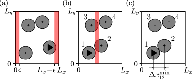
Figure 7: ECMC rift estimators. (a): The ECMC wall-rift estimator only detects rift overlaps of the active disk, explaining the factor $N$ in Eq. (14), that is absent in Eq. (13a). (b): A pair of disks $(i,j)$ leading to the elimination of the sample is detected only if either $i$ or $j$ are active, explaining a factor $N/2$ entering Eq. (20). (c): Illustration of the $x$-separation at contact $\Delta x^{\min}_{ij}$ (also relevant for EDMD).

Rift-average pressure estimators for ECMC detect wall and pair collisions with biases (see Eq. (14)), that must again be corrected, namely by a factor $N$ for each wall event and by a factor $N/2$ for each pair event, the latter because a lifted sample of $N$ disks that must be eliminated is detected only if either $i$ or $j$ are active (see Fig. 7c). This leads to the straight-ECMC rift-average estimator,

$$\beta P_{x}=\frac{N}{V}+\frac{N}{V\tau_{\text{sim}}}\left(\sum_{p:(ij)}\Delta x^{\min}_{ij}+\sum_{w:(i\pm\hat{\mathbf{e}}_{x})}2\sigma\right),$$ (20)

that again differs in the factors $\propto N$ from the corresponding formulas of EDMD. Furthermore, it averages over a bounded distribution of $\Delta x^{\min}_{ij}$, with the wall-velocity only taking the values $\pm 1$, whereas in EDMD, the corresponding continuous distributions of $1/|\Delta v^{\perp}_{ij}|$ and of $1/|v^{\perp}_{\text{wall}}|$ have infinite variance. The straight-ECMC estimator of Eq. (20) is tested to $4\!\times\!10^{-5}$ in relative precision (see Table 1, line 5).

In a periodic box, there are no wall collisions, and the direction of motion of straight ECMC is either $+\hat{\mathbf{e}}_{x}$ or $+\hat{\mathbf{e}}_{y}$. In Eq. (20), all the $x$-separations at contact $\Delta x^{\min}_{ij}$ and the chain length $\tau_{\text{sim}}$ (which, because of the unit velocity, corresponds to the total displacement) add up to the difference of the final position $x_{\text{final}}$ of the last disk of the chain and the initial position $x_{\text{initial}}$ of the chain’s first disk. Here, periodic boundary conditions are accounted for, so that in the absence of collision, this distance equals $\tau_{\text{sim}}$. For an event chain in the $+\hat{\mathbf{e}}_{x}$ direction, Eq. (20) thus simplifies into the straight-ECMC estimator for a periodic box [41]:

$$\beta P_{x}=\frac{N}{V\tau_{\text{sim}}}(x_{\text{final}}-x_{\text{initial}}),$$ (21)

that is easy to compute, and that will be used extensively in Section IV. There, we alternate event chains in $+\hat{\mathbf{e}}_{x}$, which estimate $P_{x}$, and event chains in $+\hat{\mathbf{e}}_{y}$, which estimate $P_{y}$. Alternating the direction of straight-ECMC chains is required for convergence towards equilibrium. The rift-average estimator generalizes to other variants of ECMC. The pressure $P_{y}$ can also be estimated through event chains in $\pm\hat{\mathbf{e}}_{x}$ and horizontal-rift averages, leading for the straight ECMC in $+\hat{\mathbf{e}}_{x}$ to:

$$\beta P_{y}=\frac{N}{V}+\frac{N}{V\tau_{\text{sim}}}\sum_{p:(ij)}\frac{|\Delta y^{\min}_{ij}|^{2}}{\Delta x^{\min}_{ij}}.$$ (22)

However, this estimator has infinite variance and is less convenient than Eq. (21).

III.3.2 Homothetic volume reductions

Besides by rifts, the volume $V$ of an $L_{x}\times L_{y}$ box can be reduced by a homothetic transformation, where the box and all positions $\mathbf{x}_{i}$ are homogeneously scaled by a factor $1-\epsilon_{\alpha}<1$, while the disk radii $\sigma$ remain unchanged. The transformation of the box corresponds to simultaneous horizontal and vertical rifts of equal rift volume, but the disk positions then transform inhomogeneously, as in Eq. (11).

A homothetic volume reduction yields the pressure $\beta P=\beta(P_{x}+P_{y})/2$, rather than one of the components. It may be performed in two steps. In a first step (from $(\sigma,V)$ to $(\sigma^{\prime},V)$, see Fig. 8), the box and the $\mathbf{x}_{i}$ are unchanged, but the disks are swollen by a factor $1/(1-\epsilon_{\alpha})$, possibly eliminating samples. In a second step, all lengths are rescaled by $1-\epsilon_{\alpha}$, so that the radii return to $\sigma$. This second step (from $(\sigma^{\prime},V)$ to $(\sigma,V^{\prime})$) is rejection-free, and its reduction of sample-space volume, with $Z(\sigma,V^{\prime})=(V^{\prime}/V)^{N}Z(\sigma^{\prime},V)$, constitutes the ideal-gas term of the pressure.

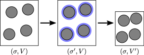
Figure 8: A homothetic volume reduction performed through a swelling of disks followed by a uniform reduction of all lengths (box, positions, radii).

In the two-stage transition $Z(\sigma,V)\to Z(\sigma^{\prime},V)\to Z(\sigma,V^{\prime})$, the two-step procedure turns Eq. (10) into

$$\beta P\stackrel{{\scriptstyle V^{\prime}\to V}}{{=}} \frac{\log\left[Z(\sigma,V)\right]-\log\left[Z(\sigma,V^{\prime})\right]}{V-V^{\prime}}$$ (23)

$$= \frac{N}{V}+\frac{1}{V-V^{\prime}}\frac{Z(\sigma,V)-Z(\sigma^{\prime},V)}{Z(\sigma,V)}.$$

The final term again divides the elimination probability of a sample by the change of volume (see also [59, 60, 61, 62]).

The pair-elimination probability is expressed by the normalized probability density $\hat{g}(r_{x},r_{y})$, with $\hat{g}(r_{x},r_{y})\mathrm{d}r_{x}\mathrm{d}r_{y}$ the probability that a that a given pair distance is in $[r_{x},r_{x}+\mathrm{d}x][r_{y},r_{y}+\mathrm{d}y]$. With $\hat{g}(r)$ as the average of $\hat{g}(r_{x},r_{y})$ over the corresponding ring of radius $r$, the probability that a given pair distance is in the interval $[r,r+\mathrm{d}r]$ is thus $2\pi r\hat{g}(r)\mathrm{d}r$. By convention, the pair correlation function $g(r)$ is normalized to $g(r)=V\hat{g}(r)$. For our application, we have $r=2\sigma$ and $\mathrm{d}r=2\sigma\epsilon_{\alpha}$, and there are $N(N-1)/2$ pairs of disks. Also, the absolute change of volume for $L_{x}\to L_{x}(1+\epsilon_{\alpha})$ and $L_{y}\to L_{y}(1+\epsilon_{\alpha})$ is $2V\epsilon_{\alpha}$. The pair-collision contribution to the pressure is thus:

$$\beta P^{\text{pair}}=\frac{N}{V}\frac{N-1}{V}2\pi\sigma^{2}g(2\sigma),$$ (24)

an expression that is correct for finite $N$ and in periodic or non-periodic boxes. The extrapolation of $g(2\sigma)$ from a histogram is detailed in Appendix A. The range of distances to the wall that are eliminated is $[\sigma,\sigma(1+\epsilon_{\alpha})]$, and the change in volume remains $2\epsilon_{\alpha}V$. The contribution to the pressure of the wall at $x=0$ is then

$$\beta P^{\text{wall},-\hat{\mathbf{e}}_{x}}=\frac{N\sigma\epsilon_{\alpha}}{2\epsilon_{\alpha}V}\int\mathrm{d}y\pi(\sigma,y)=\frac{N\sigma}{2VL_{x}}\rho_{x}(\sigma).$$ (25)

where we used the rescaled line densities $\rho_{x}$ and $\rho_{y}$ which remain $\mathcal{O}\left(1\right)$ for $V\to\infty$ (see Subsection III.3.1). Summing over the four wall terms, one arrives at

$$\beta P^{\text{wall}}=\frac{N\sigma}{V}\left[\frac{\rho_{x}(\sigma)}{L_{x}}+\frac{\rho_{y}(\sigma)}{L_{y}}\right].$$ (26)

The computation of the line densities $\rho_{x}(\sigma)$ and $\rho_{y}(\sigma)$ from a histogram is detailed in Appendix A. The combined pair and wall contributions yield the homothetic pressure estimator for a non-periodic $L_{x}\times L_{y}$ box:

$$\beta P=N/V+$$

$$\frac{N}{V}\left[2\pi\frac{(N-1)\sigma^{2}}{V}g(2\sigma)+\sigma\frac{\rho_{x}(\sigma)}{L_{x}}+\sigma\frac{\rho_{y}(\sigma)}{L_{y}}\right]$$ (27a)

$$\stackrel{{\scriptstyle N\to\infty}}{{\longrightarrow}}\frac{N}{V}\left[1+2\eta g(2\sigma)\right].$$ (27b)

Eq. (27a) is tested by histogram fits and extrapolations to contact of $\rho(\sigma)$ and $g(2\sigma)$ to $4\!\times\!10^{-3}$ in relative precision (see Table 1, line 6). Eq. (27b) has long been used for estimating pressures in MCMC [28].

EDMD and ECMC can estimate the pressure without the extrapolations of the pair correlation functions and the wall densities by tracking the time during which pairs of disks are close to contact, or a disk is close to the wall. The explicit computation for EDMD simply reproduces Eqs (18) and (19), both at finite $N$ and in the thermodynamic limit. The corresponding homothetic pressure estimators for ECMC are readily derived, but they have diverging variances that require specific care. For all variants except straight ECMC, they correctly estimate wall contributions to the pressure and can be used for non-periodic boxes. The velocities of straight ECMC are always parallel to some walls, precluding the estimation of all wall contribution to the pressure.

III.3.3 Kinematic pressure estimators

Kinematic pressure estimators of EDMD determine the time-averaged exchange of momentum between disks, or between disks and a wall. Their use goes back to Daniel Bernoulli [16], who pointed out that under the scaling $\mathbf{v}_{i}\to\gamma\mathbf{v}_{i}\forall i$ of Eq. (2), both the number of collisions per time interval and the momentum transmitted scaled as $\gamma$, so that the pressure had to be proportional to the square of the (mean) velocity (in other words to the temperature). In the non-periodic $L_{x}\times L_{y}$ box, the transmitted momentum with, say, the vertical walls at $x=0$ and $x=L_{x}$ gives the kinematic EDMD estimator:

$$P_{x} =\frac{1}{2L_{y}\tau_{\text{sim}}}\sum_{w:(i,\pm\hat{\mathbf{e}}_{x})}2m|v^{\perp}_{\text{wall}}|$$ (28a)

$$=2m\left\langle|v^{\perp}_{\text{wall}}|\right\rangle\hat{n}_{\text{wall}}^{\pm\hat{\mathbf{e}}_{x}}$$ (28b)

$$=\frac{mR_{v}\sqrt{\pi}}{N}\frac{\Gamma(N+\frac{1}{2})}{\Gamma(N)}\hat{n}_{\text{wall}}^{\pm\hat{\mathbf{e}}_{x}},$$ (28c)

$$\stackrel{{\scriptstyle N\to\infty}}{{\longrightarrow}}\sqrt{2\pi\beta m}\hat{n}_{\text{wall}}^{\pm\hat{\mathbf{e}}_{x}},$$ (28d)

where in Eq. (28c), we used Eq. (8b). Already at finite $N$, the kinematic EDMD estimator of Eq. (28c) is identical to the thermodynamic wall-rift pressure estimator of Eq. (13c), as we may identify $R_{v}^{2}=2N/(m\beta)$.

The EDMD kinetic pressure estimator can also be derived from the virial function

$$G_{x}=m\sum_{i=1}^{N}x_{i}v_{i,x}$$ (29)

which is strictly bounded during molecular dynamics, so that its mean time derivative vanishes:

$$\left\langle\frac{\mathrm{d}missing}{\mathrm{d}t}G_{x}\right\rangle=\left\langle\frac{\mathrm{d}missing}{\mathrm{d}t}G_{x}^{\text{wall}}\right\rangle+\left\langle\frac{\mathrm{d}missing}{\mathrm{d}t}G_{x}^{\text{pair}}\right\rangle+m\left\langle\sum_{i=1}^{N}v_{i,x}^{2}\right\rangle\\ =m\left\langle\sum_{i=1}^{N}(x_{i}\dot{v}_{i,x}+v_{i,x}^{2})\right\rangle=0.$$ (30)

The wall contribution to this expression stems from collisions with the vertical walls at $x=0$ and $x=L_{x}$, which are given by $2m\left\langle|v^{\perp}_{\text{wall}}|\right\rangle\sigma$ and $-2m\left\langle|v^{\perp}_{\text{wall}}|\right\rangle(L_{x}-\sigma)$, respectively. This results in

$$\left\langle\frac{\mathrm{d}missing}{\mathrm{d}t}G_{x}^{\text{wall}}\right\rangle =-2m\left\langle|v^{\perp}_{\text{wall}}|\right\rangle(L_{x}/2-\sigma)n_{\text{wall}}^{\pm x}$$ (31a)

$$=-VP_{x}+2m\sigma\left\langle|v^{\perp}_{\text{wall}}|\right\rangle 2L_{y}\hat{n}^{\pm x}_{\text{wall}},$$ (31b)

where we have used Eq. (28b).

For the pair-collision contribution to Eq. (30), we use that at the collision of disks $i$ and $j$, the distance $\Delta\mathbf{x}_{ij}=\mathbf{x}_{i}-\mathbf{x}_{j}$ satisfies $|\Delta\mathbf{x}_{ij}|=2\sigma$. With the unit vector $\hat{\mathbf{e}}_{\perp}=\Delta\mathbf{x}_{ij}/(2\sigma)$ and the velocity difference $\Delta\mathbf{v}=\mathbf{v}_{i}-\mathbf{v}_{j}$ (before the collision), the change of the velocity of disk $i$ is $-\hat{\mathbf{e}}_{\perp}(\Delta\mathbf{v}\boldsymbol{\cdot}\hat{\mathbf{e}}_{\perp})$, and the change of the velocity of disk $j$ is $\hat{\mathbf{e}}_{\perp}(\Delta\mathbf{v}\boldsymbol{\cdot}\hat{\mathbf{e}}_{\perp})$ (see [39, Sect. 2.1.1]). An individual pair collision thus contributes

$$-m\frac{(\Delta x^{\min}_{ij})^{2}}{4\sigma^{2}}\underbrace{(\Delta\mathbf{v}\boldsymbol{\cdot}\Delta\mathbf{x}_{ij}^{\text{min}})}_{-2\sigma|\Delta v^{\perp}_{ij}|},$$ (32)

an expression where both terms can be averaged independently. Finally, we may use $\left\langle v_{i,x}^{2}\right\rangle=R_{v}^{2}/(2N)$ to rearrange Eq. (30) into a kinematic EDMD pressure estimator:

$$\beta P_{x}=\frac{N}{V}+\frac{\beta}{V\tau_{\text{sim}}}\sum_{w:(i,\pm\hat{\mathbf{e}}_{x})}\left\langle 2\sigma|v^{\perp}_{\text{wall}}|\right\rangle\\ +\sum_{p:(ij)}\frac{(\Delta x^{\min}_{ij})^{2}}{4\sigma^{2}}\left\langle 2\sigma\Delta v^{\perp}_{ij}\right\rangle.$$ (33)

Using Eqs (8) and (9), this kinematic estimator is seen to be equivalent to the thermodynamic rift-average estimator of Eq. (17).

IV Equation-of-state computations

We now compare historic hard-disk pressure computations since 1953 [28, 63, 64, 65, 66, 14, 49, 67] with massive simulation results obtained in this work using the sampling algorithms and pressure estimators of Section III. Our re-evaluation will illustrate the three principal challenges that the hard-disk model shares, mutatis mutandis, with other sampling problems. First, the estimate of the pressure continues to depend on the initial configuration for very long run times, until equilibrium is reached. We will call this time the “mixing time” [47] in a slight abuse of terminology, as we do not consider certain pathological initial configurations, which trap the Markov chain forever (see [53]). The pioneering works, by Metropolis et al. and by Alder and Wainwright obtained crucial insights from very short computer experiments with run times much below the mixing time. However, later works that attempted to interpret manifestly unequilibrated samples [68, 69, 70], or that failed to recognize the lack of convergence, arrived at qualitatively wrong conclusions. In the hard-disk model, mixing times can be bounded rigorously only at small densities [71]. At higher densities, heuristic criteria for the mixing time, which have not been fully presented before, appear crucial. In our case, they depend on time series of other observables than the pressure, or on multiple runs from qualitatively different initial configurations.

The second challenge for hard-disk computations consists in the intricate dependence of the pressure on the shape of the box (that is, the aspect ratio) and on the number $N$ of disks, rendering extrapolations to the thermodynamic limit non-trivial. In small boxes, the hexatic and solid phases are confounded, as they only differ at large distances, so that the behavior in the thermodynamic limit is not necessarily reflected in the equation of state at small $N$.

The third challenge concerns the very evaluation of the pressure. Within Monte Carlo methods, the pressure was long evaluated through extrapolation towards contact of the pair correlation function in Eq. (27b), a procedure fraught with uncertainty. The rift formulas of Subsection III.3 that originated with ECMC, and that we even use in MPMC as short fictitious ECMC runs placed at regular time intervals, overcome the need for extrapolations.

IV.1 Hard-disk equation of state for small $N$

Since the early days of computer simulation, the pressure of the hard-disk model has been computed with the aim of determining its phase behavior in the thermodynamic limit. While the identification of thermodynamic phases in finite systems can be subject to discussion, the pressure is unambiguously defined, and it can in principle be computed to arbitrary precision.

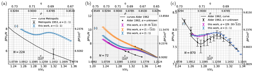
Figure 9: Equations of state $P(V)$ for the hard-disk model at small $N$. (a): $P(V)$ for $N=244$ for $\alpha\!=\!(1\!:\!1)$ computed in 1953 [28] compared with ECMC computations (this work). (b): $P(V)$ for $N=72$ computed in 1962 [14] (for unspecified aspect ratio $\alpha$) and ECMC pressures for $\alpha\!=\!(1\!:\!\sqrt{3}/2)$, $(1\!:\!1)$, and $(9\!:\!8\sqrt{3}/2)$. (c): $P(V)$ for $N=870$. This work’s square-box computations satisfy $\left\langle\Psi_{6}\right\rangle\simeq 0$, except for data points in parentheses (see Fig. 10).

IV.1.1 Metropolis et al. (1953), rotation criterion

In $1953$, in the publication that first introduced MCMC, Metropolis et al. [28] estimated the pressure from the extrapolated pair-correlation function for $224$ disks in a periodic square box. This number $224=16\times 14$ disks can be perfectly packed at density $\eta=\pi/(2\sqrt{3})=0.907$ in an almost square-shaped box of aspect ratio $\alpha\!=\!(16\sqrt{3}/2\!:\!14)=(0.9897\!:\!1)$ and almost at that density in a perfectly square box. Metropolis et al. concluded that “(t)here is no indication of a phase transition”. The equation of state for $N=224,\alpha\!=\!(1\!:\!1)$, recomputed in this work using straight ECMC to a relative precision of $10^{-4}$, is somewhat higher than the historic pressures. It is also slightly non-monotonic (see Fig. 9a).

The $224$-disk square-box system of Metropolis et al., from $1953$, carries lessons that are pertinent to the present day. Indeed, in a square box, any hard-disk sample can be rotated by an angle $\pi/2=90$° into another valid sample. At high enough density, two such samples are inequivalent because the local hexagon which describes the six disks that typically surround any given disk has on average a $60$° symmetry but not a $90$° symmetry. For each local set of samples, there thus exists another inequivalent set of samples (generated through a $90$° rotation) of identical statistical weight. This rotation, and the corresponding transformation of samples can be formalized through the global orientational order parameter

$$\Psi_{6}=\frac{1}{N}\sum_{l}\frac{1}{\text{nbr}(l)}\sum_{j=1}^{\text{nbr}(l)}e^{6i\phi_{lj}},$$ (34)

that changes from $\Psi_{6}$ to $-\Psi_{6}$ (that is, $\arg(\Psi_{6})\to\arg(\Psi_{6})+\pi$) under a rotation by $90$°. In Eq. (34), $\phi_{lj}$ is the angle of the line connecting disks $l$ and $j$ with respect to the $\hat{\mathbf{e}}_{x}$-axis, and $\text{nbr}(l)$ is the number of neighbors of $l$ resulting from a Voronoi construction. In a square box, the ensemble average of the orientational order parameter thus satisfies $\left\langle\Psi_{6}\right\rangle=0$, and for an irreducible Markov chain, it agrees with its time average, as expressed in the ergodic theorem [47]:

$$\mathbb{P}_{\pi^{\{0\}}}\left[\lim_{t\to\infty}\frac{1}{t}\sum_{i=1}^{t}f_{i}=\left\langle f\right\rangle\right]=1,$$ (35)

where $f$ is a function of the sample at time $i$ given the distribution $\pi^{\{0\}}$ of initial configurations, and $\mathbb{P}$ is the probability. As the mean value $\left\langle\Psi_{6}\right\rangle$ is known to vanish, we can employ Eq. (35) with $f=\Psi_{6}$ as a diagnostic tool and suppose that the hard-disk Markov chain in a square box reaches the mixing time (with errors decreasing as the square root of the run time) only when the orientational order parameter $\Psi_{6}$ has been rotated by more than $180$° :

$$|\text{supp}(\arg(\Psi_{6})|>\pi.$$ (36)

Here, “supp” stands for the support of the empirical distribution, in our case for the range of angles of $\Psi_{6}$ that are visited during a simulation. This heuristic rotation criterion supposes that the orientational order parameter $\Psi_{6}$ is the slowest-decaying variable in the hard-disk system. Our time series of $\Psi_{6}$ in a square box, with known mean value $\left\langle\Psi_{6}\right\rangle=0$, pinpoints problems with a hard-disk pressure estimation that might not be signaled by the time series of the pressure itself. We use the rotation criterion in two different settings. In small systems (as the $224$-disk case of Metropolis et al.), the entire range of $\arg(\Psi_{6})$ values is swept through many times, leading to high-precision estimates for the pressure, even though it strongly depends on the angle. In large systems, as the hard-disk model with $N=128^{2}$ at $\eta=0.716$, that we will discuss in Fig. 12, we barely satisfy the criterion, but it still assures us that up to a symmetry $\Psi_{6}\to-\Psi_{6}$ all relevant regions of sample space were visited. High-precision estimates for the pressure now result from the fact that the pressure depends weakly on $\arg(\Psi_{6})$.

Our ECMC simulations satisfy the rotation criterion for $N=224$ in a periodic square box up to a density $\eta=0.72$. At large enough densities, the ECMC simulation may remain for long times in a set of samples with essentially the same value of $\arg(\Psi_{6})$ before flipping to another set of samples with $\arg(\Psi_{6})+\pi$. This very slow rotation of $\Psi_{6}$ is a harbinger of the serious convergence problems of the hard-disk model for larger $N$ at densities of physical interest. As we will show, the pressure is strongly correlated with $\Psi_{6}$ up to moderate values of $N$.

IV.1.2 Revisiting Alder and Wainwright (1962)

Alder and Wainwright, in $1962$, used EDMD to estimate the pressure for $72$ and $870$ disks in rectangular periodic boxes for which they did not specify the aspect ratios. As already discussed in Fig. 1, their non-monotonic equation of state led to the prediction of a phase transition. The computed pressure is independent of the sampling method (molecular dynamics, local Metropolis algorithm, ECMC), but it depends on the aspect ratio of the box. For $72=9\times 8$ disks and aspect ratio $\alpha\!=\!(9\!:\!8\sqrt{3}/2)=(1\!:\!0.7698)$ where they can be perfectly packed, the equation of state obtained by ECMC in this work agrees remarkably well with the historic data (see Fig. 9b). In contrast, for a square box (aspect ratio $\alpha\!=\!(1\!:\!1)$), the equation of state follows a slight “S” shape, but it remains monotonous for all densities. For the aspect ratio $\alpha\!=\!(1\!:\!\sqrt{3}/2)$, the pressure is barely “S” shaped. For the aspect ratio $\alpha\!=\!(1\!:\!1)$, our ECMC computations satisfy the rotation criterion up to densities $\eta\lesssim 0.74$, and pressure estimates achieve $10^{-4}$ relative precision.

For $870$ disks, the dependence of the pressure on the aspect ratio is less pronounced than for $N=72$ (see Fig. 9c). Since $870=30\times 29$, this number of disks can be close-packed for the aspect ratio $\alpha\!=\!(29\!:\!30\sqrt{3}/2)=(1\!:\!0.896)$. For the aspect ratio $\alpha\!=\!(1\!:\!1)$, the orientation criterion of Eq. (36) is again satisfied up to high densities (see Fig. 10a). However, even at moderate densities, an ECMC run can take several CPU hours before visiting all possible orientations, and the pressure clearly correlates with the orientation (see Fig. 10b). On smaller time scales, the time series remains blocked in samples that all roughly have the same orientational order parameter $\Psi_{6}$ (see Fig. 10c). Analyzing such shorter time series gives incorrect estimates of the pressure ($P_{\alpha}$ or $P_{\beta}$, etc., rather than $P$). Accordingly, the window-averaged pressure features long-time correlations, with an estimated autocorrelation time of $\sim 2\!\times\!10^{10}$ events (corresponding to roughly two CPU hours for ECMC). Nevertheless, on a long enough time scale estimated by the rotation criterion, all these systematic errors disappear, and the error of the pressure estimator starts to decrease as the square root of the run time (see Fig. 10d). The achieved $10^{-4}$ relative error on the pressure estimates in Fig. 9c, from longer simulations than those illustrated in Fig. 10, is much smaller than the systematic error $|\left\langle P_{\alpha}\right\rangle-\left\langle P_{\gamma}\right\rangle|/P\sim 10^{-2}$ of a calculation that is too short to rotate $\Psi_{6}$.

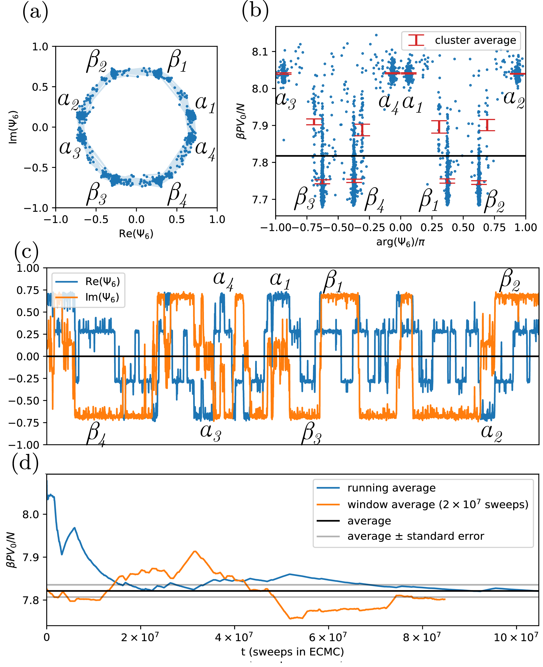
Figure 10: Pressure $P$ and global orientational order $\Psi_{6}$ for a three-hour ECMC run ($N=870$, $\eta=0.716$, square box $\alpha\!=\!(1\!:\!1)$). (a): Values of $\Psi_{6}$ in the complex plane. Highlighted clusters with inverted $\Psi_{6}$ (such as $\alpha_{1}$ and $\alpha_{3}$) have the same statistical weight. (b): Cluster averages for $P$ vs. $\arg(\Psi_{6})$. (c): Trajectories of $\text{Im}(\Psi_{6})$ and $\text{Re}(\Psi_{6})$ with indicated clusters. (d): Running average and window average for $P$.

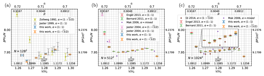
Figure 11: Equations of state $P(V)$ for the hard-disk model at large $N$. (a): $P(V)$ for $N=128^{2}$ from Refs [63, 73] and MPMC pressures (this work) for $\alpha\!=\!(1\!:\!\sqrt{3}/2)$ and $\alpha\!=\!(1\!:\!1)$ where all but the data point in parentheses satisfy the rotation criterion of Eq. (36) (see Fig. 12 for $\Psi_{6}$-resolved pressures). (b): $P(V)$ for $N=512^{2}$ from Refs [65, 66, 66, 49] and MPMC pressures (this work) for aspect ratios $\alpha\!=\!(1\!:\!\sqrt{3}/2)$ and $\alpha\!=\!(1\!:\!1)$, where runs with $\eta<0.712$ satisfy the rotation criterion. (c): $P(V)$ for $1024^{2}$ from Refs [66, 33, 49, 67], compared to MPMC (this work) for aspect ratios $\alpha\!=\!(1\!:\!\sqrt{3}/2)$ and $(1\!:\!1)$, where at density $\eta>0.708$ the rotation criterion is violated, but the systematic error thus committed is negligible (see Fig. 13a).

IV.2 Equations of state for large $N$

The equations of state for larger $N$ than those considered by Metropolis et al. and by Alder and Wainwright came into focus in the decades following 1962. At sufficiently large $N$, as we know today, fluid, hexatic, and solid phases can be distinguished, and the latter clearly differs from the crystal. In the simulations, three effects stand out. First, mixing and autocorrelation times become truly gigantic already for reasonable densities, even for the best currently known algorithms. Nevertheless, the pressure (as other physical quantities that we do not consider in this work) can be computed to a precision that, from a given time on, increases as the square root of the computer time. From $N=128^{2}$ to $N=1024^{2}$, this program can be put into practice, but it requires considerable computer resources. The failure to converge is signaled through a number of criteria, but not necessarily by the time series itself. Second, in the coexistence phase of the fluid and the hexatic in the $NVT$ ensemble, the initial dynamics towards equilibrium is dominated by coarsening. In this process, for example, small hexatic islands nucleate in the fluid, then coalesce and slowly grow until, in the stationary state of the time evolution, the sample presents itself as two domains, one for each coexisting phase. Precise knowledge of the pressure allows one to draw the boundaries of the phase coexistence. Third, as realized ten years ago, the high-density coexisting phase through the first-order phase transition is a hexatic, and thus distinct from the crystal that can serve as an initial configuration of MCMC configurations. Mixing times in the hexatic phase are very long, and are likely to scale with a larger exponent with $N$ than in the fluid [20].

IV.2.1 Hard-disk model with $N=128^{2}$ to $N=512^{2}$

For the hard-disk model with $N=128^{2}$, the relative precision levels of sequential ECMC, parallel ECMC, and of MPMC reach $\sim 10^{-5}$ for the pressure, for example, at $\eta=0.698$, much more precise than previous studies in the literature [63, 73] (see Fig. 11a). For $\alpha\!=\!(1\!:\!1)$, our calculations satisfy the rotation criterion of Eq. (36) up to density $\eta=0.716$, albeit for high densities on an impressive time scale, even for the MPMC algorithm (see Fig. 12). This is where earlier studies failed to equilibrate, and produced erroneous pressure estimates.

At density $\eta=0.716$, samples of the MPMC computation may remain in one cluster indexed by a given value of $\arg(\Psi_{6})$ for $\sim 10^{9}$ sweeps, and then produce a cluster average for the pressure $\beta PV_{0}/N$ that differs relatively by about $10^{-3}$ from the equilibrium average (see Fig. 12c). On such time scales, the outcome of the simulation is thus unpredictable, and the observed convergence of the pressure is not towards its ensemble average but towards some metastable cluster value. This behavior is readily detected from within the simulation data through the rotation criterion of Eq. (36) and through the dependence of obtained pressure values on initial conditions (such as different orientations or fluid and crystalline initial configurations).

For even larger systems, such as $N=512^{2}$, the computations in the literature dramatically suffer from the failure to equilibrate, with incorrect pressure estimates especially at high densities. For $\alpha\!=\!(1\!:\!1)$, our MPMC implementation satisfies the rotation criterion at $\eta\lesssim 0.712$ within a few weeks of computer time (which would correspond to centuries of run time of the local Metropolis algorithm on a single CPU). For even higher densities, all currently known sampling algorithm fail to equilibrate in the strict sense of that criterion. Fortunately, at larger $N$, the influence of the boundary conditions is much smaller than for small $N$ (see Fig. 13a). We estimate the systematic error stemming from the failure to rotate $\Psi_{6}$ by starting independent simulations for $N=512^{2}$ from a number of initial configurations with different global orientational order parameters $\Psi_{6}$ (see Fig. 13a). The resulting systematic errors are found to be at most as large as the statistical errors. Our pressure values are consistent with previous ECMC and MPMC calculations [33, 49] up to $\eta=0.718$, cross-validating the correctness of the conclusion in Ref. [49] (see Fig. 11b). In a non-square box, the components $P_{x}$ and $P_{y}$ of the pressure generally differ. For $N=128^{2}$ and $512^{2}$ at aspect ratio $\alpha\!=\!(1\!:\!\sqrt{3}/2)$, our estimates for $P_{x}$ and $P_{y}$ agree within error bars even in the hexatic phase, as the system dimensions are larger than the positional correlation length.

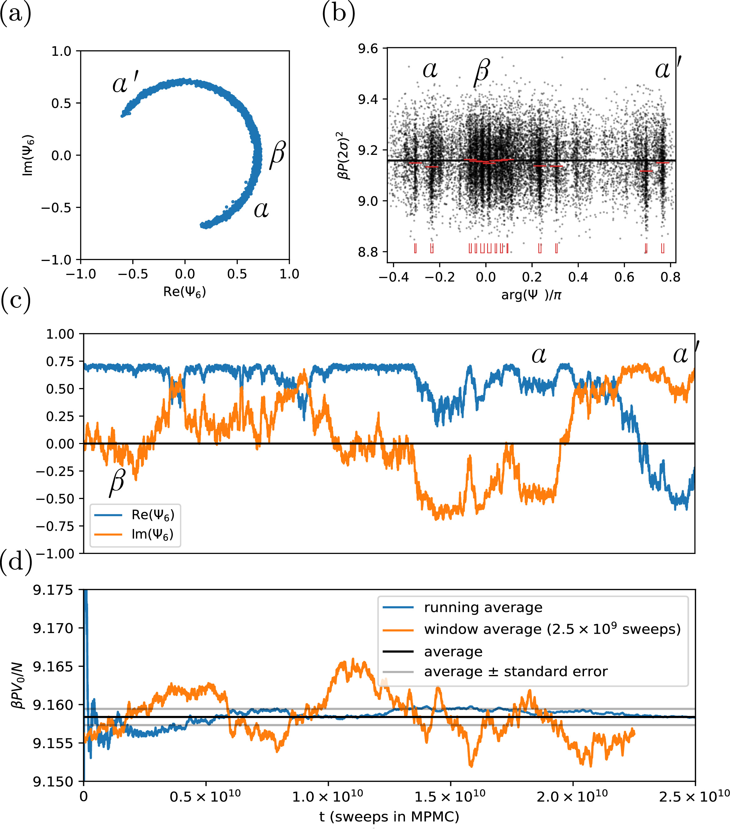
Figure 12: Analysis of the rotation criterion of Eq. (36) for a single MPMC run ($N=128^{2}$, $\eta=0.716$, $\alpha\!=\!(1\!:\!1)$). (a): Histogram of $\Psi_{6}$ in the complex plane. Clusters $\alpha$, $\alpha^{\prime}$ satisfies $\Psi_{6}^{\alpha}=-\Psi_{6}^{\alpha^{\prime}}$ and have equal weight. (b): Trajectory of $\text{Re}(\Psi_{6})$ and $\text{Im}({\Psi_{6}})$ with first visits to clusters indicated (cf Fig. 10). (c): Running average and window average of the pressure, showcasing slow convergence.

IV.2.2 Hard-disk model at $N=1024^{2}$

For the hard-disk model at $N=1024^{2}$, single-core implementations of the reversible Metropolis algorithm and of EDMD fail to equilibrate for densities $\eta\gtrsim 0.700$ on accessible time scales even on a modern CPU. Only straight ECMC (whose week-long mixing time of the serial version [33] reduces in the parallel implementation) and MPMC (run in parallel on thousands of cores on a GPU) are currently able to partially achieve convergence. It is for this reason that in the past, unconverged calculations [65, 66, 67] resulted in erroneous pressure estimates and, in consequence, qualitatively wrong predictions for the hard-disk phases and the phase transitions.

The slow mixing manifests itself in pairs of runs that start on the one hand from a fluid-like initial configuration with only short-range correlations and a global orientational order parameter $|\Psi_{6}|\gtrsim 0$ (obtained by the Lubachevsky–Stillinger algorithm [74]) and on the other hand from a crystalline initial configuration with $|\Psi_{6}|\lesssim 1$. In the fluid–hexatic coexistence region ($\eta=0.708$), as well as in the hexatic phase ($\eta=0.718$), ECMC takes about $10^{6}$ sweeps to coalesce the two values of $|\Psi_{6}|$ (see Fig. 13c and Fig. 13d). For ECMC, at $\sim 10^{10}$ events/hour, this corresponds to about a week of single-core CPU time. In contrast, MPMC requires roughly $10^{9}$ sweeps to coalesce. On a GPU with $\sim 10^{4}$ individual cores, this is achieved in less than two days, but on a single-core CPU, the local Metropolis algorithm (which has roughly the same efficiency per move as MPMC) would require $10^{9+6}$ moves which correspond to $\sim 10^{5}$ hours or $\sim 10$ years, at a typical $10^{10}$ moves per hour. Both branches of these calculations have similar times for arriving at equilibrium, illustrating that the fluid–hexatic coexistence phase is as difficult to reach from the fluid as it is from the crystal. While the mixing is very slow, the pairs of curves reaching the same value of $|\Psi_{6}|$ give a lower bound for the required run times of our ECMC and MPMC algorithms, although these times are still much below the mixing time in this system, if one were to include the rotation in $\arg(\Psi_{6})$ in its definition. For the density $\eta=0.718$, at $N=1024^{2}$, our total MPMC run times amount to $6.4\!\times\!10^{9}$ sweeps, roughly $6$ times longer than what it shown in Fig. 13d.

Although MPMC and ECMC are today’s fastest algorithms for the hard-disk model, they fail to satisfy the rotation criterion of Eq. (36) on human timescales for $N=1024^{2}$ at densities $\eta\gtrsim 0.708$. Fortunately, the influence of $\arg(\Psi_{6})$ on the pressure is quite small. To test this, we started very long MPMC calculations from a number of finely spaced crystalline initial configurations with different values of $\text{arg}(\Psi_{6})$. At the very high density of $\eta=0.718$ for $N=1024^{2}$, the relative statistical errors for the pressure is $5\!\times\!10^{-4}$ for each run, while the maximum distance between the mean values, that could possibly correspond to a systematic error, is also found to be $5\!\times\!10^{-4}$. We estimate the pressure uncertainty as the maximum of the individual statistical and the difference in mean values (see Fig. 13b). The estimated pressures are also almost independent of the aspect ratio $\alpha\!=\!(1\!:\!1)$ and the $\alpha\!=\!(1\!:\!\sqrt{3}/2)$ (Fig. 11c). Finally, in non-square boxes, the estimates for $P_{x}$ and $P_{y}$ agree to very high precision for large $N$, while they differ markedly in smaller systems (see Table 2). The disagreement of previous calculations appears thus rooted in the very long times to reach the correct values of $|\Psi_{6}|$.

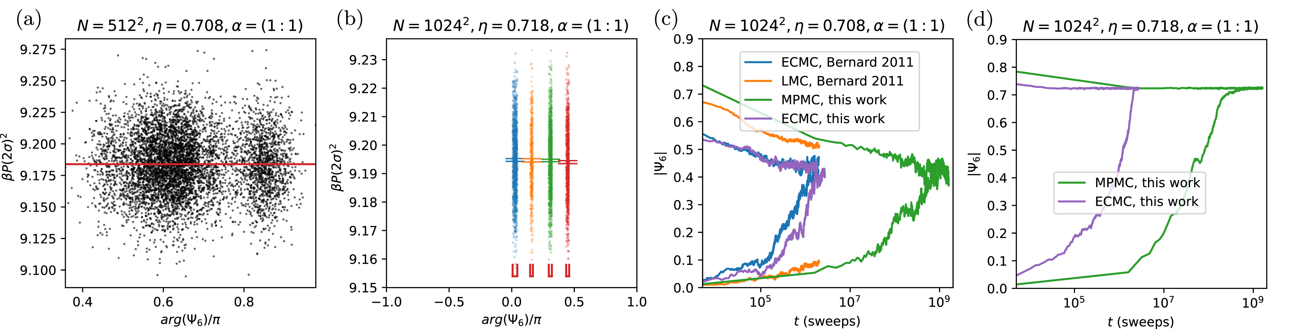
Figure 13: Convergence analysis for the hard-disk model at $\eta=0.708$ and $\eta=0.718$ (square box $\alpha\!=\!(1\!:\!1)$). (a): Scatter plot of the pressure as a function of the orientational order parameter ($N=512^{2}$). (b-d): $N=1024^{2}$ for EDMD and ECMC. (b): Cluster averages obtained from independent runs from initial configurations at specific values of $\Psi_{6}$. The difference, smaller than $10^{-3}$, estimates the systematic error. (c) and (d): Time evolution of the absolute orientational order $|\Psi_{6}|$, starting from either a disordered initial configuration (with $|\Psi_{6}|\gtrsim 0$) or from a crystal (with $|\Psi_{6}|\lesssim 1$) (LMC refers to the local Metropolis algorithm).

$N$	$\alpha$	$P$ / $P_{x},P_{y}$	Method
$64$	$(1\!:\!\sqrt{3}/2)$	$8.065(3),8.137(4)$	Naive
		$8.0671(9),8.1402(9)$	ECMC
$72$	$(9\!:\!4\sqrt{3})$	$8.1614(4),8.2382(5)$	Naive
		$8.1617(7),8.2386(8)$	ECMC
$256^{2}$	$(1\!:\!1)$	$9.172(5)$	ECMC ($g(2\sigma)$)
		$9.1707(2)$	ECMC
		$9.1708(1)$	MPMC
$256^{2}$	$(1\!:\!\sqrt{3}/2)$	$9.176(6)$	ECMC ($g(2\sigma)$)
		$9.1703(2),9.1704(3)$	ECMC
		$9.1704(1),9.1705(1)$	MPMC
$512^{2}$	$(1\!:\!1)$	$9.170(2)$	ECMC ($g(2\sigma)$)
		$9.1699(2)$	ECMC
		$9.1696(1)$	MPMC
$512^{2}$	$(1\!:\!\sqrt{3}/2)$	$9.167(3)$	ECMC ($g(2\sigma)$)
		$9.1694(3),9.1694(3)$	ECMC
		$9.1695(2),9.1697(2)$	MPMC

Table 2: Cross validation of pressure estimates between straight ECMC (naive and state-of-the-art) and MPMC in periodic boxes of given aspect ratio $\alpha$, all at density $\eta=0.698$. MPMC integrates short fictitious runs of straight ECMC, in order to estimate pressures through Eq. (21). ECMC uses the rift-average estimator of Eq. (21), except where indicated to test agreement of the pair-correlation formula of Eq. (27b).

V Conclusion

In this work, we have discussed the hard-disk pressure, which was estimated in the the very first MCMC computation in 1953, and in one of the earliest molecular-dynamics computations, in 1962. We have argued that the difficulty of the pressure estimation had not been fully realized in the decades-long controversy over the phase-transition scenario of this simple model. Our first aim was to provide the context for this computation through a discussion of the physics of the hard-disk model, of the sampling algorithms and pressure estimators and, crucially, of the criteria for bounding mixing times. Our second aim was to finally provide definite high-precision estimates of the pressure through massive computations and to compare them to the values from the literature, thereby ending a long period of uncertainty and doubt. In doing so, we hope to provide benchmarks for the next generation of sampling algorithms, estimators, and physical theories.

The history of the hard-disk model epitomizes a number of prime computational issues. One of them is the role of so-called “computer experiments”, that is, of heuristic simulations which run for much less than the mixing time. The pioneering work of Alder and Wainwright was clearly of that type, as their published pressures explicitly depend on the initial configurations.

Computer experiments below the mixing-time scale are akin to perturbation expansions in the theory of liquids or in quantum mechanics, as the sampling below the mixing-time scale merely “perturbs” around the crystalline or fluid initial configurations. Just like perturbation theory, such computer experiments can provide important insights, yet they have limited predictive power, as was evidenced by the decades-long controversy about the hard-disk phase transitions. Beyond the mixing time, the influence of the initial configuration fades away exponentially, and exponential convergence towards the equilibrium distribution sets in. Only the statistical errors remain. In this regime, MCMC and molecular-dynamics sampling unfolds all its power. Although the mixing and correlation time scales can be gigantic, as discussed, the goal of sampling beyond the mixing time scale must not be lost sight of.

A crucial computational issue for MCMC and molecular-dynamics algorithms consists in estimating the mixing times. We have insisted that simply analyzing a time series (in our case, that of the pressure) is usually not sufficient. Furthermore, we have discussed two strategies to estimate these times reliably for the hard-disk model. First, we designed an observable—the orientational order parameter for hard disks in a square box—with known mean value. We then argued that as long as the run-time average of this observable differed considerably from its known mean, the mixing-time scale has not yet been reached. Used for more than a decade [34, 33], this rotation criterion supposes that the orientational order is the slowest-moving observable in the hard-disk system.

Our second strategy to lend credibility to our MCMC calculations consists in starting from widely different initial configurations, following in the footsteps of Alder and Wainwright, yet accepting the result of the calculation only if the influence of the initial configuration has faded away. This approach is related to the coupling approach for Markov chains [75]. The fluid and crystalline initial configurations that we used to initialize Markov chains for $10^{6}$ disks in the hexatic phase stand in for the worst-case initializations, as they are called for in the definition of the mixing time [47]. The mixing time provides the relevant time scale for analyzing MCMC calculations, and certainly the one where run-time averages become independent of how the Markov chain is initialized.

Finally, we emphasize the role of algorithm development, and of hardware implementations, even in the simple model of hard disks. In this work, we relied heavily on ECMC, which, as evidenced in Fig. 13c and d and d, speeds up MCMC simulations by several orders of magnitude. ECMC is a family of non-reversible Markov chains, rather than a specific algorithm, and variants of the original straight and reflective ECMC continue to be developed. The opportunities granted by non-reversible Markov chains (and by MCMC approaches in general), are certainly very far from having all been explored. The recent extension of ECMC to arbitrary interaction potentials [41] and in particular to the field of molecular simulation [76, 77], carries considerable promise. The spectacular development of GPU hardware over the last fifteen years has greatly democratized parallel computations with, again, one of the cleanest applications being the hard-disk model. Decidedly, this simple model is a “Drosophila” of statistical physics.

Appendix A Extrapolation and statistics

Sampling algorithms output time series of configurations and of pressures (for example one value of the estimated $P_{x}$ for each event chain in $\pm\hat{\mathbf{e}}_{x}$). Further analysis transforms this raw output into the pressure estimates and confidence intervals provided with this work. The pressure estimators that rely on the extrapolation of pair-correlation functions and wall densities have been superseded in recent years by the rift-average estimators. We nevertheless describe them here in order to illustrate that the new estimators are perfectly sound. We also sketch the stationary-bootstrap method which estimates the confidence intervals of the pressure time series.

A.1 Extrapolation of pair correlations and wall densities

The pressure estimator of Eq. (27a) extrapolates the rescaled line densities $\rho_{x}(x)$ and $\rho_{y}(y)$ to $x=\sigma,L_{x}-\sigma$ and $y=\sigma,L_{y}-\sigma$, respectively, and the pair-correlation function $g(r)$ to contact at $r=2\sigma$. We use the fourth-order polynomial histogram fitting procedure of Ref [33] contained in the HistoricDisks software package (see Appendix B). Within our MPMC production runs, however, we use the parameter-free rift-average estimators from fictitious straight-ECMC runs to estimate $P_{x}$ and $P_{y}$, rather than the extrapolation method.

To determine the rescaled line density $\rho_{x}(\sigma)$ (and similarly $\rho_{y}$), the $x$-coordinate of a disk at position $\mathbf{x}_{i}=(x_{i},y_{i})$ is retained in a histogram of bin size $10^{-3}\sigma$ if $x_{i}<1.1\sigma$ or $x_{i}>L_{x}-1.1\sigma$. The histogram is normalized by dividing the number of elements in each bin by $2\times 10^{-3}\sigma nN$, where $n$ is the total number of sampled configurations (not only those contributing to the histogram) and $N$ is the number of disks. The histogram is further multiplied by $L_{x}$ for $\rho_{x}$ (and likewise by $L_{y}$ for $\rho_{y}$) in order to satisfy the normalization $\pi^{(1)}(\mathbf{x}_{i})=\rho(\mathbf{x}_{i})/V$. It is the line density $\rho_{x}(x)$, which is fitted and then extrapolated to $x=\sigma$.

The extrapolation of $g(2\sigma)$ proceeds analogously to that of $\rho_{x}(x)$. The pair distances in the range $2\sigma<r<2.1\sigma$ are retained in a histogram, then normalized by dividing the number of elements in each bin by the bin size $10^{-3}\sigma$ and the total number of sampled distances $nN(N-1)/2$. The normalized histogram approximates $2\pi r\hat{g}(r)$. The histogram is further multiplied by $V/2\pi$ and divided by the distance $r$ corresponding to the center of each bin, yielding the empirical $g(r)$, that is then extrapolated to $r=2\sigma$.

A.2 Statistics

The standard errors in this work were computed with the stationary bootstrap method [78, 79], and double-checked with the blocking method [80]. In stationary bootstrap, the standard error is estimated by creating a large number of simulated time series (typically $1000$). Each of the time series has the same length as the original series, and is created by piecing together randomly chosen sub-series of geometrically distributed length. The only parameter controlling the geometrical distribution is chosen so that it minimizes the mean squared error of the estimated standard error for an infinite sub-series length and for an infinite number of sub-series [81, 82]. The compatibility of the stationary-bootstrap error estimate with that of the blocking method was carefully checked for the entire data presented in the figures as well as in Table 2.

Appendix B Historic data, codes, and validation

The present work is accompanied by the HistoricDisks data and software package, which is published as an open-source project under the GNU GPLv3 license. HistoricDisks is available on GitHub as part of the JeLLyFysh organization . The package provides the pressure data extracted from the literature since $1953$, and also the set of high-precision pressures of the present work (see Subsection B.1). Furthermore, the package contains naive MCMC and MD implementations and pressure estimators (used for validation purposes in Table 1) as well as state-of-the-art implementations used in Section IV.

B.1 Pressure data, equations of states

The pressure data in the HistoricDisks package are from Refs [28, 14, 63, 73, 65, 66, 33, 67], or else correspond to results obtained in this work. Pressure data for a given reference, a given system size and aspect ratio are stored in a separate file in the .csv format (see the README file for details). Pressures and error bars were digitized using the WebPlotDigitizer software [84] where applicable, or else extracted from published tables. The HistoricDisks package furthermore provides Python programs that visualize equations of state. All pressure data are for the $NVT$ ensemble, and the control variable (volume or density, plotted on the $x$-axis) follows all four conventions of Eq. (1). The dependent variable (the pressure, plotted on the $y$-axis) follows two conventions, namely $\beta PV_{0}/N$ and $\beta P(2\sigma)^{2}$. In order to facilitate the direct comparison across different conventions, the produced figures have four $x$-axes and two $y$-axes. The pressure data base in the HistoricDisks package may evolve in the future.

B.2 Computer programs

In addition to pressure data, the HistoricDisks package provides access to sampling algorithms (local Metropolis algorithm, EDMD, and several variants of ECMC). Each algorithm is implemented in two versions. A naive version for four disks in a non-periodic rectangular box is patterned after Ref. [39]. A naive version for $N$ disks in a periodic rectangular box is useful for validation of more advanced methods. Both versions are implemented in Python3 (compatible with PyPy3). In addition, the package provides a state-of-the-art ECMC program for hard disks.

B.2.1 Four-disk non-periodic-box programs

Our naive programs consider four disks of radius $\sigma=0.15$ in a non-periodic square box of sides $1$. We implement the Metropolis algorithm, EDMD, and the straight, reflective [34], forward [54] and Newtonian [55] variants of ECMC. In addition, the pressure estimators of Subsection III.3 are implemented (see Table 1). In detail, we provide pressure estimates from the wall density (using fit of the histogram), from the wall rifts using EDMD, and the wall rifts using ECMC, the latter testing the bias factor $N$ that is introduced because ECMC only moves a single disk. Moreover, we check our rift-average estimators for EDMD and for straight ECMC (that again differ by different biasing factors and mean values of perpendicular velocity components). Finally, we provide a test of the traditional fitting formula involving the pair-correlation function. All these estimators are of thermodynamic origin. As discussed in the main text, the kinematic estimators, including the virial formula, lead to identical formulas and need not be tested independently.

B.2.2 Naive periodic-box programs

The naive periodic-box programs contained in the HistoricDisks package differ from the naive programs only in that the number $N$ of disks and the radius $\sigma$ can be set freely, and that the box is periodic. These programs have some use for demonstration purposes, and to test the more efficient algorithms for relatively small values of $N$. Again, the Metropolis algorithm, EDMD, and the four variants of ECMC are implemented. Run start from crystalline initial configurations. Configurations are output at fixed time intervals. EDMD and straight ECMC also output estimates of the pressure.

B.2.3 State-of-the-art hard-disk programs

The HistoricDisks package contains an optimized C++ code for straight ECMC, that is derived from the Fortran90 code used in [33]. The GPU-based MPMC Cuda code used in this work derives from a general MPMC code for soft-sphere models and will be published elsewhere [85]. Pressures obtained from these implementations agree within very tight error bars (see Table 2). A Python script contained in the package analyzes samples that were saved from these two codes in the HDF5 [86] file format. It computes for example the global orientational order parameters $\Psi_{6}$.

References

- Kapitza [1938] P. Kapitza, Viscosity of Liquid Helium below the -Point, Nature 141, 74 (1938).
- Vaks and Larkin [1966] V. G. Vaks and A. I. Larkin, On phase transitions of second order, J. Exp. Theor. Phys. 22, 678 (1966).
- Campostrini et al. [2006] M. Campostrini, M. Hasenbusch, A. Pelissetto, and E. Vicari, Theoretical estimates of the critical exponents of the superfluid transition in by lattice methods, Phys. Rev. B 74, 144506 (2006).
- Hasenbusch [2019] M. Hasenbusch, Monte Carlo study of an improved clock model in three dimensions, Phys. Rev. B 100, 224517 (2019).
- Chester et al. [2020] S. M. Chester, W. Landry, J.Liu, D. Poland, D. Simmons-Duffin, N. Su, and A. Vichi, Carving out OPE space and precise O(2) model critical exponents, J. High Energy Phys. 2020 (6).
- Pollock and Ceperley [1987] E. L. Pollock and D. M. Ceperley, Path-integral computation of superfluid densities, Phys. Rev. B 36, 8343 (1987).
- Wilson [1983] K. G. Wilson, The renormalization group and critical phenomena, Rev. Mod. Phys. 55, 583 (1983).
- Lipa et al. [1996] J. A. Lipa, D. R. Swanson, J. A. Nissen, T. C. P. Chui, and U. E. Israelsson, Heat Capacity and Thermal Relaxation of Bulk Helium very near the Lambda Point, Phys. Rev. Lett. 76, 944 (1996).
- Lipa et al. [2003] J. A. Lipa, J. A. Nissen, D. A. Stricker, D. R. Swanson, and T. C. P. Chui, Specific heat of liquid helium in zero gravity very near the lambda point, Phys. Rev. B 68, 10.1103/physrevb.68.174518 (2003).
- Muller [1946] H. J. Muller, Nobel Lecture: The Production of Mutations (1946).
- Nüsslein-Volhard [1995] C. Nüsslein-Volhard, Nobel Lecture: The Identification of Genes Controlling Development in Flies and Fishes (1995).
- Kohler [1994] R. E. Kohler, Lords of the Fly: Drosophila Genetics and the Experimental Life, History, philosophy, and social studies of science : Biology (University of Chicago Press, 1994).
- Dietrich et al. [2014] M. R. Dietrich, R. A. Ankeny, and P. M. Chen, Publication Trends in Model Organism Research, Genetics 198, 787 (2014).
- Alder and Wainwright [1962] B. J. Alder and T. E. Wainwright, Phase Transition in Elastic Disks, Phys. Rev. 127, 359 (1962).
- Kosterlitz and Thouless [1973] J. M. Kosterlitz and D. J. Thouless, Ordering, metastability and phase transitions in two-dimensional systems, J. Phys. C: Solid State Phys. 6, 1181 (1973).
- Bernoulli [1738] D. Bernoulli, Hydrodynamica (1738).
- Sinai [1970] Y. G. Sinai, Dynamical systems with elastic reflections, Russ. Math. Surv. 25, 137 (1970).
- Simányi [2003] N. Simányi, Proof of the Boltzmann-Sinai ergodic hypothesis for typical hard disk systems, Invent. Math. 154, 123 (2003).
- Lebowitz and Penrose [1964] J. L. Lebowitz and O. Penrose, Convergence of Virial Expansions, J. Math. Phys. 5, 841 (1964).
- Helmuth et al. [2022] T. Helmuth, W. Perkins, and S. Petti, Correlation decay for hard spheres via Markov chains, Ann. Appl. Probab. 32, 10.1214/21-aap1728 (2022).
- Boltzmann [1995] L. Boltzmann, Lectures on Gas Theory, Dover Books on Physics (Dover Publications, 1995).
- Fejes [1940] L. Fejes, Über einen geometrischen Satz, Math. Z. 46, 83 (1940).
- Richthammer [2007] T. Richthammer, Translation-Invariance of Two-Dimensional Gibbsian Point Processes, Commun. Math. Phys. 274, 81 (2007).
- Richthammer [2016] T. Richthammer, Lower Bound on the Mean Square Displacement of Particles in the Hard Disk Model, Commun. Math. Phys. 345, 1077 (2016).
- Kirkwood and Monroe [1941] J. G. Kirkwood and E. Monroe, Statistical Mechanics of Fusion, J. Chem. Phys. 9, 514 (1941).
- Battimelli and Ciccotti [2018] G. Battimelli and G. Ciccotti, Berni Alder and the pioneering times of molecular simulation, Eur. Phys. J. H 43, 303 (2018).
- Peierls [1935] R. Peierls, Quelques propriétés typiques des corps solides, Annales de l’I. H. P. 5, 177 (1935).
- Metropolis et al. [1953] N. Metropolis, A. W. Rosenbluth, M. N. Rosenbluth, A. H. Teller, and E. Teller, Equation of State Calculations by Fast Computing Machines, J. Chem. Phys. 21, 1087 (1953).
- Mayer and Wood [1965] J. E. Mayer and W. W. Wood, Interfacial Tension Effects in Finite, Periodic, Two-Dimensional Systems, J. Chem. Phys. 42, 4268 (1965).
- Kosterlitz [1974] J. M. Kosterlitz, The critical properties of the two-dimensional xy model, J. Phys. C: Solid State Phys. 7, 1046 (1974).
- Halperin and Nelson [1978] B. I. Halperin and D. R. Nelson, Theory of Two-Dimensional Melting, Phys. Rev. Lett. 41, 121 (1978).
- Young [1979] A. P. Young, Melting and the vector Coulomb gas in two dimensions, Phys. Rev. B 19, 1855 (1979).
- Bernard and Krauth [2011] E. P. Bernard and W. Krauth, Two-Step Melting in Two Dimensions: First-Order Liquid-Hexatic Transition, Phys. Rev. Lett. 107, 155704 (2011).
- Bernard et al. [2009] E. P. Bernard, W. Krauth, and D. B. Wilson, Event-chain Monte Carlo algorithms for hard-sphere systems, Phys. Rev. E 80, 056704 (2009).
- Lee and Strandburg [1992] J. Lee and K. J. Strandburg, First-order melting transition of the hard-disk system, Phys. Rev. B 46, 11190 (1992).
- Andersen [1980] H. C. Andersen, Molecular dynamics simulations at constant pressure and/or temperature, J. Chem. Phys. 72, 2384 (1980), https://doi.org/10.1063/1.439486 .
- Parrinello and Rahman [1981] M. Parrinello and A. Rahman, Polymorphic transitions in single crystals: A new molecular dynamics method, J. Appl. Phys. 52, 7182 (1981), https://doi.org/10.1063/1.328693 .
- Rowley et al. [1975] L. A. Rowley, D. Nicholson, and N. G. Parsonage, Monte Carlo grand canonical ensemble calculation in a gas-liquid transition region for 12-6 Argon, J. Comput. Phys. 17, 401 (1975).
- Krauth [2006] W. Krauth, Statistical Mechanics: Algorithms and Computations (Oxford University Press, 2006).
- Asakura and Oosawa [1954] S. Asakura and F. Oosawa, On Interaction between Two Bodies Immersed in a Solution of Macromolecules, J. Chem. Phys. 22, 1255 (1954).
- Michel et al. [2014] M. Michel, S. C. Kapfer, and W. Krauth, Generalized event-chain Monte Carlo: Constructing rejection-free global-balance algorithms from infinitesimal steps, J. Chem. Phys. 140, 054116 (2014).
- Alder and Wainwright [1957] B. J. Alder and T. E. Wainwright, Phase Transition for a Hard Sphere System, J. Chem. Phys. 27, 1208 (1957).
- Rapaport [1980] D. C. Rapaport, The Event Scheduling Problem in Molecular Dynamic Simulation, J. Comput. Phys. 34, 184 (1980).
- Rapaport [2009] D. C. Rapaport, The Event-Driven Approach to N-Body Simulation, Prog. Theor. Exp. Phys. 178, 5 (2009), https://academic.oup.com/ptps/article-pdf/doi/10.1143/PTPS.178.5/5288894/178-5.pdf .
- Bannerman et al. [2011] M. N. Bannerman, R. Sargant, and L. Lue, DynamO: a free general event-driven molecular dynamics simulator, J. Comput. Chem. 32, 3329 (2011).
- Lubachevsky [1992] B. D. Lubachevsky, Simulating billiards: Serially and in parallel, International Journal in Computer Simulation 2, 373 (1992).
- Levin et al. [2008] D. A. Levin, Y. Peres, and E. L. Wilmer, Markov Chains and Mixing Times (American Mathematical Society, 2008).
- Anderson et al. [2013] J. A. Anderson, E. Jankowski, T. L. Grubb, M. Engel, and S. C. Glotzer, Massively parallel Monte Carlo for many-particle simulations on GPUs, J. Comput. Phys. 254, 27 (2013).
- Engel et al. [2013] M. Engel, J. A. Anderson, S. C. Glotzer, M. Isobe, E. P. Bernard, and W. Krauth, Hard-disk equation of state: First-order liquid-hexatic transition in two dimensions with three simulation methods, Phys. Rev. E 87, 042134 (2013).
- Chen et al. [1999] F. Chen, L. Lovász, and I. Pak, Lifting Markov Chains to Speed up Mixing, Proceedings of the 17th Annual ACM Symposium on Theory of Computing , 275 (1999).
- Diaconis et al. [2000] P. Diaconis, S. Holmes, and R. M. Neal, Analysis of a nonreversible Markov chain sampler, Ann. Appl. Probab. 10, 726 (2000).
- Krauth [2021] W. Krauth, Event-Chain Monte Carlo: Foundations, Applications, and Prospects, Front. Phys. 9, 229 (2021).
- Höllmer et al. [2022] P. Höllmer, N. Noirault, B. Li, A. C. Maggs, and W. Krauth, Sparse Hard-Disk Packings and Local Markov Chains, J. Stat. Phys. 187, 10.1007/s10955-022-02908-4 (2022).
- Michel et al. [2020] M. Michel, A. Durmus, and S. Sénécal, Forward Event-Chain Monte Carlo: Fast Sampling by Randomness Control in Irreversible Markov Chains, J. Comput. Graph. Stat. 29, 689 (2020).
- Klement and Engel [2019] M. Klement and M. Engel, Efficient equilibration of hard spheres with Newtonian event chains, J. Chem. Phys. 150, 174108 (2019).
- Li et al. [2021] B. Li, S. Todo, A. C. Maggs, and W. Krauth, Multithreaded event-chain Monte Carlo with local times, Comput. Phys. Commun. 261, 107702 (2021).
- Li et al. [2022] B. Li, Y. Nishikawa, A. C. Maggs, and W. Krauth, Multithreaded event-chain Monte Carlo: Implementation and benchmarks, Manuscript in preparation (2022).
- Qin et al. [2022] L. Qin, P. Höllmer, and W. Krauth, Direction-sweep markov chains, J. Phys. A: Math. Theor. 55, 105003 (2022).
- Eppenga and Frenkel [1984] R. Eppenga and D. Frenkel, Monte Carlo study of the isotropic and nematic phases of infinitely thin hard platelets, Mol. Phys. 52, 1303 (1984).
- Brumby et al. [2011] P. E. Brumby, A. J. Haslam, E. de Miguel, and G. Jackson, Subtleties in the calculation of the pressure and pressure tensor of anisotropic particles from volume-perturbation methods and the apparent asymmetry of the compressive and expansive contributions, Mol. Phys. 109, 169 (2011).
- de Miguel and Jackson [2006] E. de Miguel and G. Jackson, The nature of the calculation of the pressure in molecular simulations of continuous models from volume perturbations, J. Chem. Phys. 125, 164109 (2006), https://doi.org/10.1063/1.2363381 .
- Allen [2006] M. P. Allen, Evaluation of pressure tensor in constant-volume simulations of hard and soft convex bodies, J. Chem. Phys. 124, 214103 (2006), https://doi.org/10.1063/1.2202352 .
- Zollweg and Chester [1992] J. A. Zollweg and G. V. Chester, Melting in two dimensions, Phys. Rev. B 46, 11186 (1992).
- Jaster [1999a] A. Jaster, Computer simulations of the two-dimensional melting transition using hard disks, Phys. Rev. E 59, 2594 (1999a).
- Jaster [2004] A. Jaster, The hexatic phase of the two-dimensional hard disk system, Phys. Lett. A 330, 120 (2004).
- Mak [2006] C. H. Mak, Large-scale simulations of the two-dimensional melting of hard disks, Phys. Rev. E 73, 065104 (2006).
- Qi et al. [2014] W. Qi, A. P. Gantapara, and M. Dijkstra, Two-stage melting induced by dislocations and grain boundaries in monolayers of hard spheres, Soft Matter 10, 5449 (2014).
- Weber et al. [1995] H. Weber, D. Marx, and K. Binder, Melting transition in two dimensions: A finite-size scaling analysis of bond-orientational order in hard disks, Phys. Rev. B 51, 14636 (1995).
- Mitus et al. [1997] A. C. Mitus, H. Weber, and D. Marx, Local structure analysis of the hard-disk fluid near melting, Phys. Rev. E 55, 6855 (1997).
- Binder et al. [2002] K. Binder, S. Sengupta, and P. Nielaba, The liquid-solid transition of hard discs: first-order transition or Kosterlitz-Thouless-Halperin-Nelson-Young scenario?, J. Phys. Condens. Matter 14, 2323 (2002).
- Kannan et al. [2003] R. Kannan, M. W. Mahoney, and R. Montenegro, Rapid mixing of several Markov chains for a hard-core model, in Proc. 14th annual ISAAC, Lecture Notes in Computer Science (Springer, Berlin, Heidelberg, 2003) pp. 663–675.
- Note [1] In our simulations, we confirm that the orientational order parameter has been rotated more than ° and has visited at least one of the two points on the real axis, , and one on the imaginary axis, .
- Jaster [1999b] A. Jaster, An improved Metropolis algorithm for hard core systems, Physica A 264, 134 (1999b).
- Lubachevsky and Stillinger [1990] B. D. Lubachevsky and F. H. Stillinger, Geometric properties of random disk packings, J. Stat. Phys. 60, 561 (1990).
- Propp and Wilson [1996] J. G. Propp and D. B. Wilson, Exact sampling with coupled Markov chains and applications to statistical mechanics, Random Struct Alg. 9, 223 (1996).
- Faulkner et al. [2018] M. F. Faulkner, L. Qin, A. C. Maggs, and W. Krauth, All-atom computations with irreversible Markov chains, J. Chem. Phys. 149, 064113 (2018).
- Höllmer et al. [2020] P. Höllmer, L. Qin, M. F. Faulkner, A. Maggs, and W. Krauth, JeLLyFysh-Version1.0 — a Python application for all-atom event-chain Monte Carlo, Comput. Phys. Commun. 253, 107168 (2020).
- Politis and Romano [1994] D. N. Politis and J. P. Romano, The Stationary Bootstrap, J. Am. Stat. Assoc. 89, 1303 (1994).
- Nishikawa et al. [2021] Y. Nishikawa, J. Takahashi, and T. Takahashi, Stationary Bootstrap: A Refined Error Estimation for Equilibrium Time Series (2021), 2112.11837 .
- Flyvbjerg and Petersen [1989] H. Flyvbjerg and H. G. Petersen, Error estimates on averages of correlated data, J. Chem. Phys. 91, 461 (1989).
- Politis and White [2004] D. N. Politis and H. White, Automatic Block-Length Selection for the Dependent Bootstrap, Econom. Rev. 23, 53 (2004).
- Patton et al. [2009] A. Patton, D. N. Politis, and H. White, Correction to “Automatic Block-Length Selection for the Dependent Bootstrap” by D. Politis and H. White, Econom. Rev. 28, 372 (2009).
- Note [2] The url of the repository is https://github.com/jellyfysh/HistoricDisks.
- Rohatgi [2021] A. Rohatgi, Webplotdigitizer: Version 4.5 (2021).
- Nishikawa et al. [2022] Y. Nishikawa, W. Krauth, and A. C. Maggs, Two-dimensional soft spheres - phase diagrams and phase transitions, Manuscript in preparation (2022).
- The HDF Group [2022] The HDF Group, Hierarchical Data Format, version 5 (1997-2022).