Support Vector Machines with the Hard-Margin Loss: Optimal Training via Combinatorial Benders’ Cuts

Abstract. The classical hinge-loss support vector machines (SVMs) model is sensitive to outlier observations due to the unboundedness of its loss function. To circumvent this issue, recent studies have focused on non-convex loss functions, such as the hard-margin loss, which associates a constant penalty to any misclassified or within-margin sample. Applying this loss function yields much-needed robustness for critical applications but it also leads to an NP-hard model that makes training difficult, since current exact optimization algorithms show limited scalability, whereas heuristics are not able to find high-quality solutions consistently. Against this background, we propose new integer programming strategies that significantly improve our ability to train the hard-margin SVM model to global optimality. We introduce an iterative sampling and decomposition approach, in which smaller subproblems are used to separate combinatorial Benders’ cuts. Those cuts, used within a branch-and-cut algorithm, permit to converge much more quickly towards a global optimum. Through extensive numerical analyses on classical benchmark data sets, our solution algorithm solves, for the first time, 117 new data sets to optimality and achieves a reduction of 50% in the average optimality gap for the hardest datasets of the benchmark.

Keywords. Support vector machines, Hard margin loss, Branch-and-cut, Combinatorial Benders’ cuts, Sampling strategies

^∗ Correspondence to: isantana@inf.puc-rio.br, thibaut.vidal@cirrelt.ca

1 Introduction

Support vector machines (SVMs) are among the most popular classification models due to their simplicity and solid theoretical foundations from statistical learning [34, 47, 54]. Application fields of SVMs include, among others, image classification, bioinformatics, handwritten digits recognition, face detection, and generalized predictive control [6, 9, 16]. Beyond this, SVMs are regularly used as elementary building blocks of sophisticated AutoML pipelines [21]. They achieve state-of-the-art results for a variety of applications, especially for large-scale datasets [10, 13, 30].

In its simplest form, an SVM can be defined as follows. Let $(\mathbf{X},\mathbf{y})=\{\mathbf{x}_{i},y_{i}\}$ be a training set in which each $\mathbf{x}_{i}\in\mathbb{R}^{m}$ is an $m$-dimensional feature vector, and each $y_{i}\in\{-1,1\}$ is its associated class. Then, an SVM seeks a hyperplane $\mathcal{H}=\{\mathbf{x}\in\mathbb{R}^{m}:\mathbf{w}\cdot\mathbf{x}+b=0\}$ that optimizes the following objective:

$$\min\limits_{\mathbf{w},b}\frac{1}{2}||\mathbf{w}||^{2}+C\sum_{i=1}^{n}f(y_{i}(\mathbf{w}\cdot\mathbf{x}_{i}+b)).$$ (1)

The first term of Equation (1) acts as a regularization term and indirectly maximizes the margin of the SVM [47], whereas the second term ensures fidelity to the data and penalizes misclassified samples, with coefficient $C$ balancing the two terms. Accordingly, the objective establishes a trade-off between maximizing the hyperplane’s margin and minimizing the concomitant misclassification error. The loss function $f$ varies with respect to the studied problem variant. In the classical SVM with hinge loss (SVM-HL), we define

$$f(u):=f_{\textsc{Hinge}}(u)=\max\{0,1-u\},$$ (2)

such that a misclassified sample, i.e., a sample for which $y_{i}(\mathbf{w}\cdot\mathbf{x}_{i}+b)<1$, directly increases the objective value of Equation (1) proportionally to its error (see Figure 2).

However, while the classical convex SVM-HL permits fast training and scalability, it is also known to lack robustness in the presence of misclassified samples or outliers since its loss function is unbounded. As a drawback, the trained model can be severely affected by these outliers, preventing its application in several domains, especially for high-stakes decisions where robustness is critical [42].

In light of this, some works have considered the use of bounded but non-convex loss functions in an attempt to gain robustness [see, e.g., 5, 29, 53]. In particular, the SVM with hard-margin loss (SVM-HML) uses

$$f(u):=f_{\textsc{Hard}}(u)=\begin{cases}1&\text{ if }u<1\\ 0&\text{ otherwise,}\end{cases}$$ (3)

such that any misclassified sample (or sample within the margin) leads to a unit penalty (see Figure 2), therefore limiting the influence of misclassified samples on $\mathcal{H}$ and increasing classification robustness.

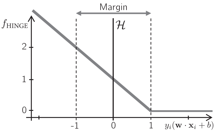
Figure 1: Hinge loss function

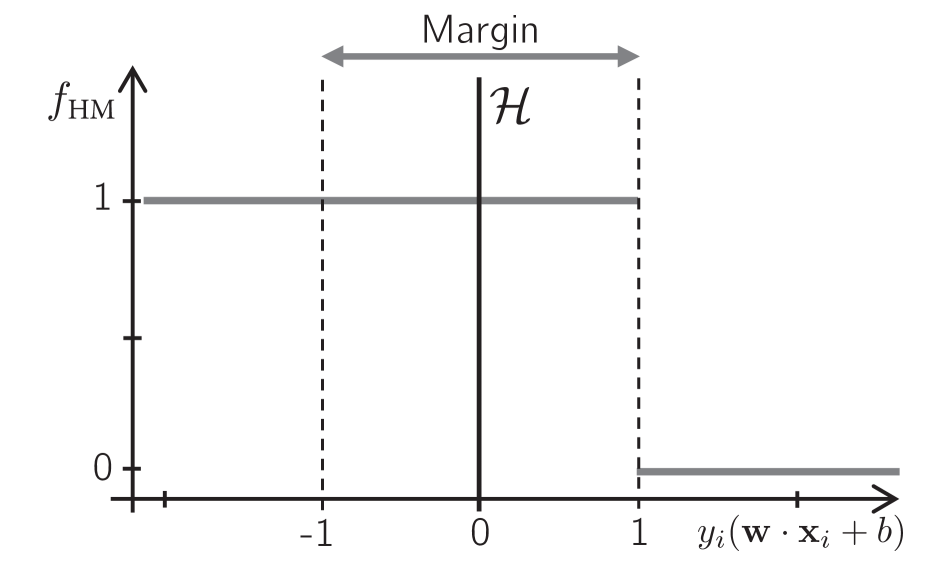
Figure 2: Hard-margin loss function

However, this much-needed robustness comes at the expense of computational efficiency since training SVM-HML requires solving a mixed-integer quadratic problem (MIQP) and is NP-hard [11]. This hardness, but more especially the inability to efficiently solve the SVM-HML, limits its current use. Training SVM-HML models to global optimality is currently only achievable for very small datasets, whereas current heuristics for training do not consistently find high-quality hyperplanes.

In this work, we contribute towards addressing those challenges and pave the way toward more efficient global optimization algorithms. We propose new mixed-integer programming approaches to train SVM-HML models to global optimality. We exploit the problem’s structure to devise efficient decomposition techniques, relying on subsets of the samples to generate Combinatorial Benders’ (CB) cuts quickly. More specifically, the contribution of this paper is fourfold:

• We show that CB cuts can be successfully exploited to generate useful inequalities for SVM-HML.

• We introduce sampling strategies that permit to quickly generate a diversified pool of cuts. We effectively embed these cuts within a branch-and-cut algorithm, leading to an efficient training algorithm that can achieve global optimality.

• We conduct an extensive numerical campaign to measure the performance of our training approach and the impact of important design choices. As seen in our experiments, this algorithm significantly improves the current status-quo regarding the solution of SVM-HML, solving for the first time 117 new data sets to optimality and achieving a reduction of 50% in the average optimality gap over previous approaches for the hardest datasets of the benchmark.

• Generally, our study underlines the benefits of applying cutting-edge mixed-integer programming techniques to combinatorial optimization problems that arise when training non-convex machine learning models.

The remainder of this paper is organized as follows. Section 2 briefly reviews the related literature. Section 3 introduces the proposed methodology. Section 4 details our computational experiments, and Section 5 concludes this paper.

2 Related Literature

A vast body of literature on SVMs exists, covering various topics such as applications, training algorithms, and loss functions. For the sake of brevity, we focus on recent contributions to training algorithms for SVM-HL as well as works on SVMs with non-convex loss functions, namely SVM-HML and the SVM with ramp loss (SVM-RL).

The training problem for the classical SVM-HL can be cast and efficiently solved as a continuous convex quadratic programming problem. Existing solution approaches typically detect and fix violations of first-order optimality conditions, leading to a series of small subproblems with few variables. A classical approach, called Sequential Minimal Optimization (SMO) is used in several state-of-the-art implementations [10, 13, 30, 40] and consists of solving a restricted problem of only two variables at each iteration. Still, some algorithms have also exploited larger subproblems [see, e.g., 20, 30, 48]. Training algorithms for SVM-HL are quite diverse and base on data-selection concepts [32, 33], geometric methods [34] and heuristics [51]. For a detailed presentation of algorithms for the SVM-HL and its variants, we refer the reader to the surveys of Carrizosa and Morales [8], Cervantes et al. [9], and Wang et al. [50], as well as to the book of Schölkopf et al. [43].

Despite its widespread use, the sensitivity of SVM-HL to outliers has regularly raised obstacles when dealing with critical applications. Consequently, a part of recent research has explored the possibility of using non-convex loss functions to gain robustness. Brooks [5] focused on two non-convex loss functions in particular: the SVM-HML [36, 37, 39] and the SVM-RL [14, 45, 46]. Both of these functions are bounded, such that the contribution of each sample to the objective is limited. In the SVM-RL model, any sample within the margin receives a linear penalty proportional to its distance to the margin (a value between $0$ and $2C$), whereas any misclassified sample outside the margin receives a fixed penalty of $2C$. In the SVM-HML, the penalty of any misclassified or within-margin sample is simply fixed to a constant $C$.

The solution algorithm proposed by Brooks [5] solves the training problem as a mixed-integer quadratic programming (MIQP) using state-of-the-art branch-and-cut solvers. For the SVM-HML and SVM-RL, the authors rely on indicator constraints representing logical implications between a binary variable representing the status of each sample (misclassified or not) and a linear constraint that evaluates its relative position from the separating hyperplane. However, it is well known that such constraints can be reformulated in linear form using a “big-M” constant, but doing so without carefully tuning the value of the M constant typically leads to an ineffective formulation with a weak linear relaxation, impeding an efficient solution by branch-and-cut [52].

For the SVM-RL setting, Huang et al. [29] explored the ramp loss function with $\ell_{1}$-penalty, resulting in a piecewise linear programming problem. Later, Belotti et al. [3] compared different formulations for the logical constraints and concluded that aggressive bound-tightening techniques are necessary for a successful solution approach. The strategy derived from their studies has been since implemented as a standard routine for handling such constraints in the commercial solver CPLEX for MILP/MIQPs. Finally, Baldomero-Naranjo et al. [2] tightened the M constants by solving sequences of continuous problems and Lagrangian relaxations. For the SVM-HML, Poursaeidi and Kundakcioglu [41] proposed hard-margin loss formulations within the context of multiple-instances classification, a setting in which class labels are defined as sets. Finally, in [28], the hard-margin loss was transformed into a re-scaled hinge loss function for imbalanced noisy classification.

Concluding, only a few studies have attempted to improve the state-of-the-art training algorithms for SVM-HML after the seminal work of Brooks [5], often by concentrating on the handling of the logical constraints and the proper calibration of the $M$ constants. Despite this progress, optimal training remains limited to data sets counting a few hundred samples. To improve this status-quo, we investigate a different approach, which consists of the separation of CB cuts and their combination with classical logical constraints to achieve a valid problem formulation with a better linear relaxation. Moreover, to improve computational efficiency, we rely on sampling techniques for a fast generation of diverse cuts.

3 Methodology

We first recall the classical mathematical programming formulations for the SVM variants that are of interest for our study, namely SVM-HL and SVM-HML, and then proceed with a description of our algorithmic approach.

3.1 Descriptive formulations

The SVM with hinge loss (also known as soft-margin SVM) associates to misclassified and within-margin samples a penalty that is proportional to their distance in relation to the “correctly classified margin” of the found hyperplane (see Figure 2).

Let $\mathbf{w}\in\mathbb{R}^{m}$ be a vector of real variables that represents the coordinates of the hyperplane, let $b$ be its intercept to the origin, and let $\xi_{i}$ represent the misclassification penalty of sample $i$. With these notations, the training problem for SVM-HL can be mathematically formulated as:

$$\min\limits_{\mathbf{w},b,\xi}\hskip 8.5359pt \frac{1}{2}||\mathbf{w}||^{2}+C\sum_{i=1}^{n}\xi_{i}$$ (4)

s.t. $$y_{i}(\mathbf{w}\cdot\mathbf{x}_{i}+b)\geq 1-\xi_{i},\quad i\in\{1,\dots,n\}$$ (5)

$$\xi_{i}\geq 0,\quad i\in\{1,\dots,n\}.$$ (6)

Objective (4) seeks a maximum margin separator through the term $\frac{1}{2}||\mathbf{w}||^{2}$ and minimizes the total misclassification penalty $C\sum_{i=1}^{n}\xi_{i}$, where $C>0$ is a constant that balances both parts of the objective. Moreover, Constraints (5) calculate the misclassification penalty of each sample.

In the SVM with hard-margin loss, misclassified samples are associated a fixed penalty cost. Binary variables $z$ are used to indicate whether a sample $i$ is misclassified or within the margin ($z_{i}=1$), or correctly classified ($z_{i}=0$). The SVM-HML can be formulated as follows:

$$\min\limits_{\mathbf{w},b,z}\hskip 8.5359pt \frac{1}{2}||\mathbf{w}||^{2}+C\sum_{i=1}^{n}z_{i}$$ (7)

s.t. $$(z_{i}=0)\Rightarrow y_{i}(\mathbf{w}\cdot\mathbf{x}_{i}+b)\geq 1 i\in\{1,\dots,n\}$$ (8)

$$z_{i}\in\{0,1\} i\in\{1,\dots,n\}.$$ (9)

In this formulation, the penalty term in the objective (7) is directly proportional to the number of misclassified samples. Constraints (8), represented as logical constraints, ensure that $z_{i}=0$ only if sample $i$ is correctly classified. These constraints are strictly speaking not part of the semantic of a MILP/MIQP, but they could be directly transformed into a linear constraint by using a big-M constant and imposing $y_{i}(\mathbf{w}\cdot\mathbf{x}_{i}+b)\geq 1-Mz_{i}$. The drawback of such a reformulation is that it leads to a formulation that provides notably weaker linear-relaxation bounds, rendering branch-and-bound algorithms relatively inefficient.

3.2 Combinatorial Benders’ cuts

To optimally solve the SVM-HML, we propose a solution method based on Benders’ decomposition [4]. In its canonical form, this strategy exploits the structure of a mixed-integer linear program and splits its variables into two subsets. The first subset of integer or continuous variables (sometimes called “complicating variables”) is selected in such a way that fixing them either decomposes or reduces the complexity of the resulting problem. The remaining variables should be continuous. The method then works by decomposing the original problem into a master problem (MP), solved over the complicating variables, and a subproblem (SP), solved as a linear program over the remaining continuous variables. The algorithm iteratively produces an incumbent solution of the MP and uses the dual of the SP to assess its feasibility. If the SP determines that the incumbent solution is feasible, then this information is integrated into the MP in the form of an additional CB cut, which eliminates the infeasible incumbent solution.

The studies of Hooker and Ottosson [27] and Codato and Fischetti [12] paved the way towards efficient applications of Benders’ decomposition to a broad class of mixed-integer programming problems (MIPs) with logical constraints. Notably, the so-called CB approach leads among others to a new solution paradigm for models of the following form:

$$\min\hskip 8.5359pt \mathbf{c}^{\intercal}\mathbf{z}$$ (10)

s.t. $$(z_{i}=0)\Rightarrow\mathbf{a_{i}}^{\intercal}\,\mathbf{y}\geq d_{i} i\in\{1,\dots,n\}$$ (11)

$$\mathbf{z}\in\{0,1\}^{n}$$ (12)

$$\mathbf{y}\in Y,$$ (13)

with binary complicating variables $\mathbf{z}$, continuous variables $\mathbf{y}$ in a polytope $Y$ (i.e., respecting a set of linear inequalities), and linear weights $\mathbf{c}$ (applied only on the coefficients of $\mathbf{z}$) to calculate the objective. In a CB approach, Model (10–13) is reformulated as follows:

$$\min\hskip 8.5359pt \mathbf{c}^{\intercal}\mathbf{z}$$ (14)

s.t. $$\sum_{i\in S}z_{i}\geq 1 S\in\mathcal{S}^{\textsc{mis}}$$ (15)

$$\mathbf{z}\in\{0,1\}^{n},$$ (16)

where $\mathcal{S}^{\textsc{mis}}$ is the collection of all inclusion-minimal infeasible subsystems (MIS) of rows:

$$\mathcal{S}^{\textsc{mis}}=\left\{S\ \left\lvert\ \begin{aligned} &\{\mathbf{a_{i}}^{\intercal}\,\mathbf{y}\geq d_{i}\ \forall i\in S,\mathbf{y}\in Y\}\text{ is infeasible}\\ &\{\mathbf{a_{i}}^{\intercal}\,\mathbf{y}\geq d_{i}\ \forall i\in\hat{S},\mathbf{y}\in Y\}\text{ is feasible}\ \forall\hat{S}\subset S\end{aligned}\right.\right\}.\\$$ (17)

Notably, this formulation no longer contains logical implications or big-M terms. However, it includes an exponential number of constraints. For this reason, the CB approach consists of dynamically detecting and adding Constraints (15). As in a classical Benders’ decomposition, the method alternates between solving the master problem with only a subset of the constraints $\mathcal{S}\subset\mathcal{S}^{\textsc{mis}}$ found so far, and solving a subproblem to identify new violated constraints that cut the incumbent solution of the master in case of infeasibility. Finally, we observe that $\mathcal{S}^{\textsc{mis}}$ does not need to be restricted to “inclusion-minimal” subsets of rows to yield a valid formulation, but doing so significantly reduces the number of constraints in the set.

Despite its successful application in a variety of settings [1, 15, 19], the aforementioned CB framework is not directly applicable to problems with objective functions that contain both complicating variables $\mathbf{z}$ and continuous variables $\mathbf{y}$. This is unfortunately the case for the SVM-HML, due to the occurrence of the continuous variables $\mathbf{w}$ and $b$ in the objective and the logical implications. To circumvent this issue, we introduce a weaker set of CB cuts in conjunction with the original logical implication constraints to design an effective solution method. In this case, the cuts do not carry the burden of ensuring the model’s validity, but nevertheless contribute to strengthening the formulation to obtain a better linear relaxation and improve the solution process.

3.3 Combinatorial Benders’ cuts and the SVM-HML

We first start by describing a direct application of CB to the SVM-HML and by analyzing its shortcomings. This would lead to the following formulation:

$$\min\limits_{W,\mathbf{z}}\hskip 8.5359pt \frac{1}{2}W^{2}+C\sum_{i=1}^{n}z_{i}$$ (18)

s.t. $$\sum_{i\in S}z_{i}\geq 1\hskip 227.62204ptS\in\mathcal{S}_{\textsc{svm-hml}}^{\textsc{mis}}(W)$$ (19)

$$\mathbf{z}\in\{0,1\}^{n}$$ (20)

with $$\mathcal{S}_{\textsc{svm-hml}}^{\textsc{mis}}(W)=\left\{S\ \left\lvert\ \begin{aligned} &\{y_{i}(\mathbf{w}\cdot\mathbf{x}_{i}+b)\geq 1\ \forall i\in S,\ ||w||^{2}\leq W^{2}\}\text{ is infeasible}\\ &\{y_{i}(\mathbf{w}\cdot\mathbf{x}_{i}+b)\geq 1\ \forall i\in\hat{S},\ ||w||^{2}\leq W^{2}\}\text{ is feasible}\ \forall\hat{S}\subset S\end{aligned}\right.\right\}.$$ (21)

As seen in this formulation, $W$ appears in the objective and also characterizes the set of Benders’ cuts. Unfortunately, the resulting formulation can no longer be practically solved as a MILP or MIQP due to this dependency. To remedy this issue, we leverage Property 1.

Property 1.

Let $W_{\textsc{ub}}$ be a valid upper bound on $W$ on any optimal solution of Problem (18–21). Then, $\mathcal{S}_{\textsc{svm-hml}}^{\textsc{mis}}(W_{\textsc{ub}})$ is also set of valid inequalities for the SVM-HML.

Proof. Consider $S\in\mathcal{S}_{\textsc{svm-hml}}^{\textsc{mis}}(W_{\textsc{ub}})$. Due to the definition of $\mathcal{S}_{\textsc{svm-hml}}^{\textsc{mis}}(W_{\textsc{ub}})$, $\{y_{i}(\mathbf{w}\cdot\mathbf{x}_{i}+b)\geq 1\ \forall i\in S$ with $||w||^{2}\leq W_{\textsc{ub}}^{2}\}$ is an infeasible subsystem. Given that all optimal solutions of Problem (18–21) satisfy $W\leq W_{\textsc{ub}}$, then $\{y_{i}(\mathbf{w}\cdot\mathbf{x}_{i}+b)\geq 1\ \forall i\in S$ with $||w||^{2}\leq W^{2}\}$ is also an infeasible subsystem, and therefore at least one sample $i$ in $S$ must be misclassified, implying that $\sum_{i\in S}z_{i}\geq 1$ is a valid inequality.

With this property, the dependence upon parameter $W$ can be avoided as soon as a valid upper bound is known. The quality of the upper bound also impacts the strength of the valid inequalities obtained. Given an initial feasible solution of the SVM-HML problem with value $\Phi_{\textsc{ub}}$ (obtained, for example, with a heuristic for this problem), we can use $W_{\textsc{ub}}=2\sqrt{\Phi_{\textsc{ub}}}$ since the two terms of the objective are positive.

Finally, we opted to further relax the CB cuts by using $-W_{\textsc{ub}}\leq w_{j}\leq W_{\textsc{ub}}$ for $j\in\{1,\dots,m\}$ instead of $||w||^{2}\leq W_{\textsc{ub}}^{2}$ in Equation (21). Our experimental analyses have shown that this permitted a faster cut separation with only a limited impact on the strength of the formulation. Overall, we will use the resulting valid inequalities in combination with the original formulation and the tightened bounds on the $w_{j}$ coefficients, leading to the following model:

$$\min\limits_{\mathbf{w},\mathbf{z}}\hskip 5.69046pt \frac{1}{2}||\mathbf{w}||^{2}+C\sum_{i=1}^{n}z_{i}$$ (22)

s.t. $$(z_{i}=0)\Rightarrow y_{i}(\mathbf{w}\cdot\mathbf{x}_{i}+b)\geq 1\hskip 139.41832pti\in\{1,\dots,n\}$$ (23)

$$-W_{\textsc{ub}}\leq w_{j}\leq W_{\textsc{ub}}\hskip 179.25244ptj\in\{1,\dots,m\}$$ (24)

$$\sum_{i\in S}z_{i}\geq 1\hskip 227.62204ptS\in\mathcal{S}_{\textsc{svm-hml}}^{\textsc{mis-ub}}$$ (25)

$$\mathbf{z}\in\{0,1\}^{n}$$ (26)

with $$\mathcal{S}_{\textsc{svm-hml}}^{\textsc{mis-ub}}=\left\{S\ \left\lvert\ \begin{aligned} &\{y_{i}(\mathbf{w}\cdot\mathbf{x}_{i}+b)\geq 1\ \forall i\in S,\ -W_{\textsc{ub}}\leq w_{j}\leq W_{\textsc{ub}}\ \forall j\}\text{ is infeasible}\\ &\{y_{i}(\mathbf{w}\cdot\mathbf{x}_{i}+b)\geq 1\ \forall i\in\hat{S},\ -W_{\textsc{ub}}\leq w_{j}\leq W_{\textsc{ub}}\ \forall j\}\text{ is feasible}\ \forall\hat{S}\subset S\end{aligned}\right.\right\}.$$ (27)

With this problem formulation in mind, we will focus on our general solution approach and the separation of the CB cuts in the following.

3.4 General Solution Approach

Our solution approach unfolds in three steps:

• Step 1. Finding an initial upper bound $W_{\textsc{ub}}$;

• Step 2. Solving a simplified formulation by branch-and-cut to obtain a cut set $\mathcal{S}_{\textsc{svm-hml}}^{\textsc{mis-ub}}$;

• Step 3. Solving Problem (22–27) with the set of cuts identified in the previous step.

We note that the generation of the cuts is done in a separate phase (Step 2). Our computational experiments have shown that it is more effective to generate a set of cuts beforehand, and then allow the MILP solver (CPLEX) to use its default settings when solving the complete model with these cuts, instead of dynamically providing additional cuts as the search progresses. We now proceed with a detailed description of each step of the algorithm.

Step 1 – Initial bound. We start by solving an SVM with hinge loss, cast as a continuous quadratic program through Equations (4–6), and collect the resulting value of the variables $(\mathbf{w^{\prime}},b^{\prime},\xi^{\prime})$ defining the hyperplane. With this hyperplane, we obtain an associated SVM-HML solution by setting $z_{i}=\lceil\xi_{i}\rceil$ and calculate the resulting $W_{\textsc{ub}}$ objective value.

Step 2 – Separation of the Combinatorial Benders’ cuts. Next, we consider Problem (22–27) excluding the logical Constraints (23) while dynamically generating Constraints (25). After excluding the logical constraints, $||\mathbf{w}||^{2}$ is free to take a value of $\mathbf{0}$, and therefore the first term of the objective vanishes. The resulting problem is a variant of the linear separator problem [31, 47], which we will only use to generate CB cuts for the subsequent solution of the SVM-HML. To obtain the cuts, we apply a branch-and-cut scheme on the following master problem:

$$\textbf{Master:}\hskip 14.22636pt\min\limits_{\mathbf{z}}\hskip 5.69046pt \sum_{i=1}^{n}z_{i}$$ (28)

$$\sum_{i\in S}z_{i}\geq 1\hskip 170.71652ptS\in\mathcal{S}$$ (29)

$$\mathbf{z}\in\{0,1\}^{n}.$$ (30)

At each branching node, the linear relaxation of the master problem is solved and the set $\mathcal{I}^{\hskip 0.85355pt0}$ of variables with values $z_{i}=0$ are identified. Based on this set of variables, we define the following feasibility subproblem to check if a violated CB cut exists:

Subproblem: $$y_{i}(\mathbf{w}\cdot\mathbf{x}_{i}+b)\geq 1 \hskip 28.45274pti\in\mathcal{I}^{\hskip 0.85355pt0}$$ (31)

$$-W_{\textsc{ub}}\leq w_{j}\leq W_{\textsc{ub}} \hskip 28.45274ptj\in\{1,\dots,m\}.$$ (32)

If this subproblem admits a feasible solution, then no CB cut needs to be added. Otherwise, the subproblem is infeasible and we can obtain an inclusion-minimal infeasible subsystem (MIS) of indices from CPLEX, giving us a new set of variables $\bar{\mathcal{I}}$ which can be added to $\mathcal{S}$. As seen in Algorithm 1, this process is repeated at each node of the branch-and-cut tree until no additional cut can be found.

1 $\mathcal{S}\leftarrow\emptyset$

2 repeat  

3       $\mathbf{z}\leftarrow$ Solve the linear relaxation of Problem (28–30) with $\mathcal{S}$

4       $\mathcal{I}^{\hskip 0.85355pt0}\leftarrow$ Indices such that $z_{i}=0$

5       if Problem (31–32) with $\mathcal{I}^{\hskip 0.85355pt0}$ admits a feasible solution then

6             break

7       else

8             $\bar{\mathcal{I}}\leftarrow$ MIS from Problem (31–32)

9             $\mathcal{S}\leftarrow\mathcal{S}\cup\bar{\mathcal{I}}$

10            

11      

12

Algorithm 1 Generation of Combinatorial Benders’ cuts on a given node

To avoid spending excessive time on the solution of this auxiliary problem and to generate a diversified set of CB cuts, we rely on sampling strategies. Until a maximum time limit of $T_{\textsc{S}}$, we randomly select subsets of $r=\min\{n/2,50\}$ samples, and apply the aforementioned branch-and-cut and cut separation methodology. Only afterward we repeat this process in a final run, considering all the samples and hot starting with all the CB cuts already found. We stop the cut separation as soon as a time limit $T_{\textsc{B}}$ is attained.

Step 3 – Solution of the SVM-HML. Finally, we proceed with solving the complete Problem (22–27), using the union of the CB cuts that have been found in Step 2. These cuts are included as lazy constraints to avoid any overhead due to the number of cuts. Furthermore, we warm start from the solution found in Step 1, and use the default settings of CPLEX, except for the locally valid implied bounds parameter, which is set to very aggressively as suggested in [3]. The solution approach is run until it proves optimality or reaches a maximum time limit of $T_{\textsc{Max}}$. Note that this time limit encompasses all the steps of our method, such that it is possible to limit the total computational time and compare our method with other algorithms.

4 Computational Experiments

We conduct extensive experimental analyses to evaluate the performance of the proposed approach, denoted as CB-SVM-HML, on a diverse set of benchmark instances. As an experimental baseline for this comparison, we rely on a reimplementation of the branch-and-cut approach of Brooks [5]. The goal of our experiments is (i) to compare the performance of these algorithms in terms of computational time and optimality gaps, and (ii) to evaluate the impact of the CB cuts and of the proposed search strategies based on sampling.

4.1 Data and Experimental Setup

To evaluate the performance of our algorithm, we use the same benchmark as in Brooks [5], divided into three sets: UCI, Type A, and Type B. The UCI set consists of 11 heterogeneous datasets from the UCI machine learning repository [17], which were preprocessed by Brooks [5]. Table 1 lists the number of samples ($n$) and features ($m$) of these datasets. Type-A and Type-B datasets have been constructed by Brooks [5] using simulated data with a controlled number of outliers. Type-A datasets contain outliers that are clustered together, and generally distant from the rest of the data points. In contrast, Type-B datasets contain outliers that are more evenly distributed. Type-A and Type-B sets both include 12 datasets with different number of samples $n=\{60,100,200,500\}$ and features $m=\{2,5,10\}$. Finally, for all of the considered benchmark datasets, Brooks [5] obtained five different instances with different random data points. Overall, this gives us $(11+12+12)\times 5=175$ instances to evaluate SVM-HML solution methods. Additionally, for each of these instances, we will consider $C\in\{1,10,100,1000,10000\}$ for the penalty factor as done in [5], giving a total of 875 instances for each algorithm.

Name	$n$	$m$
adult	400	77
australian	366	45
breast	383	9
bupa	193	6
german	400	24
heart	152	20
ionosphere	196	33
pima	400	8
sonar	116	60
wdbc	319	30
wpbc	108	30

Table 1: Characteristics of the UCI datasets

All the algorithms considered in this study have been implemented in C++ and use the CPLEX 12.9 callable library. The experiments were run on an Intel Xeon E5-2620 2.1 GHz processor machine with 128 GB of RAM and CentOS Linux 7 (Core) operating system. All the source code and scripts needed to reproduce these experiments are provided at https://github.com/vidalt/Hard-Margin-SVM.

4.2 Performance of CB-SVM-HML

In the first set of experiments, we compare the results of the proposed CB-SVM-HML with those of the baseline algorithm of Brooks [5]. We use the same experimental conditions, and therefore run each algorithm until a time limit of $T_{\textsc{Max}}=600$ seconds for each instance and value of $C$. The time dedicated to the separation of CB cuts in CB-SVM-HML is set to $T_{\textsc{B}}=T_{\textsc{S}}=30$ seconds. In other words, $5\%$ of the total time is dedicated to the separation of CB on subsets of samples, and 5% of the time on the complete problem. As shown in our sensitivity analyses in Section 4.3, this amount of time already permits to separate a large number of cuts. Allocating more computational time for cut separation did not further improve the overall search process.

Tables 2 to 6 report, for each algorithm over all $C$ values, the number of instances solved to optimality (# Opts), the average optimality gap (Gap (%)), and the average computational time in seconds (Avg Time). In the last line, Overall provides the sum of all values for columns # Opts, and the average of all values for columns Gap (%) and Avg Time. In Tables 3 and 4, the results of the instance of Type A and Type B are aggregated per number of samples $n\in\{60,100,200,500\}$, whereas in Tables 5 and 6, the results are aggregated according to the dimension of the feature space $m\in\{2,5,10\}$. The detailed results for each instance are additionally provided in the same repository as the source code.

		Brooks [5]				CB-SVM-HML
		# Opts	Gap (%)	Avg Time		# Opts	Gap (%)	Avg Time
Overall		149/275	33.32	295.31		152/275	20.70	280.17

Table 2: Performance comparison on the UCI instances

		Brooks [5]				CB-SVM-HML
$n$		# Opts	Gap (%)	Avg Time		# Opts	Gap (%)	Avg Time
60		75/75	0.00	2.87		75/75	0.00	32.83
100		42/75	11.66	325.71		61/75	4.26	170.76
200		4/75	56.83	582.13		32/75	18.21	395.30
500		0/75	88.17	600.00		11/75	36.05	542.28
Overall		121/300	39.16	377.33		179/300	14.63	285.29

Table 3: Performance comparison on the Type-A instances – grouped by number of samples $n$

		Brooks [5]				CB-SVM-HML
$n$		# Opts	Gap (%)	Avg Time		# Opts	Gap (%)	Avg Time
60		74/75	0.28	72.01		73/75	0.45	63.87
100		26/75	26.63	404.67		49/75	8.55	266.52
200		1/75	65.59	595.16		24/75	22.51	437.02
500		0/75	90.76	600.00		11/75	40.01	529.61
Overall		101/300	45.82	417.61		157/300	17.88	324.26

Table 4: Performance comparison on the Type-B instances – grouped by number of samples $n$

		Brooks [5]				CB-SVM-HML
$m$		# Opts	Gap (%)	Avg Time		# Opts	Gap (%)	Avg Time
2		54/100	28.15	297.02		86/100	1.84	145.27
5		40/100	40.37	388.24		52/100	13.87	322.75
10		27/100	48.98	446.72		41/100	28.18	387.85
Overall		121/300	39.16	377.33		179/300	14.63	285.29

Table 5: Performance comparison on the Type-A instances – grouped by number of features $m$

		Brooks [5]				CB-SVM-HML
$m$		# Opts	Gap (%)	Avg Time		# Opts	Gap (%)	Avg Time
2		51/100	32.14	305.96		83/100	1.60	148.83
5		26/100	48.06	455.49		47/100	16.13	358.51
10		24/100	57.26	491.38		27/100	35.90	465.42
Overall		101/300	45.82	417.61		157/300	17.88	324.26

Table 6: Performance comparison on the Type-B instances – grouped by number of features $m$

As seen in these experiments, CB-SVM-HML generally achieves better performance than the baseline algorithm of Brooks [5]. In general, it solves more instances to optimality with the same time limit (488/875 compared to 371/875) and achieves smaller optimality gaps (17.65% on average compared to 39.61%). CB-SVM-HML also found optimal solutions for some instances with 500 samples. Instances of this size could not be solved to proven optimality by previous approaches. Observing the results for instances with a different number of features $m$, we see that CB-SVM-HML performs especially well on low-dimensional problems (i.e. when $m\in\{2,5\}$) since MIS are generally smaller in this regime, leading to stronger CB cuts involving fewer variables. Generally, our method improved upon the baseline for all values of $m$.

In terms of computational time, CB-SVM-HML achieves optimality or attains smaller gaps faster than the baseline algorithm on all instances except those with $n=60$ samples. For those small instances, the difference of performance comes from our parametrization choices: the current cut-separation algorithm uses at least 5% of the time (30 seconds) separating cuts on randomly-generated subproblems including different subsets of the samples. As a consequence, the method’s computational time is bounded below by 30 seconds, whereas the baseline algorithm sometimes solves the complete problem in shorter time for very small instances. One way to reduce computational effort in those cases could involve using a variable separation time that depends on the size of the instance, or setting a limit on the number of subproblems considered in the sampling phase.

We complete this analysis in Figure 3 with a fine-grained study of the optimality gaps of the methods as a function of the number of samples $n\in\{60,100,200,500\}$ in Type-A and Type-B instances. For each value of $n$ and for each method, we represent the optimality gaps (over the $75$ instances) as a boxplot. The boxes indicate the first and third quartile, and the whiskers extend to 1.5 times the interquartile range. Outliers that extend beyond this range are depicted as small dots.

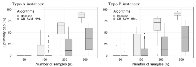
Figure 3: Optimality gaps on Type-A and Type-B instances as a function of the number of samples

As can be seen, CB-SVM-HML achieves better optimality gaps than the baseline algorithm for all values of $n$. Especially when $n=500$, the baseline method terminates with optimality gaps as high as $85\%$ in most cases, whereas CB-SVM-HML achieves much smaller gaps. This confirms the positive impact of the CB cuts, which significantly tighten the formulation and decrease the optimality gap.

4.3 Impact of the time dedicated to cut separation

Finally, we measure the impact of the amount of computational effort dedicated to separating the CB cuts on solution quality. We therefore compare eight different configurations of CB-SVM-HML with different time budgets for $T_{\textsc{S}}$ and $T_{\textsc{B}}$ to evaluate the impact of CB-cuts separation on randomized sample subsets (during $T_{\textsc{S}}$) as well as on the complete problem (during $T_{\textsc{B}}$). For all configurations, we fix the total time limit to $T_{\textsc{Max}}$ to 600 seconds. Figure 4 shows the results of this experiment as boxplots, where each plot corresponds to the optimality gaps obtained by a method configuration on an instance set. Additionally, we indicate the number of optimal solutions found by each configuration on top of each boxplot.

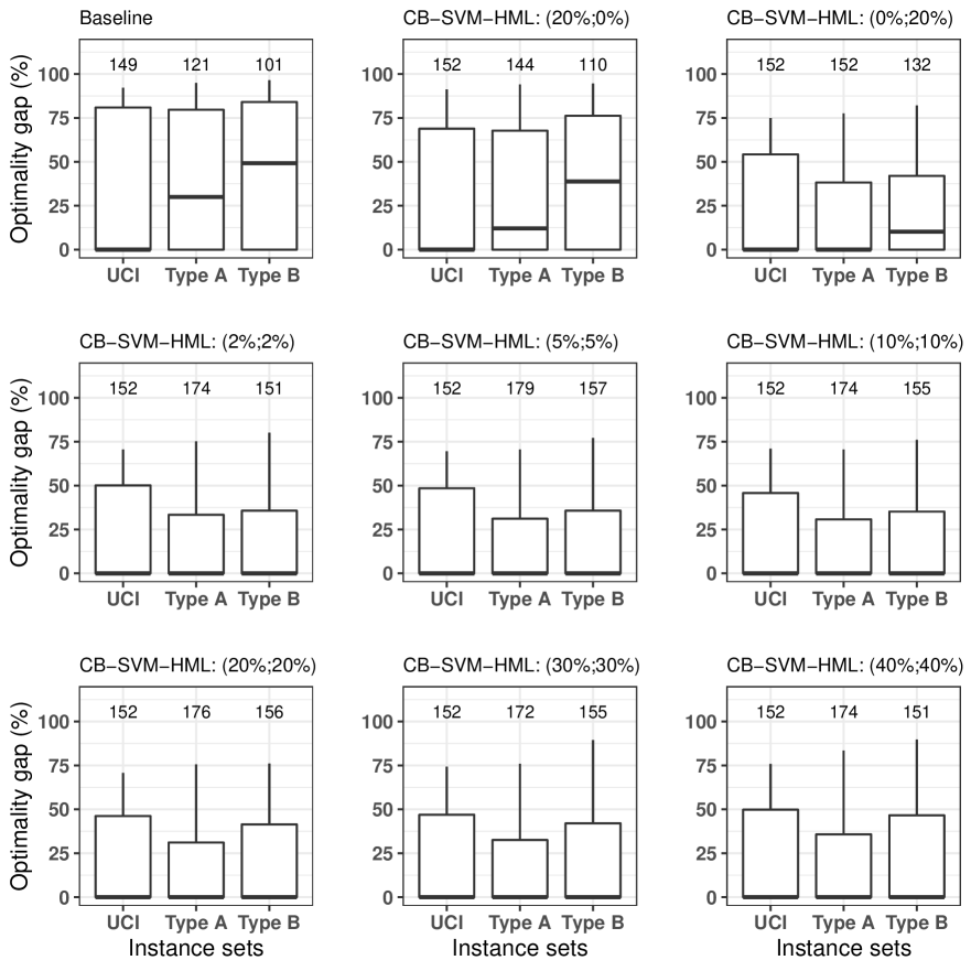
Figure 4: Optimality gaps achieved by CB-SVM-HML with different values of $T_{B}$ and $T_{S}$

As can be seen, the configuration $(5\%;5\%)$ (which is the reference configuration used in Section 4.2) achieved the best performance among all the considered configurations. Moreover, all the configurations with combinatorial Benders’ cuts achieved better gaps and number of optimal solutions than the baseline algorithm of Brooks [5]. Comparing configuration $(T_{\textsc{S}},T_{\textsc{B}})=(10\%,10\%)$ with configurations $(20\%,0\%)$ and $(0\%,20\%)$, we notice that allocating the complete separation-time budget to the complete problem or to the randomized subproblems is not as effective as dividing the available time between these two approaches. Finally, allocating a larger amount of time to the separation process, as in configurations $(30\%,30\%)$ and $(40\%,40\%)$, also leads to a performance deterioration since there is a larger number of cuts, which leads to a heavier model, such that the remaining time to solve Step 3 is insufficient to obtain a good solution quality.

As seen in Table 7, the previous observations are confirmed at $0.05$ significance level by paired-samples Wilcoxon tests. All versions of CB-SVM-HML obtained optimality gaps which were significantly smaller than the baseline method of Brooks [5] without cuts. Moreover, the configuration of CB-SVM-HML with $(T_{\textsc{S}},T_{\textsc{B}})=(5\%,5\%)$ obtained better results than all configurations, except $(20\%,20\%)$ for which no statistical difference was observed.

Table 7: Significance results of paired-samples Wilcoxon tests

Configuration		(20%,0%)	(0%,20%)	(2%,2%)	(5%,5%)	(10%,10%)	(20%,20%)	(30%,30%)	(40%,40%)
vs	p	$<$0.001	$<$0.001	$<$0.001	$<$0.001	$<$0.001	$<$0.001	$<$0.001	$<$0.001
Baseline [5]	sign	✓	✓	✓	✓	✓	✓	✓	✓
vs	p	$<$0.001	$<$0.001	$<$0.001	–	$<$0.001	0.796	$<$0.001	$<$0.001
(5%,5%)	sign	✓	✓	✓	–	✓		✓	✓

5 Conclusion

In this study, we have introduced CB-SVM-HML, a mixed integer programming approach based on combinatorial Benders’ cuts for optimally training the SVM-HML. CB-SVM-HML operates by (i) generating an initial heuristic solution of the SVM-HML to obtain an upper bound on $||w||$, (ii) using this bound to define separation subproblems that permit to separate CB cuts, and finally (iii) solving the SVM-HML with these additional cuts. Through extensive experiments, we observed that this methodology permits substantial advances in the solution of the SVM-HML, increasing our ability to achieve optimal solutions and small optimality gaps. Our sensitivity analyses show that additionally separating CB cuts on small randomized subproblems with fewer samples also permits substantial performance improvements.

The findings of our study open many research avenues. First, we suggest pursuing methodological developments on mixed-integer programming strategies for the SVM-HML. Indeed, non-convex separation problems such as the SVM-HML with natural “big-M” MILP formulations are archetypal in many classification models (see, e.g., [7, 18, 22, 24, 26, 35]), such that new developments realized on one problem can trigger significant advances for the others. Next, while this study focuses on algorithms capable of proving optimality, research is still needed on efficient heuristics that can scale up to much larger data sets. Arguably, there is a need for both optimal algorithms and heuristics, since known optimal solutions give critical information regarding our ability to solve training problems reliably. Moreover, optimal or near-optimal solutions permit us to properly assess learning models without confounding factors due to the possible errors and instabilities of the training algorithms [25]. Finally, from a more general viewpoint, combinatorial optimization techniques can play an essential role in many other learning tasks and models. Especially given the rising concerns over equity, privacy, and transparency, sophisticated optimization strategies become necessary for challenging tasks related to model compression, training, and explanations, among others [23, 38, 44, 49].

References

- Akpinar et al. [2017] Akpinar, S., A. Elmi, T. Bektaş. 2017. Combinatorial Benders cuts for assembly line balancing problems with setups. European Journal of Operational Research 259(2) 527–537.
- Baldomero-Naranjo et al. [2020] Baldomero-Naranjo, M., L.I. Martínez-Merino, A.M. Rodríguez-Chía. 2020. Tightening big Ms in integer programming formulations for support vector machines with ramp loss. European Journal of Operational Research 286(1) 84–100.
- Belotti et al. [2016] Belotti, P., P. Bonami, M. Fischetti, A. Lodi, M. Monaci, A. Nogales-Gómez, D. Salvagnin. 2016. On handling indicator constraints in mixed integer programming. Computational Optimization and Applications 65(3) 545–566.
- Benders [1962] Benders, J.F. 1962. Partitioning procedures for solving mixed variables programming problems. Numersiche Mathematik 4 238–252.
- Brooks [2011] Brooks, J.P. 2011. Support vector machines with the ramp loss and the hard margin loss. Operations Research 59(2) 467–479.
- Byun and Lee [2002] Byun, H., S.W. Lee. 2002. Applications of support vector machines for pattern recognition: a survey. International Workshop on Support Vector Machines. Springer, Berlin, Heidelberg, 213–236.
- Carrizosa et al. [2021] Carrizosa, E., C. Molero-Río, D. Romero Morales. 2021. Mathematical optimization in classification and regression trees. TOP 29(1) 5–33.
- Carrizosa and Morales [2013] Carrizosa, E., D.R. Morales. 2013. Supervised classification and mathematical optimization. Computers and Operations Research 40(1) 150–165.
- Cervantes et al. [2020] Cervantes, J., F. Garcia-Lamont, L. Rodríguez-Mazahua, A. Lopez. 2020. A comprehensive survey on support vector machine classification: applications, challenges and trends. Neurocomputing 408 189–215.
- Chang and Lin [2011] Chang, C.C., C.J. Lin. 2011. LIBSVM: a library for support vector machines. ACM Transactions on Intelligent Systems and Technology 2(3).
- Chen and Mangasarian [1996] Chen, Chunhui, O. L. Mangasarian. 1996. Hybrid misclassification minimization. Advances in Computational Mathematics 5(1) 127–136.
- Codato and Fischetti [2006] Codato, G., M. Fischetti. 2006. Combinatorial Benders’ cuts for mixed-integer linear programming. Operations Research 54(4) 756–766.
- Collobert and Bengio [2001] Collobert, R., S. Bengio. 2001. SVMTorch: Support vector machines for large-scale regression problems. Journal of Machine Learning Research 1 143–160.
- Collobert et al. [2006] Collobert, R., F. Sinz, J. Weston, L. Bottou. 2006. Trading convexity for scalability. Proceedings of the 23rd International Conference on Machine Learning 201–208.
- Côté et al. [2014] Côté, J.F., M. Dell’Amico, M. Iori. 2014. Combinatorial Benders’ cuts for the strip packing problem. Operations Research 62(3) 643–661.
- Cristianini and Shawe-Taylor [2000] Cristianini, N., J. Shawe-Taylor. 2000. An introduction to support vector machines and other kernel-based learning methods. Cambridge University Press, Cambridge.
- Dua and Graff [2017] Dua, D., C. Graff. 2017. UCI machine learning repository.
- Elizondo [2006] Elizondo, D. 2006. The linear separability problem: Some testing methods. IEEE Transactions on Neural Networks 17(2) 330–344.
- Erdoğan et al. [2015] Erdoğan, G., M. Battarra, R. Wolfler Calvo. 2015. An exact algorithm for the static rebalancing problem arising in bicycle sharing systems. European Journal of Operational Research 245(3) 667–679.
- Fan et al. [2005] Fan, R.E., P.H. Chen, C.J. Lin. 2005. Working set selection using second order information for training support vector machines. Journal of Machine Learning Research 6 1889–1918.
- Feurer et al. [2015] Feurer, M., A. Klein, K. Eggensperger, J. Springenberg, M. Blum, F. Hutter. 2015. Efficient and robust automated machine learning. Advances in Neural Information Processing Systems 28 2962–2970.
- Florio et al. [2022] Florio, A.M., P. Martins, M. Schiffer, T. Serra, T. Vidal. 2022. Optimal decision diagrams for classification. Tech. rep., arXiv:2205.14500.
- Forel et al. [2022] Forel, A., A. Parmentier, T. Vidal. 2022. Robust counterfactual explanations for random forests. Tech. rep., arXiv:2205.14116.
- Fréville et al. [2010] Fréville, A., S. Hanafi, F. Semet, N. Yanev. 2010. A tabu search with an oscillation strategy for the discriminant analysis problem. Computers & Operations Research 37(10) 1688–1696.
- Gribel and Vidal [2019] Gribel, D., T. Vidal. 2019. HG-means: A scalable hybrid metaheuristic for minimum sum-of-squares clustering. Pattern Recognition 88 569–583.
- Hanafi and Yanev [2011] Hanafi, S., N. Yanev. 2011. Tabu search approaches for solving the two-group classification problem. Annals of Operations Research 183(1) 25–46.
- Hooker and Ottosson [2003] Hooker, N., G. Ottosson. 2003. Logic-Based Benders Decomposition. Mathematical Programming, Series A 96 33–60.
- Huang et al. [2019] Huang, L.W., Y.H. Shao, J. Zhang, Y.T. Zhao, J.Y. Teng. 2019. Robust Rescaled Hinge Loss Twin Support Vector Machine for Imbalanced Noisy Classification. IEEE Access 7 65390–65404.
- Huang et al. [2014] Huang, X., L. Shi, J.A.K. Suykens. 2014. Ramp loss linear programming support vector machine. Journal of Machine Learning Research 15(1) 2185–2211.
- Joachims [1999] Joachims, T. 1999. Making large-scale SVM learning practical. Advances in Kernel Methods. MIT Press, Cambridge, MA, USA, 169–184.
- Kearns and Vazirani [1994] Kearns, M.J., U.V. Vazirani. 1994. An Introduction to Computational Learning Theory. MIT Press, Cambridge, MA.
- Lee and Huang [2007] Lee, Y.J., S.Y. Huang. 2007. Reduced support vector machines: a statistical theory. IEEE Transactions on Neural Networks 18(1) 1–13.
- Loosli et al. [2007] Loosli, G., S. Canu, L. Bottou. 2007. Training invariant support vector machines using selective sampling. Large Scale Kernel Machines 2.
- Mavroforakis and Theodoridis [2006] Mavroforakis, M.E., S. Theodoridis. 2006. A geometric approach to support vector machine (SVM) classification. IEEE Transactions on Neural Networks 17(3) 671–682.
- Murthy et al. [1994] Murthy, S. K., S. Kasif, S. Salzberg. 1994. A system for induction of oblique decision trees. Journal of Artificial Intelligence Research (2) 2(1) 1–32.
- Orsenigo and Vercellis [2003] Orsenigo, C., C. Vercellis. 2003. Multivariate classification trees based on minimum features discrete support vector machines. IMA Journal of Management Mathematics 14(3) 221–234.
- Orsenigo and Vercellis [2004] Orsenigo, Carlotta, Carlo Vercellis. 2004. Discrete support vector decision trees via tabu search. Computational Statistics and Data Analysis 47(2) 311–322.
- Parmentier and Vidal [2021] Parmentier, A., T. Vidal. 2021. Optimal counterfactual explanations in tree ensembles. M. Meila, T. Zhang, eds., Proceedings of the 38th International Conference on Machine Learning. Proceedings of Machine Learning Research, PMLR, Virtual, 8422–8431.
- Pérez-Cruz et al. [2003] Pérez-Cruz, F., A. Navia-Vázquez, A.R. Figueiras-Vidal, A. Artés-Rodríguez. 2003. Empirical risk minimization for support vector classifiers. IEEE Transactions on Neural Networks 14(2) 296–303.
- Platt [1999] Platt, J. 1999. Fast training of support vector machines using sequential minimal optimization. Advances in Kernel Methods — Support Vector Learning. MIT Press, Cambridge, MA, 185–208.
- Poursaeidi and Kundakcioglu [2014] Poursaeidi, M.H., O.E. Kundakcioglu. 2014. Robust support vector machines for multiple instance learning. Annals of Operations Research 216(1) 205–227.
- Rudin [2019] Rudin, C. 2019. Stop explaining black box machine learning models for high stakes decisions and use interpretable models instead. Nature Machine Intelligence 1(5) 206–215.
- Schölkopf et al. [2002] Schölkopf, B., A.J. Smola, F. Bach. 2002. Learning with Kernels: Support Vector Machines, Regularization, Optimization, and Beyond. MIT Press, Cambridge, MA.
- Serra et al. [2020] Serra, T., A. Kumar, S. Ramalingam. 2020. Lossless compression of deep neural networks. E. Hebrard, N. Musliu, eds., CPAIOR 2020: Integration of Constraint Programming, Artificial Intelligence, and Operations Research. Springer, 417–430.
- Shawe-Taylor et al. [2004] Shawe-Taylor, J., N. Cristianini, et al. 2004. Kernel methods for pattern analysis. Cambridge university press.
- Shen et al. [2003] Shen, X., G.C. Tseng, X. Zhang, W.H. Wong. 2003. On -learning. Journal of the American Statistical Association 98(463) 724–734.
- Vapnik [1998] Vapnik, V.N. 1998. Statistical Learning Theory. Wiley, New York.
- Vidal et al. [2019] Vidal, T., D. Gribel, P. Jaillet. 2019. Separable convex optimization with nested lower and upper constraints. INFORMS Journal on Optimization 1(1) 71–90.
- Vidal and Schiffer [2020] Vidal, T., M. Schiffer. 2020. Born-again tree ensembles. Hal Daumé III, Aarti Singh, eds., Proceedings of the 37th International Conference on Machine Learning, Proceedings of Machine Learning Research, vol. 119. PMLR, Virtual, 9743–9753.
- Wang et al. [2020] Wang, Q., Y. Ma, K. Zhao, Y. Tian. 2020. A comprehensive survey of loss functions in machine learning. Annals of Data Science 1–26.
- Wang and Xu [2004] Wang, W., Z. Xu. 2004. A heuristic training for support vector regression. Neurocomputing 61 259–275.
- Wolsey [2020] Wolsey, L. A. 2020. Integer Programming. John Wiley & Sons, Ltd.
- Wu and Liu [2007] Wu, Y., Y. Liu. 2007. Robust truncated hinge loss support vector machines. Journal of the American Statistical Association 102(479) 974–983.
- Xu et al. [2009] Xu, H., C. Caramanis, S. Mannor. 2009. Robustness and regularization of support vector machines. Journal of Machine Learning Research 10 1485–1510.