Aberration-Corrected Time Aperture of an Electro-Optic Time Lens

Abstract

Recently, there has been renewed interest in electro-optic time lenses due to their favorable properties for quantum photonic applications. Here, we propose a new analytical approach to estimate the chirp rate of a time lens implemented using an electro-optic phase modulator driven with a single-tone radio frequency voltage. Our approach is based on a user-defined time aperture for the time lens. We observe that the temporal aberrations depend on the amplitude of the phase modulation and the effective time aperture of the time lens. We derive an analytical expression for the maximum phase error that will allow the user to choose the maximal aberration-limited time aperture of the time lens. We apply our formalism to a Fourier-time lens system for the spectral compression of Gaussian pulses and find the optimal parameters of the setup. Our approach will provide a handy tool for efficient temporal system design based on electro-optical time lenses.

I Introduction

Temporal systems based on optical space-time duality – an analogy between the diffraction of a paraxial optical beam and the dispersion of a narrow-band pulse Kolner (1994), have revolutionized the detection and manipulation of ultra-fast optical signals Torres-Company et al. (2011); Salem et al. (2013). For example, temporal imaging, time-to-frequency conversion, or vice versa Kolner (1989); Azaña (2003), are essential tools in contemporary optical communication van Howe and Xu (2006). Recently, applications of temporal optics have been extended to quantum light, which opens up, e.g., new tool for ultrafast signal processing at single photon level Tsang and Psaltis (2006); Patera et al. (2017). Moreover, efficient bandwidth manipulation of single-photon pulses have been demonstrated with electro-optic time lens Karpiński et al. (2017); Sośnicki et al. (2020). Developing new practical quantum technologies based on ST duality requires tools for system design which account for aberrations Tsang and Psaltis (2006); Kielpinski et al. (2011); Zhu et al. (2013); Lavoie et al. (2013); Donohue et al. (2016); Patera et al. (2017); Mittal et al. (2017); Karpiński et al. (2017); Sośnicki et al. (2020); Karpiński et al. (2021).

In diffraction optics, many tasks can be achieved with a simple lens or a combination of lenses. Similarly, a time lens is an essential component of temporal systems. It is a device that imparts a time-dependent quadratic phase on an optical pulse, which chirps the pulse linearly. First demonstrated with an electro-optic phase modulator (EOPM) in traveling-wave configuration by Kolner in 1988 Kolner (1988), where the necessary quadratic phase is provided locally by the driving sinusoidal voltage. We will refer to this particular implementation as a sinusoidal time lens. With analogy to space-time (ST) duality, he also derived an equivalent focal ‘length’ and f-number for the sinusoidal time lens Kolner (1989). Since then, many implementations of the time lens have been shown with non-linear processes Bennett and Kolner (2000); Foster et al. (2008, 2009); Li et al. (2015). However, the electro-optic approach remains popular because of its easy reconfiguration, wavelength-preserving operation, and deterministic nature of phase imprinting. These properties make it attractive for quantum interface applications Karpiński et al. (2017); Sośnicki et al. (2020); Karpiński et al. (2021).

The real time lens systems have a finite time aperture, i.e., the time window in which the phase is approximately quadratic. The deviations from the ideal quadratic phase profile (phase error) of the time lens result in distortions (or aberrations) in the output pulse spectrum. Aberrations in parametric time lenses and four-wave mixing time lens systems have been studied Bennett and Kolner (2001); Schröder et al. (2010); Duadi et al. (2021). It is known that the use of longer input pulses with the sinusoidal time lens results in distortions in the output pulse spectrum Kolner (1988), but it was never thoroughly studied. Aberrations limit the usable time aperture of a time lens system, and hence the resolving power Salem et al. (2013); Tsang and Psaltis (2006).

There have been several attempts to minimize the phase error while extending the time aperture of an electro-optic time lens. One way is to implement a Fresnel-type time lens which involves phase wrapping around every integral multiple (order) of $2\pi$ Sośnicki and Karpiński (2018); Zhang et al. (2019). This requires a complicated electronic signal to drive the EOPM, and the time aperture depends on the bandwidth of the arbitrary waveform generator and the order of the phase wrapping. Another way is to add a few higher harmonics to the fundamental driving signal with weighted amplitudes and phases to minimize phase error in a user-defined time aperture van Howe et al. (2004); Wu et al. (2010); Munioz-Camuniez et al. (2010). This approach results in a high peak voltage of the deriving signal, effectively increasing the RF power consumed by the EOPM. Both approaches significantly improve the time aperture but require broadband electronics, making the experimental realization complex and expensive. The single-tone operation of the sinusoidal time lens makes its implementation and reconfiguration simple.

Here, we propose an analytical expression for the chirp rate of the sinusoidal time lens for a user-defined time aperture. We analyze the phase error as a function of the time aperture and present a closed-form expression for the maximal phase error. Then we apply our formalism to spectral bandwidth compression of Gaussian-shaped pulses and propose a procedure to find an upper limit on the time aperture for a given setting of the sinusoidal time lens.

II Theory

The function of an ideal time lens is to imprint a time-varying quadratic phase,

$$\phi(t)=\frac{1}{2}Kt^{2},$$ (1)

across an optical pulse, here $K$ is the chirp rate. The first experimental implementation of a time lens was demonstrated using an electro-optic phase modulator driven with a single-tone radio frequency (RF) signal. These modulators work on the principle of Pockel’s effect, in which the refractive index of the electro-optic crystal changes linearly with the applied electric field Saleh and Teich (2019). In the traveling-wave configuration and in the absence of velocity mismatch, the optical pulse and the driving RF signal co-propagate in the modulator. If the center of the optical pulse is synchronized with an extremum of the RF signal, the phase acquired by the pulse is given by

$$\theta(t)=\pm A\cos(\omega_{m}t),$$ (2)

here $\omega_{m}$ is the angular frequency of the modulating RF signal and $A$ is the phase modulation amplitude. The sign of phase modulation depends on whether a maximum or minimum of the RF signal is synchronized with the pulse center. The modulation amplitude $A$ depends on the amplitude of the applied RF voltage $V_{m}$,

$$A=\frac{\pi V_{m}}{V_{\pi}},$$ (3)

where $V_{\pi}$ is the half-wave voltage. Practically, the maximum modulation amplitude of an EOPM depends on the modulation frequency and is limited by the breakdown voltage of the modulator and thermal effects. But these details are not relevant to our discussion.

If the duration of the optical pulse is much shorter than the period of the RF signal, then the phase modulation can be approximated with the Taylor expansion of the RF drive around the cusp,

$$\theta(t)=\pm A\left(1-\frac{\omega_{m}^{2}}{2!}t^{2}+\frac{\omega_{m}^{4}}{4!}t^{4}-\cdots\right).$$ (4)

We can ignore the first constant term in the expansion, since it will introduce only a constant phase shift to the pulse. Around the cusp, higher-order terms can be ignored, and the phase is approximately quadratic,

$$\theta(t)\approx\mp\frac{1}{2}A\omega_{m}^{2}t^{2},$$ (5)

implementing a time lens. A direct comparison with Eq. (1) gives the chirp rate $K_{\text{std}}=A\omega_{m}^{2}$. Here, we will refer to it as the standard chirp rate. This is the standard formula used extensively in the literature Kolner (1994); Torres-Company et al. (2011); Salem et al. (2013). Using pulses with a longer duration introduces aberrations in the spectrum of the optical pulse. There is no well-defined value of the time aperture for the sinusoidal time lens. However, for a clean output spectrum, it is widely accepted that it is $1/\omega_{m}$, which is about $17\%$ of the driving RF signal period Kolner (1988, 1989); Kauffman et al. (1993); Kolner (1994); Bennett and Kolner (2001); van Howe et al. (2004); van Howe and Xu (2006); Fernández-Pousa (2006); Li and Azaña (2007a, b); Costanzo-Caso et al. (2008); Munioz-Camuniez et al. (2010); Torres-Company et al. (2011); Salem et al. (2013); Zhang et al. (2013); Plansinis et al. (2015); Mittal et al. (2017); Zhu et al. (2021).

We define the time aperture ($\tau_{a}$) of the sinusoidal time lens based on a user-defined fraction of the period ($T=2\pi/\omega_{m}$) of the modulating RF signal, parameterized with a dimensionless aperture parameter $\alpha$ (similar to what is described in Ref. Munioz-Camuniez et al. (2010)) as

$$\tau_{a}=\alpha T,$$ (6)

where $\alpha\in(0,1]$.

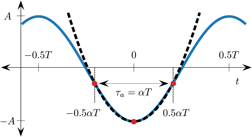
Figure 1: Illustration of the idea of aperture-parameter-dependent ($\alpha$) chirp rate approximation for the sinusoidal time lens. The two symmetric points (red dots) around $t=0$ define the time aperture ($\tau_{a}$) as a fraction of the time period ($\alpha$T). The black dashed line is the unique quadratic function passing through the center and the edges of the time aperture. $A$ is the modulation amplitude and $T$ is the period of the sinusoidal phase (blue solid line).

We demand the time lens to be centered at $t=0$, and pass through the edges of the time aperture on the modulating sinusoidal phase, as illustrated in Fig. 1. Now we find the equation of the unique quadratic function passing through these three points, resembling Eq. (1), which gives the chirp rate,

$$K(\alpha)=\mp A\omega_{m}^{2}\text{sinc}^{2}(\alpha\pi/2).$$ (7)

In the limit of vanishing aperture parameter

$$\lim_{\alpha\to 0}K(\alpha)=\mp A\omega_{m}^{2}=K_{\text{std}},$$ (8)

we obtain the standard chirp rate derived earlier using the Taylor expansion, which shows the consistency of our approach with the standard approximation. The approximated chirp rate represents an ideal time lens of the chirp rate $K(\alpha)$ and time aperture $\alpha T$, see Fig. 2(a). Of course, sinusoidal modulation provides a quasi-quadratic phase with some deviations from the estimated ideal quadratic phase, which causes aberrations in a temporal system. The phase error in our case is given by

$$\begin{split}\Delta\theta(t/T,\alpha)&=A\Bigg{[}-\cos(\frac{2\pi}{T}t)\\ &-\frac{1}{2}\text{sinc}^{2}\left(\frac{\alpha\pi}{2}\right)\left(\frac{2\pi}{T}t\right)^{2}+1\Bigg{]}.\end{split}$$ (9)

It is evident from Eq. (9) that the phase error is linearly dependent on the modulation amplitude. Note that it is independent of the modulation frequency and is a function of the fraction of the time period $t/T$, for a given aperture parameter. In Fig. 2(b), we show the numerically evaluated phase error for some values of the aperture parameter and compare with the phase error from the standard approximation. It is visually clear that our approach provides a smaller phase error within the defined time aperture marked with thin-dashed vertical lines.

For many applications, it is sufficient to consider the peak-to-peak phase error in the desired temporal window. By construction of our approximation, we get zero phase error at the center and edges of the time aperture. We numerically find the position of the maximum phase error (see Fig. 2c), which can be approximated with a linear function of the aperture parameter. Now the maximum phase error can be evaluated as a function of the aperture parameter,

$$\Delta\theta(\alpha,A)_{\text{max}}=2A[\sin^{2}(\pi\gamma\alpha)-4\gamma^{2}\sin^{2}(\alpha\pi/2)],$$ (10)

where $\gamma=\pm 0.347$, which comes from the linear approximation for the position of the maximum phase error. We compare the maximum phase error percent of the modulation amplitude within the defined time aperture, resulting from our approximation against the standard approximation in Fig. 2(d), and we draw two conclusions, (i) for a given modulation amplitude, using our approximation, one can always use a higher aperture than the standard approximation allows for a similar maximum phase error. (ii) For a fixed maximum phase error, one can use a higher aperture for a smaller modulation amplitude.

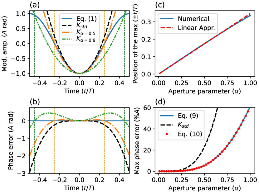
Figure 2: (a) The sinusoidal modulation (solid blue line) and estimated quadratic phases for $\alpha=0.5$ (orange, dotted-dashed line), $\alpha=0.9$ (green, double-dotted-dashed line), and standard formula (black bashed line) and corresponding phase error is plotted in (b), the thin-dashed vertical lines mark the time aperture. (c) Blue solid line is the numerically evaluated position of the maximum phase error as a function of the aperture parameter and red dashed line the linear approximation. (d) Comparison of maximum phase error (percent of the modulation amplitude), as a function of the aperture parameter (blue solid line is the numerical solution) and with the standard chirp rate (black dashed line). The red filled-circles show the approximation for the max phase error described by Eq. (10).

The user can choose the aperture parameter according to the modulation amplitude requirement of the system under design and the allowed tolerance for the maximum phase error.

III Spectral bandwidth compression of Gaussian pulses

So far, the analysis has been independent of any temporal-optical system. Now, we apply the aperture parameter-based formalism to spectral bandwidth compression of Gaussian-shaped pulses with a system of parabolic dispersive medium followed by a sinusoidal time lens. In analogy with ST duality, the propagation distance in diffraction optics corresponds to the group delay dispersion (GDD) in temporal optics. After propagating through a dispersive medium with GDD $\Phi$, a transform-limited (unchirped) pulse expands in time and acquires a linear chirp with the chirp rate $1/\Phi$ Saleh and Teich (2019). A time lens with equal and opposite chirp ($K=-1/\Phi$) is used to unchirp the pulse, resulting in compression of the spectral bandwidth, schematically illustrated in Fig. 3. The latter setup is the temporal equivalent of spatial beam collimation with a thin lens, with

$$K=-\frac{1}{\Phi},$$ (11)

being the collimation condition.

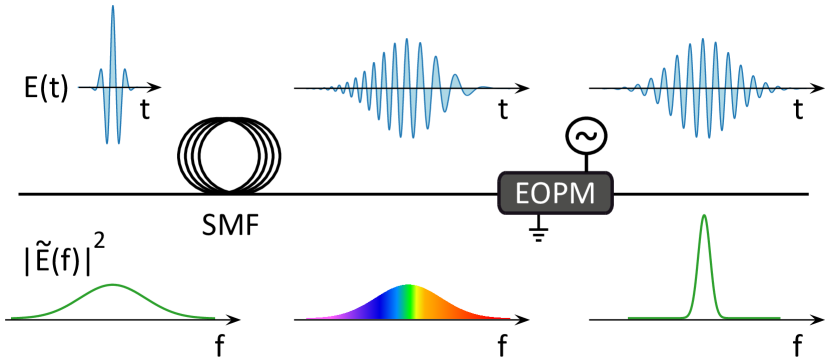
Figure 3: Schematic of the spectral bandwidth compression setup. A spool of single mode fiber (SMF) introduces the desired group delay dispersion (GDD), which stretches and chirps the pulse. An electro-optic phase modulator (EOPM) driven with a sinusoidal voltage (acting as a time lens) is used to imprint the temporal quadratic phase on the optical pulse, which corrects the chirp introduced by GDD. For Gaussian pulses this setup results in bandwidth compression. The optical cycles in the pulses are not to scale.

Due to the non-ideal quadratic phase and the not well-defined time aperture of the sinusoidal time lens, disagreements have been noticed in balancing the GDD, the chirp rate and the input bandwidth Costanzo-Caso et al. (2008); Karpiński et al. (2017); Zhu et al. (2021). Here, our goal is to find the aperture parameter which gives the optimal collimation condition and to find the optimal input bandwidth which fills the aperture (within some measure of the aberrations) for a given modulation amplitude.

Before proceeding with the analysis, let us define some useful quantities. One of the quantities of interest in such experiments is the enhancement of optical power at the carrier frequency ($f_{0}$) of the pulse, which can be conveniently defined as follows.

$$\eta=\frac{\delta f_{\text{in}}}{\delta f_{\text{out}}},$$ (12)

where $\delta f_{\text{in(out)}}$ is the power equivalent bandwidth (PEB) of the input (output) pulse. The power equivalent bandwidth itself is defined by

$$\delta f=\frac{\int_{-\infty}^{\infty}|\tilde{E}{(f)}|^{2}df}{|\tilde{E}{(f_{0})}|^{2}},$$ (13)

where $|\tilde{E}{(f)}|^{2}$ is the spectral intensity Saleh and Teich (2019). In our analysis, we used the normalized Gaussian spectral intensity, so the PEB is simply the inverse of the peak spectral intensity.

As an example, let us try to find the optimal $\alpha$ and $\Delta f_{\text{in}}$ (full width at half maximum) for a fixed setting of the sinusoidal time lens ($A=4\pi$, $\omega_{m}=2\pi\times 10$ GHz), which results in the narrowest PEB. We numerically generate a color map for PEB, considering Gaussian pulses with different full-width half-maximum (FWHM) bandwidth and dispersing it with different amounts of GDD. The output PEB is shown in Fig. 4(a), which shows that the line of minimum PEB (solid white line) is much further from the standard approximation (the black dashed line). For large $\Delta f_{\text{in}}$, the minimum PEB corresponds to $\alpha=0.56$, shown as a blue dashed dotted line. We compare the enhancement along the two collimation conditions in Fig. 4(b). It is clear that the new approximation provides much better enhancement than the standard approximation. In both cases, the enhancement and output FWHM bandwidth asymptotically saturates, see Fig. 4(c), whereas the PEB along the two lines starts to broaden after exhibiting a minimum (see Fig. 4d). The broadening of PEB indicates the energy distribution into the side bands due to aberrations. The ratio of PEB and FWHM widths can serve as a good quantifier for distortions in the spectrum. So, we define quality of compression as

$$Q=\frac{\Delta f_{\text{out}}}{\xi\delta f_{\text{out}}},$$ (14)

where $\Delta f_{\text{out}}$ is the FWHM bandwidth of the output spectrum and $\delta f_{\text{out}}$ is the PEB of the output spectrum. The value of $\xi\approx 1.06$, is the ratio of PEB and FWHM of a Gaussian pulse. The value of $Q=1$ indicates aberration-free compression, and $Q<1$ indicates distortions in the output spectrum due to aberrations; see Fig. 4(e).

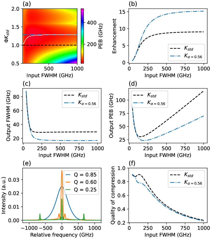
Figure 4: An example for comparing the standard approximation and the new approximation for fixed modulation parameters ($A=4\pi$, $\omega_{m}=2\pi\times 10$ GHz). (a) Output power-equivalent width as a function of group delay dispersion and input bandwidth. The solid white line marks the line of minimum PEB. The black dashed line shows the standard collimation condition and the blue dotted-dashed line shows the collimation condition for $\alpha=0.56$. (b) Enhancement, (c) full width half maximum output bandwidth, (d) output power-equivalent bandwidth, and (e) ouput spectra for selected quality of compression. Q = 0.85 (blue), Q = 0.60 (orange), and Q = 0.25 (green). (f) Quality of compression, along the standard collimation condition and with new approximation.

The quality of compression along the two collimation conditions is shown in Fig. 4(f). The quality of compression decreases with increasing input bandwidth. For high input bandwidths, the compression quality for both approximations is almost the same, which means that our approximation provides almost double enhancement with a similar quality for the analyzed case of modulation amplitude $4\pi$, which is typically available from the standard waveguide EOPMs.

As we have established earlier, the time aperture depends on the modulation amplitude for a given quality of compression. Deciding on the aperture parameter means that we fix the chirped pulse duration as the pulse needs to fill the aperture. A Gaussian pulse with spectral bandwidth $\Delta f_{\text{in}}$ (FWHM) after dispersive propagation broadens to a new pulse duration $\Delta t_{\text{out}}$. The duration of the dispersed pulse $\Delta t_{\text{out}}$ in the large GDD regime is given by

$$\Delta t_{\text{out}}=2\pi\Delta f_{\text{in}}\Phi.$$ (15)

We equate the duration of the dispersed pulse $\Delta t_{\text{out}}$ with the time aperture of the sinusoidal time lens, and from the collimation condition, Eq. (11), and Eq. (7) we can write

$$\alpha T=\frac{2\pi\Delta f_{\text{in}}}{A\omega_{m}^{2}\text{sinc}^{2}(\alpha\pi/2)}.$$ (16)

Solving for $\Delta f_{\text{in}}$, we obtain

$$\Delta f_{\text{in}}=A\alpha\omega_{m}\text{sinc}^{2}(\alpha\pi/2).$$ (17)

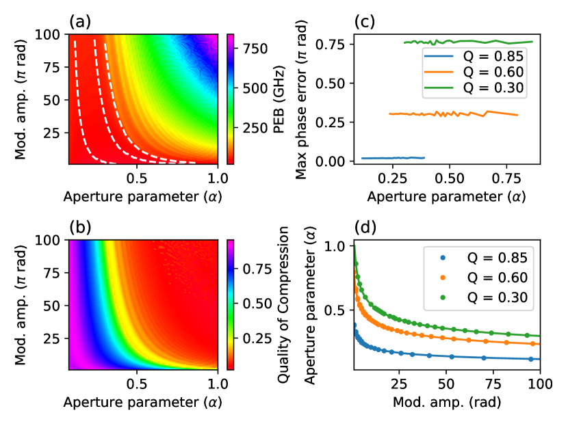
Figure 5: (a) Power-equivalent bandwidth map, and (b) quality of compression map as function of modulation amplitude and the aperture parameter. The white dashed lines in (a) are the constant quality of compression lines for Q = 0.85, Q = 0.60, and Q = 0.25. (c) Maximum phase error for selected quality of compression. (d) The relationship of modulation amplitude and aperture parameter which leads to a constant quality of compression.

Equation (17) relates the input bandwidth to the time lens parameters, which is of practical importance because it will allow the user to find the input bandwidth that will fully utilize the aperture.

We calculate the input bandwidth according to Eq. (17) for a fixed modulation frequency ($\omega_{m}=2\pi\times 10$ GHz), and using the collimation condition (Eq. 11), we estimate the GDD. The results are shown in Fig. 5. The output PEB is shown in Fig. 5(a) and the quality of compression is shown in Fig. 5(b). The white lines show the constant quality of compression, which corresponds to the quality (aberration)-limited aperture for a given modulation amplitude. The phase error along the marked lines of constant Q is shown in Fig. 5(c). We observe that the quality of compression is related to the absolute maximum phase error regardless of the modulation amplitude and the aperture parameter. This means that we can choose $\alpha$ for a given modulation amplitude using Eq. (10), once agreed on the quality of compression desired by the application.

The relationship between the aperture parameter and the modulation amplitude for a given quality of compression is plotted in Fig. 5(d). This offers a scheme to choose quality-limited aperture parameter for a given modulation amplitude.

IV Summary

We developed a new analytical formalism to estimate the chirp rate of a sinusoidal time lens for a user-defined time aperture. We characterize the temporal aberrations as a function of the time aperture. By applying our formalism to bandwidth compression of Gaussian-shaped pulses with a system of a GDD medium and a sinusoidal time lens, we show almost double enhancement of spectral intensity in comparison to the standard approach. We also provide a procedure to choose the quality-limited aperture parameter. Given the growing interest of applications of electro-optic phase modulation in quantum information science, our formalism will serve a handy system design tool for the development of efficient systems based on sinusoidal time lenses.

References

- Kolner (1994) B. H. Kolner, “Space-time duality and the theory of temporal imaging,” IEEE J. Quantum Electron. 30, 1951–1963 (1994).
- Torres-Company et al. (2011) V. Torres-Company, J. Lancis, and P. Andrés, “Space-time analogies in optics,” Prog. Opt. 56, 1–80 (2011).
- Salem et al. (2013) R. Salem, M. A. Foster, and A. L. Gaeta, “Application of space–time duality to ultrahigh-speed optical signal processing,” Adv. Opt. Photonics 5, 274–317 (2013).
- Kolner (1989) Brian H. Kolner, “Temporal imaging with a time lens,” Opt. Lett. 14, 630–632 (1989).
- Azaña (2003) José Azaña, “Time-to-frequency conversion using a single time lens,” Opt. Commun. 217, 205–209 (2003).
- van Howe and Xu (2006) James van Howe and Chris Xu, “Ultrafast optical signal processing based upon space-time dualities,” J. Light. Technol. 24, 2649–2662 (2006).
- Tsang and Psaltis (2006) Mankei Tsang and Demetri Psaltis, “Propagation of temporal entanglement,” Phys. Rev. A 73, 013822 (2006).
- Patera et al. (2017) G. Patera, , J. Shi, D. B. Horoshko, and M.I. Kolobov, “Quantum temporal imaging: application of a time lens to quantum optics,” J. Opt 19, 054001 (2017).
- Karpiński et al. (2017) M. Karpiński, M. Jachura, L. J. Wright, and B. J. Smith, “Bandwidth manipulation of quantum light by an electro-optic time lens,” Nat. Photon. 11, 53–57 (2017).
- Sośnicki et al. (2020) Filip Sośnicki, Michał Mikołajczyk, Ali Golestani, and Michał Karpiński, “Aperiodic electro-optic time lens for spectral manipulation of single-photon pulses,” Appl. Phys. Lett. 116, 234003 (2020).
- Kielpinski et al. (2011) D. Kielpinski, J. F. Corney, and H. M. Wiseman, “Quantum optical waveform conversion,” Phys. Rev. Lett. 106, 130501 (2011).
- Zhu et al. (2013) Yunhui Zhu, Jungsang Kim, and Daniel J. Gauthier, “Aberration-corrected quantum temporal imaging system,” Phys. Rev. A 87, 043808 (2013).
- Lavoie et al. (2013) J. Lavoie, J. M. Donohue, L. G. Wright, A. Fedrizzi, and K. J. Resch, “Spectral compression of single photons,” Nat. Photonics 7, 363–366 (2013).
- Donohue et al. (2016) J. M. Donohue, M. Mastrovich, and K. J. Resch, “Spectrally engineering photonic entanglement with a time lens,” Phys. Rev. Lett. 117, 243602 (2016).
- Mittal et al. (2017) S. Mittal, V. V. Orre, A. Restelli, R. Salem, E. A. Goldschmidt, and M. Hafezi, “Temporal and spectral manipulations of correlated photons using a time lens,” Phys. Rev. A 96, 043807 (2017).
- Karpiński et al. (2021) Michał Karpiński, Alex O. C. Davis, Filip Sośnicki, Valérian Thiel, and Brian J. Smith, “Control and measurement of quantum light pulses for quantum information science and technology,” Adv. Quantum Technol. 4, 2000150 (2021).
- Kolner (1988) Brian H. Kolner, “Active pulse compression using an integrated electro-optic phase modulator,” Appl. Phys. Lett. 52, 1122–1124 (1988).
- Bennett and Kolner (2000) C. V. Bennett and B. H. Kolner, “Principles of parametric temporal imaging. i. system configurations,” IEEE J. Quantum Electron. 36, 430–437 (2000).
- Foster et al. (2008) M. A. Foster, R. Salem, D. G. Geraghty, A. C. Turner-Foster, M. Lipson, and A. L. Geata, “Silicon-chip-based ultrafast optical oscilloscope,” Nature 456, 81–83 (2008).
- Foster et al. (2009) M. A. Foster, R. Salem, Y. Okawachi, A. C. Turner-Foster, M. Lipson, and A. L. Geata, “Ultrafast waveform compression using a time-domain telescope,” Nat. Photonics 3, 581–585 (2009).
- Li et al. (2015) Bo Li, Ming Li, and José Azaña, “Temporal imaging of incoherent-light intensity waveforms based on a gated time-lens system,” IEEE Photonics J. 7, 1943–0655 (2015).
- Bennett and Kolner (2001) C. V. Bennett and B. H. Kolner, “Aberrations in temporal imaging,” IEEE J. Quantum Electron. 37, 20–32 (2001).
- Schröder et al. (2010) Jochen Schröder, Fan Wang, Aisling Clarke, Eva Ryckeboer, Mark Pelusi, Michaël A. F. Roelens, and Benjamin J. Eggleton, “Aberration-free ultra-fast optical oscilloscope using a four-wave mixing based time lens,” Opt. Commun. 283, 2611–2614 (2010).
- Duadi et al. (2021) Hamootal Duadi, Avi Klein, Inbar Sibony, Sara Meir, and Moti Fridman, “Cross-phase modulation aberrations in time lenses,” Opt. Lett. 46, 3255–3258 (2021).
- Sośnicki and Karpiński (2018) Filip Sośnicki and Michał Karpiński, “Large-scale spectral bandwidth compression by complex electro-optic temporal phase modulation,” Opt. Express 26, 31307–31315 (2018).
- Zhang et al. (2019) Bowen Zhang, Dan Zhu, Yamei Zhang, and Shilong Pan, “Time lens with improved aperture to resolution ratio based on a phase modulator,” in 2019 PhotonIcs & Electromagnetics Research Symposium - Spring (PIERS-Spring) (2019) pp. 4311–4314.
- van Howe et al. (2004) James van Howe, Jonas Hansryd, and Chris Xu, “Multiwavelength pulse generator using time-lens compression,” Opt. Lett. 29, 1470–1472 (2004).
- Wu et al. (2010) Rui Wu, V. R. Supradeepa, Christopher M. Long, Daniel E. Leaird, and Andrew M. Weiner, “Generation of very flat optical frequency combs from continuous-wave lasers using cascaded intensity and phase modulators driven by tailored radio frequency waveforms,” Opt. Lett. 35, 3234–3236 (2010).
- Munioz-Camuniez et al. (2010) Luis Enrique Munioz-Camuniez, Victor Torres-Company, Jesús Lancis, Jorge Ojeda-Castañeda, and Pedro Andrés, “Electro-optic time lens with an extended time aperture,” J. Opt. Soc. Am. B 27, 2110–2115 (2010).
- Saleh and Teich (2019) Bahaa E. A. Saleh and Malvin Carl Teich, Fundamentals of photonics, 3rd ed. (Wiley, 2019).
- Kauffman et al. (1993) M. T. Kauffman, W. C. Banyal, A. A. Godil, and D. M. Bloom, “Time-to-frequency converter for measuring picosecond optical pulses,” Appl. Phys. Lett. 64, 270–272 (1993).
- Fernández-Pousa (2006) Carlos R. Fernández-Pousa, “Temporal resolution limits of time-to-frequency transformations,” Opt. Lett. 31, 3049–3051 (2006).
- Li and Azaña (2007a) Fangxin Li and José Azaña, “Simplified system configuration for real-time fourier transformation of optical pulses in amplitude and phase,” Opt. Commun. 274, 59–65 (2007a).
- Li and Azaña (2007b) Fangxin Li and José Azaña, “Simplified system configuration for real-time Fourier transformation of optical pulses in amplitude and phase,” Opt. Commun. 274, 59–65 (2007b).
- Costanzo-Caso et al. (2008) Pablo A. Costanzo-Caso, Christian Cuadrado-Laborde, Ricardo Duchowicz, and Enrique E. Sicre, “Distortion in optical pulse equalization through phase modulation and dispersive transmission,” Opt. Commun. 281, 4001–4007 (2008).
- Zhang et al. (2013) Chi Zhang, P. C. Chui, and Kenneth K. Y. Wong, “Comparsion of state-of-art phase modulators and parametric mixers in time-lens applications uder different repetition rates,” Appl. Opt. 52, 8817–8826 (2013).
- Plansinis et al. (2015) B. W. Plansinis, W. R. Donaldson, and G. P. Agrawal, “Spectral changes induced by a phase modulator acting as a time lens,” J. Opt. Soc. Am. B 32, 1550–1554 (2015).
- Zhu et al. (2021) Di Zhu, Changchen Chen, Mengjie Yu, Linbo Shao, Yaowen Hu, C. J. Xin, Matthew Yeh, Soumya Ghosh, Lingyan He, Christian Reimer, Neil Sinclair, Franco N. C. Wong, Mian Zhang, and Marko Lončar, “Spectral control of nonclassical light using an integrated thin-film lithium niobate modulator,” Arxiv (2021).