Algorithms to estimate Shapley value feature attributions

Abstract

Feature attributions based on the Shapley value are popular for explaining machine learning models; however, their estimation is complex from both a theoretical and computational standpoint. We disentangle this complexity into two factors: (1) the approach to removing feature information, and (2) the tractable estimation strategy. These two factors provide a natural lens through which we can better understand and compare 24 distinct algorithms. Based on the various feature removal approaches, we describe the multiple types of Shapley value feature attributions and methods to calculate each one. Then, based on the tractable estimation strategies, we characterize two distinct families of approaches: model-agnostic and model-specific approximations. For the model-agnostic approximations, we benchmark a wide class of estimation approaches and tie them to alternative yet equivalent characterizations of the Shapley value. For the model-specific approximations, we clarify the assumptions crucial to each method’s tractability for linear, tree, and deep models. Finally, we identify gaps in the literature and promising future research directions.

1 Introduction

Machine learning models are increasingly prevalent because they have matched or surpassed human performance in many applications: these include Go [1], poker [2], Starcraft [3], protein folding [4], language translation [5], and more. One critical component in their success is flexibility, or expressive power [6, 7, 8], which has been facilitated by more complex models and improved hardware [9]. Unfortunately, their flexibility also makes models opaque, or challenging for humans to understand. Combined with the tendency of machine learning to rely on shortcuts [10] (i.e., unintended learning strategies that fail to generalize to unseen data), there is a growing demand for model interpretability [11]. This demand is reflected in increasing calls for explanations by diverse regulatory bodies, such as the General Data Protection Regulation’s “right to explanation” [12] and the Equal Credit Opportunity Act’s adverse action notices [13].

There are many possible ways to explain machine learning models (e.g., counterfactuals, exemplars, surrogate models, etc.), but one extremely popular approach is local feature attribution. In this approach, individual predictions are explained by an attribution vector $\phi\in\mathbb{R}^{d}$, with $d$ being the number of features used by the model. One prominent example is LIME [14], which fits a simple interpretable model that captures the model’s behavior in the neighborhood of a single sample; when a linear model is used, the coefficients serve as attribution scores for each feature. In addition to LIME, many other methods exist to compute local feature attributions [14, 15, 16, 17, 18, 19, 20]. One popular class of approaches is additive feature attribution methods, which are those whose attributions sum to a specific value, such as the model’s prediction [15].

To unify the class of additive feature attribution methods, [15] introduced SHAP as a unique solution determined by additional desirable properties (Section 3). Its uniqueness depends on defining a coalitional game (or set function) based on the model being explained (a connection first introduced in [21]). [15] initially defined the game as the expectation of the model’s output when conditioned on a set of observed features. However, given the difficulty of computing conditional expectations in practice, the authors suggested using a marginal expectation that ignores dependencies between the observed and unobserved features. This point of complexity has led to distinct Shapley value approaches that differ in how they remove features [22, 23, 24, 25, 26], as well as subsequent interpretations of how these two approaches relate to causal interventions [24, 25] or information theory [27, 26]. Moving forward, we will refer to all feature attributions based on the Shapley value as Shapley value explanations.

Alongside the definition of the coalitional game, another challenge for Shapley value explanations is that calculating them has computational complexity that is exponential in the number of features. The original SHAP paper [15] therefore discussed several strategies for approximating Shapley values, including weighted linear regression (KernelSHAP [15]), sampling feature combinations (IME [21]), and several model-specific approximations (LinearSHAP [15, 28], MaxSHAP [15], DeepSHAP [15, 29]). Since the original work, other methods have been developed to estimate Shapley value explanations more efficiently, using model-agnostic strategies (permutation [30], multilinear extension [31], FastSHAP [32]) and model-specific strategies (linear models [28], tree models [16], deep models [29, 33, 34]). Of these two categories, model-agnostic approaches are more flexible but stochastic, whereas model-specific approaches are significantly faster to calculate. To better understand the model-agnostic approaches, we present a categorization of the approximation algorithms based on equivalent mathematical definitions of the Shapley value, and we empirically compare their convergence properties (Section 4). Then, to better understand the model-specific approaches, we highlight the key assumptions underlying each approach (Section 5).

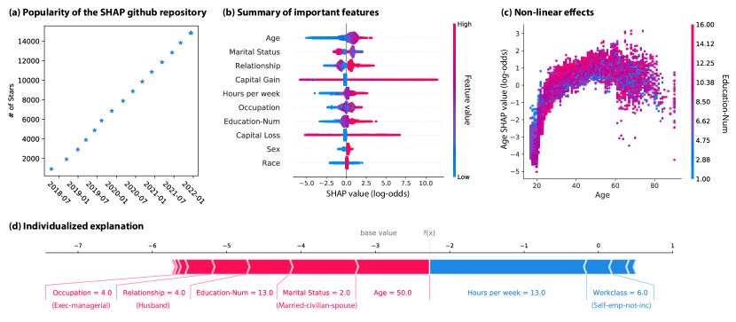
Figure 1: Shapley value explanations are popular and practical. (a) The large number of Github stars on shap (%feature␣attributionshttps://github.com/slundberg/shap), the most famous package to estimate Shapley value explanations, indicates their popularity. (b)-(d) A real-world example of Shapley value explanations for a tree ensemble model trained to predict whether individuals have income greater than 50,000 dollars based on census data. (b) Local feature attributions enable a global understanding of important features. (c) Local feature attributions help explain non-linear and interaction effects. (d) Local feature attributions explain how an individual’s features influence their outcome.

These two sources of complexity, properly removing features and accurately approximating Shapley values, have led to a wide variety of papers and algorithms on the subject. Unfortunately, this abundance of algorithms coupled with the inherent complexity of the topic have made the literature difficult to navigate, which can lead to misuse, especially given the popularity of Shapley value explanations (Figure 1a). To address this, we provide an approachable explanation of the sources of complexity underlying the computation of Shapley value explanations.

We discuss these difficulties in detail, beginning by introducing the preliminary concepts of feature attribution (Section 2) and the Shapley value (Section 3). Based on the various feature removal approaches, we then describe popular variants of Shapley value explanations as well as approaches to estimate the corresponding coalitional games (Section 4). Next, based on the estimation strategies, we describe model-agnostic and model-specific algorithms that rely on approximations and/or assumptions to tractably estimate Shapley value explanations (Section 5). These two sources of complexity provide a natural lens through which we present what is, to our knowledge, the first comprehensive survey of 24 distinct algorithms that combine different feature removal and tractable estimation strategies to compute Shapley value explanations. Finally, we identify gaps and important future directions in this area of research throughout the article.

2 Feature attributions

Given a model $f$ and features $x_{1},\ldots,x_{d}$, feature attributions explain predictions by assigning scalar values that represent each feature’s importance. For an intuitive description of feature attributions, we first consider linear models. Linear models of the form $f(x)=\beta_{0}+\beta_{1}x_{1}+\cdots+\beta_{d}x_{d}$ are often considered interpretable because each feature is linearly related to the prediction via a single parameter. In this case, a common global feature attribution that describes the model’s overall dependence on feature $i$ is the corresponding coefficient $\beta_{i}$. For linear models, each coefficient $\beta_{i}$ describes the influence that variations in feature $x_{i}$ have on the model output.

Alternatively, it may be preferable to give an individualized explanation that is not for the model as a whole, but rather for the prediction $f(x^{e})$ given a specific sample $x^{e}$. These types of explanations are known as local feature attributions, and the sample being explained ($x^{e}$) is called the explicand. For linear models, one reasonable local feature attribution is $\phi_{i}(f,x^{e})=\beta_{i}x^{e}_{i}$, because it is exactly the contribution that feature $i$ makes to the model’s prediction for the given explicand. However, note that this attribution hides within it an implicit assumption that we want to compare against an alternative feature value of $x_{i}=0$, but we may wish to account for other plausible alternative values, or more generally for the feature’s distribution or statistical relationships with other features (Section 4).

Linear models offer a simple case where we can understand each feature’s role via the model parameters, but this approach does not extend naturally to more complex model types. For model types that are most widely used today, including tree ensembles and deep learning models, their large number of operations prevents us from understanding each feature’s role by examining the model parameters. These flexible, non-linear models can capture more patterns in data, but they require us to develop more sophisticated and generalizable notions of feature importance. Thus, many researchers have recently begun turning to Shapley value explanations to summarize important features (Figure 1b), surface non-linear effects (Figure 1c), and provide individualized explanations (Figure 1d) in an axiomatic manner (Figure 2b).

3 Shapley values

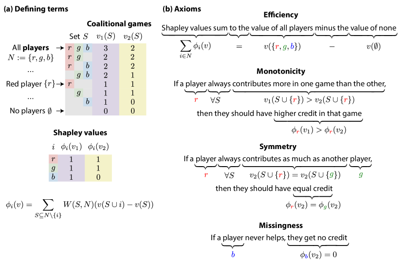
Figure 2: (a) Defining terms related to the Shapley value. Players either participate or abstain from the coalitional game, and the game maps from any subset of participating players to a scalar value. Shapley values are a solution concept to allocate credit to each player in a coalitional game. (b) A sufficient, but not exhaustive set of axioms that uniquely define the Shapley value.

Shapley values are a tool from game theory [35] designed to allocate credit to players in coalitional games. The players are represented by a set $D=\{1,\ldots,d\}$, and the coalitional game is a function that maps from subsets of the players to a scalar value. A game is represented by a subset function $v(S):\mathcal{P}(D)\mapsto\mathbb{R}$, where $\mathcal{P}(D)$ is the power set of $D$ (representing all possible subsets of players) (Figure 2a).

To make these concepts more concrete, we can imagine a company that makes a profit $v(S)$ determined by the set of employees $S\subseteq D$ that choose to work that day. A natural question is how to compensate the employees for their contribution to the total profit. Assuming we know the profit for all subsets of employees, Shapley values assign credit to an individual $i$ by calculating a weighted average of the profit increase when $i$ works with group $S$ versus when $i$ does not work with group $S$ (the marginal contribution). Averaging this difference over all possible subsets $S$ to which $i$ does not belong ($S\subseteq D\setminus\{i\}$), we arrive at the definition of the Shapley value:

$$\overbrace{\phi_{i}(v)}^{i\text{'s Shapley value}}=\sum_{S\subseteq D\setminus\{i\}}\underbrace{\frac{|S|!(|D|-|S|-1)!}{|D|!}}_{S\text{'s weight}}(\overbrace{v(S\cup\{i\})-v(S)}^{i\text{'s marginal contribution}})$$ (1)

Shapley values offer a compelling way to spread credit in coalitional games, and they have been widely adopted in fields including computational biology [36, 37], finance [38, 39], and more [40, 41]. Furthermore, they are a unique solution to the credit allocation problem as defined by several desirable properties [35, 42] (Figure 2b).

4 Shapley value explanations

In this section, we present common strategies to define local feature attributions based on the Shapley value. We also present intuitive examples based on explaining linear models, and we discuss the tradeoffs between various approaches to removing features.

4.1 Machine learning models are not coalitional games

Although Shapley values are an attractive solution for allocating credit among players in coalitional games, our goal is to allocate credit among features $x_{1},\ldots,x_{d}$ in a machine learning model $f(x)\in\mathbb{R}$. Machine learning models are not coalitional games by default, so to use Shapley values we must first define a coalitional game $v(S)$ based on the model $f(x)$ (Figure 3a). The coalitional game can be chosen to represent various model behaviors, including the model’s loss for a single sample or for the entire dataset [26], but our focus is the most common choice: explaining the prediction $f(x^{e})$ for a single sample $x^{e}$.

When explaining a machine learning model, it is natural to view each feature $x_{i}$ as a player in the coalitional game. However, we then must define what is meant by the presence or absence of each feature. Given our focus on a single explicand $x^{e}$, the presence of feature $i$ will mean that the model is evaluated with the observed value $x^{e}_{i}$ (Figure 3b). As for the absent features, we next consider how to remove them to properly assess the influence of the present features.

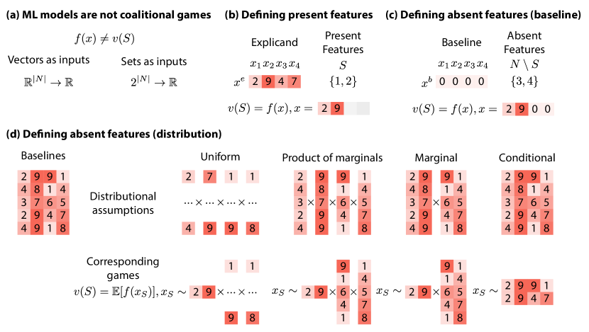
Figure 3: Empirical strategies for handling absent features. (a) Machine learning models have vector inputs and coalitional games have set inputs. For simplicity of notation we assume real-valued features, but Shapley value explanations can accommodate discrete features (unlike gradient-based methods). (b) Present features are replaced according to the explicand. (c) Absent features can be replaced according to a baseline. (d) Alternatively, absent features can be replaced according to a set of baselines with different distributional assumptions. In particular, the uniform approach uses the range of the baselines’ absent features to define independent uniform distributions to draw absent features from. The product of marginals approach draws each absent feature independently according to the values seen in the baselines. The marginal approach draws groups of absent feature values that appeared in the baselines. Finally, the conditional approach only considers samples that exactly match on the present features. Note that this figure depicts empirically estimating each expectation; however, in practice, the conditional approach is estimated by fitting models (Section 5.1.3).

4.2 Removing features with baseline values

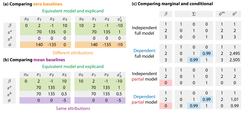
Figure 4: Shapley values for linear models. (a)-(b) A linear model ($\beta$), an explicand ($x^{e}$), a baseline ($x^{b}$), and baseline Shapley values ($\phi$) where feature 1 represents height (inches), feature 2 represents weight (lbs), and feature 3 represents gender. Features $x_{3}$ and $x_{3}^{\prime}$ denote different ways to represent gender, where $x_{3}=1$ is male and $x_{3}^{\prime}=1$ is female. (a) The models and explicands on the left and right are equivalent, but a zero baseline has a different meaning in each example and thus produces different attributions. (b) In this case, we use an mean baseline, for which the encoding of gender does not affect the baseline Shapley values. (c) Comparing marginal and conditional Shapley values for different models and feature dependencies with explicand $x^{e}=(1,1,1)$ and baseline $x^{b}=(0,0,0)$. Vectors $\beta$ (linear model coefficients), $\phi^{m}$ (marginal Shapley values), and $\phi^{c}$ (conditional Shapley values) have elements corresponding to $x_{1},x_{2},x_{3}$, and matrix $\Sigma$’s columns and rows are $x_{1},x_{2},x_{3}$. The independent models have no correlation between features and the dependent models have a surrogate feature (a highly correlated pair of features). The full model has all non-zero coefficients whereas the partial model has a zero coefficient for the third feature.

One straightforward way to remove a feature is to replace its value using a baseline sample $x^{b}$. That is, if a feature $i$ is absent, we simply set that feature’s value to be $x_{i}^{b}$. Then, the coalitional game is defined as $v(S)=f(\tau(x^{e},x^{b},S))$, where we define $\tau(x^{e},x^{b},S)_{i}=x^{e}_{i}\text{ if }i\in S$ or $x^{b}_{i}$ otherwise (Figure 3c). In words, we evaluate the model on a new sample where present features are the explicand values and absent features are the baseline values. As shorthand notation, we will refer to $f(\tau(x^{e},x^{b},S))$ as $f(x^{e}_{S},x^{b}_{\bar{S}})$ in the remainder of the paper.

The Shapley values for this coalitional game are referred to as baseline Shapley values [23]. This approach is simple to implement, but the choice of the baseline is not straightforward and can be somewhat arbitrary. Many different baselines have been considered, including an all-zeros baseline, an average across features, a baseline drawn from a uniform distribution, and more [20, 17, 43, 44, 45, 46]. Unfortunately, the choice of baseline heavily influences the feature attributions, and the criteria for choosing a baseline can be unclear. One possible motivation could be to find a neutral, uninformative baseline, but such a baseline value may not exist. For these reasons, it is common to use a distribution of baselines instead of relying on a single baseline.

4.3 Removing features with distributional values

Rather than setting the removed features to fixed baseline values, another option is to average the model’s prediction across randomly sampled replacement values; this may offer a better method to represent absent feature information. A first approach is to sample from the conditional distribution for the removed features. That is, given an explicand $x^{e}$ and subset $S\subseteq D$, we can consider the set of present features $x_{S}^{e}$ and then sample replacement values for the absent features according to $x_{\bar{S}}\sim p(x_{\bar{S}}\mid x_{S}^{e})$. In this case, the coalitional game is defined as the expectation of the prediction $f(x^{e}_{S},x_{\bar{S}})$ across this distribution. There are several names for Shapley values with this coalitional game: observational Shapley values [28], conditional expectation Shapley [23], and finally conditional Shapley values [25], which is how we will refer to them. Two issues with this approach are that estimating the conditional expectation is challenging (Section 5.1.3), and that the resulting explanations will spread credit among correlated features even if the model does not directly use all of them, which may not be desirable (Section 4.5).

An alternative approach is to use the marginal distribution when sampling replacement values. That is, we ignore the values for the observed features $x_{S}^{e}$ and sample replacement values according to $x_{\bar{S}}\sim p(x_{\bar{S}})$. As in the previous case, the coalitional game is defined as the expectation of the prediction across this distribution. This approach is equivalent to averaging over baseline Shapley values with baselines drawn from the data distribution $p(x)$ [23]. It also has an interpretation based in causal interventions on the feature values, but not interventions on the real-world values the features represent, interventions on the feature values in the computer going into the machine learning model. This is equivalent to assuming a flat causal graph (i.e., a causal graph with no causal links among features) [24, 25]. The latter interpretation has led to the name interventional Shapley values, but to avoid ambiguity we opt for the name marginal Shapley values [25].

The conditional and marginal approaches are by far the most common feature removal approaches in practice. Two other formulations based on random sampling are (1) the uniform approach, where absent features are drawn from a uniform distribution covering the feature range, and (2) the product of marginals approach, where absent features are drawn from their individual marginal distributions (which assumes independence between all absent features) [19, 47]. However, these distributions make a strong assumption of independence between all features, which may be why marginal Shapley values, which make a milder assumption of independence between the observed and unobserved features, are more commonly used. In addition, there are several other approaches for handling absent features in Shapley value-like explanations, but these can often be interpreted as approximations of the aforementioned approaches [26]. We visualized the three main removal approaches in Figure 3d, where, for simplicity, we show empirical versions that use a finite set of baselines (e.g., a training data set) to compute each expectation [23].

4.4 Shapley value explanations for linear models

To highlight intuitive differences between baseline, marginal, and conditional Shapley values, we consider the case of linear models where Shapley value explanations are easier to compute and compare (Figure 4). In the following examples, we consider different linear models, data distributions, and feature encodings to call attention to properties of these three types of Shapley value explanations.

Baseline Shapley values are simple and can be intuitive, but choosing an appropriate baseline is difficult. One common baseline is a sample with all zero feature values. However, we show that an all-zeros baseline can produce counterintuitive attribution values because the meaning of zero can be arbitrary (Figure 4a). In particular, we consider a case with equivalent models and explicand, but where the gender feature is encoded such that male is $0$ ($x_{3}$) or male is $1$ ($x_{3}^{\prime}$). In the first case, the baseline Shapley value for $x_{3}$ is zero (Figure 4a left), signaling that being male does not impact the prediction; however, in the second case, the baseline Shapley value for $x_{3}^{\prime}$ is $-10$ (Figure 4a right), suggesting that being male leads to lower predictions. These differing explanations are perhaps counterintuitive because the model and explicand are exactly equivalent, but the discrepancy arises because the meaning of zero is often arbitrary.

As an alternative to the all-zeros baseline, the mean baseline is arguably a reasonable choice for linear models. When using this baseline value, as in Figure 4b, the baseline Shapley value is zero for height and weight because the explicand’s height and weight are equal to their average values. In addition, for a mean baseline, the baseline Shapley value is the same regardless of how we encode gender. Although the mean baseline can work well for linear models (Section 5.2.3), it can be unappealing in other cases for two reasons. First, the mean of discrete features generally does not have a natural interpretation. For instance, the mean of the gender variable is half female and half male, a value that is never encountered in the dataset. This issue is compounded for non-ordinal discrete and categorical features with more than two possible values. Second, it may be impossible for any single baseline to represent the absence of feature information. For example, in images, removing features with a baseline cannot give credit to pixels that match the baseline [26, 44, 29]; for a mean baseline, this means that regions of images that resemble the mean will be biased towards lower importance.

Rather than baseline Shapley values, we may instead prefer to use marginal and conditional Shapley values, which we compare in Figure 4c. In this example, we compute Shapley value explanations for the same explicand and baseline, but with different models and data distributions (multivariate Gaussians with different covariances). We generate data in two ways: independent (zero covariance between features) or dependent (high covariance between features $x_{2}$ and $x_{3}$). In addition, we consider two models: full (all coefficients are non-zero) or partial ($\beta_{3}$ is zero).

Comparing the independent full model case to the dependent full model case, we can see that conditional Shapley values split credit between correlated features. This behavior may be desirable if we want to detect whether a model is relying on a protected class through correlated features. However, spreading credit can feel unnatural in the dependent partial model case, where the conditional Shapley value for feature $x_{3}$ ($\phi^{c}_{3}$) is as high as the conditional Shapley value for feature $x_{2}$ ($\phi^{c}_{2}$) even though feature $x_{3}$ is not explicitly used by the model ($\beta_{3}=0$). In particular, a common intuition is that features not algebraically used by the model should have zero attribution [23]. One concrete example is within a mortality prediction setting (NHANES; Appendix Section A.1.2), where [28] [28] show that for a model that does not explicitly use body mass index (BMI) as a feature, conditional Shapley values still give high importance to BMI due to correlations with other influential features such as arm circumference and systolic blood pressure.

4.5 Tradeoffs between removal approaches

Given the many ways to formulate the coalitional game, or to handle absent features, a natural question is which Shapley value explanation is preferred? This question is frequently debated in Shapley value literature, with some papers defending marginal Shapley values [23, 24], others advocating for conditional Shapley values [33, 49, 26], and still others arguing for causal solutions [25]. Before discussing differences, one way the approaches are alike is that each Shapley value explanation variant always satisfies the same axioms for its corresponding coalitional game, although the interpretation of the axioms can differ; this point has been discussed in prior work [23], but it is important to avoid conflating axioms defined relative to the coalitional game and relative to the model. Below, we discuss tradeoffs between the two most popular approaches, marginal and conditional Shapley values, because these are most commonly implemented in public repositories and discussed in the literature.

As we have seen with linear models, conditional Shapley values tend to spread credit between correlated features, which can surface hidden dependencies [50], whereas marginal Shapley values yield attributions that are a description of the model’s functional form [28]. This discrepancy arises from the distributional assumptions, where conditioning on a feature implicitly introduces information about all correlated features, thereby leading groups of correlated features to share credit (Figure 3 conditional). For example, if the feature weight is introduced when BMI is absent, then conditional Shapley values will only consider values of BMI that make sense given the known value of weight (i.e., “on-manifold” values); as a consequence, if the model depends on BMI but not weight, we would still observe that introducing weight affects the conditional expectation of the model output. In contrast, although marginal Shapley values perturb the data in less realistic ways (“off-manifold”), they are able to distinguish between correlated variables and identify whether the model functionally depends on BMI or weight, which is useful for model debugging [16].

Having two popular types of Shapley value explanations has been cited as a weakness [22], but this issue is not unique to Shapley values; it is encountered by a large number of model explanation methods [26], and it is fundamental to understanding feature importance with correlated or statistically dependent features. For example, with linear models, there are similar issues with handling correlation, where multicollinearity can result in different coefficients with equivalent accuracy. One solution to handle multicollinearity for linear models is to utilize appropriate regularization (e.g., ridge regression) [28], otherwise credit (coefficients) can be split among correlated features somewhat arbitrarily. In the model explanation context, correlated features represent a similar challenge, and the multiple ways of handling absent features can be understood as different approaches to disentangle credit for correlated features.

Another solution to address correlated features is to incorporate causal knowledge. Causal inference approaches typically assume knowledge of an underlying causal graph (i.e., a directed graph where edges indicate that one feature causes another) from which correlations between features arise. There are a number of Shapley value explanation methods that leverage an underlying causal graph, such as causal Shapley values [25], asymmetric Shapley values [51], and Shapley Flow [52]. The major drawback of these approaches is that they assume prior knowledge of causal graphs that are unknown in the vast majority of applications. For this reason, conditional and marginal Shapley values represent more viable options in many practical situations.

In this paper, we advocate for marginal and conditional Shapley values because they are more practical than causal Shapley values, and they avoid the problematic choice of a fixed baseline as in baseline Shapley values. In addition, they cover two of the most common use-cases for Shapley value explanations and model interpretation in general: (1) understanding a model’s informational dependencies, and (2) understanding the model’s functional form. An important final distinction between marginal and conditional Shapley values is the ease of estimation. As we discuss next in Section 5, marginal Shapley values turn out to be much simpler to estimate than conditional Shapley values.

5 Algorithms to estimate Shapley value explanations

Here, we describe algorithmic approaches to address the two main challenges for generating Shapley value explanations: (1) removing features to estimate the coalitional game, and (2) tractably calculating Shapley values despite their exponential complexity.

	Factors of complexity			Properties
Method	Estimation strategy	Removal approach	Removal variant	Model-agnostic	Bias-free	Variance-free
ApproSemivalue [30]	SV	None	Exact	Yes	Yes	No
L-Shapley [27]	SV	Marginal	Empirical	Yes	No	No♣
C-Shapley [27]	SV	Marginal	Empirical	Yes	No	No♣
ApproShapley [30]	RO	None	Exact	Yes	Yes	No
IME [21]	RO	Marginal	Empirical	Yes	Yes	No
CES [23]	RO	Conditional	Empirical	Yes	No	No
Shapley cohort refinement [53]	RO	Conditional	Empirical*	Yes	No	No
Generative model [50]	RO	Conditional	Generative	Yes	No	No
Surrogate model [50]	RO	Conditional	Surrogate	Yes	No	No
Multilinear extension sampling [31]	ME	Marginal	Empirical	Yes	Yes♢	No
SGD-Shapley [54]	WLS	Baseline	Exact	Yes	No♡	No
KernelSHAP [15, 55]	WLS	Marginal	Empirical	Yes	Yes♠	No
Parametric KernelSHAP [49]	WLS	Conditional	Parametric	Yes	No	No
Nonparameteric KernelSHAP [49]	WLS	Conditional	Empirical*	Yes	No	No
FastSHAP [32]	WLS	Conditional	Surrogate	Yes	No	No
LinearSHAP [28]	Linear	Marginal	Empirical	No	Yes	Yes
Correlated LinearSHAP [28]	Linear	Conditional	Parametric	No	No	No
Interventional TreeSHAP [16]	Tree	Marginal	Empirical	No	Yes	Yes
Path-dependent TreeSHAP [16]	Tree	Conditional	Empirical*	No	No	Yes
DeepLIFT [17]	Deep	Baseline	Exact	No	No	Yes
DeepSHAP [15]	Deep	Marginal	Empirical	No	No	Yes
DASP [33]	Deep	Baseline	Exact	No	No	No♣
Shallow ShapNet [34]	Deep	Baseline	Exact	No	Yes	Yes
Deep ShapNet [34]	Deep	Baseline	Exact	No	No	Yes

Table 1: Methods to estimate Shapley value explanations. We order approaches based on whether or not they are model-agnostic. Then, there are two factors of complexity. The first is the estimation strategy to handle the exponential complexity of Shapley values. For the model-agnostic approaches, the strategies include semivalue (SV), random order value (RO), multilinear extension (ME), and least squares value (LS). Note that the model-agnostic estimation strategies can generally be adapted to apply for any removal approach. For model-specific approaches, the strategies differ for linear, tree, and deep models. Then, the second factor of complexity is the feature removal approach which determines the type of Shapley value explanation (Section 5.1). “Any” denotes that it was introduced in game theory, and not for the sake of explaining a machine learning model. Then, we describe the specific removal variant employed by each algorithm. Baseline Shapley values are always computed exactly (Section 5.1.1), marginal Shapley values are always estimated empirically (Section 5.1.2), and conditional Shapley values have a variety of estimation procedures (Section 5.1.3). *These empirical estimates also involve defining a similarity metric. Finally, we report whether approaches are bias-free and/or variance-free. ^♢Multilinear extension sampling is unbiased when sampling $q$ uniformly. However, it is more common to use the trapezoid rule to determine $q$ which improves convergence, but can lead to higher bias empirically at smaller numbers of subsets (Appendix Tables 2, 3, 4). ^♡SGD-Shapley is consistent, but based on our empirical analysis it has high bias relative to other approaches (Appendix Tables 2, 3, 4). ^♠One version of KernelSHAP has been proven to be bias-free and the original version is asymptotically unbiased [56], although empirically it also appears to be unbiased for moderate numbers of samples [55]. ^♣These approaches can be deterministic with a polynomial number of model evaluations, but are often run with fewer evaluations for computational speed.

5.1 Feature removal approaches

Previously we introduced three main feature removal approaches and discussed tradeoffs between them. In this section, we discuss how to calculate the coalitional games that correspond to the most popular variants of Shapley value explanations: baseline Shapley values, marginal Shapley values, and conditional Shapley values.

5.1.1 Baseline Shapley values

The coalitional game for baseline Shapley values is defined as

$$v(S)=f(x^{e}_{S},x^{b}_{\bar{S}}),$$ (2)

where $f(x^{e}_{S},x^{b}_{\bar{S}})$ denotes evaluating $f$ on a hybrid sample where present features are taken from the explicand $x^{e}$ and absent features are taken from the baseline $x^{b}$. To compute the value of this coalitional game, we can simply create a hybrid sample and then return the model’s prediction for that sample. It is possible to exactly compute this coalitional game, unlike the remaining approaches. The only parameter is the choice of baseline, which can be a somewhat arbitrary decision.

5.1.2 Marginal Shapley values

For marginal Shapley values, the coalitional game is the marginal expectation of the model output,

$$v(S)=\mathbb{E}_{p(x_{\bar{S}})}[f(x^{e}_{S},x_{\bar{S}})],$$ (3)

where $x_{\bar{S}}$ is treated as a random variable representing the missing features and we take the expectation over the marginal distribution $p(x_{\bar{S}})$ for these missing features.

A natural approach to compute the marginal expectation is to leverage the training or test data to calculate an empirical estimate. A standard assumption in machine learning is that the data are independent draws from the data distribution $p(x)$, so we can designate a set of observed samples $E$ as an empirical distribution and use their values for the absent features (Figure 3d Marginal):

$$v(S)=\frac{1}{|E|}\sum_{x^{b}\in E}f(x^{e}_{S},x^{b}_{\bar{S}}).$$ (4)

From Eq. 4, it is clear that the empirical marginal expectation is the average over the coalitional games for baseline Shapley values with many baselines (Eq. 2). As a consequence, marginal Shapley values are also the average over many baseline Shapley values [29]. Due to this, some algorithms estimate marginal Shapley values by first estimating baseline Shapley values for many baselines and then averaging them [16, 29]. Note that marginal Shapley values based on empirical estimates are unbiased if the baselines are drawn i.i.d. from the baseline distribution (e.g., a random subset of rows from the dataset). As such, empirical estimates are considered a reliable way to approximate the true marginal expectation.

The empirical distribution can be the entire training dataset, but in practice it is often a moderate number of samples from the training or test data [23, 16]. The primary parameter is the number of baseline samples and how to choose them. If a large number of baselines is chosen, they can safely be chosen uniformly at random; however, when using a smaller number of samples, approaches based on k-means clustering can be used to ensure better coverage of the data distribution. This empirical approach also applies to other coalitional games such as the uniform and product of marginals, which are similarly easy to estimate [47].

5.1.3 Conditional Shapley values

For conditional Shapley values, the coalitional game is the conditional expectation of the model output,

$$v(S)=\mathbb{E}_{p(x_{\bar{S}}\mid x^{e}_{S})}[f(x^{e}_{S},x_{\bar{S}})],$$ (5)

where $x_{\bar{S}}$ is considered a random variable representing the missing features, and we take the expectation over the conditional distribution $p(x_{\bar{S}}\mid x^{e}_{S})$ of these missing features given the known features $x^{e}_{S}$ from the explicand.

Computing conditional Shapley values is more difficult because the required conditional distributions are not readily available from the training data. We can empirically estimate conditional expectations by averaging model predictions from samples that match the explicand’s present features (Figure 3d conditional), and this exactly estimates the conditional expectations as the number of baseline samples goes to infinity. However, this empirical estimate does not work well in practice: the number of matching rows may be too low in the presence of continuous features or a large number of features, leading to inaccurate and unreliable estimates [23]. For instance, if one conditions on a height of $5.879$ feet, there are likely very few individuals with that exact height, so the empirical conditional expectation will average over very few samples’ predictions, or potentially just the single prediction from the explicand itself.

One natural solution is to approximate the conditional expectation based on similar feature values rather than exact matches [53, 23, 49]. For instance, rather than condition on baselines that are $5.879$ feet tall, we can condition on baselines that are between $5.879\pm 0.025$ feet tall. This approach requires a definition of similarity, which is not obvious and may be an undesirable prerequisite for an explanation method. Furthermore, these approaches do not fully solve the curse of dimensionality, and conditioning on many features can still lead to inaccurate estimates of the conditional expectation.

Instead of empirical estimates, a number of approaches based on fitting models have been proposed to estimate the conditional expectations. Many of these have been identified in the broader context of removal-based explanations [26], but we reiterate them here, summarizing practical strengths and weaknesses:

• Parametric assumptions. [28] and [49] assume Gaussian or Gaussian-copula distributions. Conditional expectations for Gaussian random variables have closed-form solutions and are computationally efficient once the joint distribution’s parameters have been estimated, but these approaches can have large bias if the parametric assumptions are incorrect.

• Generative model. [50] use a conditional generative model to learn the conditional distributions given every subset of features. The generative model provides samples from approximate conditional distributions, and with these we can average model predictions to estimate the conditional expectation. In general, this approach is more flexible than simple parametric assumptions, but it has variance due to the stochastic nature of training deep generative models, and it is difficult to assess whether the generative model accurately approximates the exponential number of conditional distributions.

• Surrogate model. [50] use a surrogate model to learn the conditional expectation of the original model given every subset of features. The surrogate model is trained to match the original model’s predictions with arbitrarily held-out features, and doing so has been shown to directly approximate the conditional expectation, both for regression and classification models [26]. This approach is as flexible as the generative model, but it has several practical advantages: it is simpler to train, it requires only one model evaluation to estimate the conditional expectation, and it has been shown to provide a more accurate estimate in practice [50].

• Missingness during training. [26] describe an approach for directly estimating the conditional expectation by training the original model to accommodate missing features. Unlike the previous approaches, this approach cannot be applied post-hoc with arbitrary models because it requires modifying the training process.

• Separate models. [57], [58], and [56] directly estimate the conditional expectation given a subset of features as the output of a model trained with that feature subset. If every model is optimal (e.g., the Bayes classifier), then the conditional expectation estimate is exact [26]. In practice, however, the various models will be sub-optimal and unrelated to the original one, making it unsatisfying to view it as an explanation for the original model trained on all features. Furthermore, the computational demands of training models with many feature subsets is significant, particularly for non-linear models such as tree ensembles and neural networks.

As we have just shown, there are a wide variety of approaches to model conditional distributions or directly estimate the conditional expectations. These approaches will generally be biased, or inexact, because the coalitional game we require is based on the true underlying conditional expectation. Compounding this, it is difficult to quantify the approximation quality because the conditional expectations are unknown, except in very simple cases (e.g., synthetic multivariate Gaussian data).

Of these approaches, the empirical approach produces poor estimates, parametric approaches require strong assumptions, missingness during training is not model-agnostic, and separate models is not exactly an explanation of the original model. Instead, we believe approaches based on a generative model or a surrogate model are more promising. These approaches are more flexible, but both require fitting an additional deep model. To assess these deep models, [50] propose two reasonable metrics based on mean squared error of the model’s output to evaluate the generative and surrogate model approaches. Future work may include identifying robust architectures/hyperparameter optimization for surrogate and generative models, analyzing how conditional Shapley value estimates change for non-optimal surrogate and generative models, and evaluating bias in conditional Shapley value estimates for data with known conditional distributions.

Some of the approaches we discussed approximate the intermediate conditional distributions (empirical, parametric assumptions, generative model) whereas others directly approximate conditional expectations (surrogate model, missingness during training, separate models). It is worth noting that approaches based on modeling conditional distributions are independent of the particular model $f$. This suggests that if a researcher fits a high-quality generative model to a popular dataset, then any subsequent researchers can re-use this generative model to estimate conditional Shapley values for their own predictive models. However, even if fit properly, approaches based on modeling conditional distributions may be more computationally expensive, because they require evaluating the model with many generated samples to estimate the conditional expectation. As such, the surrogate model approach may be more effective than the generative model approach in practice [50], and it has been used successfully in recent work [32, 59].

In summary, in order to compute conditional Shapley values, there are two primary parameters: (1) the approach to model the conditional expectation, for which there are several choices. Furthermore, within the approaches that rely on deep models (generative model and surrogate model), the training and architecture of the deep model becomes an important yet complex dependency. (2) The baseline set used to estimate the conditional distribution or model the conditional expectation, because each approach requires a set of baselines (e.g., the training dataset) to learn dependencies between features. Different sets of baselines can lead to different scientific questions [47]. For instance, using baselines drawn from older male subpopulations, we can ask "why does an older male individual have a mortality risk of X% relative to the subpopulation of older males?" [29].

5.2 Tractable estimation strategies

Calculating Shapley values is, in the general case, an NP-hard problem [60, 61]. Intuitively, a brute force calculation based on Eq. 1 has exponential complexity in the number of features because it involves evaluating the model with all possible feature subsets. Given the long history of Shapley values, there is naturally considerable research into their calculation. Within the game theory literature, two types of estimation strategies have emerged [62, 63, 64]: (1) approximation-based strategies that produce unbiased Shapley value estimates for any game [30], and (2) assumption-based strategies that can produce exact results in polynomial time for specific types of games [65, 66, 30].

These two strategies have also prevailed in Shapley value explanation literature. However, because some approaches rely on both assumptions and approximations, we instead categorize the approaches as model-agnostic or model-specific. Model-agnostic estimation approaches make no assumptions on the model class and often rely on stochastic, sampling-based estimators [21, 15, 31, 32]. In contrast, model-specific approaches rely on assumptions about the machine learning model’s class to improve the speed of calculation, although sometimes at the expense of exactness [28, 16, 29, 33, 34].

5.2.1 Model-agnostic approaches

There are several types of model-agnostic approaches to estimate Shapley value explanations. In general, these are approximations that sidestep evaluating the model with an exponential number of subsets by instead using a smaller number of subsets chosen at random. These approaches are generally unbiased but stochastic; that is, their results are non-deterministic, but they are correct in expectation.

To introduce these approaches, we describe how each approximation can be tied to a distinct mathematical characterization of the Shapley value. We provided one such characterization in Section 3 (Eq. 1), but there are multiple equations to represent the Shapley value, and each one suggests its own approximation approach. For simplicity, we discuss these approaches in the context of a game $v$ where we ignore the choice of feature removal technique (baseline, marginal or conditional).

The classic Shapley value definition is as a semivalue [67], where each player’s credit is a weighted average of the player’s marginal contributions. For this we require a weighting function $P(S)$ that depends only on the subset’s cardinality, or where $\sum_{S\subseteq D\setminus\{i\}}P(S)=1$ for $i=1,\ldots,d$. Then, the value for player $i$ is given by

$$\phi_{i}(v)=\sum_{S\subseteq D\setminus\{i\}}P(S)\big{(}v(S\cup\{i\})-v(S)\big{)}.$$ (6)

[30] proposed an unbiased, stochastic estimator (ApproSemivalue) for any semivalue (i.e., with arbitrary weighting function) that involves sampling subsets from $D\setminus\{i\}$ with probability given by $P(S)$. In this algorithm, each player’s Shapley value is estimated one at a time, or independently. To use ApproSemivalue to estimate Shapley values, we simply have to draw subsets according to the distribution $P(S)=\frac{|S|!(|D|-|S|-1)!}{|D|!}$. While apparently simple, Shapley value estimators inspired directly by the semivalue characterization are uncommon in practice because sampling subsets from $P(S)$ is not straightforward.

Two related approaches are Local Shapley (L-Shapley) and Connected Shapley (C-Shapley) [27]. Unlike other model-agnostic approaches, L-Shapley and C-Shapley are designed for structured data (e.g., images) where nearby features are closely related (spatial correlation). Both approaches are biased Shapley value estimators because they restrict the game to consider only coalitions of players within the neighborhood of the player being explained. They are variance-free for sufficiently small neighborhoods, but for large neighborhoods it may still be necessary to use sampling-based approximations that introduce variance.

Next, the Shapley value can also be viewed as a random order value [35, 48], where a player’s credit is the average contribution across many possible orderings. Here, $\pi:\{1,\ldots,n\}\to\{1,\ldots,n\}$ denotes a permutation that maps from each position $j$ to the player $\pi(j)$. Then, $\Pi(D)$ denotes the set of all possible permutations and $Pre^{i}(\pi)$ denotes the set of predecessors of player $i$ in the order $\pi$ (i.e., $Pre^{i}(\pi)=\{\pi(1),\ldots,\pi(j-1)\}$, if $i=\pi(j)$). Then, the Shapley value’s random order characterization is the following:

$$\phi_{i}(v)=\frac{1}{|D|!}\sum_{\pi\subseteq\Pi(D)}(v(Pre^{i}(\pi)\cup\{i\})-v(Pre^{i}(\pi))).$$ (7)

There are two unbiased, stochastic estimation approaches based on this characterization. The first approach is IME (Interactions-based Method for Explanation) [21], which estimates Eq. 7 for each player with a fixed number of random permutations from $\Pi(D)$. Perhaps surprisingly, IME is analogous to ApproSemivalue, because identifying the preceding players in a random permutation can be understood as sampling from the probability distribution $P(S)$. One variant of IME improves the estimator’s convergence by allocating more samples to estimate $\phi_{i}(v)$ for players with high variance in their marginal contributions, which we refer to as adaptive sampling [68].

The second approach is ApproShapley, which explains all features simultaneously given a set of sampled permutations [30]. Rather than draw permutations independently for each player, this approach iteratively adds all players according to each sampled permutation so that all players’ estimates rely on the same number of marginal contributions based on the same permutations. There are many variants that aim to draw samples efficiently (i.e., reduce the variance of the estimates): antithetic sampling [69, 70], stratified sampling [71, 62], orthogonal spherical codes [70], and more [72, 70, 64]. Of these approaches, antithetic sampling is the simplest. After sampling a subset and evaluating its marginal contribution, antithetic sampling also evaluates the marginal contribution of the inverse of that subset ($N\setminus S$). Recent work finds that antithetic sampling provides near-best convergence in practice compared to several more complex methods [70].

The primary difference between IME and ApproShapley is that IME estimates $\phi_{i}(v)$ independently for each player, whereas ApproShapley estimates them simultaneously for $i=1,\ldots,d$. This means that IME can use adaptive sampling, which evaluates a different number of marginal contributions for each player and can greatly improve convergence when many players have low importance. In contrast, walking through permutations as in ApproShapley is advantageous because (1) it halves the number of evaluations of the game (which are expensive) by reusing them, and (2) it guarantees that the efficiency axiom is satisfied (i.e., the estimated Shapley values sum to the model’s prediction).

The third characterization of the Shapley value is as a least squares value [73, 74]. In this approach, the Shapley value is viewed as the solution to a weighted least squares (WLS) problem. The problem requires a weighting kernel $W(S)$, and the credits are the coefficients that minimize the following objective,

$$\phi(v)=\operatorname*{arg\,min}_{\beta}\sum_{S\subseteq D}W(S)(u(S)-v(S))^{2},$$ (8)

where $u(S)=\beta_{0}+\sum_{i\in S}\beta_{i}$ is an additive game. In order to obtain the Shapley value, we require the weighting kernel $W(S)=\frac{|D|-1}{{|D|\choose|S|}|S|(|D|-|S|)}$.

Based on this definition, a natural estimation approach is to sample a moderate number of subsets according to $W(S)$ and then solve the approximate WLS problem (Eq. 8). This approach is known as KernelSHAP [15], and its statistical properties have been studied in recent work: KernelSHAP is consistent and asymptotically unbiased [56], and it is empirically unbiased even for a moderate number of samples [55]. Variants of this approach include (1) a regularized version that introduces bias while reducing variance [15], and (2) an antithetic version that pairs each sampled subset with its complement to improve convergence [55].

Another approach that we refer to as SGD-Shapley is also based on the least squares characterization. It samples subsets according to the weighting kernel $W(S)$, but it iteratively estimates the solution from a random initialization using projected stochastic gradient descent [54]. Although it is possible to prove meaningful theoretical results for this strategy [54], our empirical evaluation shows that the KernelSHAP estimator consistently outperforms this approach in terms of its convergence (i.e., consistently lower estimation error given an equal number of samples) (Appendix Figures 6, 7, 8).

Finally, the last approach based on the least squares characterization is FastSHAP [32, 59]. FastSHAP learns a separate model (an explainer) to estimate Shapley values in a single forward pass, and it is trained by amortizing the WLS problem (Eq. 8) across many data examples. As a consequence of its WLS training objective, the globally optimal estimation model is a function that outputs exact Shapley values. Since the explanation model will generally be non-optimal, the resultant estimates offer imperfect accuracy and are random across separate training runs [32]. The major advantage of FastSHAP is that developers can frontload the cost of training the explanation model, thereby providing subsequent users with fast Shapley value explanations.

The fourth characterization of the Shapley value is based on a multilinear extension of the game [76, 31]. The multilinear extension extends a coalitional game to be a function on the $d$-cube $[0,1]^{d}$ that is linear separately in each variable. Based on an integral of the multilinear extension’s partial derivatives, the Shapley value can be defined as

$$\phi_{i}(v)=\int_{0}^{1}g_{i}(q)dq,$$ (9)

where $g_{i}(q)=\mathbb{E}[v(G_{i}\cup\{i\})-v(G_{i})]$ and $G_{i}$ is a random subset of $D\setminus\{i\}$, with each feature having probability $q$ of being included. Perhaps surprisingly, as with the random order value characterization, estimating this formulation involves averaging many marginal contributions where the subsets are effectively drawn from $P(S)=\frac{|S|!(|D|-|S|-1)!}{|D|!}$.

Based on this characterization, [31] introduced an unbiased sampling-based estimator that we refer to as multilinear extension sampling. The estimation consists of (1) sampling a $q$ from the range $[0,1]$, and then (2) sampling random subsets based on $q$ and evaluating the marginal contributions. This procedure introduces an additional parameter, which is the balance between the number of samples of $q$ and the number of subsets $E_{i}$ to generate for each value of $q$. The original version draws 2 random subsets for each $q$, where $q$ is sampled at fixed intervals according to the trapezoid rule [31]. Finally, in terms of variants, [31] find that antithetic sampling improves convergence, where for each subset they also compute the marginal contribution for the inverse subset.

To summarize, there are three main characterizations of the Shapley value from which unbiased, stochastic estimators have been derived: random order values, least squares values, and multilinear extensions. Within each approach, there are a number of variants. (1) Adaptive sampling, which has only been applied to IME (per-feature random order), but can easily be applied to a version of multilinear extension sampling that explains features independently. (2) Efficient sampling, which aims to carefully draw samples to improve convergence over independent sampling. In particular, one version of efficient sampling, antithetic sampling, is easy to implement and effective; it has been applied to ApproShapley, KernelSHAP, and multilinear extension sampling, and it can also be easily extended to IME. Although the other efficient sampling techniques have mainly been examined in the context of ApproShapley, similar benefits may exist for IME, KernelSHAP, and multilinear extension sampling. Finally, there is (3) amortized explanation models, which have only been applied to the least squares characterization [32], but may be extended to other characterizations that where the Shapley value can be viewed as the solution to an optimization problem.

5.2.2 Empirically comparing model-agnostic approaches

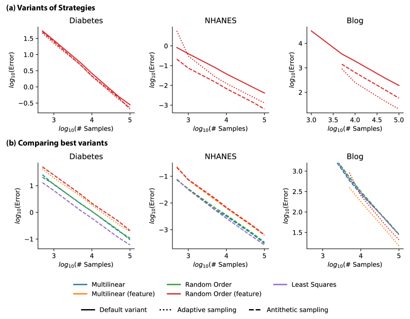
Figure 5: Benchmarking unbiased, model-agnostic algorithms to estimate baseline Shapley values for a single explicand and baseline on XGB models with 100 trees. For simplicity, we calculate baseline Shapley values for all methods because we aim to evaluate the tractable estimation strategy rather than the feature removal approach. In particular, the stochastic estimators include each sampling-based approach, where multilinear, random order, random order (feature), and least squares correspond to multilinear extension sampling [31], ApproShapley [30], IME [21], and KernelSHAP [15] respectively. Multilinear (feature) is a new approach based on the multilinear extension sampling approach which explains one feature at a time. In addition, some methods are variants: either antithetic or adaptive sampling. On the x-axis we report the number of samples (subsets) used for each estimate, and on the y-axis we report the MSE relative to the true baseline Shapley value for 100 estimates with that many samples. We use three real-world datasets: diabetes (10 features, regression), NHANES (79 features, classification), blog (280 features, regression). For some variants, no error is shown for small numbers of samples; this is because each approach requires a different minimum number of samples to produce estimates for each feature. (a) Variants of the random order, feature-wise strategy. We report the variants for all four strategies in Appendix Figures 6, 7, 8. (b) Benchmarking the most competitive variant of each stochastic estimator chosen according to the lowest error for $10^{5}$ samples. Note that the full blog error plot (Appendix Figure 9) is truncated to better showcase differences. Finally, the MSE can be decomposed into bias and variance terms [55], which we show in Appendix Tables 2, 3, 4, 5, 6, 7.

In Figure 5, we examine the convergence of the four main stochastic estimators (IME, ApproShapley, KernelSHAP and multilinear extension sampling) as well as several popular variants of these approaches (adaptive and antithetic sampling). We experiment with three datasets with varying numbers of features, all using XGBoost models. To calculate convergence, we calculate estimation error (mean squared error) of estimates of baselines Shapley values from the true baseline Shapley values computed using Interventional TreeSHAP. We also introduce four new approaches: IME with antithetic sampling, a new version of multilinear extension sampling that explain one feature at a time, and antithetic/adaptive sampling variants of this new multilinear extension sampling approach.

For the diabetes and NHANES datasets, which have 10 and 79 features respectively, the anthithetic version of KernelSHAP converges fastest to the true Shapley values. However, for the blog dataset, which has 280 features, we observe that IME and multilinear (feature) converge fastest, likely due to their use of adaptive sampling. Based on this finding, we hypothesize that adaptive sampling is important in the presence of many features, because with many features there are more likely to be features without interaction effects or with near-zero contributions. Such features will have little to no variance in their marginal contributions. We tested this hypothesis by modifying the diabetes dataset by adding 100 zero features that have no impact on the model and therefore no interaction effects. In this scenario, we find that the dummy features slow convergence and that the adaptive sampling approaches are least affected, likely because they can determine which features converge rapidly and then ignore them (Appendix Figures 10, 11).

Finally, an important desideratum of feature attribution estimates is the efficiency axiom [35], which means that the attributions sum to the game’s value with all players minus the value with none (Figure 2b). In terms of the sampling-based estimators, only ApproShapley and KernelSHAP are guaranteed to satisfy the efficiency property. However, it is possible to adjust attributions by evenly splitting the efficiency gap between all features using the additive efficient normalization operation [74]. This normalization step is used to ensure that the efficiency property holds for both FastSHAP and SGD-Shapley [32, 54]. It can also be used to ensure efficiency as a final post-processing step for IME and multilinear extension sampling, and it is guaranteed to improve estimates in terms of Euclidean distance to the true Shapley values without affecting the estimators’ bias [32].

These model-agnostic strategies for estimating Shapley values are appealing because they are flexible: they can be applied to any coalitional game and therefore any machine learning model. However, one major downside of these approaches is that they are inherently stochastic. Although most methods are guaranteed to be correct given an infinite number of samples (i.e., they are consistent estimators), users have finite computational budgets, leading to estimators with potentially non-trivial variance. In response, some methods utilize techniques to forecast and detect convergence when the estimated variance drops below a fixed threshold [77, 55]. However, even with convergence detection, model-agnostic explanations can be prohibitively expensive. Motivated in part by the computational complexity of these methods, a number of approaches have been developed to estimate Shapley value explanations more efficiently by making assumptions about the type of model being explained.

5.2.3 Model-specific approaches

In terms of model-specific approaches, algorithms have been designed for several popular model types: linear models, tree models, and deep models. These approaches are less flexible than model-agnostic approaches, in that they assume a specific model type and often a specific feature removal approach, but they are generally significantly faster to calculate.

First, one of the simplest model types to explain is linear models (also discussed in Section 4). For linear models, baseline and marginal Shapley values have a closed-form solution based on the coefficients of the linear model ($\beta$) and the values of the explicand ($x^{e}$) and the baseline(s). If we let $E$ represent a set of baseline values for marginal Shapley values, or $E=\{x^{b}\}$ for baseline Shapley values, we can write the mean value for feature $x_{i}$ as $\mu_{i}=\frac{1}{|E|}\sum_{x^{b}\in E}x^{b}$. Then, LinearSHAP [15, 68] gives the following result for the marginal or baseline Shapley values:

$$\phi_{i}(f,x^{e})=\beta_{i}(x^{e}_{i}-\mu^{b}_{i}).$$ (10)

Computing these values is straightforward, and it has linear complexity in the number of features, versus exponential complexity in the general case. Interestingly, for linear models the marginal Shapley value is equivalent to the baseline Shapley value with a mean baseline, which is why the mean baseline may be a good choice for linear models (see Section 4.4).

Alternatively, correlated LinearSHAP [28] estimates conditional Shapley values for linear models assuming that the data follows a multivariate Gaussian distribution. The key idea behind this approach is that for linear models, the expectation of the model’s prediction equals the model’s prediction for the average sample, or $\mathbb{E}[f(x)\mid x_{S}]=f(\mathbb{E}[x\mid x_{S}])$), which is not true in general. Using the closed-form solution for $\mathbb{E}[x\mid x_{S}]$ given multivariate normal data, we can calculate the conditional Shapley values as

$$\phi_{i}(f,x^{e})=\beta^{\top}A_{i}\mu+\beta^{\top}B_{i}x^{e},$$ (11)

where $\mu$ is the mean feature vector and $A_{i}$ and $B_{i}$ are summations over an exponential number of coalitions (see [28] for more details). In practice, $A_{i}$ and $B_{i}$ are estimated using a sampling-based procedure. Then, subsequent explanations are extremely fast to compute regardless of the explicand value. This approach resembles FastSHAP [32] because both approaches incur most of their computation up-front and then provide very fast explanations. Correlated LinearSHAP is biased if the data does not follow a multivariate Gaussian distribution, which is rarely the case in practice, and it is stochastic because $A_{i}$ and $B_{i}$ are estimated.

Next, another popular model type is tree models. Tree models include decision trees, as well as ensembles like random forests and gradient boosted trees. These are more complex than linear models and they can represent non-linear and interaction effects, but perhaps surprisingly, it is possible to calculate baseline and marginal Shapley values exactly (Interventional TreeSHAP) and approximate conditional Shapley values (Path-dependent TreeSHAP) tractably for such models.

Interventional TreeSHAP is an algorithm that exactly calculates baseline and marginal Shapley values in time linear in the size of the tree model and the number of baselines [16]. This is possible because a tree model can be represented as a disjoint set of outputs for each leaf in the tree. Then, each leaf’s contribution to any given feature’s Shapley value can be computed at the leaves of the tree assuming a coalitional game whose players are the features along the path from the root to the current leaf. Using a dynamic programming algorithm, Interventional TreeSHAP computes the Shapley value explanations for all features simultaneously by iterating through the nodes in the tree.

Then, Path-dependent TreeSHAP is an algorithm designed to estimate conditional Shapley values, where the conditional expectation is approximated by the structure of the tree model [16]. Given a set of present features, the algorithm handles internal nodes for absent features by traversing each branch in proportion to how many examples in the dataset follow each direction. This algorithm can be viewed as an application of Shapley cohort refinement [53], where the cohort is defined by the preceding nodes in the tree model and the baselines are the entire training set. In the end, it is possible to estimate a biased, variance-free version of conditional Shapley values in $O(LH^{2})$ time, where $L$ is the number of leaves and $H$ is the depth of the tree. Path-dependent TreeSHAP is a biased estimator for conditional Shapley values because its estimate of the conditional expectation is imperfect.

In comparison to Interventional TreeSHAP, Path-dependent TreeSHAP does not have a linear dependency on the number of baselines, because it utilizes node weights that represent the portion of baselines that fall on each node (based on the splits in the tree). Finally, in order to incorporate a tree ensemble, both approaches calculate explanations separately for each tree in the ensemble and then combine them linearly. This yields exact estimates for baseline and marginal Shapley values, because the Shapley value is additive with respect to the model [16].

Finally, another popular but opaque class of models are deep models (i.e., deep neural networks). Unlike for linear and tree models, we are unaware of any approach to estimate conditional Shapley values for deep models, but we discuss several approaches that estimate baseline and marginal Shapley values.

One early method to explain deep models, called DeepLIFT, was designed to propagate attributions through a deep network for a single explicand and baseline [17]. DeepLIFT propagates activation differences through each layer in the deep network, while maintaining the Shapley value’s efficiency property at each layer using a chain rule based on either a Rescale rule or a RevealCancel rule, which can be viewed as approximations of the Shapley value [29]. Due to the chain rule and these local approximations, DeepLIFT produces biased estimates of baseline Shapley values. Later, an extension of this method named DeepSHAP was designed to produce biased estimates of marginal Shapley values [29]. Despite its bias, DeepSHAP is useful because the computational complexity is on the order of the size of the model and the number of baselines, and the explanations have been shown to be useful empirically [78, 29]. In addition, the Rescale rule is general enough to propagate attributions through pipelines of linear, tree, and deep models [29].

Another method to estimate baseline Shapley values for deep models is Deep Approximate Shapley Propagation (DASP) [33]. DASP utilizes uncertainty propagation to estimate baseline Shapley values. To do so, the authors rely on a definition of the Shapley value that averages the expected marginal contribution for each coalition size. For each coalition size $k$ and a zero baseline, the input distribution from the random coalitions is modeled as a normal random variable whose parameters are a function of $k$. Since the input distributions are normal random variables, it is possible to propagate uncertainty for specific layers by matching first and second-order central moments and thereby estimate each expected marginal contribution. Based on an empirical study, DASP produces baseline Shapley values estimates with lower bias than DeepLIFT [33]. However, DASP is more computationally costly and requires up to $O(d^{2})$ model evaluations, where $d$ is the number of features. Although DASP is deterministic (variance-free) with $O(d^{2})$ model evaluations, it is biased because the moment propagation relies on an assumption of independent inputs that is violated at internal nodes whose inputs are given by the previous layer’s outputs.

One final method to estimate baseline Shapley values for deep models is Shapley Explanation Networks (ShapNets) [34]. ShapNets restrict the deep model to have a specific architecture for which baseline Shapley values are easier to estimate. The authors make a stronger assumption than DASP or DeepLIFT/DeepSHAP by not only restricting the model to be a neural network, but by requiring a specific architecture where hidden nodes have a small input dimension $h$ (typically between 2-4). In this setting, ShapNets can construct baseline Shapley values for each hidden node because the exponential cost is low for small $h$. The authors present two methods that follow the architecture assumption. (1) Shallow ShapNets: networks that have a single hidden layer, and where baseline Shapley values can be calculated exactly. Although they are easy to explain, these networks suffer in terms of model capacity and have lower predictive accuracy than other deep models. (2) Deep ShapNets: networks with multiple layers through which we can calculate explanations hierarchically. For Deep ShapNets, the final estimates are biased because of this hierarchical, layer-wise procedure. However, since Deep ShapNets can have multiple layers, they are more performant in terms of making predictions, although they are still more limited than standard deep models. An additional advantage of ShapNets is that they enable developers to regularize explanations based on prior information without a costly estimation procedure [34].

DASP and Deep ShapNets are originally designed to estimate baseline Shapley values with a zero baseline: DASP assumes a zero baseline to obtain an appropriate input distribution, and Deep ShapNets uses zero baselines in internal nodes. However, it may be possible to adapt DASP and Deep ShapNets to use arbitrary baselines (as in DeepLIFT and Shallow ShapNets), in which case it would be possible to estimate marginal Shapley values as DeepSHAP does. In terms of computational complexity, DeepLIFT, Shallow ShapNets, and Deep ShapNets can estimate baseline Shapley values with a constant number of model evaluations (for a fixed $h$). In contrast, DASP requires a minimum of $d$ model evaluations and up to $O(d^{2})$ model evaluations for a single estimate of baseline Shapley values.

A final difference between these approaches is in their assumptions. Shallow ShapNets and Deep ShapNets make the strongest assumptions by restricting the deep model’s architecture. DASP makes a strong assumption that we can perform first and second-order central moment matching for each layer in the deep model, and the original work only describes moment matching for affine transformations, ReLU activations and max pooling layers. Finally, DeepLIFT and DeepSHAP assume deep models, but they are flexible and support more types of layers than DASP or ShapNets. However, as a consequence of DeepLIFT’s flexibility, its baseline Shapley value estimates have higher bias compared to DASP or ShapNets [33, 34].

6 Discussion

In this work, we provided a detailed overview of numerous algorithms for generating Shapley value explanations. In particular, we delved into the two main factors of complexity underlying such explanations: the feature removal approach and the tractable estimation strategy. Disentangling the complexity in the literature into these two factors allows us to more easily understand the key innovations in recently proposed approaches.

In terms of feature removal approaches, algorithms that aim to estimate baseline Shapley values are generally unbiased, but choosing a single baseline to represent feature removal is challenging. Similarly, algorithms that aim to estimate marginal Shapley values will also generally be unbiased in their Shapley value estimates. Finally, algorithms that aim to estimate conditional Shapley values will be biased because the conditional expectation is fundamentally challenging to estimate. Conditional Shapley values are currently difficult to estimate with low bias and variance, except in the case of linear models; however, depending on the use case, it may be preferable to use an imperfect approximation rather than switch to baseline or marginal Shapley values.

In terms of the exponential complexity of Shapley values, model-agnostic approaches are often more flexible and bias-free, but they produce estimators with non-trivial variance. By contrast, model-specific approaches are typically deterministic and sometimes unbiased. Of the model-specific methods, only LinearSHAP and Interventional TreeSHAP have no bias for baseline and marginal Shapley values. In particular, we find that the Interventional TreeSHAP explanations are fairly remarkable for being non-trivial, bias-free, and variance-free. As such, tree models including decision trees, random forests, and gradient boosted trees are particularly well-suited to Shapley value explanations.

Furthermore, based on the feature removal approach and estimation strategy of each approach, we can understand the sources of bias and variance within many existing algorithms (Table 1). IME [21], for instance, is bias-free, because marginal Shapley values and the random order value estimation strategy are both bias-free. However, IME estimates have non-zero variance because the estimation strategy is stochastic (random order value sampling). In contrast, Shapley cohort refinement estimates [53] have both non-zero bias and non-zero variance. Their bias comes from modeling the conditional expectation using an empirical, similarity-based approach, and the variance comes from the sampling-based estimation strategy (random order value sampling).

In practice, Shapley value explanations are widely used in both industry and academia. Although they are powerful tools for explaining models, it is important for users to be aware of important parameters associated with the algorithms used to estimate them. In particular, we recommend that any analysis based on Shapley values should report parameters including the type of Shapley value explanation (the feature removal approach), the baseline distribution used to estimate the coalitional game, and the estimation strategy. For sampling-based strategies, it is important for users to include a discussion of convergence in order to validate their feature attribution estimates. Finally, developers of Shapley value explanation tools should strive to be transparent about convergence by explicitly performing automatic convergence detection. Convergence results based on the central limit theorem are straightforward for the majority of model-agnostic estimators we discussed, although they are not always implemented in public packages. Note that convergence analysis is more difficult for the least squares estimators, but [55] discuss this issue and present a convergence detection approach for KernelSHAP.

Future research directions include investigating new stopping conditions for convergence detection. Existing work proposes stopping once the largest standard deviation is smaller than a prescribed threshold [55], but depending on the threshold, the variance may still be high enough that the relative importance of features can change. Therefore, a new stopping condition could be when additional marginal contributions are highly unlikely to change the relative ordering of attributions for all features. Another important future research direction is Shapley value estimation for deep models. Current model-specific approaches to explain deep models are biased, even for marginal Shapley values, and no model-specific algorithms exist to estimate conditional Shapley values. One promising model-agnostic approach is FastSHAP [32, 59], which speeds up explanations using an explainer model, although it requires a large upfront cost to train this model. Finally, because approximating the conditional expectation for conditional Shapley values is so hard, it constitutes an important future research direction that would benefit from new methods or systematic evaluations of existing approaches.

7 Recommendations based on data domain

What we have discussed in this paper is largely agnostic to the type of data. However, there are a few characteristics of the data being analyzed that may change the best practices for generating Shapley value explanations.

The first characteristic is the number of features. Models with more input features will be more computationally expensive to explain. In particular, for model-agnostic algorithms, as the number of features increases, the total number of possible coalitions increases exponentially. In this setting it may be valuable to reduce the number of features by carefully filtering the ones which do not vary or are highly redundant with other features. This type of feature selection can even be performed prior to model-fitting and is already a common practice.

The second characteristic is the number of samples. The number of samples likely plays a larger role in fitting the original predictive model than in generating the explanation. However, for conditional Shapley values, having a large number of samples is important for creating accurate estimates of the conditional expectations/distributions. If the number of samples is very low, it may be better to rely on parametric assumptions or use marginal Shapley values instead.

The third characteristic is the feature correlation. In highly correlated settings, one can expect larger discrepancies between marginal and conditional Shapley values. Then, carefully choosing the feature removal approach or comparing estimates of both marginal and conditional Shapley values can be valuable. Highly correlated features can also make it harder to understand feature attributions in general. For images in particular, the importance of a single pixel may not be semantically meaningful in isolation. In these cases, it may be useful to use explanation methods that aim to understand higher level concepts [79].

Beyond correlated features, there may also be structure within the data. Tabular data are typically considered unstructured whereas image and text data is structured because neighboring pixels and words are strongly correlated. For tabular data, it may be best to use tree ensembles (gradient boosted trees or random forests) which are both performant and easy to explain using the two versions fo TreeSHAP (Interventional and Path-dependent) [16]. For structured data, it may be valuable to use methods such as L-Shapley and C-Shapley that are designed to estimate Shapley value explanations more tractably in structured settings [27]. Furthermore, grouping features may be natural for structured data (e.g., superpixels for image data or sentences/n-grams for text data), because it greatly reduces the computational complexity of most algorithms. Finally, since structured data often calls for complex deep models, which are expensive to evaluate, methodologies such as FastSHAP can be useful for accelerating explanations.

The fourth characteristic is prior knowledge of causal relationships. Although causal knowledge is unavailable for the vast majority of datasets, it can be used to generate Shapley value explanations that better respect causal relationships [25, 51] or generate explanations that assign importance to edges in the causal graph [52]. These techniques may be a better alternative to conditional Shapley values, which respect the data manifold, because they respect the causal relationships underlying the correlated features.

The fifth characteristic is whether there is a natural interpretation of absent features. For certain types of data, there may be preconceived notions of feature absence. For instance, in text data it may be natural to remove features from models that take variable length inputs or use masking tokens to denote feature removal. In images, it is often common to assume some form of gray, black, or blurred baseline; these approaches are somewhat dissatisfying because they are data-specific notions of feature removal. However, given that model evaluations are often exorbitantly expensive in these domains, these techniques may provide simple, yet tractable alternatives to marginal or conditional Shapley values.

8 Related work

In this paper, we focused on describing popular algorithms to estimate local feature attributions based on the Shapley value. However, there are a number of adjacent explanation approaches that are not the focus of this discussion. Two broad categories of such approaches include alternative definitions of coalitional games, and different game-theoretic solution concepts.

We focus on three popular coalitional games where the players represent features and the value is the model’s prediction for a single example. However, as discussed by [26], there are several methods that use different coalitional games, including global feature attributions where the value is the model’s mean test loss [77], and local feature attributions where the value is the model’s per-sample loss [16]. Other examples include games where the value is the maximum flow of attention weights in transformer models [80], where the players are analogous to samples in the training data [81], where the players are analogous to neurons in a deep model [82], and where the players are analogous to edges in a causal graph [52]. Although these methods are largely outside the scope of this paper, a variety of applications of the Shapley value in machine learning are discussed in [83].

Secondly, there are game-theoretic solution concepts beyond the Shapley value that can be utilized to explain machine learning models. The first method, named asymmetric Shapley values, is designed to generate feature attributions that incorporate causal information [51]. To do so, asymmetric Shapley values are based on random order values where weights are set to zero if they are inconsistent with the underlying causal graph. Next, L-Shapley and C-Shapley (also discussed in Section 5.2.1) are computationally efficient estimators for Shapley value explanations designed for structured data; they are technically probabilistic values, a generalization of semivalues [27, 48]. Similarly, Banzhaf values, an alternative to Shapley values, are also semivalues, but each coalition is given equal weight in the summation (see Eq. 1). Banzhaf values have been used to explain machine learning models in a variety of settings [84, 85]. Another solution concept designed to incorporate structural information about coalitions is the Owen value. The Owen value has been used to design a hierarchical explanation technique named PartitionExplainer within the SHAP package and as a way to accommodate groups of strongly correlated features [86]. Finally, Aumann-Shapley values are an extension of Shapley values to infinite games [87], and they are connected to an explanation method named Integrated Gradients [20]. Integrated Gradients requires gradients of model’s prediction with respect to the features, so it cannot be used for certain types of non-differentiable models (e.g., tree models, nearest neighbor models), and it represents features’ absence in a continuous rather than discrete manner that typically requires a fixed baseline (similar to baseline Shapley values).

Data and code availability

The diabetes dataset is publicly available (https://www4.stat.ncsu.edu/~boos/var.select/diabetes.html), and we use the version from the sklearn package. The NHANES dataset is publicly available (https://wwwn.cdc.gov/nchs/nhanes/nhefs/), and we use the version from the shap package. The blog dataset is publicly available (https://archive.ics.uci.edu/ml/datasets/BlogFeedback).

Code availability

The code for the experiments is available here: https://github.com/suinleelab/shapley_algorithms.

Appendix A Appendix

A.1 Datasets

In order to compare the unbiased stochastic estimators and their variants, we utilize three datasets with varying numbers of features.

A.1.1 Diabetes

The diabetes dataset ($n=442$) consists of ten input features (e.g., age, sex, BMI, etc.) and a continuous output which is diabetes disease progression measured one year after measuring baseline features.

A.1.2 NHANES

The NHANES (National Health and Nutrition Examination Survey) (I) dataset ($n=14264$) consists of 79 input features (e.g., age, sex, BMI, etc.) and a binary output for which the positive label is 5-year mortality after measuring the patient features.

A.1.3 Blog

The blog dataset ($n=52397$) consists of 280 features (e.g., number of comments, length of blog post, etc.) and a non-binary output which is the number of comments in the next twenty-four hours.

A.2 Experiments

In Figures 6-11, we show more comprehensive comparisons of the various estimators’ error based on mean squared error between estimated baseline Shapley values and the true baseline Shapley values estimated by TreeSHAP. See Figure 5 for a description of each method. We include two new variants: “Random q” is multilinear extension sampling with uniformly drawn $q$ and “Stochastic Gradient Descent” is SGD-Shapley [54], which is only applicable to the least squares estimator. Note that missing values denote that we had insufficient numbers of samples (coalitions) to create an estimate of the feature attribution for all features.

In Tables 2-7, we show the bias and variance of each approach, which sum to the estimator error [55]. We refer to the estimators using shorthand in the tables. In particular, the stochastic estimators include each sampling-based approach, where the prefixes MEF (multilinear extension, feature-wise), ROF (random order, feature-wise), RO (random order), and LS (least squares) correspond to multilinear extension sampling [31], IME [21], ApproShapley [30], and KernelSHAP [15] respectively. The suffixes “ANTI” and “ADAPT” stand for antithetic sampling and adaptive sampling respectively. Finally, “SGD” is SGD-Shapley and “RAND” is multilinear extension sampling with uniformly drawn $q$.

These results largely mirror the results in Figure 5. Antithetic and adaptive sampling are largely helpful. In the diabetes dataset, which has a small number of features, antithetic and adaptive sampling are only mildly helpful. For NHANES, which has a medium number of features, there is a larger separation between approaches and antithetic sampling is more helpful than adaptive sampling. For the blog dataset, which has a large number of features, adaptive sampling is more beneficial than antithetic sampling. For the multilinear approaches, we find that using a random $q$ naturally produces results very similar to the random order sampling approaches. This is natural because they are actually equivalent approaches to sampling subsets from the appropriate distribution $P(S)$. However, we do see that the default version of multilinear sampling benefits over random $q$ by sampling $q$ at fixed intervals according to the trapezoid rule. Finally, we see that for the least squares estimators, using SGD is unhelpful. Note that some approaches have non-zero bias although they are provably unbiased. This is because of the number of trials performed. If we performed more trials, their bias would continue to shrink.

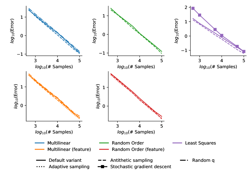
Figure 6: Errors for all variants of unbiased stochastic estimators in the diabetes dataset.

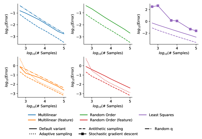
Figure 7: Errors for all variants of unbiased stochastic estimators in the NHANES dataset.

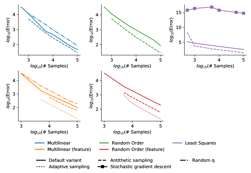
Figure 8: Errors for all variants of unbiased stochastic estimators in the blog dataset.

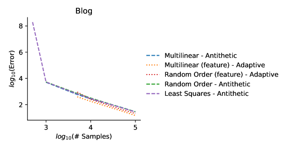
Figure 9: Untruncated comparison of best variants on the blog dataset.

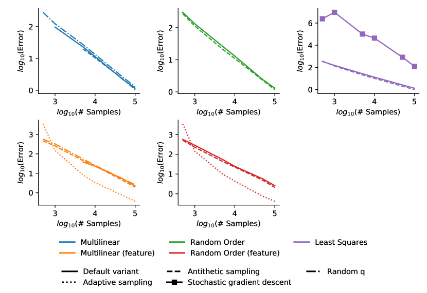
Figure 10: Errors for all variants of unbiased stochastic estimators in the diabetes dataset (with 100 additional zero features).

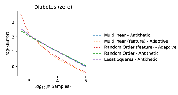
Figure 11: Comparison of best variants in the diabetes dataset with 100 additional zero features.

	500	1000	5000	10000	50000	100000
ME	1.03307	0.10672	0.00882	0.01493	0.0019	0.00103
ME_RAND	0.14194	0.16995	0.03135	0.01725	0.00251	0.00062
ME_ANTI	2.20398	0.61293	0.0586	0.03112	0.00139	0.00072
MEF	1.1593	0.93785	0.04937	0.01506	0.00507	0.00246
MEF_RAND	0.31587	0.21718	0.01556	0.0228	0.0015	0.00604
MEF_ADAPT	8.92679	1.18728	0.13272	0.03672	0.0013	0.00155
MEF_ANTI	10.47164	2.51886	0.13555	0.03785	0.00179	0.00254
RO	0.25328	0.13665	0.04269	0.00863	0.00248	0.00268
RO_ANTI	0.07361	0.16267	0.01586	0.01166	0.00082	0.00059
ROF	0.15102	0.22011	0.03267	0.047	0.00572	0.00221
ROF_ADAPT	0.46465	0.22019	0.05365	0.01299	0.00403	0.00348
ROF_ANTI	0.47356	0.21328	0.01301	0.01196	0.00784	0.00207
LS	0.29439	0.06221	0.00499	0.00546	0.00323	0.00047
LS_ANTI	0.18394	0.15229	0.00925	0.00485	0.00255	0.00062
LS_SGD	43.17269	13.02032	0.50849	0.116	0.00464	0.00135

Table 2: Biases in the diabetes dataset.

	500	1000	5000	10000	50000	100000
ME	0.01634	0.00219	0.0002	0.00026	3e-05	4e-05
ME_RAND	0.00337	0.00371	0.00031	0.00025	7e-05	2e-05
ME_ANTI	0.00061	0.01537	0.00019	8e-05	1e-05	0.0
MEF	0.00686	0.01644	0.00051	0.0003	3e-05	2e-05
MEF_RAND	0.00444	0.00152	0.00035	0.00037	7e-05	3e-05
MEF_ADAPT		0.00611	0.00076	0.0002	1e-05	1e-05
MEF_ANTI	0.00248	0.00041	0.00146	0.00029	2e-05	0.0
RO	0.00096	0.00196	0.00014	0.00013	2e-05	1e-05
RO_ANTI	0.00041	0.00016	0.0001	1e-05	0.0	0.0
ROF	0.00396	0.0044	0.00054	0.0004	8e-05	2e-05
ROF_ADAPT		0.00516	0.00013	0.00015	3e-05	1e-05
ROF_ANTI	0.003	0.00047	0.00012	7e-05	1e-05	0.0
LS	0.00441	0.00193	0.00032	0.00022	3e-05	2e-05
LS_ANTI	0.00188	0.00039	5e-05	2e-05	0.0	0.0
LS_SGD	2.40455	4.0216	0.00907	0.00703	0.00045	0.00019

Table 3: Biases in the NHANES dataset.

	500	1000	5000	10000	50000	100000
ME	338.01236	178.15781	144.77503	13.6816	1.86531	0.59309
ME_RAND	610.90174	99.46345	24.6845	17.25537	6.09554	1.5173
ME_ANTI		83.27304	573.95994	89.70199	1.58388	0.80663
MEF		395.61402	592.00777	69.757	11.14579	4.95535
MEF_RAND		486.29512	113.96514	35.53342	2.63154	7.78507
MEF_ADAPT			719.24301	108.48492	5.07824	0.71839
MEF_ANTI				555.99106	10.3927	3.22064
RO	811.14593	360.14181	142.15739	45.46918	5.03847	2.11807
RO_ANTI		268.88612	20.02851	4.23618	2.26818	0.74835
ROF		941.03632	66.14242	24.57762	13.38569	2.99248
ROF_ADAPT			79.202	23.71196	1.32897	0.94973
ROF_ANTI			29.90393	13.26942	1.75937	0.58583
LS	5140.67576	1640.50381	207.70321	116.66386	20.67612	10.15152
LS_ANTI	5589054.21794	525.46966	29.46567	10.70906	1.70923	0.78873
LS_SGD	1.4363e+14	6.1849e+14	1.8168e+15	1.5086e+14	2.9198e+13	1.4884e+13

Table 4: Biases in the blog dataset.

	500	1000	5000	10000	50000	100000
ME	22.96666	12.07279	2.5081	1.37924	0.2432	0.11547
ME_RAND	29.62088	14.31613	2.89015	1.44624	0.28177	0.13646
ME_ANTI	23.43875	10.42177	2.09982	1.06178	0.19789	0.10684
MEF	41.77143	20.47749	4.35186	2.41331	0.38869	0.21297
MEF_RAND	50.69169	23.15461	4.82135	2.58893	0.44981	0.25554
MEF_ADAPT	34.51499	18.23867	3.99338	1.86179	0.35407	0.18755
MEF_ANTI	32.8124	16.97314	3.63817	1.9772	0.42555	0.19555
RO	24.84541	11.66307	2.63066	1.13767	0.24184	0.1187
RO_ANTI	20.58076	11.24632	2.09441	1.07522	0.21244	0.09355
ROF	53.78942	27.42756	5.58406	2.5637	0.5001	0.27848
ROF_ADAPT	45.63946	21.95396	4.75253	2.10057	0.41285	0.22687
ROF_ANTI	50.41685	24.72881	4.7859	2.1644	0.45592	0.205
LS	16.28934	7.47362	1.5866	0.78921	0.16094	0.08113
LS_ANTI	12.98929	6.39006	1.16766	0.59549	0.11076	0.0598
LS_SGD	41.51592	15.59966	2.33451	0.97674	0.1831	0.08241

Table 5: Variances in the diabetes dataset.

	500	1000	5000	10000	50000	100000
ME	0.10806	0.07575	0.02124	0.01065	0.00206	0.00129
ME_RAND	0.33544	0.15789	0.02918	0.01401	0.00282	0.00154
ME_ANTI	0.05972	0.01036	0.00433	0.00244	0.00051	0.00024
MEF	0.59095	0.10908	0.04178	0.02123	0.00447	0.00187
MEF_RAND	0.62686	0.32213	0.06354	0.03194	0.00598	0.00325
MEF_ADAPT		0.22775	0.01328	0.0069	0.00149	0.00068
MEF_ANTI	0.17626	0.05679	0.00915	0.00481	0.00101	0.00049
RO	0.30973	0.16971	0.03165	0.01606	0.00345	0.00163
RO_ANTI	0.05721	0.02674	0.00511	0.00278	0.00057	0.00027
ROF	0.64611	0.31183	0.06334	0.02974	0.00625	0.00323
ROF_ADAPT		0.23807	0.0216	0.00981	0.00198	0.00102
ROF_ANTI	0.16582	0.05885	0.01168	0.00532	0.00109	0.00051
LS	0.41585	0.19099	0.03514	0.01713	0.00339	0.00165
LS_ANTI	0.05979	0.02459	0.0043	0.00209	0.00042	0.00021
LS_SGD	247.45077	361.76017	1.1384	0.9365	0.03746	0.01957

Table 6: Variances in the NHANES dataset.

	500	1000	5000	10000	50000	100000
ME	86410.36336	30866.41722	1997.75462	1281.98781	227.58978	129.44555
ME_RAND	84274.19531	31874.46777	5954.03044	2590.77554	493.77726	226.55744
ME_ANTI		14121.88171	1076.49978	680.50752	166.27577	78.60651
MEF		89335.0449	4330.56682	2375.37671	542.53634	264.14241
MEF_RAND		96454.13874	10778.75215	5232.66527	873.32245	537.40648
MEF_ADAPT			385.15507	391.50072	85.38466	40.68452
MEF_ANTI				1071.56372	284.39153	164.1287
RO	90722.92558	31639.72416	5028.47504	2659.61346	596.35393	245.73287
RO_ANTI		14649.27372	1965.69685	886.23589	159.37583	79.43453
ROF		89654.02281	10234.68309	5268.76653	1020.95547	534.06821
ROF_ADAPT			2479.70421	679.7336	115.98881	57.75736
ROF_ANTI			3914.76444	1797.94149	339.38264	162.71561
LS	3.9848e5	1.4281e5	22220.79433	10600.85713	2062.52593	1032.15956
LS_ANTI	5.4101e+8	14374.92093	1777.1319	819.92753	157.75298	76.68178
LS_SGD	1.5715e+16	5.9717e+16	1.7423e+17	1.5233e+16	3.0639e+15	1.4746e+14

Table 7: Variances in the blog dataset.

References

- [1] David Silver et al. “Mastering the game of Go without human knowledge” In Nature 550.7676 Nature Publishing Group, 2017, pp. 354–359
- [2] Matej Moravcik et al. “Deepstack: Expert-level artificial intelligence in heads-up no-limit poker” In Science 356.6337 American Association for the Advancement of Science, 2017, pp. 508–513
- [3] Oriol Vinyals et al. “Grandmaster level in StarCraft II using multi-agent reinforcement learning” In Nature 575.7782 Nature Publishing Group, 2019, pp. 350–354
- [4] John Jumper et al. “Highly accurate protein structure prediction with AlphaFold” In Nature 596.7873 Nature Publishing Group, 2021, pp. 583–589
- [5] Sebastien Jean, Kyunghyun Cho, Roland Memisevic and Yoshua Bengio “On using very large target vocabulary for neural machine translation” In arXiv preprint arXiv:1412.2007, 2014
- [6] Leo Breiman “Random forests” In Machine Learning 45.1 Springer, 2001, pp. 5–32
- [7] Yann LeCun, Yoshua Bengio and Geoffrey Hinton “Deep learning” In Nature 521.7553 Nature Publishing Group, 2015, pp. 436–444
- [8] Tianqi Chen and Carlos Guestrin “XGBoost: A scalable tree boosting system” In Proceedings of the 22nd ACM SIGKDD International Conference on Knowledge Discovery and Data Mining, 2016, pp. 785–794
- [9] Dave Steinkraus, Ian Buck and PY Simard “Using GPUs for machine learning algorithms” In Eighth International Conference on Document Analysis and Recognition (ICDAR’05), 2005, pp. 1115–1120 IEEE
- [10] Robert Geirhos et al. “Shortcut learning in deep neural networks” In Nature Machine Intelligence 2.11 Nature Publishing Group, 2020, pp. 665–673
- [11] Finale Doshi-Velez and Been Kim “Towards a rigorous science of interpretable machine learning” In arXiv preprint arXiv:1702.08608, 2017
- [12] Andrew Selbst and Julia Powles ““Meaningful Information” and the Right to Explanation” In Conference on Fairness, Accountability and Transparency, 2018, pp. 48–48 PMLR
- [13] Eric Knight “AI and Machine Learning-Based Credit Underwriting and Adverse Action under the ECOA” In Bus. & Fin. L. Rev. 3 HeinOnline, 2019, pp. 236
- [14] Marco Tulio Ribeiro, Sameer Singh and Carlos Guestrin “" Why should I trust you?" Explaining the predictions of any classifier” In Proceedings of the 22nd ACM SIGKDD International Conference on Knowledge Discovery and Data Mining, 2016, pp. 1135–1144
- [15] Scott M Lundberg and Su-In Lee “A unified approach to interpreting model predictions” In Advances in Neural Information Processing Systems, 2017, pp. 4765–4774
- [16] Scott M Lundberg et al. “From local explanations to global understanding with explainable AI for trees” In Nature Machine Intelligence 2.1, 2020, pp. 56–67
- [17] Avanti Shrikumar, Peyton Greenside and Anshul Kundaje “Learning important features through propagating activation differences” In Proceedings of the 34th International Conference on Machine Learning-Volume 70, 2017, pp. 3145–3153 JMLR. org
- [18] Alexander Binder et al. “Layer-wise relevance propagation for neural networks with local renormalization layers” In International Conference on Artificial Neural Networks, 2016, pp. 63–71 Springer
- [19] Anupam Datta, Shayak Sen and Yair Zick “Algorithmic transparency via quantitative input influence: Theory and experiments with learning systems” In 2016 IEEE Symposium on Security and Privacy (SP), 2016, pp. 598–617 IEEE
- [20] Mukund Sundararajan, Ankur Taly and Qiqi Yan “Axiomatic attribution for deep networks” In International Conference on Machine Learning, 2017, pp. 3319–3328 PMLR
- [21] Erik Strumbelj and Igor Kononenko “An efficient explanation of individual classifications using game theory” In The Journal of Machine Learning Research 11 JMLR. org, 2010, pp. 1–18
- [22] I Elizabeth Kumar, Suresh Venkatasubramanian, Carlos Scheidegger and Sorelle Friedler “Problems with Shapley-value-based explanations as feature importance measures” In International Conference on Machine Learning, 2020, pp. 5491–5500 PMLR
- [23] Mukund Sundararajan and Amir Najmi “The many Shapley values for model explanation” In International Conference on Machine Learning, 2020, pp. 9269–9278 PMLR
- [24] Dominik Janzing, Lenon Minorics and Patrick Blobaum “Feature relevance quantification in explainable AI: A causal problem” In International Conference on Artificial Intelligence and Statistics, 2020, pp. 2907–2916 PMLR
- [25] Tom Heskes, Evi Sijben, Ioan Gabriel Bucur and Tom Claassen “Causal Shapley values: Exploiting causal knowledge to explain individual predictions of complex models” In arXiv preprint arXiv:2011.01625, 2020
- [26] Ian Covert, Scott Lundberg and Su-In Lee “Explaining by removing: A unified framework for model explanation” In Journal of Machine Learning Research 22.209, 2021, pp. 1–90
- [27] Jianbo Chen, Le Song, Martin J Wainwright and Michael I Jordan “L-Shapley and C-Shapley: Efficient model interpretation for structured data” In arXiv preprint arXiv:1808.02610, 2018
- [28] Hugh Chen, Joseph D Janizek, Scott Lundberg and Su-In Lee “True to the Model or True to the Data?” In arXiv preprint arXiv:2006.16234, 2020
- [29] Hugh Chen, Scott M Lundberg and S Lee “Explaining a series of models by propagating local feature attributions” In CoRR abs/2105.00108, 2021
- [30] Javier Castro, Daniel Gómez and Juan Tejada “Polynomial calculation of the Shapley value based on sampling” In Computers & Operations Research 36.5 Elsevier, 2009, pp. 1726–1730
- [31] Ramin Okhrati and Aldo Lipani “A multilinear sampling algorithm to estimate Shapley values” In 2020 25th International Conference on Pattern Recognition (ICPR), 2021, pp. 7992–7999 IEEE
- [32] Neil Jethani et al. “FastSHAP: Real-Time Shapley Value Estimation” In International Conference on Learning Representations, 2021
- [33] Marco Ancona, Cengiz Oztireli and Markus Gross “Explaining deep neural networks with a polynomial time algorithm for Shapley value approximation” In International Conference on Machine Learning, 2019, pp. 272–281 PMLR
- [34] Rui Wang, Xiaoqian Wang and David I Inouye “Shapley Explanation Networks” In International Conference on Learning Representations, 2020
- [35] Lloyd Shapley “A value for n-person games” In Contributions to the Theory of Games Princeton University Press, 1953, pp. 307–317
- [36] Roberto Lucchetti, Stefano Moretti, Fioravante Patrone and Paola Radrizzani “The Shapley and Banzhaf values in microarray games” In Computers & Operations Research 37.8 Elsevier, 2010, pp. 1406–1412
- [37] Stefano Moretti “Statistical analysis of the Shapley value for microarray games” In Computers & Operations Research 37.8 Elsevier, 2010, pp. 1413–1418
- [38] Nikola Tarashev, Kostas Tsatsaronis and Claudio Borio “Risk attribution using the Shapley value: Methodology and policy applications” In Review of Finance 20.3 Oxford University Press, 2016, pp. 1189–1213
- [39] Nikola A Tarashev, Claudio EV Borio and Kostas Tsatsaronis “The systemic importance of financial institutions” In BIS Quarterly Review, September, 2009
- [40] Daniela C Landinez-Lamadrid et al. “Shapley Value: its algorithms and application to supply chains” In INGE CUC Corporación Universidad de la Costa, 2017
- [41] Robert JJ Aumann “Economic applications of the Shapley value” In Game-theoretic methods in general equilibrium analysis Springer, 1994, pp. 121–133
- [42] H Peyton Young “Monotonic solutions of cooperative games” In International Journal of Game Theory 14.2 Springer, 1985, pp. 65–72
- [43] Ruth C Fong and Andrea Vedaldi “Interpretable explanations of black boxes by meaningful perturbation” In Proceedings of the IEEE International Conference on Computer Vision, 2017, pp. 3429–3437
- [44] Pascal Sturmfels, Scott Lundberg and Su-In Lee “Visualizing the Impact of Feature Attribution Baselines” In Distill 5.1, 2020, pp. e22
- [45] Andrei Kapishnikov, Tolga Bolukbasi, Fernanda Viégas and Michael Terry “Xrai: Better attributions through regions” In Proceedings of the IEEE/CVF International Conference on Computer Vision, 2019, pp. 4948–4957
- [46] Jie Ren, Zhanpeng Zhou, Qirui Chen and Quanshi Zhang “Learning Baseline Values for Shapley Values” In arXiv preprint arXiv:2105.10719, 2021
- [47] Luke Merrick and Ankur Taly “The Explanation Game: Explaining Machine Learning Models Using Shapley Values” In International Cross-Domain Conference for Machine Learning and Knowledge Extraction, 2020, pp. 17–38 Springer
- [48] Dov Monderer and Dov Samet “Variations on the Shapley value” In Handbook of Game Theory 3 North-Holland Mannheim, 2002, pp. 2055–2076
- [49] Kjersti Aas, Martin Jullum and Anders Loland “Explaining individual predictions when features are dependent: More accurate approximations to Shapley values” In arXiv preprint arXiv:1903.10464, 2019
- [50] Christopher Frye et al. “Shapley-based explainability on the data manifold” In arXiv preprint arXiv:2006.01272, 2020
- [51] Christopher Frye, Colin Rowat and Ilya Feige “Asymmetric Shapley values: incorporating causal knowledge into model-agnostic explainability” In Advances in Neural Information Processing Systems 33, 2020
- [52] Jiaxuan Wang, Jenna Wiens and Scott Lundberg “Shapley flow: A graph-based approach to interpreting model predictions” In International Conference on Artificial Intelligence and Statistics, 2021, pp. 721–729 PMLR
- [53] Masayoshi Mase, Art B Owen and Benjamin Seiler “Explaining black box decisions by Shapley cohort refinement” In arXiv preprint arXiv:1911.00467, 2019
- [54] Grah Simon and Thouvenot Vincent “A Projected Stochastic Gradient Algorithm for Estimating Shapley Value Applied in Attribute Importance” In International Cross-Domain Conference for Machine Learning and Knowledge Extraction, 2020, pp. 97–115 Springer
- [55] Ian Covert and Su-In Lee “Improving KernelSHAP: Practical Shapley value estimation using linear regression” In International Conference on Artificial Intelligence and Statistics, 2021, pp. 3457–3465 PMLR
- [56] Brian Williamson and Jean Feng “Efficient nonparametric statistical inference on population feature importance using Shapley values” In International Conference on Machine Learning, 2020, pp. 10282–10291 PMLR
- [57] Stan Lipovetsky and Michael Conklin “Analysis of regression in game theory approach” In Applied Stochastic Models in Business and Industry 17.4 Wiley Online Library, 2001, pp. 319–330
- [58] Erik Štrumbelj, Igor Kononenko and M Robnik Šikonja “Explaining instance classifications with interactions of subsets of feature values” In Data & Knowledge Engineering 68.10 Elsevier, 2009, pp. 886–904
- [59] Ian Covert, Chanwoo Kim and Su-In Lee “Learning to Estimate Shapley Values with Vision Transformers” In arXiv preprint arXiv:2206.05282, 2022
- [60] Xiaotie Deng and Christos H Papadimitriou “On the complexity of cooperative solution concepts” In Mathematics of Operations Research 19.2 INFORMS, 1994, pp. 257–266
- [61] Ulrich Faigle and Walter Kern “The Shapley value for cooperative games under precedence constraints” In International Journal of Game Theory 21.3 Springer, 1992, pp. 249–266
- [62] Javier Castro, Daniel Gómez, Elisenda Molina and Juan Tejada “Improving polynomial estimation of the Shapley value by stratified random sampling with optimum allocation” In Computers & Operations Research 82 Elsevier, 2017, pp. 180–188
- [63] Shaheen S Fatima, Michael Wooldridge and Nicholas R Jennings “A linear approximation method for the Shapley value” In Artificial Intelligence 172.14 Elsevier, 2008, pp. 1673–1699
- [64] Ferenc Illés and Péter Kerényi “Estimation of the Shapley value by ergodic sampling” In arXiv preprint arXiv:1906.05224, 2019
- [65] Nimrod Megiddo “Computational complexity of the game theory approach to cost allocation for a tree” In Mathematics of Operations Research 3.3 INFORMS, 1978, pp. 189–196
- [66] Daniel Granot, Jeroen Kuipers and Sunil Chopra “Cost allocation for a tree network with heterogeneous customers” In Mathematics of Operations Research 27.4 INFORMS, 2002, pp. 647–661
- [67] Pradeep Dubey, Abraham Neyman and Robert James Weber “Value theory without efficiency” In Mathematics of Operations Research 6.1 INFORMS, 1981, pp. 122–128
- [68] Erik Štrumbelj and Igor Kononenko “Explaining prediction models and individual predictions with feature contributions” In Knowledge and Information Systems 41.3 Springer, 2014, pp. 647–665
- [69] Reuven Y Rubinstein and Dirk P Kroese “Simulation and the Monte Carlo method” John Wiley & Sons, 2016
- [70] Rory Mitchell, Joshua Cooper, Eibe Frank and Geoffrey Holmes “Sampling Permutations for Shapley Value Estimation” In arXiv preprint arXiv:2104.12199, 2021
- [71] Sasan Maleki “Addressing the computational issues of the Shapley value with applications in the smart grid”, 2015
- [72] Tjeerd Campen, Herbert Hamers, Bart Husslage and Roy Lindelauf “A new approximation method for the Shapley value applied to the WTC 9/11 terrorist attack” In Social Network Analysis and Mining 8.1 Springer, 2018, pp. 1–12
- [73] A Charnes, B Golany, M Keane and J Rousseau “Extremal principle solutions of games in characteristic function form: core, Chebychev and Shapley value generalizations” In Econometrics of Planning and Efficiency Springer, 1988, pp. 123–133
- [74] Luis M Ruiz, Federico Valenciano and Jose M Zarzuelo “The family of least square values for transferable utility games” In Games and Economic Behavior 24.1-2 Elsevier, 1998, pp. 109–130
- [75] Aad W Van der Vaart “Asymptotic statistics” Cambridge University Press, 2000
- [76] Guillermo Owen “Multilinear extensions of games” In Management Science 18.5-part-2 INFORMS, 1972, pp. 64–79
- [77] Ian Covert, Scott M Lundberg and Su-In Lee “Understanding global feature contributions with additive importance measures” In Advances in Neural Information Processing Systems 33, 2020, pp. 17212–17223
- [78] Jacob Reiter “Developing an interpretable schizophrenia deep learning classifier on fMRI and sMRI using a patient-centered DeepSHAP” In in 32nd Conference on Neural Information Processing Systems (NeurIPS 2018)(Montreal: NeurIPS), 2020, pp. 1–11
- [79] Pang Wei Koh et al. “Concept bottleneck models” In International Conference on Machine Learning, 2020, pp. 5338–5348 PMLR
- [80] Kawin Ethayarajh and Dan Jurafsky “Attention flows are Shapley value explanations” In arXiv preprint arXiv:2105.14652, 2021
- [81] Amirata Ghorbani and James Zou “Data Shapley: Equitable valuation of data for machine learning” In International Conference on Machine Learning, 2019, pp. 2242–2251 PMLR
- [82] Amirata Ghorbani and James Zou “Neuron Shapley: Discovering the responsible neurons” In arXiv preprint arXiv:2002.09815, 2020
- [83] Benedek Rozemberczki et al. “The Shapley Value in Machine Learning” In arXiv preprint arXiv:2202.05594, 2022
- [84] Adam Karczmarz, Anish Mukherjee, Piotr Sankowski and Piotr Wygocki “Improved Feature Importance Computations for Tree Models: Shapley vs. Banzhaf” In arXiv preprint arXiv:2108.04126, 2021
- [85] Jianbo Chen and Michael Jordan “Ls-tree: Model interpretation when the data are linguistic” In Proceedings of the AAAI Conference on Artificial Intelligence 34.04, 2020, pp. 3454–3461
- [86] Alexey Miroshnikov, Konstandinos Kotsiopoulos and Arjun Ravi Kannan “Mutual information-based group explainers with coalition structure for machine learning model explanations” In arXiv preprint arXiv:2102.10878, 2021
- [87] Robert J Aumann and Lloyd S Shapley “Values of non-atomic games” Princeton University Press, 2015