The Belle Collaboration

 
Belle Preprint 2022-16 KEK Preprint 2022-19 UCHEP-22-02 Measurement of the branching fraction and search for CP violation in $D^{0}\!\rightarrow\!K^{0}_{S}\,K^{0}_{S}\,\pi^{+}\pi^{-}$ decays at Belle

Abstract

We measure the branching fraction for the Cabibbo-suppressed decay $D^{0}\!\rightarrow\!K^{0}_{S}\,K^{0}_{S}\,\pi^{+}\pi^{-}$ and search for CP violation via a measurement of the CP asymmetry $A_{CP}$ as well as the $T$-odd triple-product asymmetry $a_{CP}^{T}$. We use 922 fb^-1 of data recorded by the Belle experiment, which ran at the KEKB asymmetric-energy $e^{+}e^{-}$ collider. The branching fraction is measured relative to the Cabibbo-favored normalization channel $D^{0}\!\rightarrow\!K^{0}_{S}\,\pi^{+}\pi^{-}$; the result is $\mathcal{B}(D^{0}\!\rightarrow\!K^{0}_{S}\,K^{0}_{S}\,\pi^{+}\pi^{-})=[4.82\pm 0.08\,({\rm stat})\,^{+0.10}_{-0.11}\,({\rm syst})\pm 0.31\,({\rm norm})]\times 10^{-4}$, where the first uncertainty is statistical, the second is systematic, and the third is from uncertainty in the normalization channel. We also measure $A_{CP}=[-2.51\,\pm 1.44\,({\rm stat})\,^{+0.35}_{-0.52}\,({\rm syst})]\%$, and $a_{CP}^{T}=[-1.95\,\pm 1.42\,({\rm stat})\,^{+0.14}_{-0.12}\,({\rm syst})]\%$. These results show no evidence of CP violation.

An outstanding puzzle in particle physics is the absence of antimatter observed in the Universe [1, 2]. It is often posited that equal amounts of matter and antimatter existed in the early Universe [3]. For such an initial state to evolve into our current Universe requires violation of CP (charge-conjugation and parity) symmetry [4]. Such CP violation (CPV) is incorporated naturally into the Standard Model (SM) via the Kobayashi-Maskawa mechanism [5]. However, the amount of CPV measured to date is insufficient to account for the observed imbalance between matter and antimatter [2, 6]. Thus, it is important to search for new sources of CPV.

In this Letter, we measure the branching fraction and search for CPV in the singly Cabibbo-suppressed (SCS) decay $D^{0}\!\rightarrow\!K^{0}_{S}\,K^{0}_{S}\,\pi^{+}\pi^{-}$ [7]. Several measurements of the branching fraction exist [8, 9, 10]. The most precise measurement was made by the BES III Collaboration, which found $\mathcal{B}(D^{0}\!\rightarrow\!K^{0}_{S}\,K^{0}_{S}\,\pi^{+}\pi^{-})=(5.3\,\pm 0.9\,\pm 0.3)\times 10^{-4}$ [10]. SCS decays are expected to be especially sensitive to physics beyond the SM, as their amplitudes receive contributions from QCD “penguin” operators and also chromomagnetic dipole operators [11]. The SCS decays $D^{0}\!\rightarrow\!K^{+}\,K^{-}$ and $D^{0}\!\rightarrow\!\pi^{+}\pi^{-}$ [12] are the only decay modes in which CPV has been observed in the charm sector. The CP asymmetry measured,

$$A_{CP} \equiv \frac{\Gamma(D^{0}\!\rightarrow\!f)-\Gamma(\overline{D}{}^{\,0}\!\rightarrow\!\bar{f})}{\Gamma(D^{0}\!\rightarrow\!f)+\Gamma(\overline{D}{}^{\,0}\!\rightarrow\!\bar{f})}\,,$$ (1)

is small, at the level of 0.1%.

For our analysis of $D^{0}\!\rightarrow\!K^{0}_{S}\,K^{0}_{S}\,\pi^{+}\pi^{-}$ decays, we search for CPV in two complementary ways. We first measure the asymmetry $A_{CP}$; a nonzero value results from interference between contributing decay amplitudes. The CP-violating interference term is proportional to $\cos(\phi+\delta)$ for $D^{0}$ decays, where $\phi$ and $\delta$ are the weak and strong phase differences, respectively, between the amplitudes. For $\overline{D}{}^{\,0}$ decays, the interference term is proportional to $\cos(-\phi+\delta)$. Thus, to observe a difference between $D^{0}$ and $\overline{D}{}^{\,0}$ decays (i.e., $A_{CP}\neq 0$), $\delta$ must be nonzero.

To avoid the need for $\delta\neq 0$, we also search for CPV by measuring the asymmetry in the triple-product $C_{T}=\vec{p}_{K^{0}_{S}}\cdot(\vec{p}_{\pi^{+}}\times\vec{p}_{\pi^{-}})$, where $\vec{p}_{K^{0}_{S}}$, $\vec{p}_{\pi^{+}}$, and $\vec{p}_{\pi^{-}}$ are the three-momenta of the $K^{0}_{S}$, $\pi^{+}$, and $\pi^{-}$ daughters, defined in the $D^{0}$ rest frame. We use the $K^{0}_{S}$ with the higher momentum for this calculation. The asymmetry is defined as

$$A_{T} \equiv \frac{N(C_{T}\!>\!0)-N(C_{T}\!<\!0)}{N(C_{T}\!>\!0)+N(C_{T}\!<\!0)}\,,$$ (2)

where $N(C_{T}\!>\!0)$ and $N(C_{T}\!<\!0)$ correspond to the yields of $D^{0}\!\rightarrow\!K^{0}_{S}\,K^{0}_{S}\,\pi^{+}\pi^{-}$ decays having $C_{T}\!>\!0$ and $C_{T}\!<\!0$, respectively. The observable $A_{T}$ is proportional to $\sin(\phi+\delta)$ [13, 14, 15]. For $\overline{D}{}^{\,0}$ decays, we define the analogous quantity

$$\bar{A}_{T} \equiv \frac{\overline{N}(-\overline{C}_{T}>0)-\overline{N}(-\overline{C}_{T}<0)}{\overline{N}(-\overline{C}_{T}>0)+\overline{N}(-\overline{C}_{T}<0)}\,,$$ (3)

which is proportional to $\sin(-\phi+\delta)$. Thus, the difference

$$a_{CP}^{T} \equiv \frac{A_{T}-\bar{A}_{T}}{2}$$ (4)

is proportional to $\sin\phi\cos\delta$, and, unlike $A_{CP}$, $\delta=0$ results in the largest CP asymmetry. The minus sign in front of $\overline{C}_{T}$ in Eq. (3) corresponds to the parity transformation, which is needed for $\bar{A}_{T}$ to be the CP-conjugate of $A_{T}$. Finally, we note that $a_{CP}^{T}$ is advantageous to measure experimentally, as any production asymmetry between $D^{0}$ and $\overline{D}{}^{\,0}$ or difference in reconstruction efficiencies cancels out.

We measure the branching fraction, $A_{CP}$, and $a_{CP}^{T}$ using data collected by the Belle experiment running at KEKB asymmetric-energy $e^{+}e^{-}$ collider [16]. The data used in this analysis were collected at $e^{+}e^{-}$ center-of-mass (CM) energies corresponding to the $\Upsilon(4S)$ and $\Upsilon(5S)$ resonances, and 60 MeV below the $\Upsilon(4S)$ resonance. The total integrated luminosity is 922 fb^-1.

The Belle detector [17] is a large-solid-angle magnetic spectrometer consisting of a silicon vertex detector (SVD), a 50-layer central drift chamber (CDC), an array of aerogel threshold Cherenkov counters (ACC), a barrel-like arrangement of time-of-flight scintillation counters (TOF), and an electromagnetic calorimeter (ECL) comprising CsI(Tl) crystals. All these subdetectors are located inside a superconducting solenoid coil that provides a 1.5 T magnetic field. An iron flux-return located outside the coil is instrumented to detect $K_{L}^{0}$ mesons and to identify muons. Two inner detector configurations were used: a 2.0-cm-radius beam-pipe and a three-layer SVD were used for the first 140 fb^-1 of data, and a 1.5-cm-radius beam-pipe, a four-layer SVD, and a small-inner-cell drift chamber were used for the remaining data [18].

We use Monte Carlo (MC) simulated events to optimize event selection criteria, calculate reconstruction efficiencies, and study sources of background. The MC samples are generated using the EvtGen software package [19], and the detector response is simulated using Geant3 [20]. Final-state radiation is included in the simulation via the Photos package [21]. To avoid introducing bias in our analysis, we analyze the data in a “blind” manner, i.e, we finalize all selection criteria before viewing signal candidate events.

We identify the flavor of the $D^{0}$ or $\overline{D}{}^{\,0}$ decay by reconstructing the decay chain $D^{*+}\!\rightarrow\!D^{0}\pi^{+}_{s},\,D^{0}\!\rightarrow\!K^{0}_{S}\,K^{0}_{S}\,\pi^{+}\pi^{-}$; the charge of the $\pi^{\pm}_{s}$ (which has low momentum and is referred to as the “slow” pion) determines the flavor of the $D^{0}$ or $\overline{D}{}^{\,0}$. The $D^{0}$ and $D^{*+}$ decays are reconstructed by first selecting charged tracks that originate from near the $e^{+}e^{-}$ interaction point (IP). We require that the impact parameter $\delta z$ of a track along the $z$ direction (anti-parallel to the $e^{+}$ beam) satisfies $|\delta z|<5.0$ cm, and that the impact parameter transverse to the $z$ axis satisfies $\delta r<2.0$ cm.

To identify pion tracks, we use light yield information from the ACC, timing information from the TOF, and specific ionization ($dE/dx$) information from the CDC. This information is combined into likelihoods $\mathcal{L}_{K}$ and $\mathcal{L}_{\pi}$ for a track to be a $K^{+}$ or $\pi^{+}$, respectively. To identify $\pi^{\pm}$ tracks from $D^{0}\!\rightarrow\!K^{0}_{S}\,K^{0}_{S}\,\pi^{+}\pi^{-}$, we require $\mathcal{L}_{\pi}/(\mathcal{L}_{\pi}+\mathcal{L}_{K})>0.60$. This requirement is more than 96% efficient and has a $K^{+}$ misidentification rate of 6%.

We reconstruct $K^{0}_{S}\!\rightarrow\!\pi^{+}\pi^{-}$ decays using a neural network (NN) [22]. The NN utilizes 13 input variables: the $K^{0}_{S}$ momentum in the laboratory frame; the separation along the $z$ axis between the two $\pi^{\pm}$ tracks; the impact parameter with respect to the IP transverse to the $z$ axis of the $\pi^{\pm}$ tracks; the $K^{0}_{S}$ flight length in the $x$-$y$ plane; the angle between the $K_{S}^{0}$ momentum and the vector joining the IP to the $K_{S}^{0}$ decay vertex; in the $K_{S}^{0}$ rest frame, the angle between the $\pi^{+}$ momentum and the laboratory-frame boost direction; and, for each $\pi^{\pm}$ track, the number of CDC hits in both stereo and axial views, and the presence or absence of SVD hits. The invariant mass of the two pions is required to satisfy $|M(\pi^{+}\pi^{-})-m_{K_{S}^{0}}|<0.010$ GeV/$c^{2}$, where $m_{K^{0}_{S}}$ is the $K^{0}_{S}$ mass [23]. This range corresponds to three standard deviations in the mass resolution.

After identifying $\pi^{\pm}$ and $K_{S}^{0}$ candidates, we reconstruct $D^{0}$ candidates by requiring that the four-body invariant mass $M(K^{0}_{S}\,K^{0}_{S}\pi^{+}\pi^{-})\equiv M$ satisfy $1.810~{}{\rm GeV}/c^{2}<M<1.920~{}{\rm GeV}/c^{2}$. We remove $D^{0}\!\rightarrow\!K^{0}_{S}\,K^{0}_{S}\,K^{0}_{S}$ decays, which have the same final-state particles, by requiring $|M(\pi^{+}\pi^{-})-m_{K^{0}_{S}}|>0.010$ GeV/$c^{2}$. This criterion removes 96% of these decays. To improve the mass resolution, we apply mass-constrained vertex fits for the $K_{S}^{0}$ candidates. These fits require that the $\pi^{\pm}$ tracks originate from a common point, and that $M(\pi^{+}\pi^{-})=m_{K^{0}_{S}}$ [23]. We perform a vertex fit for the $D^{0}$ candidate using the $\pi^{\pm}$ tracks and the momenta of the $K_{S}^{0}$ candidates; the resulting fit quality ($\chi^{2}$) must satisfy a loose requirement to ensure that the tracks and $K^{0}_{S}$ candidates are consistent with originating from a common decay vertex.

We reconstruct $D^{*+}\!\rightarrow\!D^{0}\pi^{+}_{s}$ decays by combining $D^{0}$ candidates with $\pi^{+}_{s}$ candidates. We require that the mass difference $M(K^{0}_{S}\,K^{0}_{S}\pi^{+}\pi^{-}\pi^{+}_{s})-M\equiv\Delta M$ be less than 0.15 GeV/$c^{2}$. We also require that the momentum of the $D^{*+}$ candidate in the CM frame be greater than 2.5 GeV/$c$; this reduces combinatorial background and also removes $D^{*+}$ candidates originating from $B$ decays, which can potentially contribute their own CPV [24, 25, 26, 27, 28]. We perform a $D^{*+}$ vertex fit, constraining the $D^{0}$ and $\pi^{+}_{s}$ to originate from the IP. We subsequently require $\sum(\chi^{2}/\rm{ndf})<100$, where the sum runs over the two mass-constrained $K^{0}_{S}$ vertex fits, the $D^{0}$ vertex fit, and the IP-constrained $D^{*+}$ vertex fit, and “ndf” is the number of degrees of freedom in each fit.

The $D^{*+}$ momentum and $\sum(\chi^{2}/\rm{ndf})$ requirements are chosen by maximizing a figure-of-merit (FOM). This FOM is taken to be the ratio $N_{S}/\sqrt{N_{S}+N_{B}}$, where $N_{S}$ and $N_{B}$ are the numbers of signal and background events, respectively, expected in the signal region $1.845\,{\rm GeV}/c^{2}<M<1.885\,{\rm GeV}/c^{2}$ and $0.144\,{\rm GeV}/c^{2}<\Delta M<0.147\,{\rm GeV}/c^{2}$. The signal yield $N_{S}$ is obtained from MC simulation using the PDG value [23] for the branching fraction, while the background yield $N_{B}$ is obtained by appropriately scaling the number of events observed in the data sideband $\Delta M\in(0.140,0.143)\cup(0.148,0.150)\,{\rm GeV}/c^{2}$.

After applying all selection criteria, 27% of events have multiple $D^{*+}\!\rightarrow\!D^{0}\pi^{+}_{s},\,D^{0}\!\rightarrow\!K^{0}_{S}\,K^{0}_{S}\,\pi^{+}\pi^{-}$ signal candidates. For these events, we retain a single candidate by choosing that with the lowest value of $\sum(\chi^{2}/\rm{ndf})$. According to MC simulation, this criterion correctly identifies the true signal decay 81% of the time, without introducing any bias.

We determine the signal yield via a two-dimensional unbinned extended maximum-likelihood fit to the variables $M$ and $\Delta M$. The fitted ranges are $1.810~{}{\rm GeV}/c^{2}<M<1.920~{}{\rm GeV}/c^{2}$ and $0.140~{}{\rm GeV}/c^{2}<\Delta M<0.150~{}{\rm GeV}/c^{2}$. Separate probability density functions (PDFs) are used for the following categories of events: (a) correctly reconstructed signal events; (b) mis-reconstructed signal events, i.e., one or more daughter tracks are missing; (c) “slow pion background,” i.e., a true $D^{0}\!\rightarrow\!K^{0}_{S}\,K^{0}_{S}\,\pi^{+}\pi^{-}$ decay is combined with an extraneous $\pi^{+}_{s}$ track; (d) “broken charm background,” i.e., a true $D^{*+}\!\rightarrow\!D^{0}\pi^{+}_{s}$ decay is reconstructed, but the (non-signal) $D^{0}$ decay is mis-reconstructed, faking a $D^{0}\!\rightarrow\!K^{0}_{S}\,K^{0}_{S}\,\pi^{+}\pi^{-}$ decay; (e) purely combinatorial background, i.e., no true $D^{*+}$ or $D^{0}$ decay; and (f) $D^{0}\!\rightarrow\!K^{0}_{S}\,K^{0}_{S}\,K^{0}_{S}$ decays that survive the $M(\pi^{+}\pi^{-})$ veto.

All PDFs are taken to factorize as $P(M)\times P(\Delta M)$. We have checked for possible correlations between $M$ and $\Delta M$ for all the signal and background components and found them to be negligible. For correctly reconstructed signal decays, the PDF for $M$ is the sum of three asymmetric Gaussians with a common mean. The PDF for $\Delta M$ is the sum of two asymmetric Gaussians and a Student’s t function [29], all with a common mean. Both common means are floated, as are the widths of the asymmetric Gaussian with the largest fraction used for $M$, and the $\sigma,\,r$ parameters of the Student’s t function used for $\Delta M$. All other parameters are fixed to MC values. For mis-reconstructed signal decays, a second-order Chebychev polynomial is used for $M$, and a fourth-order Chebychev polynomial is used for $\Delta M$. These shape parameters are fixed to MC values. The yield is taken to be a fixed fraction of the total signal yield ($14\pm 1$%), which is also obtained from MC simulation.

For slow pion background, we use the same PDF for $M$ as used for correctly reconstructed signal decays. For $\Delta M$, we use a “threshold” function $Q^{0.5}+\alpha\cdot Q^{1.5}$, where $Q=\Delta M-m_{\pi^{+}}$ and $\alpha$ is a parameter. For broken charm background, we use the sum of two Gaussians with a common mean for $M$, and a Student’s t function for $\Delta M$. For combinatorial background, we use a second-order Chebychev polynomial for $M$, and, for $\Delta M$, a threshold function with the same functional form as used for slow pion background. For $D^{0}\!\rightarrow\!K^{0}_{S}\,K^{0}_{S}\,K^{0}_{S}$ decays, we use a single Gaussian for $M$ and a Student’s t function for $\Delta M$. The broken charm and $D^{0}\!\rightarrow\!K^{0}_{S}\,K^{0}_{S}\,K^{0}_{S}$ backgrounds are small; thus, their yields and shape parameters are taken from MC simulation. For slow pion background, the $\Delta M$ shape parameters are taken from MC simulation. All other shape parameters (six for the means and widths of the signal PDF, and three for the combinatorial background) are floated. The fit yields $6095\pm 98$ signal events. Projections of the fit are shown in Fig. 1.

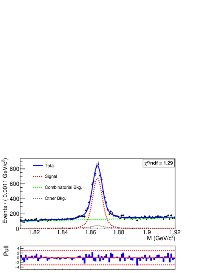
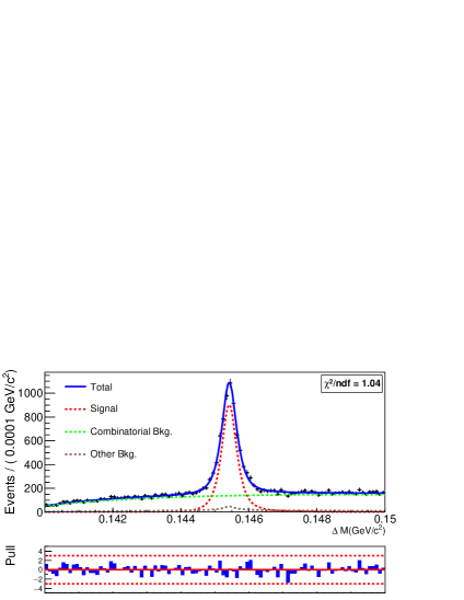
Figure 1: Projections of the fit for $D^{0}\!\rightarrow\!K^{0}_{S}\,K^{0}_{S}\,\pi^{+}\pi^{-}$ on $M$ (upper) and $\Delta M$ (lower). The brown dashed curve consists of slow pion, broken charm, and $D^{0}\!\rightarrow\!K^{0}_{S}\,K^{0}_{S}\,K^{0}_{S}$ backgrounds. The corresponding pull distributions [$=({\rm data}-{\rm fit\ result})/({\rm data\ uncertainty})$] are shown below each projection. The dashed red lines correspond to $\pm 3\sigma$ values.

We normalize the sensitivity of our search by counting the number of $D^{0}\!\rightarrow\!K^{0}_{S}\,\pi^{+}\pi^{-}$ decays observed in the same data set. The branching fraction for $D^{0}\!\rightarrow\!K^{0}_{S}\,K^{0}_{S}\,\pi^{+}\pi^{-}$ is calculated as

$$\mathcal{B}(D^{0}\!\rightarrow\!K^{0}_{S}\,K^{0}_{S}\,\pi^{+}\pi^{-}) =$$

$$\hskip-108.405pt\left(\frac{N_{K^{0}_{S}\,K^{0}_{S}\pi^{+}\pi^{-}}}{N_{K^{0}_{S}\pi^{+}\pi^{-}}}\right)\left(\frac{\varepsilon_{K^{0}_{S}\pi^{+}\pi^{-}}}{\varepsilon_{K^{0}_{S}\,K^{0}_{S}\pi^{+}\pi^{-}}}\right)\times\frac{\mathcal{B}(D^{0}\!\rightarrow\!K^{0}_{S}\,\pi^{+}\pi^{-})}{\mathcal{B}(K^{0}_{S}\!\rightarrow\!\pi^{+}\pi^{-})}\,,$$

where $N$ is the fitted yield for $D^{0}\!\rightarrow\!K^{0}_{S}\,K^{0}_{S}\,\pi^{+}\pi^{-}$ or $D^{0}\!\rightarrow\!K^{0}_{S}\,\pi^{+}\pi^{-}$ decays; $\varepsilon$ is the corresponding reconstruction efficiency, given that $K^{0}_{S}\!\rightarrow\!\pi^{+}\pi^{-}$; and $\mathcal{B}(K^{0}_{S}\!\rightarrow\!\pi^{+}\pi^{-})$ and $\mathcal{B}(D^{0}\!\rightarrow\!K^{0}_{S}\,\pi^{+}\pi^{-})$ are the world average branching fractions for $K^{0}_{S}\!\rightarrow\!\pi^{+}\pi^{-}$ and $D^{0}\!\rightarrow\!K^{0}_{S}\,\pi^{+}\pi^{-}$ [23]. The selection criteria for $D^{0}\!\rightarrow\!K^{0}_{S}\,\pi^{+}\pi^{-}$ are the same as those used for $D^{0}\!\rightarrow\!K^{0}_{S}\,K^{0}_{S}\,\pi^{+}\pi^{-}$, except that only one $K^{0}_{S}$ is required.

We determine $N_{K^{0}_{S}\pi^{+}\pi^{-}}$ from a two-dimensional binned fit (rather than unbinned, as the statistics are large) to the $M$ and $\Delta M$ distributions. The fitted ranges are $1.820~{}{\rm GeV}/c^{2}<M<1.910~{}{\rm GeV}/c^{2}$ and $0.143~{}{\rm GeV}/c^{2}<\Delta M<0.148~{}{\rm GeV}/c^{2}$ [30]. We use separate PDFs for correctly reconstructed signal, slow pion background, broken charm background, and combinatorial background. The small fraction of mis-reconstructed signal events are included in the PDF for combinatorial background. The functional forms of the PDFs are mostly the same as those used when fitting $D^{0}\!\rightarrow\!K^{0}_{S}\,K^{0}_{S}\,\pi^{+}\pi^{-}$ events. For the $\Delta M$ PDF for signal, the sum of a symmetric Gaussian and an asymmetric Student’s t function is used. In addition, the parameter $\sigma_{t}$ of the Student’s t function is taken to be a function of $M$, to account for correlations: $\sigma_{t}=\sigma_{0}+\sigma_{1}(M-m_{D^{0}})$, where $\sigma_{0}$ and $\sigma_{1}$ are floated parameters and $m_{D^{0}}$ is the $D^{0}$ mass [23]. For the $M$ PDF of broken charm background, the sum of a Gaussian and a second-order Chebychev polynomial is used. For the $M$ PDF of combinatorial background, a first-order Chebychev polynomial is used. There are a total of 10 floated parameters. The fit yields $1\,069\,870\pm 1831$ $D^{0}\!\rightarrow\!K^{0}_{S}\,\pi^{+}\pi^{-}$ decays. Projections of the fit are shown in Fig. 2. The fit quality is somewhat worse than that for the signal mode due to the very high statistics. We account for uncertainty in the signal shape when evaluating systematic uncertainties (below).

We evaluate the reconstruction efficiencies in Eq. (LABEL:eqn:br) using MC simulation. For $D^{0}\!\rightarrow\!K^{0}_{S}\,K^{0}_{S}\,\pi^{+}\pi^{-}$ decays, no decay model has been measured. Thus we generate this final state in several ways: via four-body phase space, via $D^{0}\!\rightarrow\!K^{*+}K^{*-}$ decays, via $D^{0}\!\rightarrow\!K_{S}^{0}\,K_{S}^{0}\,\rho^{0}$ decays, via $D^{0}\!\rightarrow\!f^{0}\rho^{0}$ decays, and via $D^{0}\!\rightarrow\!K^{*+}K_{S}^{0}\,\pi^{-}$ decays. The resulting reconstruction efficiencies are found to span a narrow range; the central value is taken as our nominal value, and the spread is taken as a systematic uncertainty. The $D^{0}\!\rightarrow\!K^{0}_{S}\,\pi^{+}\pi^{-}$ decays are generated according to a Dalitz model comprising $\rho^{0}\,\overline{K}^{\,0}$, $\omega\overline{K}^{\,0}$, $K^{*}(892)^{-}\pi^{+}$, $K^{*}_{0}(1430)^{-}\pi^{+}$, and $K^{*}_{2}(1430)^{-}\pi^{+}$ intermediate resonances. The resulting efficiencies are $\varepsilon_{K^{0}_{S}\,K^{0}_{S}\pi^{+}\pi^{-}}=(6.92\pm 0.02)\%$ and $\varepsilon_{K^{0}_{S}\pi^{+}\pi^{-}}=(14.97\pm 0.03)\%$, where the errors are statistical only. These values are subsequently corrected for small differences between data and MC simulation in particle identification (PID) and $K^{0}_{S}$ reconstruction efficiencies. The differences are measured using $D^{*+}\!\rightarrow\!D^{0}\pi^{+}_{s},\,D^{0}\!\rightarrow\!K^{-}\pi^{+}$ and $D^{*+}\!\rightarrow\!D^{0}\pi^{+}_{s},\,D^{0}\!\rightarrow\!K^{0}_{S}\pi^{0}$ decays, respectively. The overall correction factors are $0.930\pm 0.014$ for $D^{0}\!\rightarrow\!K^{0}_{S}\,K^{0}_{S}\,\pi^{+}\pi^{-}$ and $0.899\pm 0.007$ for $D^{0}\!\rightarrow\!K^{0}_{S}\,\pi^{+}\pi^{-}$. Inserting all values into Eq. (LABEL:eqn:br) along with the fitted yields and the PDG values [23] $\mathcal{B}(D^{0}\!\rightarrow\!K^{0}_{S}\,\pi^{+}\pi^{-})=(2.80\pm 0.18)\%$ and $\mathcal{B}(K^{0}_{S}\!\rightarrow\!\pi^{+}\pi^{-})=(69.20\pm 0.05)\%$ gives $\mathcal{B}(D^{0}\!\rightarrow\!K^{0}_{S}\,K^{0}_{S}\,\pi^{+}\pi^{-})=(4.82\pm 0.08)\times 10^{-4}$, where the quoted uncertainty is statistical only.

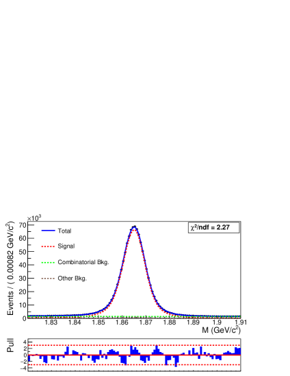
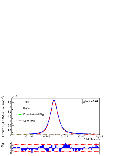
Figure 2: Projections of the fit for $D^{0}\!\rightarrow\!K^{0}_{S}\,\pi^{+}\pi^{-}$ on $M$ (upper) and $\Delta M$ (lower). The corresponding pull distributions [$=({\rm data}-{\rm fit\ result})/{\rm data\ uncertainty})$] are shown below each projection. The dashed red lines correspond to $\pm 3\sigma$ values.

The systematic uncertainties on the branching fraction are listed in Table 1. The uncertainty arising from the fixed parameters in signal and background PDFs is evaluated by varying these parameters and refitting. All 31 fixed parameters are sampled simultaneously from Gaussian distributions having mean values equal to the parameters’ nominal values and widths equal to their respective uncertainties. After sampling the parameters, the data are refit and the resulting signal yield recorded. The procedure is repeated 5000 times, and the root-mean-square (r.m.s.) of the 5000 signal yields is taken as the uncertainty due to the fixed parameters. When sampling the parameters, correlations among them are accounted for.

The uncertainty due to the fixed yield of broken charm background is evaluated by varying this yield (obtained from MC simulation) by $\pm 50$% and refitting. The fractional change in the signal yield is taken as the uncertainty. The uncertainty due to the fixed yield of $D^{0}\!\rightarrow\!K^{0}_{S}\,K^{0}_{S}\,K^{0}_{S}$ events is evaluated in a similar manner; in this case the $D^{0}\!\rightarrow\!K^{0}_{S}\,K^{0}_{S}\,K^{0}_{S}$ yield is varied by the fractional uncertainty in the branching fraction [23]. There is a small uncertainty due to the finite MC statistics used to evaluate the efficiencies $\varepsilon_{K^{0}_{S}\,K^{0}_{S}\pi^{+}\pi^{-}}$ and $\varepsilon_{K^{0}_{S}\pi^{+}\pi^{-}}$.

Uncertainty in track reconstruction gives rise to a possible difference in reconstruction efficiencies between data and MC simulation. This is evaluated in a separate study of $D^{*+}\!\rightarrow\!D^{0}\pi^{+}_{s},\,D^{0}\!\rightarrow\!K^{0}_{S}\,\pi^{+}\pi^{-}$ decays. The resulting uncertainty is 0.35% per track. As signal decays have two more charged tracks than normalization decays do, we take this uncertainty to be 0.70% on the branching fraction.

There is uncertainty due to $K^{0}_{S}$ reconstruction, which is found from a study of $D^{*+}\!\rightarrow\!D^{0}\pi^{+}_{s},\,D^{0}\!\rightarrow\!K^{0}_{S}\pi^{0}$ decays [22]. This uncertainty is 0.83% for $D^{0}\!\rightarrow\!K^{0}_{S}\,K^{0}_{S}\,\pi^{+}\pi^{-}$ and 0.36% for $D^{0}\!\rightarrow\!K^{0}_{S}\,\pi^{+}\pi^{-}$. These uncertainties are correlated between the two channels and partially cancel; however, as the respective $K^{0}_{S}$ daughters have different momentum spectra, for simplicity we take these uncertainties to be uncorrelated, which is conservative. The uncertainty due to PID criteria applied to the $\pi^{\pm}$ tracks is obtained from a study of $D^{*+}\!\rightarrow\!D^{0}\pi^{+}_{s},\,D^{0}\!\rightarrow\!K^{-}\pi^{+}$ decays. The resulting uncertainty is also momentum-dependent, and we take this uncertainty to also be uncorrelated between signal and normalization channels.

There is an uncertainty arising from the $|M(\pi^{+}\pi^{-})-m_{K^{0}_{S}}|>10$ MeV/$c^{2}$ requirement applied to reject $D^{0}\!\rightarrow\!K^{0}_{S}\,K^{0}_{S}\,K^{0}_{S}$ background. This is evaluated by varying this criterion from 8 MeV/$c^{2}$ to 15 MeV/$c^{2}$; the resulting fractional change in the signal yield is taken as the uncertainty. Finally, there is uncertainty in the PDG value $\mathcal{B}(K^{0}_{S}\!\rightarrow\!\pi^{+}\pi^{-})=0.6920\pm 0005$ (which enters $\varepsilon$), and the PDG value of the branching fraction for the normalization channel $D^{0}\!\rightarrow\!K^{0}_{S}\,\pi^{+}\pi^{-}$. The total systematic uncertainty is taken as the sum in quadrature of all individual uncertainties. The result is ${}^{+1.90}_{-2.07}\%$ for $D^{0}\!\rightarrow\!K^{0}_{S}\,K^{0}_{S}\,\pi^{+}\pi^{-}$, 0.71% for $D^{0}\!\rightarrow\!K^{0}_{S}\,\pi^{+}\pi^{-}$, and ${}^{+2.07}_{-2.23}\%$ for the ratio of branching fractions.

Table 1: Systematic uncertainties (fractional) for the branching fraction measurement.

Source	$K^{0}_{S}\,K^{0}_{S}\pi^{+}\pi^{-}$		$K^{0}_{S}\pi^{+}\pi^{-}$
	(%)		(%)
Fixed PDF parameters	0.14		0.09
$D^{0}\!\rightarrow\!K^{0}_{S}\,K^{0}_{S}\,K^{0}_{S}$ background	0.11		–
Broken charm background	0.98		–
MC statistics	0.26		0.17
PID efficiency correction	0.80		0.74
$K^{0}_{S}$ reconstruction efficiency	0.83		0.36
Tracking Efficiency	0.70
$M(\pi^{+}\pi^{-})$ veto efficiency	${}^{+0.42}_{-0.93}$		–
Fraction of mis-reconst. signal	${}^{+0.02}_{-0.03}$		–
$D^{0}\!\rightarrow\!K^{0}_{S}\,K^{0}_{S}\,\pi^{+}\pi^{-}$ decay model	0.73
$\mathcal{B}(K^{0}_{S}\!\rightarrow\!\pi^{+}\pi^{-})$	0.07		–
Total for $\mathcal{B}_{K^{0}_{S}\,K^{0}_{S}\pi^{+}\pi^{-}}/\mathcal{B}_{K^{0}_{S}\pi^{+}\pi^{-}}$	${}^{+2.07}_{-2.23}$

We measure the CP asymmetry $A_{CP}$ from the difference in signal yields for $D^{0}$ and $\overline{D}{}^{\,0}$ decays:

$$A^{\rm{det}}_{CP}{}=\frac{N(D^{0}\!\rightarrow\!f)-N(\overline{D}{}^{\,0}\!\rightarrow\!\overline{f})}{N(D^{0}\!\rightarrow\!f)+N(\overline{D}{}^{\,0}\!\rightarrow\!\overline{f})}\,.$$ (6)

The observable $A^{\rm{det}}_{CP}$ includes asymmetries in production and reconstruction:

$$A^{\rm{det}}_{CP} = A_{CP}+A_{\rm FB}+A_{\epsilon}^{\pi_{s}}\,,$$ (7)

where $A_{\rm FB}$ is the “forward-backward” production asymmetry [31] between $D^{*+}$ and $D^{*-}$ due to $\gamma^{*}-Z^{0}$ interference in $e^{+}e^{-}\!\rightarrow\!c\overline{c}$ ; and $A_{\epsilon}^{\pi_{s}}$ is the asymmetry in reconstruction efficiencies for $\pi^{\pm}_{s}$ tracks. We determine $A_{\epsilon}^{\pi_{s}}$ from a study of flavor-tagged $D^{*+}\!\rightarrow\!D^{0}\pi^{+}_{s},\,D^{0}\!\rightarrow\!K^{-}\pi^{+}$ decays and untagged $D^{0}\!\rightarrow\!K^{-}\pi^{+}$ decays [32]. In this study, $A_{\epsilon}^{\pi_{s}}$ is measured in bins of $p_{\rm T}$ and $\cos\theta_{\pi_{s}}$ of the $\pi^{\pm}_{s}$, where $p_{\rm T}$ is the transverse momentum and $\theta_{\pi_{s}}$ is the polar angle with respect to the $z$-axis, both evaluated in the laboratory frame. We subsequently correct for $A_{\epsilon}^{\pi_{s}}$ in $K^{0}_{S}\,K^{0}_{S}\,\pi^{+}\pi^{-}$ events by separately weighting $D^{0}$ and $\overline{D}{}^{\,0}$ decays:

$$w_{D^{0}} = 1-A_{\epsilon}^{\pi_{s}}(p_{\rm T},\,\cos\theta_{\pi_{s}})$$ (8)

$$w_{\overline{D}{}^{\,0}} = 1+A_{\epsilon}^{\pi_{s}}(p_{\rm T},\,\cos\theta_{\pi_{s}})\,.$$ (9)

After correcting for $A_{\epsilon}^{\pi_{s}}$, we obtain $A_{CP}^{\rm{cor}}=A_{CP}+A_{\rm FB}$. The asymmetry $A_{\rm FB}$ is an odd function of $\cos\theta^{*}$, and $A_{CP}$ is an even function, where $\theta^{*}$ is the polar angle between the $D^{*\pm}$ momentum and the $+z$ axis in the CM frame. We thus extract $A_{CP}$ and $A_{\rm FB}$ via

$$A_{CP} = \frac{A_{CP}^{\rm{cor}}(\cos\theta^{*})+A_{CP}^{\rm{cor}}(-\cos\theta^{*})}{2}$$ (10)

$$A_{\rm FB} = \frac{A_{CP}^{\rm{cor}}(\cos\theta^{*})-A_{CP}^{\rm{cor}}(-\cos\theta^{*})}{2}\,.$$ (11)

For this calculation, we define four bins of $\cos\theta^{*}$: $(-1.0,-0.4)$, $(-0.4,0)$, $(0,0.4)$ and $(0.4,1.0)$. We determine $A_{CP}^{\rm{cor}}$ for each bin by simultaneously fitting for $D^{0}$ and $\overline{D}{}^{\,0}$ signal yields for weighted events in that bin. We use the same PDF functions as used for the branching fraction measurement, and with the same fixed and floated parameters. The fixed shape parameters are taken to be the same for all $\cos\theta^{*}$ bins. The yields of combinatorial background for the $D^{0}$ and $\overline{D}{}^{\,0}$ samples are floated independently. The yields of broken charm and $D^{0}\!\rightarrow\!K^{0}_{S}\,K^{0}_{S}\,K^{0}_{S}$ backgrounds are fixed to MC values. The yield of slow pion background is also fixed: the total yield is fixed to the value obtained from the branching fraction fit, and the fraction assigned to $D^{0}$, $\overline{D}{}^{\,0}$, and each $\cos\theta^{*}$ bin is taken from MC simulation. The fitted parameters are $N(D^{0}\!\rightarrow\!f)$ and $A_{CP}^{\rm{cor}}$. The results for $A_{CP}^{\rm{cor}}$ are combined according to Eqs. (10) and (11) to obtain $A_{CP}$ and $A_{\rm FB}$. These values for the $\cos\theta^{*}$ bins are plotted in Fig. 3. Fitting the $A_{CP}$ values to a constant, we obtain $A_{CP}=(-2.51\pm 1.44)\%$.

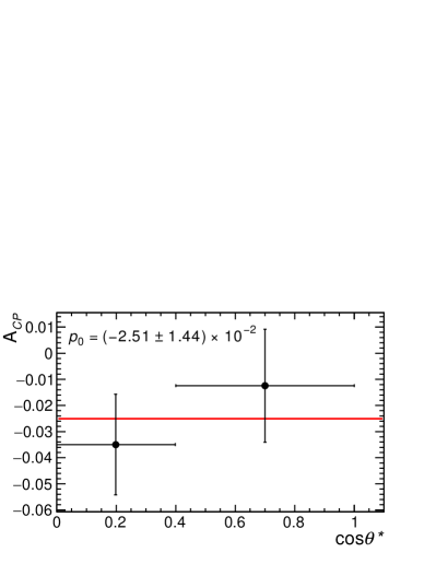
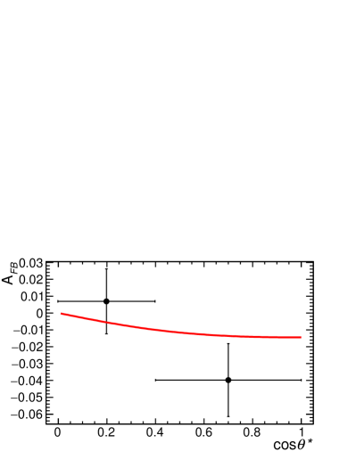
Figure 3: Values of $A_{CP}$ (upper) and $A_{\rm FB}$ (lower) in bins of $\cos\theta^{*}$. The red horizontal line in the $A_{CP}$ plot shows the result of fitting the points to a constant (“$p_{0}$”). The red curve in the $A_{\rm FB}$ plot shows the leading-order prediction for $A_{\rm FB}(e^{+}e^{-}\rightarrow c\overline{c})$ [33].

The systematic uncertainties for $A_{CP}$ are listed in Table 2. The uncertainty due to fixed parameters in the signal and background PDFs is evaluated in the same manner as done for the branching fraction: the various parameters are sampled from Gaussian distributions, and the fit is repeated. After 2000 trials, the r.m.s. of the distribution of $A_{CP}$ values is taken as the systematic uncertainty.

The uncertainty due to the fixed yields of backgrounds is evaluated in two ways. The uncertainties in the overall yields of broken charm and residual $D^{0}\!\rightarrow\!K^{0}_{S}\,K^{0}_{S}\,K^{0}_{S}$ backgrounds are evaluated in the same manner as done for the branching fraction measurement. In addition, the fixed fractions of the backgrounds between $D^{0}$ and $\overline{D}{}^{\,0}$ decays, and among the $\cos\theta^{*}$ bins, are varied by sampling these fractions from Gaussian distributions having widths equal to the respective uncertainties and repeating the fit. After 2000 trials, the r.m.s. of the resulting distribution of $A_{CP}$ values is again taken as the systematic uncertainty.

We assign a systematic uncertainty due to the choice of $\cos\theta^{*}$ binning by varying the number of bins from four to six, eight, and two. The differences between the lowest and highest values of $A_{CP}$ and the nominal result is assigned as the systematic uncertainty. There is also uncertainty arising from the $A_{\epsilon}^{\pi_{s}}$ values taken from Ref. [32]. We evaluate this by sampling $A_{\epsilon}^{\pi_{s}}$ values from Gaussian distributions and refitting for $A_{CP}$; after 2000 trials the r.m.s. of the fitted values is taken as the systematic uncertainty. The overall systematic uncertainty is the sum in quadrature of all individual uncertainties. The result is $(^{+0.35}_{-0.52})\%$, dominated by the uncertainty due to binning.

Table 2: Systematic uncertainties (absolute) for $A_{CP}$.

Sources		(%)
Fixed PDF parameters		$\pm 0.01$
$D^{0}\!\rightarrow\!K^{0}_{S}\,K^{0}_{S}\,K^{0}_{S}$ background		${}^{+0.02}_{-0.03}$
Broken charm background		${}^{+0.09}_{-0.07}$
Binning in $\cos\theta^{*}$		${}^{+0.33}_{-0.51}$
Reconstruction asymmetry $A_{\epsilon}^{\pi_{s}}$		$\pm 0.01$
Fixed background fractions		$\pm 0.04$
Total		${}^{+0.35}_{-0.52}$

To measure $a_{CP}^{T}$, we divide the data into four subsamples: $D^{0}$ decays with $C_{T}>0$ (${\rm yield}\!=\!N_{1}$) and $C_{T}<0$ (${\rm yield}\!=\!N_{2}$); and $\overline{D}{}^{\,0}$ decays with $-\overline{C}_{T}>0$ ($N_{3}$) and $-\overline{C}_{T}<0$ ($N_{4}$). Thus, $A_{T}=(N_{1}-N_{2})/(N_{1}+N_{2})$, $\bar{A}_{T}=(N_{3}-N_{4})/(N_{3}+N_{4})$, and $a_{CP}^{T}=(A_{T}-\bar{A}_{T})/2$. We fit the four subsamples simultaneously and take the fitted parameters to be $N_{1}$, $N_{3}$, $A_{T}$, and $a_{CP}^{T}$.

For this fit, we use the same PDF functions as used for the branching fraction measurement, and with the same fixed and floated parameters. The fixed shape parameters are taken to be the same for all four subsamples, as indicated by MC studies. The yield of combinatorial background is floated independently for all subsamples. The yield of slow pion background is fixed in the same way as done for the $A_{CP}$ fit. The fit gives $A_{T}=(-0.66\pm 2.01)\%$ and $a_{CP}^{T}=(-1.95\pm 1.42)\%$, where the uncertainties are statistical only. These values imply $\bar{A}_{T}=(+3.25\pm 1.98)\%$. Projections of the fit are shown in Fig. 4.

The systematic uncertainties for $a_{CP}^{T}$ are listed in Table 3. Several uncertainties that enter the branching fraction measurement cancel out for $a_{CP}^{T}$. The uncertainty arising from the fixed parameters in the signal and background PDFs is evaluated in the same manner as done for the branching fraction: the various parameters are sampled from Gaussian distributions, and the fit is repeated. After 5000 trials, the r.m.s. in the fitted values of $a_{CP}^{T}$ is taken as the systematic uncertainty. The uncertainties due to the fixed yields of broken charm and $D^{0}\!\rightarrow\!K^{0}_{S}\,K^{0}_{S}\,K^{0}_{S}$ backgrounds are also evaluated in the same manner as done for the branching fraction. Finally, we assign an uncertainty due to a possible difference in reconstruction efficiencies between decays with $C_{T},\,-\overline{C}_{T}>0$ and those with $C_{T},\,-\overline{C}_{T}<0$. These uncertainties are evaluated using MC simulation by taking the difference between generated and reconstructed values of $a_{CP}^{T}$. The total systematic uncertainty is taken as the sum in quadrature of all individual uncertainties; the result is $(^{+0.14}_{-0.12})\%$, dominated by the uncertainty due to efficiency variation.

Table 3: Systematic uncertainties (absolute) for the $a_{CP}^{T}$ measurement.

Source		(%)
Fixed PDF parameters		0.010
$D^{0}\!\rightarrow\!K^{0}_{S}\,K^{0}_{S}\,K^{0}_{S}$ background		${}^{+0.000}_{-0.013}$
Broken charm background		${}^{+0.014}_{-0.040}$
Efficiency variation with $C_{T},\,\overline{C}_{T}$		${}^{+0.14}_{-0.11}$
Total		${}^{+0.14}_{-0.12}$

In summary, using Belle data corresponding to an integrated luminosity of 922 fb^-1, we measure the branching fraction, $A_{CP}$, and $a_{CP}^{T}$ for $D^{0}\!\rightarrow\!K^{0}_{S}\,K^{0}_{S}\,\pi^{+}\pi^{-}$ decays. The branching fraction, measured relative to that for $D^{0}\!\rightarrow\!K^{0}_{S}\,\pi^{+}\pi^{-}$, is:

$$\frac{\mathcal{B}(D^{0}\!\rightarrow\!K^{0}_{S}\,K^{0}_{S}\,\pi^{+}\pi^{-})}{\mathcal{B}(D^{0}\!\rightarrow\!K^{0}_{S}\,\pi^{+}\pi^{-})} =$$

$$\hskip-50.58878pt[1.72\pm 0.03\,({\rm stat})\pm 0.04\,({\rm syst})\,]\times 10^{-2}\,.$$

Inserting the world average value $\mathcal{B}(D^{0}\!\rightarrow\!K^{0}_{S}\,\pi^{+}\pi^{-})=(2.80\pm 0.18)\%$ [23] gives

$$\mathcal{B}(D^{0}\!\rightarrow\!K^{0}_{S}\,K^{0}_{S}\,\pi^{+}\pi^{-}) =$$

$$\hskip-101.17755pt[4.82\pm 0.08\,({\rm stat})\pm^{+0.10}_{-0.11}\,({\rm syst})\pm 0.31\,({\rm norm})]\times 10^{-4}\,,$$

where the last uncertainty is due to $\mathcal{B}(D^{0}\!\rightarrow\!K^{0}_{S}\,\pi^{+}\pi^{-})$. The time-integrated CP asymmetry is measured to be

$$A_{CP}(D^{0}\!\rightarrow\!K^{0}_{S}\,K^{0}_{S}\,\pi^{+}\pi^{-}) =$$ (14)

$$\hskip-79.49744pt[-2.51\pm 1.44\,({\rm stat})\,^{+0.35}_{-0.52}\,({\rm syst})]\%\,.$$

The CP-violating asymmetry $a_{CP}^{T}$ is measured to be

$$a_{CP}^{T}(D^{0}\!\rightarrow\!K^{0}_{S}\,K^{0}_{S}\,\pi^{+}\pi^{-}) =$$ (15)

$$\hskip-65.04256pt[-1.95\,\pm 1.42\,({\rm stat})\,^{+0.14}_{-0.12}\,({\rm syst})]\%\,.$$

The branching fraction measurement is the most precise to date. The measurements of $A_{CP}$ and $a_{CP}^{T}$ are the first such measurements. We find no evidence of CP violation.

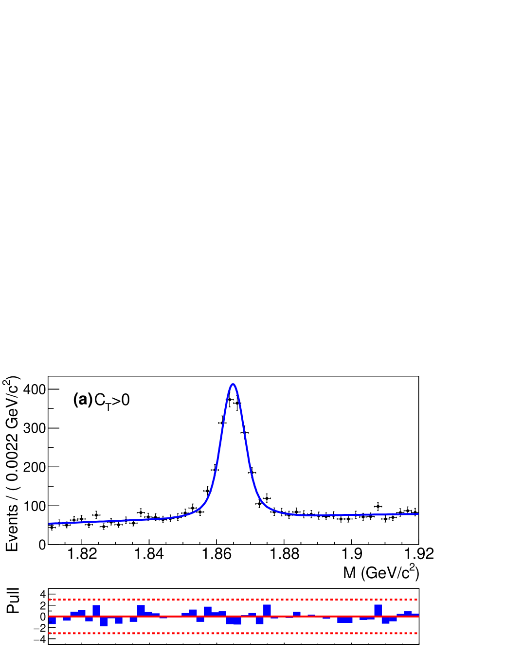
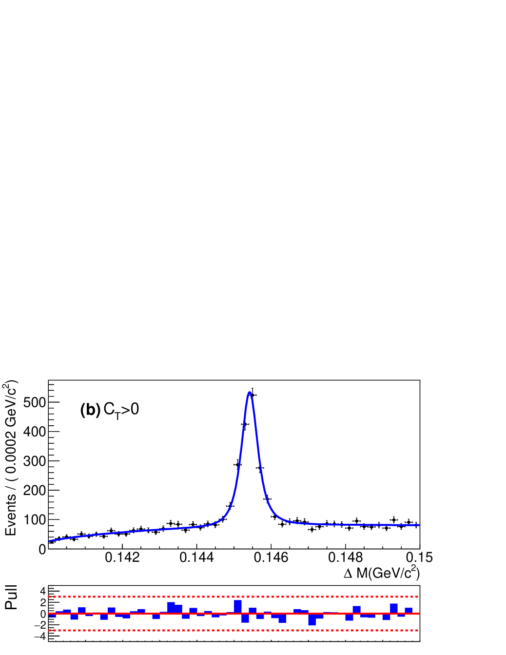
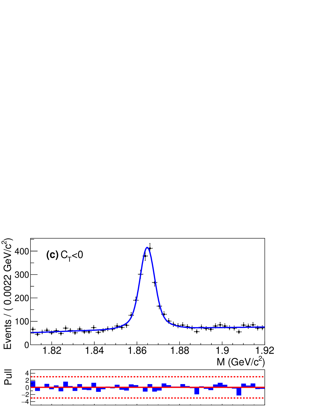
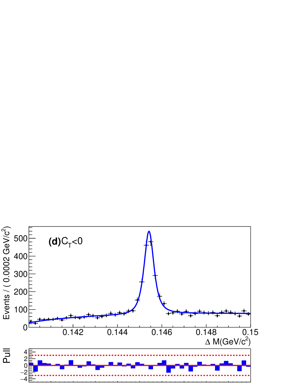
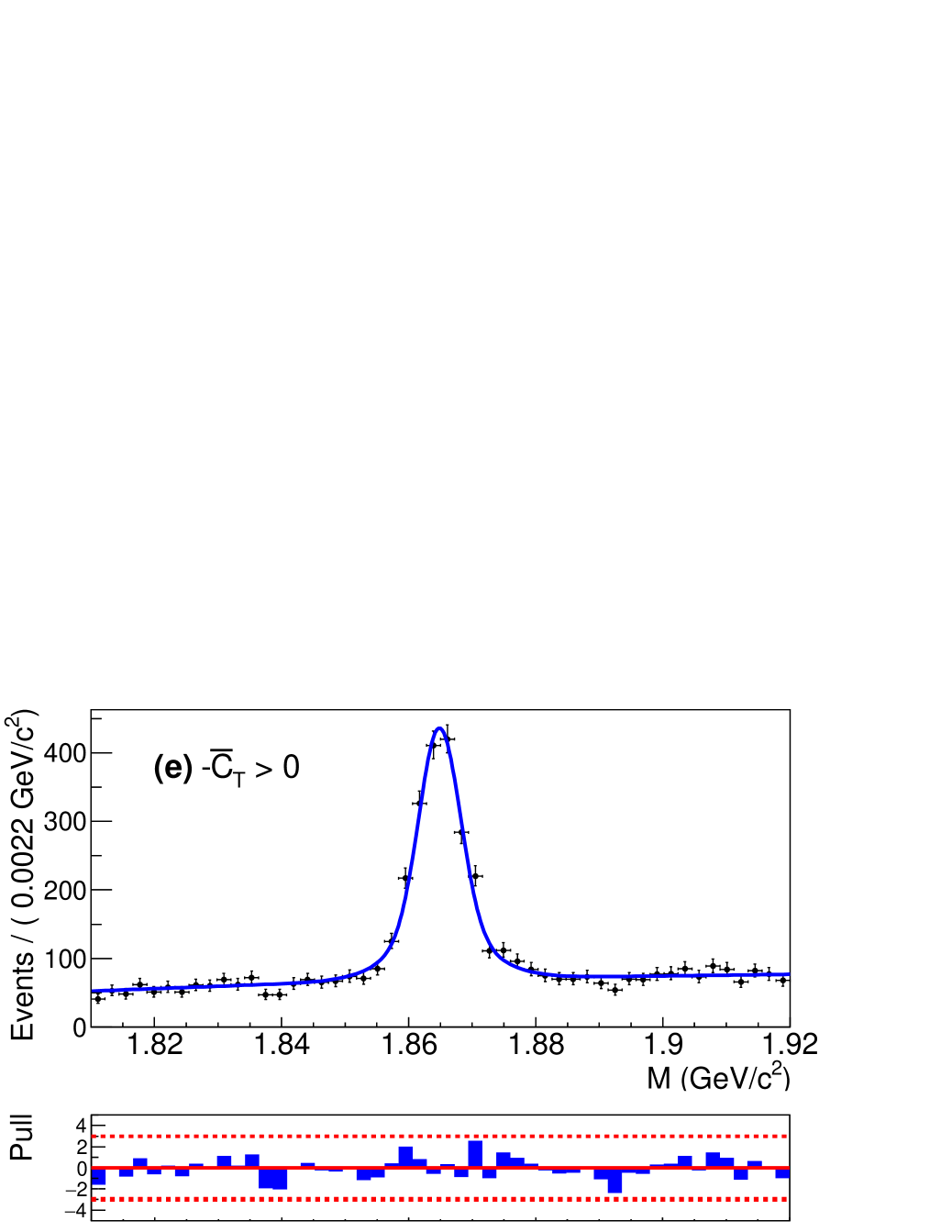
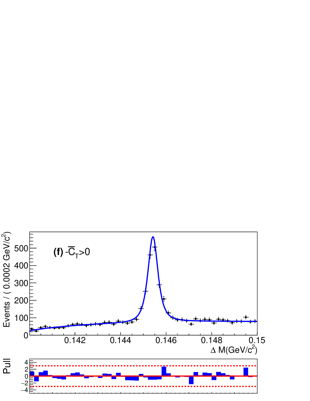
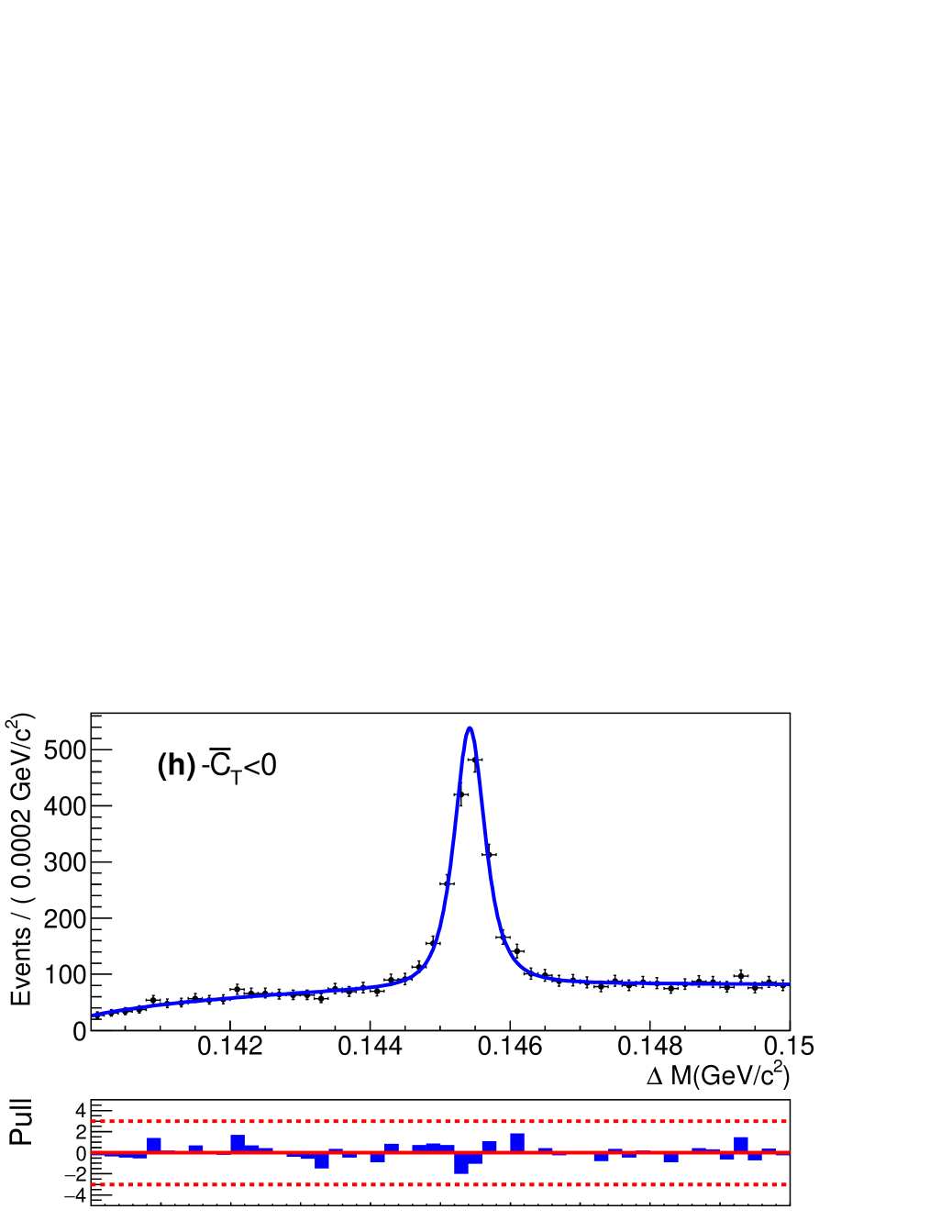
Figure 4: Projections of the fit for $a_{CP}^{T}$ in $M$ and $\Delta M$. (a) (b) the $D^{0}$ $C_{T}>0$ subsample; (c) (d) the $D^{0}$ $C_{T}<0$ subsample; (e) (f) the $\overline{D}{}^{\,0}$ $-\overline{C}_{T}>0$ subsample; and (g) (h) the $\overline{D}{}^{\,0}$ $-\overline{C}_{T}<0$ subsample.

We thank the KEKB group for the excellent operation of the accelerator, and the KEK cryogenics group for the efficient operation of the solenoid.

References

Canetti et al. [2012]
L. Canetti,
M. Drewes, and
M. Shaposhnikov,
New J. Phys. 14,
095012 (2012).
Farrar and Shaposhnikov [1994]
G. R. Farrar and
M. E. Shaposhnikov,
Phys. Rev. D 50,
774 (1994).
Allahverdi et al. [2021]
R. Allahverdi
et al., Open Jour. Astrophys.
4 (2021).
Sakharov [1967]
A. D. Sakharov,
Pisma Zh. Eksp. Teor. Fiz. 5,
32 (1967).
Kobayashi and Maskawa [1973]
M. Kobayashi and
T. Maskawa,
Prog. Theor. Phys. 49,
652 (1973).
Huet and Sather [1995]
P. Huet and
E. Sather,
Phys. Rev. D 51,
379 (1995).
[7]
Charge-conjugate modes are implicitly included unless noted
otherwise.
Albrecht et al. [1994]
H. Albrecht et al.
(ARGUS Collaboration), Zeit. Phys.
C 64, 375
(1994).
Link et al. [2005]
J. M. Link et al.
(FOCUS Collaboration), Phys. Lett.
B 607, 59
(2005).
Ablikim et al. [2020]
M. Ablikim et al.
(BESIII Collaboration), Phys. Rev.
D 102, 052006
(2020).
Grossman et al. [2007]
Y. Grossman,
A. L. Kagan, and
Y. Nir,
Phys. Rev. D 75,
036008 (2007).
Aaij et al. [2019]
R. Aaij et al.
(LHCb Collaboration), Phys. Rev.
Lett. 122, 211803
(2019).
Durieux and Grossman [2015]
G. Durieux and
Y. Grossman,
Phys. Rev. D 92,
076013 (2015).
Valencia [1989]
G. Valencia,
Phys. Rev. D 39,
3339 (1989).
Bensalem and London [2001]
W. Bensalem and
D. London,
Phys. Rev. D 64,
116003 (2001).
Kurokawa and Kikutani [2003]
S. Kurokawa and
E. Kikutani,
Nucl. Instrum. Meth. A 499,
1 (2003), and other papers in
this volume. T. Abe et al., Prog. Theor. Exp. Phys. 2013, 03A001
(2013) and references therein.
Abashian et al. [2002]
A. Abashian et al.
(Belle Collaboration), Nucl.
Instrum. Meth. A 479, 117
(2002), also see Section 2 in J. Brodzicka
et al., Prog. Theor. Exp. Phys. 2012, 04D001 (2012).
Natkaniec et al. [2006]
Z. Natkaniec
et al., Nucl. Instrum. Meth. A
560, 1 (2006).
Lange [2001]
D. J. Lange,
Nucl. Instrum. Meth. A 462,
152 (2001).
Brun et al. [1987]
R. Brun et al.,
GEANT 3.21, CERN Report DD/EE/84-1,
(1987).
Barberio and Was [1994]
E. Barberio and
Z. Was,
Comput. Phys. Commun. 79,
291 (1994).
Dash et al. [2017]
N. Dash et al.
(Belle Collaboration), Phys. Rev.
Lett. 119, 171801
(2017).
Zyla et al. [2020]
P. Zyla et al.
(Particle Data Group), PTEP
2020, 083C01
(2020).
Aubert et al. [2009]
B. Aubert et al.
(BaBar Collaboration), Phys. Rev.
D 79, 032002
(2009).
Lees et al. [2012]
J. P. Lees et al.
(BaBar Collaboration), Phys. Rev.
D 86, 112006
(2012).
Kronenbitter et al. [2012]
B. Kronenbitter
et al. (Belle Collaboration),
Phys. Rev. D 86,
071103 (2012).
Rohrken et al. [2012]
M. Rohrken et al.
(Belle Collaboration), Phys. Rev.
D 85, 091106
(2012).
Aaij et al. [2020]
R. Aaij et al.
(LHCb Collaboration), JHEP
03, 147 (2020).
James [2006]
F. E. James,
Statistical Methods in Experimental Physics; 2nd
ed. (World Scientific, Singapore,
2006).
[30] The fitted ranges are larger for the signal
mode in order to more accurately model the background level.
Berends et al. [1973]
F. Berends,
K. Gaemers, and
R. Gastmans,
Nucl. Phys. B63,
381 (1973).
Ko et al. [2011]
B. R. Ko et al.
(Belle Collaboration), Phys. Rev.
Lett. 106, 211801
(2011).
[33]
The leading-order prediction at GeV is ; see, for example, O. Nachtmann, Elementary Particle
Physics, Springer-Verlag (1989).