Global existence and singularity formation for the generalized Constantin-Lax-Majda equation with dissipation: The real line vs. periodic domains

Abstract

The question of global existence versus finite-time singularity formation is considered for the generalized Constantin-Lax-Majda equation with dissipation $-\Lambda^{\sigma}$, where $\widehat{{\Lambda}^{\sigma}}=|k|^{\sigma}$, both for the problem on the circle $x\in[-\pi,\pi]$ and the real line. In the periodic geometry, two complementary approaches are used to prove global-in-time existence of solutions for $\sigma\geq 1$ and all real values of an advection parameter $a$ when the data is small. We also derive new analytical solutions in both geometries when $a=0$, and on the real line when $a=1/2$, for various values of $\sigma$. These solutions exhibit self-similar finite-time singularity formation, and the similarity exponents and conditions for singularity formation are fully characterized. We revisit an analytical solution on the real line due to Schochet for $a=0$ and $\sigma=2$, and reinterpret it terms of self-similar finite-time collapse. The analytical solutions on the real line allow finite-time singularity formation for arbitrarily small data, even for values of $\sigma$ that are greater than or equal to one, thereby illustrating a critical difference between the problems on the real line and the circle. The analysis is complemented by accurate numerical simulations, which are able to track the formation and motion of singularities in the complex plane. The computations validate and extend the analytical theory.

1 Introduction

In this paper we investigate global well-posedness and singularity formation for the generalized Constantin-Lax-Majda (gCLM) model with dissipation,

$$\tilde{\omega}_{t}=-au\tilde{\omega}_{x}+\tilde{\omega}{\cal{H}}(\tilde{\omega})-\nu{\Lambda}^{\sigma}(\tilde{\omega}),\qquad\tilde{\omega}\in\mathbb{R},x\in\mathbb{S}\mbox{~{}or~{}}\mathbb{R},t>0,$$ (1)

$$u_{x}=\cal{H}\tilde{\omega},$$

$$\tilde{\omega}(x,t)\rightarrow 0\mbox{~{}for~{}}x\rightarrow\pm\infty\mbox{~{}when~{}}x\in\mathbb{R},$$

$$\tilde{\omega}(x,0)=\tilde{\omega}_{0}(x).$$

The equation is considered on both the circle $\mathbb{S}$ for $x\in[-\pi,\pi]$ and the real line $\mathbb{R}$. Here $\cal{H}$ is the usual Hilbert transform, which in the periodic case takes the form

$${\cal H}f(x)=\frac{1}{2\pi}PV\int_{-\pi}^{\pi}f(x^{\prime})\cot\left(\frac{x-x^{\prime}}{2}\right)\ dx^{\prime},$$

while for the problem on the real line

$${\cal H}f(x)=\frac{1}{\pi}PV\int_{-\infty}^{\infty}\frac{f(x^{\prime})}{x-x^{\prime}}\ dx^{\prime}.$$

The operator $\Lambda$ is given by ${\cal H}\partial_{x}$. The Hilbert transform has Fourier symbol

$$\hat{\cal{H}}=-i\mathrm{sgn}(k),$$

so that the symbols of $\Lambda$ and $\Lambda^{\sigma}$ are

$$\hat{\Lambda}(k)=|k|,\qquad\widehat{\Lambda^{\sigma}}(k)=|k|^{\sigma}.$$

Note that $-\Lambda^{2}$ gives the usual diffusion operator $\partial_{xx}$, and $-\Lambda^{\sigma}$ represents a generalized dissipation. The equation $u_{x}={\cal H}(\tilde{\omega})$ defines $u$ up to its mean, and we take the mean of $u$ to equal zero. The parameters $a$, $\sigma$ and $\nu$ satisfy $a\in\mathbb{R}$, $\sigma>0$ and $\nu>0$.

Constantin et al. [11] first introduced (LABEL:CLM) with $a=\nu=0$ as a simple 1D model to study finite-time singularity formation in the 3D incompressible Euler equations. It was later generalized by DeGregorio to include an advection term $u\tilde{\omega}_{x}$. Okamoto et al. [34] introduced the generalized advection term $au\tilde{\omega}_{x}$, with real parameter $a$, to investigate different relative weights of advection and vortex stretching, $\tilde{\omega}{\cal{H}}(\tilde{\omega})$. This generalized advection is motivated by recent studies of potential singularity formation in Euler and Navier-Stokes systems, which show that advection can have an unexpected smoothing effect [20, 21, 22, 26, 33]. We will refer to the Okamoto et al. model as the generalized Constantin-Lax-Majda (gCLM) equation. A diffusion term (can be also called by a viscosity term) $-\Lambda^{2}\tilde{\omega}=\partial_{x}^{2}\tilde{\omega}$ was first introduced into the Constantin et al. model (with $a=0$) by Schochet [36]. When $a=-1$ the gCLM equation with generalized dissipation is equivalent to the Cordoba-Cordoba-Fontelos equation [13], which has been extensively studied. For $\sigma>2$ one can interpret the term $-\nu{\Lambda}^{\sigma}(\tilde{\omega})$ in (LABEL:CLM) as a hyperviscosity which is widely used in many applications, see e.g. Ref. [38] for the hypervicosity in high temperature plasmas.

The dissipative gCLM system (LABEL:CLM) with $\sigma=2$ can be considered as a 1D model of the incompressible Navier-Stokes equations, which are written in terms of the vorticity $\boldsymbol{\omega}=\nabla\times\boldsymbol{u}$ as

$$\partial_{t}\boldsymbol{\omega} +\mathbf{u}\cdot\nabla\boldsymbol{\omega}=\boldsymbol{\omega}\cdot\nabla\mathbf{u}+\nu\nabla^{2}\boldsymbol{\omega},~{}~{}~{}\mathbf{x}\in\mathbb{R}^{3}\mbox{~{}or~{}}\mathbb{S}^{3},~{}t>0,$$ (2)

$$\mathbf{u} =\nabla\times(-\Delta)^{-1}\boldsymbol{\omega}.$$ (3)

The second equation above is the Biot-Savart law, which in free-space has an equivalent representation as a convolution integral

$$\mathbf{u}(\mathbf{x},t)=\frac{1}{4\pi}\int_{\mathbb{R}^{3}}\frac{(\mathbf{x}-\mathbf{y})\times\boldsymbol{\omega}(\mathbf{y},t)}{|\mathbf{x}-\mathbf{y}|^{3}}\ d\mathbf{y}.$$ (4)

The term $\boldsymbol{\omega}\cdot\nabla\mathbf{u}$ on the right-hand side of (2) is known as the vortex stretching term, and $\nabla\mathbf{u}$ can be represented via (4) as a matrix of singular integrals, which we denote by $S(\boldsymbol{\omega})$. The dissipative gCLM equation with $\sigma=2$ is obtained from (2)-(4) by replacing the advection term $\mathbf{u}\cdot\nabla\boldsymbol{\omega}$ with $au{\tilde{\omega}}_{x}$, the vortex stretching term $S(\boldsymbol{\omega})\boldsymbol{\omega}$ by its 1D analogue ${\cal H}({\tilde{\omega}}){\tilde{\omega}}$, and the diffusion term by ${\tilde{\omega}}_{xx}$. The Hilbert transform is the unique linear singular integral operator in 1D that, like $S(\boldsymbol{\omega})$, commutes with translations and dilations [11]. This motivates the replacement of $S(\boldsymbol{\omega})$ from the 3D equations with ${\cal H}({\tilde{\omega}})$ in the 1D model.

Singularities to (LABEL:CLM), when they occur, are generally found to be locally self-similar with the form

$$\tilde{\omega}=\frac{1}{\tau^{\beta}}f\left(\xi\right),\ \xi=\frac{x-x_{0}}{\tau^{\alpha}},\ \tau=t_{c}-t,$$ (5)

in a space-time neighborhood of $(x_{0},t_{c})$, where $t_{c}>0$ is the singularity time, $x_{0}\in\mathbb{R}$ is its location, and $\alpha$, $\beta$ are real similarity parameters. There are a number of results on finite-time singularity formation in the inviscid problem for (LABEL:CLM) with $\nu=0$, which we now briefly describe; see [31] for a more complete review. In this case of $\nu=0$, one has that $\beta=1$ while $\alpha$ depends on $a$. Constantin, Lax and Majda [11] present a closed-form exact solution to the initial value problem for (LABEL:CLM) with $a=0$. Their solution develops a singularity of the local form (5) with $\alpha=\beta=1$ for a class of analytic initial data. Castro and Cordoba [7] prove finite-time blow-up for $a<0$ using a Lyapunov-type argument. For $\epsilon-$small values of $a>0$, Elgindi and Jeong [17] and Chen et al. [9] prove the existence of singularities of the form (5) with $\beta=1$ and $\alpha$ approaching $1$ in the limit $a\to 0^{+}$.

More recently, [31] and [8] independently find an exact self-similar solution to the inviscid problem as a superposition of double-pole singularities for $a=1/2$ with $\alpha=1/3$ and $\beta=1$ ([31] further show that, beyond the particular cases $a=0$ and $a=1/2$, no exact solutions as a superposition of pole singularities exist). Lushnikov et al. [31] also perform numerical simulations over a wide range of $a$ and find the existence of a critical value $a_{c}=0.6890\ldots$ for which the self-similar blow up of solutions changes character. More precisely, they find self-similar collapse with $\alpha>0$ when $a<a_{c}$ for both $x\in\mathbb{S}$ and $\mathbb{R}$, expanding self-similar blow up with $\alpha<0$ when $a_{c}<a\leq 1$ and $x\in\mathbb{R}$, and ‘neither expanding nor collapsing’ blow-up with $\alpha=0$ when $a_{c}<a\leq 0.95$ and $x\in\mathbb{S}$ (with the expectation that the latter behavior occurs for $a$ going all the way up to, but not including, $a=1$). Here the terminology “collapse” or “wave collapse” was first introduced in [43] in analogy with gravitational collapse and has been widely used ever since to mean that the solution shrinks in $x$ as $t\to t_{c}$ while its amplitude diverges in that limit; see [43, 10, 40, 4, 25, 16, 30] for a more general description. Existence of the expanding similarity solution for $x\in\mathbb{R}$ and the ‘neither expanding nor collapsing’ similarity solution for $x\in\mathbb{S}$ are proven in [8], [9], when $a$ is near $1^{-}$. Analytical [23] and numerical [31] evidence is consistent with global well-posedness when $a\geq 1$ in the periodic problem, and $a>1$ in the problem on the real line. However, at present there is no proof of this for general analytic or $C^{\infty}$ initial data.

Much less is known about solutions to (LABEL:CLM) when there is nonzero dissipation. Schochet [36] constructs an explicit solution on the real line for $a=0$ and $\sigma=2$, which blows up in finite time. When $a=-1$, so that (LABEL:CLM) is the Cordoba-Cordoba-Fontelos equation, finite time blow up can occur for $\sigma<1/2$ [24, 27, 39], although there is global well-posedness for sufficiently small data [14]. Global well-posedness of the CCF equation for $\sigma\geq 1$ is shown in [13, 14, 24]. When $a\leq-2$ is even and $\sigma=1$, global well-posedness for small data in the periodic setting is shown in [42]. More recently, Chen [8] shows that for the problem on the real line, there exists self-similar blow up when $a$ is close to $1/2$ and $\sigma=2$, and global well-posedness for $\sigma\in[|a|^{-1},2]$ with $a<-1$. We note that for $a>-1$, there is no known coercive conserved quantity for general initial data, which complicates attempts to prove global well-posedness.

The focus of this paper is to further investigate conditions under which (LABEL:CLM) is well-posed globally in time, for different values of the parameters $a$ and $\sigma$. We find a surprising dependence of the global well-posedness on the domain of $x$, i.e., whether it is $\mathbb{S}$ or $\mathbb{R}$. In particular, we prove that the initial value problem (LABEL:CLM) with $\sigma\geq 1$ has global-in-time solutions for all sufficiently small data and all $a\in\mathbb{R}$, when the problem is considered on the periodic domain $x\in\mathbb{S}$. These solutions are analytic for $t>0$.

We present examples in the form of exact analytical solutions and numerical simulations which show this result does not hold on the real line $x\in\mathbb{R}$. The analytical results include new ‘pole dynamics’ solutions to (LABEL:CLM) – there are numerous examples of exact pole dynamics solutions in both Hamiltonian and dissipative systems, see e.g., [5, 37, 28, 29]. Our exact solutions for the problem on the real line form finite-time singularities of the type (5) for arbitrarily small initial data in $L^{2}$ and usually also in $L^{\infty}$. They include: (1) a solution for $a=1/2$ and $\sigma=1$ expressed as the sum of a complex conjugate (c.c.) pair of second order poles in $\omega$, (2) solutions for $a=0$ and $\sigma=1$ expressed as the sum of one or two c.c. pairs of first order poles in $\omega$, and (3) a solution for $a=0$ and $\sigma=0$ expressed as the sum of a c.c. pair of first order poles in $\omega$. We also revisit and slightly correct a previous example due to Schochet for $a=0$ and $\sigma=2$, which forms singularities in finite-time from arbitrarily small data, and reinterpret it as self-similar blow up. Overall, the exact solutions display different similarity exponents $\alpha$ and $\beta$, depending on the location and ‘strength’ (i.e., power or exponent) of their poles in the complex plane, and whether they impinge on the real line with a nonzero or zero velocity.

Additionally, we find a new pole dynamics solution to the periodic problem for $a=0$ with ‘marginal’ dissipation $\sigma=0$. This solution consists of a c.c. pair of simple poles and can form a finite-time singularity of the form (5) for data which is arbitrarily small in $L^{2}$, but not necessarily small in $L^{\infty}$. This supplies a lower bound in $\sigma$ for which a global existence theory in $L^{2}$ can apply, when $\nu$ is nonzero.

The analysis is complemented by accurate numerical simulations which confirm and build upon the analytical results in the periodic and real line problems. As part of the numerics, the formation and motion of singularities is tracked in the complex plane. When a singularity reaches the real line (at time $t_{c}$) a finite-time singularity of the form (5) occurs. We make use of two methods to trace singularities in the complex plane. One is based on the asymptotic decay of Fourier amplitudes, which gives precise (quantitative) information on the singularity that is closest to the real line. The other method, known as the AAA algorithm [32], utilizes rational function approximation to obtain information on singularities beyond the one closest to the real line.

Our analysis of the periodic problem makes use of two complementary approaches. We first prove that when $\sigma\geq 1,$ the solution exists globally in time for small initial data in the periodic Wiener algebra, which describes the set of functions with Fourier coefficients in $l^{1}$. A consequence of the proof is that solutions are analytic at all positive times in a strip in the complex plane that contains the real line, with the width of the strip growing linearly in time. The proof employs the method of Duchon and Robert [15], who developed it to show the existence of global vortex sheet solutions for certain types of small data. Other applications of this method to show global existence are [1, 2].

We also prove global-in-time existence of mild solutions with small initial data in $L^{2}$, when $\sigma>1$. A particular challenge in the proof is to obtain an exponential decay estimate for the solution operator when $t\gg 1$. We are able to do this, but the result relies in an essential way on the periodicity of the geometry. The proof guarantees that the solution at any time $t>0$ exists in $H^{\gamma}$ for all $1/2<\gamma<\min[1,\sigma-1/2]$. We further expect that solutions become analytic for $t>0$, even starting from rough $L^{2}$ data. This can be shown using the approach of Grujic and Kukavica [19], which has been used in several related problems to show analyticity of solutions on a strip which grows initially like $t^{1/\sigma}$ (see e.g., [2]). We do not provide details, and instead refer the interested reader to the relevant work.

The rest of this paper is organized as follows. After some mathematical preliminaries in §2, a solution operator is written in §2.1 using the Duhamel representation. Section 3 proves global existence for small periodic initial data with $\sigma\geq 1$ as a fixed point of the Duhamel representation by using a Wiener algebra approach. Section 4 proves global existence for small periodic initial data in $L^{2}$ with $\sigma>1$ using a mild solution approach. Section 5 focuses on the derivation of exact solutions on the real line and their relation to the self-similar form (5). Section 6 derives an exact solution to the periodic problem for $a=0$ and $\sigma=0$ which can develop a finite-time singularity for arbitrarily small data in $L^{2}$. Section 7 presents numerical results, with the numerical method described in §7.1, numerical results for the periodic problem given in §7.2, and numerical results for the problem on the real line discussed in §7.3. Concluding remarks are given in §8. An appendix, §A, provides a proof of inequality (12) used in the Wiener space analysis, and Lemmas 4.1 and 4.3 used in the mild solution analysis.

2 Preliminaries

By rescaling each of $t$ and $\tilde{\omega},$ we can eliminate $\nu$ from the problem. We therefore set $\nu=1$ without loss of generality, unless otherwise noted.

Notice that for any periodic function $f,$ we have $\int_{\mathbb{S}}f{\cal H}(f)\ dx=0.$ Also, $u\tilde{\omega}_{x}=(u\tilde{\omega})_{x}-\tilde{\omega}\mathcal{H}\tilde{\omega}$ has zero mean. Thus the mean of $\tilde{\omega}$ is preserved under the evolution (LABEL:CLM) on the circle. In the periodic problem, we make the decomposition $\tilde{\omega}=\omega+{\omega}_{av},$ where ${\omega}_{av}$ is the mean of $\tilde{\omega}$ and $\omega$ has zero mean. Substituting this decomposition in (LABEL:CLM) yields

$$(\omega+{\omega}_{av})_{t}+au(\omega+{\omega}_{av})_{x}=(\omega+{\omega}_{av})\mathcal{H}(\omega+{\omega}_{av})-\Lambda^{\sigma}(\omega+{\omega}_{av})\mbox{~{}for~{}}x\in\mathbb{S},$$ (6)

with $u$ now being defined through $u_{x}=\mathcal{H}(\omega);$ this is the same as the previous formula since the periodic Hilbert transform of a constant function is equal to zero. Since $({\omega}_{av})_{t}=({\omega_{av}})_{x}=\mathcal{H}({\omega}_{av})=\Lambda^{\sigma}({\omega}_{av})=0,$ we can rewrite (6) as

$$\omega_{t}+au\omega_{x}=\omega\mathcal{H}(\omega)+{\omega}_{av}\mathcal{H}(\omega)-\Lambda^{\sigma}\omega\mbox{~{}for~{}}x\in\mathbb{S},$$ (7)

with initial data $\omega(x,0)=\omega_{0}(x)$, which are used instead of the first and last equation in (LABEL:CLM) for the periodic problem. We continue to use (LABEL:CLM) for the problem on the real line, but omit the tilde from $\omega$, with the understanding that when $x\in\mathbb{R}$ the function $\omega$ is allowed to have a nonzero mean.

Notice the Hilbert transform also has the representation

$$\mathcal{H}\omega=-i(\omega_{+}-\omega_{-}),$$ (8)

where $\omega=\omega_{+}+\omega_{-}$ with $\omega_{+}$ analytic in the upper complex half-plane $\mathbb{C}^{+}$, and $\omega_{-}$ is analytic in the lower complex half-plane $\mathbb{C}^{-}$. In the periodic problem, $f_{+}=\sum_{k>0}\widehat{f}_{k}e^{ikx}$ and $f_{-}=\sum_{k<0}\widehat{f}_{k}e^{ikx}$ are the projections onto the upper and lower analytic components of $f$, respectively.

2.1 Solution operator in the periodic case

The solution to (7) can be written using the Duhamel representation

$$\omega(\cdot,t)=e^{-t\mathcal{L}}\omega_{0}+\int_{0}^{t}e^{-(t-\tau)\mathcal{L}}\left(-au\omega_{x}+\omega u_{x}\right)(\cdot,\tau)\ d\tau,$$ (9)

in which the operator $e^{-t\mathcal{L}}$ is defined by

$$e^{-t\mathcal{L}}f=\mathcal{F}^{-1}\left(e^{-t|k|^{\sigma}-it{\omega_{av}}\mathrm{sgn}(k)}\widehat{f}(k)\right)$$ (10)

where $\mathcal{F}$ is the Fourier transform operator. It is helpful to rewrite (9) slightly; we do so by first rewriting (7) using

$$u\omega_{x}=(u\omega)_{x}-u_{x}\omega=(u\omega)_{x}-\omega\mathcal{H}(\omega),$$

leading to

$$\omega_{t}=(1+a)\omega\mathcal{H}(\omega)-a(u\omega)_{x}+{\omega_{av}}\mathcal{H}(\omega)-\Lambda^{\sigma}\omega.$$

We again rewrite this using Duhamel’s principle, finding

$$\omega=e^{-t\mathcal{L}}\omega_{0}+\int_{0}^{t}e^{-(t-\tau)\mathcal{L}}\left[(1+a)\omega\mathcal{H}(\omega)-a(u\omega)_{x}\right](\cdot,\tau)\ d\tau.$$ (11)

We use again the fact that for any periodic function $f,$ the integral $\int_{\mathbb{S}}f\mathcal{H}(f)\ dx=0;$ introducing the operator $\mathbb{P}_{0}$ to be the projection which zeroes out the mean of a periodic function, we have

$$\mathbb{P}_{0}\left[(1+a)\omega\mathcal{H}(\omega)-a(u\omega)_{x}\right]=\left[(1+a)\omega\mathcal{H}(\omega)-a(u\omega)_{x}\right].$$

We then use this with (11) as the basis for introducing an operator $\mathcal{T},$

$$\mathcal{T}(\omega)=e^{-t\mathcal{L}}\omega_{0}+\int_{0}^{t}e^{-(t-\tau)\mathcal{L}}\mathbb{P}_{0}\left[(1+a)\omega\mathcal{H}(\omega)-a(u\omega)_{x}\right](\cdot,\tau)\ d\tau.$$

We will obtain solutions of the gCLM equation with dissipation by finding a fixed point of $\mathcal{T}$. As we have said above, we will do this twice, once in function spaces based on the Wiener algebra, and once in $L^{2}$-based Sobolev spaces.

3 Small global solutions in spaces based on the Wiener algebra

In this section we will prove global existence of small solutions when the initial data is taken from the Wiener algebra. This uses an adaptation of the argument of Duchon and Robert used to prove existence of small global vortex sheets [15]. The unregularized vortex sheet is an elliptic problem in space-time, but the method has also been applied to parabolic problems in [1, 2].

3.1 Function spaces and operators

We denote the periodic Wiener algebra as $B_{0};$ this is the set of functions $f:\mathbb{S}\rightarrow\mathbb{R}$ such that the norm

$$\|f\|_{B_{0}}=\sum_{k\in\mathbb{Z}}|\hat{f}(k)|$$

is finite.

For $\varpi>0$ and $\theta\geq 0,$ we define the function space $\mathcal{B}_{\varpi}^{\theta}$ to be the set of periodic functions continuous in time with values in $B_{0},$ such that the norm

$$\|h\|_{\varpi,\theta}=\sum_{k\in\mathbb{Z}}(1+|k|^{\theta})\sup_{t\in[0,\infty)}e^{\varpi t|k|}|\hat{h}(k,t)|$$

is finite. We will demonstrate that this is a Banach algebra. First, note that for all $k\in\mathbb{Z},$ for all $j\in\mathbb{Z},$ we have

$$|k|^{\theta}\leq\max\{1,2^{\theta-1}\}\left(|k-j|^{\theta}+|j|^{\theta}\right).$$ (12)

(We prove this inequality in Appendix A.1.) We denote $C=\max\{1,2^{\theta-1}\}.$ We compute the norm of $fg,$ for $f\in\mathcal{B}_{\varpi}^{\theta}$ and $g\in\mathcal{B}_{\varpi}^{\theta}:$

$$\|fg\|_{\varpi,\theta}=\sum_{k\in\mathbb{Z}}(1+|k|^{\theta})\sup_{t\in[0,\infty)}e^{\varpi t|k|}|\widehat{(fg)}(k,t)|\\ \leq C\sum_{(k,j)\in\mathbb{Z}^{2}}\left(1+|k-j|^{\theta}+|j|^{\theta}\right)\left[\sup_{t\in[0,\infty)}e^{\varpi t|k-j|}|\hat{f}(k-j,t)|\right]\left[\sup_{t\in[0,\infty)}e^{\varpi t|j|}|\hat{g}(j,t)|\right].$$ (13)

We sum first in $k$ and then in $j,$ finding

$$\|fg\|_{\varpi,\theta}\leq C\|g\|_{\varpi,0}\|f\|_{\varpi,\theta}+C\|f\|_{\varpi,0}\|g\|_{\varpi,\theta}\leq 2C\|f\|_{\varpi,\theta}\|g\|_{\varpi,\theta}.$$

For any $\varpi>0$ and $\theta\geq 0,$ we let $\mathcal{B}_{\varpi,0}^{\theta}$ be the subspace of $\mathcal{B}_{\varpi}^{\theta}$ of functions with zero mean. We then define the integral operator $I^{+}:\mathcal{B}_{\varpi}^{\theta}\rightarrow\mathcal{B}_{\varpi,0}^{\theta+\sigma}$ by

$$(I^{+}h)(\cdot,t)=\int_{0}^{t}e^{-(t-\tau)\mathcal{L}}\mathbb{P}_{0}h(\cdot,\tau)\ d\tau.$$

We compute the operator norm of $I^{+}.$ The norm for $\mathcal{B}_{\varpi,0}^{\theta+\sigma}$ is the same as for $\mathcal{B}_{\varpi}^{\theta+\sigma},$ except that the $k=0$ mode is excluded from the summation. Therefore we have

$$\|I^{+}h\|_{\varpi,\theta+\sigma}=\sum_{k\in\mathbb{Z}\setminus\{0\}}(1+|k|^{\theta+\sigma})\sup_{t\in[0,\infty)}e^{\varpi t|k|}\left|\int_{0}^{t}e^{-|k|^{\sigma}(t-\tau)-i{\omega_{av}}\mathrm{sgn}(k)(t-\tau)}\hat{h}(\cdot,\tau)\ d\tau\right|.$$

We use the triangle inequality and rearrange the exponentials, finding

$$\|I^{+}h\|_{\varpi,\theta+\sigma}=\sum_{k\in\mathbb{Z}\setminus\{0\}}(1+|k|^{\theta+\sigma})\sup_{t\in[0,\infty)}e^{(\varpi|k|-|k|^{\sigma})t}\int_{0}^{t}e^{|k|^{\sigma}\tau}|\hat{h}(k,\tau)|\ d\tau.$$

We adjust factors of the weights, arriving at

$$\|I^{+}h\|_{\varpi,\theta+\sigma}=\sum_{k\in\mathbb{Z}\setminus\{0\}}\left(\frac{1+|k|^{\theta+\sigma}}{1+|k|^{\theta}}\right)\Bigg{(}\sup_{t\in[0,\infty)}e^{(\varpi|k|-|k|^{\sigma})t}\cdot\\ \cdot\int_{0}^{t}e^{(|k|^{\sigma}-\varpi|k|)\tau}\left[(1+|k|^{\theta})e^{\varpi|k|\tau}|\hat{h}(k,\tau)|\right]\ d\tau\Bigg{)}.$$ (14)

We estimate this by taking the supremum two more times, once with respect to $\tau$ and once with respect to $k,$ and then rearranging:

$$\|I^{+}h\|_{\varpi,\theta+\sigma}\leq\left(\sum_{k\in\mathbb{Z}\setminus\{0\}}(1+|k|^{\theta})\sup_{\tau\in[0,\infty)}e^{\varpi|k|\tau}|\hat{h}(k,\tau)|\right)\\ \left(\sup_{k\in\mathbb{Z}\setminus\{0\}}\left(\frac{1+|k|^{\theta+\sigma}}{1+|k|^{\theta}}\right)\sup_{t\in[0,\infty)}e^{(\varpi|k|-|k|^{\sigma})t}\int_{0}^{t}e^{(|k|^{\sigma}-\varpi|k|)\tau}\ d\tau\right).$$ (15)

We identify the first factor on the right-hand side as simply being $\|h\|_{\varpi,\theta},$ and we evaluate the last integral and simplify. These considerations yield the following:

$$\|I^{+}h\|_{\varpi,\theta+\sigma}\leq\|h\|_{\varpi,\theta}\left(\sup_{k\in\mathbb{Z}\setminus\{0\}}\left(\frac{1+|k|^{\theta+\sigma}}{1+|k|^{\theta}}\right)\sup_{t\in[0,\infty)}\frac{1-e^{(\varpi|k|-|k|^{\sigma})t}}{|k|^{\sigma}-\varpi|k|}\right).$$

The last denominator on the right-hand side is positive as long as $\sigma\geq 1$ and $\varpi<1.$ With these conditions, we may then ignore the negative term in the numerator, arriving at

$$\|I^{+}h\|_{\varpi,\theta+\sigma}\leq\|h\|_{\varpi,\theta}\left(\sup_{k\in\mathbb{Z}\setminus\{0\}}\frac{1+|k|^{\theta+\sigma}}{(1+|k|^{\theta})(|k|^{\sigma}-\varpi|k|)}\right).$$

We then estimate this using $1\leq|k|^{\sigma}$ and simplifying, arriving at

$$\|I^{+}h\|_{\varpi,\theta+\sigma}\leq\frac{\|h\|_{\varpi,\theta}}{1-\varpi}.$$ (16)

We need an entirely analagous bound for the composition operator $I^{+}\partial_{x}.$ The above proof of the estimate (16) works just the same to show that $I^{+}\partial_{x}$ maps $\mathcal{B}_{\varpi}^{\theta}$ to $\mathcal{B}_{\varpi}^{\theta+\sigma-1},$ with the estimate

$$\|I^{+}\partial_{x}h\|_{\varpi,\theta+\sigma-1}\leq\frac{\|h\|_{\varpi,\theta}}{1-\varpi}.$$ (17)

We also need to demonstrate the boundedness of the semigroup, acting on $B_{0}.$ Letting $h\in B_{0},$ we consider the norm of $e^{-t\mathcal{L}}h:$

$$\|e^{-t\mathcal{L}}h\|_{\varpi,0}=2\sum_{k\in\mathbb{Z}}\sup_{t\in[0,\infty)}e^{\varpi t|k|}e^{-|k|^{\sigma}t}|\hat{h}(k)|\leq 2\|h\|_{B_{0}}\sup_{k\in\mathbb{Z}}\sup_{t\in[0,\infty)}e^{(\varpi|k|-|k|^{\sigma})t}.$$

With $\sigma\geq 1$ and $\varpi<1,$ we may estimate this as

$$\|e^{-t\mathcal{L}}h\|_{\varpi,0}\leq 2\|h\|_{B_{0}}.$$

3.2 Existence of a solution

In the current notation, our operator $\mathcal{T}$ may be expressed as

$$\mathcal{T}\omega=e^{-t\mathcal{L}}\omega_{0}+\left(I^{+}\left[(1+a)\omega\mathcal{H}(\omega)-a(u\omega)_{x}\right]\right)(t).$$ (18)

A fixed point of (18) is a solution of the initial value problem for (7).

We see that if $\omega_{0}\in B_{0}$ and if $\varpi<1$ and $\sigma\geq 1,$ then $\mathcal{T}$ maps $\mathcal{B}_{\varpi}^{0}$ to itself. We want to show that there exists $X\subseteq\mathcal{B}_{\varpi}^{0}$ such that $\mathcal{T}$ is a contraction on $X.$ We let $X$ be the ball of radius $r_{0}$ centered at $e^{-t\mathcal{L}}\omega_{0},$ and we denote $r_{1}=\|\omega_{0}\|_{B_{0}}.$ We will show that $\mathcal{T}$ is a contraction on $X$ for an appropriate choice of $r_{0}$ and $r_{1}.$ Note that for any $\omega\in X,$ we have $\|\omega\|_{\varpi,0}\leq r_{0}+r_{1}.$

We have two properties to establish: that $\mathcal{T}:X\rightarrow X,$ and that there exists $\lambda\in(0,1)$ such that for any $\omega_{1}\in X$ and for any $\omega_{2}\in X,$

$$\|\mathcal{T}(\omega_{1}-\omega_{2})\|_{\varpi,0}\leq\lambda\|\omega_{1}-\omega_{2}\|_{\varpi,0}.$$ (19)

To show that $\mathcal{T}$ maps $X$ to $X,$ we let $\omega\in X$ be given, and we need to establish that

$$\left\|I^{+}\left[(1+a)\omega\mathcal{H}(\omega)-a(u\omega)_{x}\right]\right\|_{\varpi,0}\leq r_{0}.$$

We immediately have

$$\left\|I^{+}\left[(1+a)\omega\mathcal{H}(\omega)-a(u\omega)_{x}\right]\right\|_{\varpi,0}\leq\frac{|1+a|}{1-\varpi}(r_{0}+r_{1})^{2}+|a|\|I^{+}(u\omega)\|_{\varpi,1}.$$

We then bound this as

$$\left\|I^{+}\left[(1+a)\omega\mathcal{H}(\omega)-a(u\omega)_{x}\right]\right\|_{\varpi,0}\leq\frac{|1+a|}{1-\varpi}(r_{0}+r_{1})^{2}+\frac{|a|}{1-\varpi}(r_{0}+r_{1})\|u\|_{\varpi,0}.$$

We also have $\|u\|_{\varpi,0}\leq\|\omega\|_{\varpi,0},$ so that

$$\left\|I^{+}\left[(1+a)\omega\mathcal{H}(\omega)-a(u\omega)_{x}\right]\right\|_{\varpi,0}\leq\frac{|1+a|+|a|}{1-\varpi}(r_{0}+r_{1})^{2}.$$

Our first condition that $r_{0}$ and $r_{1}$ must satisfy, then, is

$$\frac{|1+a|+|a|}{1-\varpi}(r_{0}+r_{1})^{2}\leq r_{0}.$$ (20)

Next, we work on establishing (19). To begin, we express the difference $\mathcal{T}(\omega_{1}-\omega_{2}),$ doing some adding and subtracting:

$$\mathcal{T}(\omega_{1}-\omega_{2})=\int_{0}^{t}e^{-(t-\tau)\mathcal{L}}\left[(1+a)\omega_{1}\mathcal{H}(\omega_{1})-a(u_{1}\omega_{1})_{x}\right](\cdot,\tau)\ d\tau\\ -\int_{0}^{t}e^{-(t-\tau)\mathcal{L}}[(1+a)\omega_{2}\mathcal{H}(\omega_{2})-a(u_{2}\omega_{2})_{x}](\cdot,\tau)\ d\tau\\ =A_{1}+A_{2}+A_{3}+A_{4},$$ (21)

where the $A_{i}$ are given by

$$A_{1}=\int_{0}^{t}e^{-(t-\tau)\mathcal{L}}[(1+a)(\omega_{1}-\omega_{2})\mathcal{H}(\omega_{1})](\tau)\ d\tau,$$

$$A_{2}=\int_{0}^{t}e^{-(t-\tau)\mathcal{L}}[(1+a)\omega_{2}(\mathcal{H}(\omega_{1})-\mathcal{H}(\omega_{2})](\cdot,\tau)\ d\tau,$$

$$A_{3}=-\int_{0}^{t}e^{-(t-\tau)\mathcal{L}}a((u_{1}-u_{2})\omega_{1})_{x}(\cdot,\tau)\ d\tau,$$

$$A_{4}=-\int_{0}^{t}e^{-(t-\tau)\mathcal{L}}a(u_{2}(\omega_{1}-\omega_{2})_{x})(\cdot,\tau)\ d\tau.$$

We may estimate these as follows:

$$\|A_{1}\|_{\varpi,0}\leq\frac{|1+a|}{1-\varpi}(r_{0}+r_{1})\|\omega_{1}-\omega_{2}\|_{\varpi,0},$$

$$\|A_{2}\|_{\varpi,0}\leq\frac{|1+a|}{1-\varpi}(r_{0}+r_{1})\|\omega_{1}-\omega_{2}\|_{\varpi,0},$$

$$\|A_{3}\|_{\varpi,0}\leq\frac{|a|}{1-\varpi}(r_{0}+r_{1})\|\omega_{1}-\omega_{2}\|_{\varpi,0},$$

$$\|A_{4}\|_{\varpi,0}\leq\frac{|a|}{1-\varpi}(r_{0}+r_{1})\|\omega_{1}-\omega_{2}\|_{\varpi,0}.$$

We combine these estimates to find

$$\|\mathcal{T}(\omega_{1}-\omega_{2})\|_{\varpi,0}\leq\frac{2(|1+a|+|a|)}{1-\varpi}(r_{0}+r_{1})\|\omega_{1}-\omega_{2}\|_{\varpi,0}.$$

Thus, our second condition which $r_{0}$ and $r_{1}$ must satisfy is

$$\frac{2(|1+a|+|a|)}{1-\varpi}(r_{0}+r_{1})<1.$$ (22)

To demonstrate that (20) and (22) may be satisfied, we take $r_{1}=r_{0},$ and we will choose $r_{1}.$ In this case, (20) becomes

$$r_{1}\leq\frac{1-\varpi}{4(|1+a|+|a|)},$$ (23)

while (22) becomes

$$r_{1}<\frac{1-\varpi}{4(|1+a|+|a|)}.$$ (24)

Of course (24) implies (23).

We have proved the following theorem:

Theorem 3.1

Let $a\in\mathbb{R},$ ${\omega_{av}}\in\mathbb{R},$ and $\sigma\geq 1$ be given. Let $\omega_{0}\in B_{0}$ be given, such that $\omega_{0}$ has zero mean and such that $\|\omega_{0}\|_{B_{0}}<\frac{1}{4(|1+a|+|a|)}.$ Let $\varpi\in(0,1)$ be given such that $\|\omega_{0}\|_{B_{0}}<\frac{1-\varpi}{4(|1+a|+|a|)}.$ Then the initial value problem for (7) with initial data $\omega_{0}$ has a unique solution $\omega\in\mathcal{B}_{\varpi}^{0}.$

We make a few remarks on Theorem 3.1. Since the solution is in $\mathcal{B}_{\varpi}^{0}$ with $\varpi>0,$ we know automatically that the solution exists for all $t\in[0,\infty),$ and that the solution is analytic at all positive times with radius of analyticity at least $\varpi t.$ Next, we notice that the value of $a$ does not matter as far as whether we can get global existence of a solution, except that it does affect the maximum allowable size of the data; specifically, for larger $|a|,$ we need to take the data smaller. As noted above, $\varpi$ is the rate at which analyticity is gained; if we want this to be larger, the data must be taken smaller. Finally we note that the value of $\omega_{av}$ does not affect the allowable size of the data or the rate at which analyticity is gained.

4 Mild solutions with data in $L^{2}$

In this section we complement Theorem 3.1 with another theorem on existence of small global solutions, now taking initial data in $L^{2}.$ In this approach, we will need more detailed mapping properties for the semigroup associated to the diffusive term than in the Wiener algebra case; we establish these properties in Section 4.2 below.

4.1 Function spaces and preliminary Lemmas

Throughout we use the notation $L^{2},H^{s}$ etc. to denote the spaces $L^{2}[-\pi,\pi]$, $H^{s}[-\pi,\pi]$ (with periodic boundary conditions) and so forth. We consider data and solutions with finite $L^{2}$ norm, i.e., finite energy. Hence, it will be convenient to work with the norm in homogeneous Sobolev spaces $\dot{H}^{s}$, defined by

$$\|f\|^{2}_{\dot{H}^{s}}=\sum_{k=-\infty}^{\infty}|k|^{2s}|\widehat{f}(k)|^{2},~{}~{}~{}s\in\mathbb{R}.$$

Note that if $f\in L^{2}$ then $f\in\dot{H}^{s}$ if and only if $f\in H^{s}$. We denote the subspace of functions in $L^{2}$ with zero mean as

$$\mathring{L}^{2}=\left\{f\in L^{2}\mid\int_{-\pi}^{\pi}f\ dx=0\right\}.$$

If a function $f$ has zero mean, then by Poincare’s inequality $\|f\|_{L^{2}}\leq c\|f_{x}\|_{L^{2}}$ so that $\dot{H}^{1}\subset\mathring{L}^{2}$. In particular, $\|\mathcal{H}\omega\|_{L^{2}}=\|\omega_{+}+\omega_{-}\|_{L^{2}}\leq c\|\omega_{x}\|_{L^{2}}$, but note that if a function $f$ has nonzero mean its $L^{2}$ norm cannot in general be bounded by the $L^{2}$ norm of its derivative.

In the fixed point analysis, we make use of the adapted space

$$X_{\infty}^{\eta}=\left\{\omega:\mathbb{S}\times[0,\infty)\rightarrow\mathbb{R}\mid\omega\in L^{\infty}([0,\infty);L^{2}),\sup_{0<t<\infty}t^{\eta/\sigma}\|\omega\|_{\dot{H}^{\eta}}<\infty\right\},$$

where $\sigma>0$ and $\eta>0$, with norm

$$\|\omega\|_{X_{\infty}^{\eta}}=\mbox{max}\left(\sup_{0<t<\infty}\|\omega\|_{L^{2}},\sup_{0<t<\infty}t^{\eta/\sigma}\|\omega\|_{\dot{H}^{\eta}}\right).$$

The factor of $t^{\eta/\sigma}$ is motivated by the estimate in Lemma 4.2 below with $s=\eta$ and $r=0$.

We will make use of the following elementary result, which is proven in the appendix:

Lemma 4.1

Let $\hat{q}>0$, $0\leq\hat{\alpha}<1$, and let ${\hat{\beta}}$ and ${\hat{\delta}}$ be nonnegative numbers with $0\leq\hat{\alpha}+{\hat{\beta}}\leq 1$ and $0\leq{\hat{\beta}}+{\hat{\delta}}<1$. Then there exists a positive constant $C$ such that

$$\int_{0}^{t}\frac{e^{-{\hat{q}}(t-\tau)}}{(t-\tau)^{\hat{\alpha}}}\frac{t^{\hat{\delta}}}{\tau^{{\hat{\beta}}+{\hat{\delta}}}}\ d\tau<C,$$ (25)

where $C$ is independent of $t\in[0,\infty).$

4.2 Operator estimates

We estimate the smoothing properties of the semigroup $e^{-t\mathcal{L}}$ for $t>0$. First, it is clear that

$$\|e^{-t\mathcal{L}}f\|_{\dot{H}^{s}}=\left(\sum_{k\in\mathbb{Z}}|k|^{2s}e^{-2t|k|^{\sigma}}|\widehat{f}|^{2}\right)^{1/2}\leq\|f\|_{\dot{H}^{s}}.$$ (26)

Let $s,r\in\mathbb{R}$ with $0\leq r<s$. We next estimate $\|e^{-t\mathcal{L}}f\|_{\dot{H}^{s}}$ in terms of the $\dot{H}^{r}$ norm of $f$:

Lemma 4.2

Let $f\in L^{2}$, $t>0$ and define the positive number $p=(s-r)/\sigma$ for $\sigma>0$. Then

$$\|e^{-t\mathcal{L}}f\|_{\dot{H}^{s}}\leq Ce^{-t/2}\left(1+t^{-p}\right)\|f\|_{\dot{H}^{r}},$$ (27)

where $C$ is a positive constant that depends only on $p$.

Proof. Using (10), we write (after multiplying and dividing by $|k|^{2r}$),

$$\|e^{-t\mathcal{L}}f\|_{\dot{H}^{s}}^{2} =\sum_{k=-\infty}^{\infty}|k|^{2(s-r)}|k|^{2r}e^{-2t|k|^{\sigma}}|\widehat{f}_{k}|^{2}$$

$$\leq\||k|^{s-r}e^{-t|k|^{\sigma}}\|_{l^{\infty}}^{2}\|f\|_{\dot{H}^{r}}^{2}.$$ (28)

The first factor above is now estimated. Define $g(\kappa)=\kappa^{p}e^{-t^{1/2}\kappa}$ for $\kappa\geq 0$ and let $C_{\sigma,s,r}=\left[(s-r)/\sigma e\right]^{(s-r)/\sigma}$. The maximum of $g$ occurs at $\kappa=\kappa_{m}=\frac{p}{t^{1/2}}$, at which point $g(\kappa_{m})=C_{\sigma,s,r}t^{-p/2}$. Set $\kappa=|k|^{\sigma}t^{1/2}$ and substitute into the definition of $g$ to find $|k|^{s-r}e^{-t|k|^{\sigma}}\leq C_{\sigma,s,r}t^{-p}$, which when used in (28) and taking square roots gives

$$\|e^{-t\mathcal{L}}f\|_{\dot{H}^{s}}\leq C_{\sigma,s,r}\ t^{-p}\|f\|_{\dot{H}^{r}}~{}~{}\mbox{for}~{}~{}t>0.$$ (29)

If $t>p$, the estimate above can be improved. In this case, the wavenumber $k_{m}$ at which the maximum of $g$ occurs is less than one. Since the minimum (nonzero) wavenumber in our periodic problem is $k=1$, for this range of $t$ the maximum of $g$ occurs at $k_{m}=1$ or $\kappa_{m}=t^{1/2}$, at which point $g(\kappa_{m})=t^{p/2}e^{-t}$. Since $t^{p/2}e^{-t}\leq C^{1/2}_{\sigma,s,r}e^{-t/2}$, it follows that

$$\|e^{-t\mathcal{L}}f\|_{\dot{H}^{s}}\leq C^{1/2}_{\sigma,s,r}e^{-t/2}\|f\|_{\dot{H}^{r}}~{}~{}\mbox{for}~{}~{}t>p.$$ (30)

The estimate (27) follows from combining (29) and (30). $\blacksquare$

We also need to estimate $\|e^{-t\mathcal{L}}f\|_{\dot{H}^{s}}$ in terms of $\|f\|_{L^{1}}$ to bound some of the nonlinear terms. We start by deriving a bound on $\|e^{-t\mathcal{L}}f\|_{L^{2}}$ in terms of $\|f\|_{L^{1}}$. From Plancherel’s theorem and the Young-Haussdorf inequality,

$$\|e^{-t\mathcal{L}}f\|_{L^{2}} \leq\max_{k}|\widehat{f}_{k}|\|e^{-t\rho(\cdot)}\|_{l_{2}}$$

$$\leq\|f\|_{L^{1}}\|e^{-t\rho(\cdot)}\|_{l_{2}},$$ (31)

where $\rho(k)=|k|^{\sigma}$. Note that if $f$ has zero mean then the $k=0$ term can be omitted from the $l^{2}$ norm in (31). An elementary estimate of this $l^{2}$ norm is proven in the appendix:

Lemma 4.3

Assume $\sigma>0$. Then there exists a constant $C>0$ that is independent of $t$ (but which may depend on $\sigma$) such that

$$\|e^{-t\rho(\cdot)}\|_{l^{2}}^{2}\leq 1+Ce^{-t}\left(1+t^{-1/\sigma}\right),$$ (32)

$$\|e^{-t\rho(\cdot)}\|_{l^{2}_{0}}^{2}\leq Ce^{-t}\left(1+t^{-1/\sigma}\right),$$ (33)

for $t>0$.

Note that here we have introduced the set of sequences $\ell^{2}_{0},$ where a sequence $\{a_{k}\}_{k=-\infty}^{\infty}$ is in $\ell^{2}_{0}$ if it is in $\ell^{2}$ and if also $a_{0}=0;$ in (33), we use this to mean that we simply exclude the $k=0$ term when calculating the norm.

The above lemma applied to (31) immediately yields the estimate

Lemma 4.4

Let $f\in L^{2}$ and $\sigma>0$. Then $f$ is in $L^{1}$ and

$$\|e^{-t\mathcal{L}}f\|_{L^{2}}\leq\left[1+Ce^{-t}\left(1+t^{-1/\sigma}\right)\right]^{1/2}\|f\|_{L^{1}},$$ (34)

for $t>0$, where $C$ is a constant that is independent of $t$. If $f$ has zero mean, then the first $1$ in (34) can be omitted, per the comments following (31).

We now use the above result to estimate $\|e^{-t\mathcal{L}}f\|_{\dot{H}^{s}}$ in terms of $\|f\|_{L^{1}}$. We first apply (27) to the function $e^{-t\mathcal{L}/2}f$ with operator $e^{-t\mathcal{L}/2}$ and $r=0$, $s>0$ to find

$$\|e^{-t\mathcal{L}}f\|_{\dot{H}^{s}}\leq Ce^{-t/4}\left(1+\ (t/2)^{-s/\sigma}\right)\|e^{-t\mathcal{L}/2}f\|_{L^{2}}.$$

We next use (34) to bound the $L^{2}$-norm above in terms of the $L^{1}$-norm to obtain the following lemma.

Lemma 4.5

Let $s>0$. Under the same conditions as in Lemma 4.4 we have

$$\|e^{-t\mathcal{L}}f\|_{\dot{H}^{s}}\leq Ce^{-t/4}\left(1+t^{-(2s+1)/2\sigma}\right)\|f\|_{L^{1}},$$

where $C$ is a constant independent of $t$.

In our global existence proof for small $L^{2}$ data in Section 4.3 below, we will make use of the following estimate on the Sobolev norm of a product of two functions, which is a straightforward generalization of an exercise in [18].

Lemma 4.6

Let $s>1/2$ and $m\in[0,s]$. Let $f\in\dot{H}^{m}$ and $g\in\dot{H}^{s}$ be given. Then $fg\in\dot{H}^{m}$ and $\|fg\|_{\dot{H}^{m}}\leq c\|f\|_{\dot{H}^{m}}\|g\|_{\dot{H}^{s}}$.

4.3 Global existence for small data in $L^{2}$

We construct solutions of the initial value problem for (7) by demonstrating the existence of a fixed point of the operator $\mathcal{T}$ in (11). The main result is

Theorem 4.7

Let $\omega_{0}\in L^{2}$ and $\sigma>1$. Let $\eta_{m}=\min(1,\sigma-1/2).$ There exists $\epsilon>0$ small enough such that if $\|\omega_{0}\|_{L^{2}}<\epsilon$, then the initial value problem for (7) with initial data $\omega_{0}$ has a unique solution $\omega$ in $X_{\infty}^{\eta}$ for $1/2<\eta<\eta_{m}$.

Remark. Theorem 4.7 gives solutions in $H^{\eta}$ at positive times, with $\eta>0,$ starting from $L^{2}$ initial data. As is usually the case for parabolic evolutions, this gain of regularity can be bootstrapped to find that solutions are actually $C^{\infty}$ at positive times. We expect more than this, as we expect solutions to in fact be analytic at positive times, as was demonstrated for the solutions of Theorem 3.1. We do not include a proof of analyticity the solutions of Theorem 4.7, but we expect that the corresponding argument from [2], which itself followed the argument of [19], would be effective.

Proof of Theorem 4.7. We first show that $\mathcal{T}:X_{\infty}^{\eta}\rightarrow X_{\infty}^{\eta}$. Througout the proof, we employ the notation $\lesssim$ to denote $\leq C$ with $C>0$ independent of $\omega,~{}\omega_{0},$ and $t$.

Decompose the map $\mathcal{T}$ in (11) into its linear part $e^{-t\mathcal{L}}\omega_{0}$, which is called the ‘trend,’ and the nonlinear part $\int_{0}^{t}e^{-(t-\tau)\mathcal{L}}\left[-a(u\omega)_{x}+(1+a)\omega\mathcal{H}(\omega)\right](\cdot,\tau)\ d\tau$, which is called the ‘fluctuation.’ The trend is bounded as follows. First use (26) to see that $\|e^{-t\mathcal{L}}\omega_{0}\|_{L^{2}}\lesssim\|\omega_{0}\|_{L^{2}}$, then apply (29) with $s=\eta$ and $r=0$ to find $t^{\eta/\sigma}\|e^{-t\mathcal{L}}\omega_{0}\|_{\dot{H}^{\eta}}\lesssim\|\omega_{0}\|_{L^{2}}$. It immediately follows that $e^{-t\mathcal{L}}\omega_{0}\in X_{\infty}^{\eta}$ with $\|e^{-t\mathcal{L}}\omega_{0}\|_{X_{\infty}^{\eta}}\lesssim\|\omega_{0}\|_{L^{2}}$.

We next bound the norm of the fluctuation, with the terms $-a(u\omega)_{x}$ and $(1+a)\omega\mathcal{H}\omega$ in (11) treated separately. First consider the $L^{2}$ norm of the contribution from $-a(u\omega)_{x}$. Since derivatives and $\mathcal{L}$ commute as Fourier multipliers on the circle, we have

$$\left\|\int_{0}^{t}e^{-(t-\tau)\mathcal{L}}\left[-a(u\omega)_{x}\right]\ d\tau\right\|_{L^{2}}\lesssim\int_{0}^{t}\|e^{-(t-\tau)\mathcal{L}}(u\omega)\|_{\dot{H}^{1}}\ d\tau.$$

The right hand side is bounded by applying Lemma 4.2 with $s=1$ and $r=\eta$ (which requires $0\leq\eta<1$) followed by Lemma 4.6 (which further requires $\eta>1/2$) to obtain

$$\int_{0}^{t}\|e^{-(t-\tau)\mathcal{L}}u\omega\|_{\dot{H}^{1}}\ d\tau. \lesssim\int_{0}^{t}e^{-(t-\tau)/2}\left[1+\left(t-\tau\right)^{-\frac{1-\eta}{\sigma}}\right]\|u\omega\|_{\dot{H}^{\eta}}\ d\tau$$

$$\lesssim\int_{0}^{t}e^{-(t-\tau)/2}\left[1+\left(t-\tau\right)^{-\frac{1-\eta}{\sigma}}\right]\|u\|_{\dot{H}^{\eta}}\|\omega\|_{\dot{H}^{\eta}}\ d\tau$$

$$\lesssim\int_{0}^{t}e^{-(t-\tau)/2}\left[1+\left(t-\tau\right)^{-\frac{1-\eta}{\sigma}}\right]\|\omega\|_{L^{2}}\frac{\tau^{\frac{\eta}{\sigma}}\|\omega\|_{\dot{H}^{\eta}}}{\tau^{\frac{\eta}{\sigma}}}\ d\tau$$

$$\lesssim\left(\int_{0}^{t}e^{-(t-\tau)/2}\frac{\left[1+\left(t-\tau\right)^{-\frac{1-\eta}{\sigma}}\right]}{\tau^{\frac{\eta}{\sigma}}}\ d\tau\right)\|\omega\|_{X_{\infty}^{\eta}}^{2}$$

$$\lesssim\|\omega\|_{X_{\infty}^{\eta}}^{2}.$$ (35)

In the above estimate we have used $\|u\|_{\dot{H}^{\eta}}\lesssim\|\omega\|_{L^{2}}$, which holds for $\eta<1$. The integral in the second-to-last inequality is bounded for $\sigma\geq 1$ and the assumed range of $\eta$ by applying Lemma 4.1 with ${\hat{q}}=1/2$, $\hat{\alpha}=(1-\eta)/\sigma$, ${\hat{\beta}}=\eta/\sigma$, and ${\hat{\delta}}=0$.

We next use Lemma 4.2 (with $s=\eta+1$ and $r=\eta$) and Lemma 4.6 to estimate the $\dot{H}^{\eta}$ norm for $1/2<\eta<1$:

$$\left\|\int_{0}^{t}e^{-(t-\tau)\mathcal{L}}\left[-a(u\omega)_{x}\right]\ d\tau\right\|_{\dot{H}^{\eta}} \lesssim\int_{0}^{t}\|e^{-(t-\tau)\mathcal{L}}(u\omega)\|_{\dot{H}^{\eta+1}}\ d\tau$$

$$\lesssim\int_{0}^{t}e^{-(t-\tau)/2}\left[1+\left(t-\tau\right)^{-\frac{1}{\sigma}}\right]\|u\omega\|_{\dot{H}^{\eta}}\ d\tau$$

$$\lesssim\int_{0}^{t}e^{-(t-\tau)/2}\left[1+\left(t-\tau\right)^{-\frac{1}{\sigma}}\right]\|u\|_{\dot{H}^{\eta}}\|\omega\|_{\dot{H}^{\eta}}\ d\tau$$

$$\lesssim\frac{1}{t^{\frac{\eta}{\sigma}}}\int_{0}^{t}e^{-(t-\tau)/2}\left[1+\left(t-\tau\right)^{-\frac{1}{\sigma}}\right]\|\omega\|_{L^{2}}\frac{(t\tau)^{\frac{\eta}{\sigma}}\|\omega\|_{\dot{H}^{\eta}}}{\tau^{\frac{\eta}{\sigma}}}\ d\tau$$

$$\lesssim\frac{1}{t^{\frac{\eta}{\sigma}}}\left(\int_{0}^{t}e^{-(t-\tau)/2}\frac{\left[1+\left(t-\tau\right)^{-\frac{1}{\sigma}}\right]t^{\frac{\eta}{\sigma}}}{\tau^{\frac{\eta}{\sigma}}}\ d\tau\right)\|\omega\|_{X_{\infty}^{\eta}}^{2}$$

$$\lesssim\frac{1}{t^{\frac{\eta}{\sigma}}}\|\omega\|_{X_{\infty}^{\eta}}^{2}.$$ (36)

In the above estimate, we have again used $\|u\|_{\dot{H}^{\eta}}\lesssim\|\omega\|_{L^{2}}$. The integral in the second-to-last inequality is bounded for $\sigma>1$ and the assumed range of $\eta$ by applying Lemma 4.1 with ${\hat{q}}=1/2$, $\hat{\alpha}=1/\sigma$, ${\hat{\beta}}=0$, and ${\hat{\delta}}=\eta/\sigma$.

A different method is required to bound the fluctuation associated with the term $(1+a)\omega\mathcal{H}\omega$ in (11). We first bound the $L^{2}$ norm of this fluctuation by applying Lemma 4.4 with the first 1 in (34) omitted (since the integrand has zero mean) to obtain

$$\left\|\int_{0}^{t}e^{-(t-\tau)\mathcal{L}}(1+a)\omega\mathcal{H}\omega\ d\tau\right\|_{L^{2}} \lesssim\int_{0}^{t}e^{-\frac{t-\tau}{2}}\left[1+\left(t-\tau\right)^{-\frac{1}{2\sigma}}\right]\|\omega\mathcal{H}\omega\|_{L^{1}}\ d\tau$$

$$\lesssim\int_{0}^{t}e^{-\frac{t-\tau}{2}}\left[1+\left(t-\tau\right)^{-\frac{1}{2\sigma}}\right]\|\omega\|_{L^{2}}\|\mathcal{H}\omega\|_{L^{2}}\ d\tau$$

$$\lesssim\int_{0}^{t}e^{-\frac{t-\tau}{2}}\left[1+\left(t-\tau\right)^{-\frac{1}{2\sigma}}\right]\|\omega\|^{2}_{L^{2}}\ d\tau$$

$$\lesssim\|\omega\|^{2}_{X_{\infty}^{\eta}},$$ (37)

where we have used Hölder’s inequality, $\|\mathcal{H}\omega\|_{L^{2}}=\|\omega\|_{L^{2}}$ and Lemma 4.1 with $\hat{\alpha}=1/2\sigma$ and ${\hat{\beta}}={\hat{\delta}}=0$ to bound the integral.

We next use Lemma 4.5 to similarly bound the $\dot{H}^{\eta}$ norm of this fluctuation:

$$\left\|\int_{0}^{t}e^{-(t-\tau)\mathcal{L}}(1+a)\omega\mathcal{H}\omega\ d\tau\right\|_{\dot{H}^{\eta}} \lesssim\int_{0}^{t}e^{-\frac{t-\tau}{4}}\left[1+\left(t-\tau\right)^{-\frac{2\eta+1}{2\sigma}}\right]\|\omega\mathcal{H}\omega\|_{L^{1}}\ d\tau$$

$$\lesssim\int_{0}^{t}e^{-\frac{t-\tau}{4}}\left[1+\left(t-\tau\right)^{-\frac{2\eta+1}{2\sigma}}\right]\|\omega\|_{L^{2}}\|\mathcal{H}\omega\|_{L^{2}}\ d\tau$$

$$\lesssim\frac{1}{t^{\frac{\eta}{\sigma}}}\int_{0}^{t}e^{-\frac{t-\tau}{4}}\left[1+\left(t-\tau\right)^{-\frac{2\eta+1}{2\sigma}}\right]\|\omega\|_{L^{2}}\frac{(t\tau)^{\eta/\sigma}\|\omega\|_{\dot{H}^{\eta}}}{\tau^{\eta/\sigma}}\ d\tau$$

$$\lesssim\frac{1}{t^{\frac{\eta}{\sigma}}}\left(\int_{0}^{t}e^{-\frac{t-\tau}{4}}\frac{\left[1+\left(t-\tau\right)^{-\frac{2\eta+1}{2\sigma}}\right]}{\tau^{\frac{\eta}{\sigma}}}t^{\frac{\eta}{\sigma}}\ d\tau\right)\|\omega\|_{X_{\infty}^{\eta}}^{2}$$

$$\lesssim\frac{1}{t^{\frac{\eta}{\sigma}}}\|\omega\|_{X_{\infty}^{\eta}}^{2}.$$ (38)

In the above estimate, we have used $\|\mathcal{H}\omega\|_{L^{2}}=\|\omega\|_{L^{2}}\lesssim\|\omega\|_{\dot{H}^{\eta}}$ (since $\omega$ has zero mean). The integral in the second-to-last inequality is bounded for $\sigma>1$ and $\eta<\sigma-1/2$ by applying Lemma 4.1 with $\hat{\alpha}=(2\eta+1)/2\sigma$, ${\hat{\beta}}=0$, and ${\hat{\delta}}=\eta/\sigma$.

Combining the bound on the trend with (35) and (38) yields:

$$\|\mathcal{T}(\omega)\|_{X_{\infty}^{\eta}}\leq A\left(\|\omega_{0}\|_{L^{2}}+\|\omega\|^{2}_{X_{\infty}^{\eta}}\right),$$ (39)

for some constant $A>0$. We similarly may establish a Lipschitz estimate on $\mathcal{T}$ in $X_{\infty}^{\eta}$:

$$\|\mathcal{T}(\omega_{1})-\mathcal{T}(\omega_{2})\|_{X_{\infty}^{\eta}}=\\ \left\|\int_{0}^{t}e^{-(t-\tau)\mathcal{L}}\left\{-a\left(u_{1}\omega_{1}-u_{2}\omega_{2}\right)_{x}+(1+a)\left(\omega_{1}\mathcal{H}\omega_{1}-\omega_{2}\mathcal{H}\omega_{2}\right)\right\}\ d\tau\right\|_{X_{\infty}^{\eta}}\\ =\bigg{\|}\int_{0}^{t}e^{-(t-\tau)\mathcal{L}}\bigg{\{}-a\left[u_{1}(\omega_{1}-\omega_{2})+(u_{1}-u_{2})\omega_{2}\right]_{x}\\ +(1+a)\left[\omega_{1}(\mathcal{H}\omega_{1}-\mathcal{H}\omega_{2})+(\omega_{1}-\omega_{2})\mathcal{H}\omega_{2}\right]\bigg{\}}\ d\tau{\bigg{\|}}_{X_{\infty}^{\eta}}\\ \leq A\left(\|\omega_{1}\|_{X_{\infty}^{\eta}}+\|\omega_{2}\|_{X_{\infty}^{\eta}}\right)\|\omega_{1}-\omega_{2}\|_{X_{\infty}^{\eta}},$$ (40)

where we have repeated the analysis leading to (35)-(38) to obtain the last inequality, and $A$ is the constant in (39).

Let $\mathcal{B}_{M}$ denote the ball $\left\{\omega:\|\omega\|_{X_{\infty}^{\eta}}<M\right\}$, and set $\widetilde{M}=\|\omega_{0}\|_{L^{2}}$. We will determine $M$ and $\widetilde{M}$ so that $\mathcal{T}$ is a contraction on $\mathcal{B}_{M}$. From (39), $\mathcal{T}$ will be a mapping from $\mathcal{B}_{M}$ into $\mathcal{B}_{M}$ if $A\widetilde{M}+AM^{2}<M$, which can be arranged by choosing $M<1/(2A)$ and $\widetilde{M}<M/(2A)$. $\mathcal{T}$ is automatically a contraction on $\mathcal{B}_{M}$ under these conditions on ${M},\widetilde{M},$ since

$$\|\mathcal{T}(\omega_{1})-\mathcal{T}(\omega_{2})\|_{X_{\infty}^{\eta}}\leq 2AM\|\omega_{1}-\omega_{2}\|_{X_{\infty}^{\eta}},~{}~{}\omega_{1},\ \omega_{2}\in\mathcal{B}_{M}.$$

Thus by the Contraction Mapping Theorem, there is a unique fixed point $\omega$ of the map $\mathcal{T}$ in $\mathcal{B}_{M}$. By a standard continuation argument, the solution is unique in $X_{\infty}^{\eta}$. $\blacksquare$

5 Exact solutions for the problem on the real line

We now consider the Constantin-Lax-Majda problem (LABEL:CLM) on the real line $x\in\mathbb{R}$. We derive several new analytical solutions and revisit the exact solution of Schochet [36]. These solutions exhibit self-similar finite-time singularity formation from arbitrarily small data, in contrast to the periodic problem. In this section the viscosity parameter $\nu$ is mostly retained so that we may compare analytical solutions for $\nu>0$ with inviscid solutions derived in [31].

5.1 Schochet’s solution for $a=0$ and $\sigma=2$

Schochet [36] constructs a solution to (LABEL:CLM) in the case $a=0$ and $\sigma=2$ by the method of pole dynamics.

To describe his solution, introduce the operator $\mathbb{P}_{+}$ which projects onto upper analytic function space, i.e., $\mathbb{P}_{+}f=f_{+}$. Apply $\mathbb{P}_{+}$ to (LABEL:CLM) with $a=0$ to obtain

$$\omega_{+t}=-i\omega_{+}^{2}+\nu\omega_{+xx},$$ (41)

where $x$ is now considered complex. Since $\omega$ is real for $x\in\mathbb{R}$, its lower analytic component satisfies $\omega_{-}(x,t)=\overline{\omega_{+}(\bar{x},t)}$ for $x\in\mathbb{C}^{-}$. Note that for $x\in\mathbb{R}$, $\omega=\omega_{+}+\omega_{-}=2Re[\omega_{+}]$. If an upper analytic function $\omega_{+}$ satisfies (41) and vanishes at infinity, then $2Re[\omega_{+}]$ satisfies (LABEL:CLM).

Schochet looks for solutions of the form (using his notation)

$$\omega_{+}(x,t)=\frac{1}{2}\left\{\frac{A(t)}{x-x_{1}(t)}+\frac{B(t)}{[x-x_{1}(t)]^{2}}+\frac{C(t)}{x-x_{2}(t)}+\frac{D(t)}{[x-x_{2}(t)]^{2}}\right\}.$$ (42)

Substituting into (41) and equating like-power poles yields

$$A(t) =-K_{\pm}\nu i/([x_{1}(0)-x_{2}(0)]^{2}-\frac{5}{3}K_{\pm}\nu t)^{1/2}$$ (43)

$$B(t) =-12\nu i,~{}~{}C(t)=-A(t),~{}~{}D(t)=B(t),$$ (44)

in which $K_{\pm}=24(3\pm\sqrt{6})$ (correcting the value of $K_{\pm}=12(6\pm\sqrt{6})$ given in [36]) and

$$x_{1}(t) =\frac{1}{2}\left[x_{1}(0)+x_{2}(0)+\left(\left[x_{1}(0)-x_{2}(0)\right]^{2}-\frac{5}{3}K_{\pm}\nu t\right)^{1/2}\right],$$ (45)

$$x_{2}(t) =\frac{1}{2}\left[x_{1}(0)+x_{2}(0)-\left(\left[x_{1}(0)-x_{2}(0)\right]^{2}-\frac{5}{3}K_{\pm}\nu t\right)^{1/2}\right].$$ (46)

Here $x_{1}(0),x_{2}(0)\in\mathbb{C}^{-}$ and the sign of $K_{\pm}$ can be chosen arbitrariy.

As long as $x_{1}(t)$ and $x_{2}(t)$ both remain in the lower half-plane, the real part of (42) yields a smooth (analytic) solution to (LABEL:CLM) for $x\in\mathbb{R}$. This smooth solution has finite kinetic energy

$$E_{K}=\int_{-\infty}^{\infty}u^{2}(x)\ dx.$$

However, Schochet shows that for all $x_{1}(0)$ and $x_{2}(0)$ in the lower half-plane and either choice of sign in $K_{\pm}$, the solution blows up in finite time. His argument is based on adding and subtracting (45) and (46) to obtain

$$x_{1}(t)+x_{2}(t) =x_{1}(0)+x_{2}(0),$$ (47)

$$[x_{1}(t)-x_{2}(t)]^{2} =[x_{1}(0)+x_{2}(0)]^{2}-\frac{5}{3}K_{\pm}\nu t.$$ (48)

Let $x_{j}(t)=\xi_{j}(t)+i\eta_{j}(t)$ for $j=1,2$. Then by (47), $\eta_{1}(t)+\eta_{2}(t)=constant$, and the real part of (48) implies that $|\eta_{1}(t)-\eta_{2}(t)|\rightarrow\infty$ as $t\rightarrow\infty$. It follows that one of $\eta_{1}(t)$ or $\eta_{2}(t)$ must cross zero in finite time, at which point the solution blows up.

The solution (42) can be made to have arbitrarily small initial data in either the $L^{2}$ or $L^{\infty}$ norm by taking Im$~{}x_{j}(0)\ll 0$ for $j=1,2$. Therefore, it providess an example of finite-time blow up starting from arbitrarily small data for the problem on the real line.

5.1.1 Self-similar form of Schochet’s solution

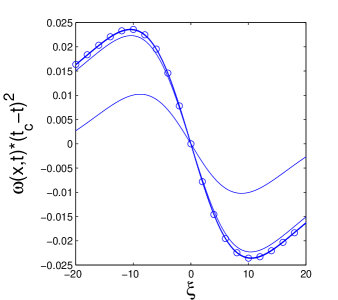
Figure 1: Exact solution of Schochet for $x_{1}(0)=-i$, $x_{2}(0)=-2i$, $\nu=1$, and $K_{+}=24(3+\sqrt{6})$ plotted using similarity variables $\omega(x,t)*(t_{c}-t)^{2}$ versus $\xi$, for $t_{c}-t=10^{-k},k=2,...,7$ (solid cuves). The asymptotic similarity solution (50) is shown by open circles.

Schochet’s exact solution gives self-similar blow up for any initial data. For example, consider his solution with initial data $x_{1}(0)$ and $x_{2}(0)$ on the negative imaginary axis, $0>Im[x_{1}(0)]>Im[x_{2}(0)]$. Then $\omega$ is odd about $x=0$. It is easy to see that the solution for $\omega(x,t)$ blows up at time

$$t_{c}=-\frac{12}{5}\frac{x_{1}(0)x_{2}(0)}{K_{\pm}\nu}$$ (49)

and that the blow up is asymptotically self-similar in a space-time neighborhood of $t=t_{c}$ and $x=0$, i.e., as $x\rightarrow 0$ and $t\rightarrow t_{c}$

$$\omega(x,t)\simeq-\frac{24\tilde{v}}{(t_{c}-t)^{2}}\frac{\xi}{(\xi^{2}+\tilde{v}^{2})^{2}}+O(t_{c}-t)^{-1},$$ (50)

where the similarity variable $\xi$ and $\tilde{v}$ are given by

$$\xi=\frac{x}{t_{c}-t},~{}~{}~{}\tilde{v}=-\frac{5i}{12}\frac{K_{\pm}\nu}{x_{1}(0)+x_{2}(0)}.$$

Figure 1 shows the exact time-dependent solution for $\omega$ with initial singularity positions $x_{1}(0)=-i$,$x_{2}(0)=-2i$ and $\nu=1$. The solution is plotted using similarity variables $\omega(x,t)*(t_{c}-t)^{2}$ versus $\xi=x/(t_{c}-t)$ at the six times $t_{c}-t=10^{-k},k=2,...,7$, and is found to approach a single universal profile. Indeed only three separate profiles are distinguishable, with the four curves for $k=4$ to $7$ that are closest to $t_{c}$ all plotting on top of each other. The open circles show the asymptotic self-similar profile (50) which is approached by the time-dependent solution as $t\rightarrow t_{c}$.

5.2 Exact solution for $a=1/2$ and $\sigma=1$

When $a=1/2$ and $\sigma=1$ a new solution to (LABEL:CLM) is found using the method of pole dynamics. Following the analysis of [31] in the inviscid case $\nu=0$, we look for a solution of the form

$$\omega(x,t)=i\ {\omega_{-2}}(t)\left(\frac{1}{[x-x_{0}-iv_{c}(t)]^{2}}-\frac{1}{[x-x_{0}+iv_{c}(t)]^{2}}\right),$$ (51)

for which

$$u(x,t) ={\omega_{-2}}(t)\left(\frac{1}{x-x_{0}-iv_{c}(t)}+\frac{1}{x-x_{0}+iv_{c}(t)}\right),$$ (52)

$$\mbox{and}~{}~{}\mathcal{H}\omega(x,t) =\ -{\omega_{-2}}(t)\left(\frac{1}{[x-x_{0}-iv_{c}(t)]^{2}}+\frac{1}{[x-x_{0}+iv_{c}(t)]^{2}}\right).$$ (53)

Here $v_{c}$, ${\omega_{-2}}$ and $x_{0}$ are real with $v_{c}>0$ and ${\omega_{-2}}\neq 0$. The vorticity (51) is analytic in a strip $|Im~{}x|<v_{c}(t)$ in the complex plane and has double poles at $x-x_{0}=\pm iv_{c}(t)$. The pure imaginary amplitude $i\ {\omega_{-2}}(t)$ implies that $\omega$ is real and odd for $x\in\mathbb{R}$.

We substitute the ansatz (51) into (LABEL:CLM) (or equivalently the upper analytic component $\omega_{+}$ of (51) into the analog of (41) for $a=1/2$ and $\sigma=1$) and equate like-power poles. Note that the leading order $1/[x-x_{0}\pm iv_{c}(t)]^{4}$ poles cancel out when $a=1/2$, which motivates that choice for $a$ (other choices of $a$ are not consistent with a pole dynamics solution of the form (51)). After multiplication by $(x-x_{0}+iv_{c})\cdot(x-x_{0}-iv_{c})$ we obtain an equation which has only single and double poles with spatially independent coefficients. Setting the coefficients of the double poles to zero gives

$$\frac{dv_{c}(t)}{dt}=-\left(\frac{{\omega_{-2}}(t)}{4v_{c}(t)}-\nu\right).$$ (54)

with initial data $v_{c}(0)>0$. Setting the coefficients of the single poles to zero and using (54) to eliminate $v^{\prime}_{c}(t)$ gives

$$\frac{d{\omega_{-2}}(t)}{dt}=\frac{{\omega_{-2}}^{2}(t)}{4v_{c}^{2}(t)}.$$ (55)

with initial data ${\omega_{-2}}(0)$. Note that (54), (55) reduce to the equations derived in [31] for the inviscid case when $\nu=0$. It is easily verified that (51)-(55) provide an exact solution of the problem (LABEL:CLM) on the real line. In the following we set $\nu=1$, which as noted earlier is equivalent to rescaling $\omega$ and $t$.

It is instructive to define $\Omega={\omega_{-2}}/v_{c}$ and rewrite the system (54)-(55) as

$$\frac{d\Omega}{dt} =\frac{\Omega}{v_{c}}\left(\frac{\Omega}{2}-1\right),$$ (56)

$$\frac{dv_{c}}{dt} =1-\frac{\Omega}{4}.$$ (57)

Clearly, $\Omega(t)=2$ is an unstable equilibrium solution to (56), for which $v_{c}(t)=(t+c)/2$ is the corresponding solution to (57), where $c\in\mathbb{R}$ is an arbitrary constant. In terms of the original variables, this solution is

$$v_{c}(t)=\frac{1}{2}(t+c),~{}{\omega_{-2}}(t)=(t+c),~{}c\in\mathbb{R}~{}\mbox{is a constant}.$$ (58)

A second equilibrium solution to (56) is $\Omega(t)=0$, for which $v_{c}(t)=t+c$ is the corresponding solution to (57). This equilibrium is stable and an attractor for all solutions with data $\Omega(0)<2$.

The above discussion implies that blow up of (51) is determined solely by the sign of the data $\Omega(0)-2$. More precisely, (1) there is finite-time blow up with $v_{c}(t)\rightarrow 0$ when $\Omega(0)>2$, and (2) the solution is analytic and $v_{c}(t)$ is increasing for all $t>0$ when $\Omega(0)\leq 2$.

Straightforward calculations from (51) show that

$$\|\omega(x,t)\|_{L^{\infty}}=\frac{3\sqrt{3}}{4}\frac{\Omega(t)}{v_{c}(t)},\qquad\|\omega(x,t)\|_{L^{2}}=\sqrt{\pi}\frac{\Omega(t)}{\sqrt{v_{c}(t)}}.$$

It is therefore possible to obtain finite-time blow up starting from arbitrarily small data, as measured by either the $L^{2}$ norm or $L^{\infty}$ norm, by taking $\Omega(0)>2$ and $v_{c}(0)\gg 1$.

During blow up ($\Omega(0)>2$), the first term on the right-hand-side of (54) (or equivalently (56)) grows rapidly over time, and the solution asymptotically approaches

$$v_{c}(t)=(t_{c}-t)^{1/3}\widetilde{v}_{c},~{}~{}{\omega_{-2}}(t)=\frac{4\widetilde{v}_{c}^{2}}{3(t_{c}-t)^{1/3}},$$ (59)

in a space-time neighborhood of the singularity $x\rightarrow x_{0}$ and $t\rightarrow t_{c}$, where $\widetilde{v}_{c}>0$ and $t_{c}>0$ are two arbitrary real constants. Numerical solutions illustrating this behavior are shown in Figure 2(a). The vorticity (51) with $v_{c}(t)$ and ${\omega_{-2}}(t)$ given by (59) is an exact solution of the inviscid problem $\nu=0$ [31], and can be written in the self-similar form

$$\omega(x,t)=-\frac{1}{t_{c}-t}\frac{16\tilde{v}_{c}^{3}\xi}{3(\xi^{2}+\tilde{v}_{c}^{2})^{2}},$$ (60)

where

$$\xi=\frac{x-x_{0}}{(t_{c}-t)^{1/3}}.$$

Numerical solutions to (54), (55) in the stable case $\Omega(0)\leq 2$ are shown in Figures 2(b) and (c). These are plotted in the original variables ${\omega_{-2}}$ and $v_{c}$. Figure 2(b) shows the solution for $\Omega(0)=2$ (cf. (58)), while Figure 2(c) shows it for $\Omega(0)=0.5$. In the latter, $\Omega(t)\sim 0$ and $v_{c}(t)\sim t$ for $t\gg 1$, as is verified analytically from (56), (57). Here, the function ${\omega_{-2}}(t)$ tends to a constant as $t\rightarrow\infty$.

Finally, it is noted that we have been able to integrate (56), (57) and obtain a solution in implicit form as

$$\frac{\sqrt{\Omega-2}}{2\Omega}+\frac{1}{2\sqrt{2}}\tan^{-1}\sqrt{\frac{\Omega-2}{2}}=c_{1}t+c_{2}$$ (61)

where $c_{1}$ and $c_{2}$ are constants. While it is not possible to obtain an explicit solution for $\Omega$, the limit $\Omega\rightarrow\infty$ (or equivalently $t\rightarrow t_{c}$) is easily computed with the result that $\Omega(t)\sim(t_{c}-t)^{-2/3}$ in this limit. This gives from (57) that $v_{c}(t)\sim(t_{c}-t)^{1/3}$ and hence $\omega_{-2}(t)\sim(t_{c}-t)^{-1/3}$ when $t\rightarrow t_{c}$. Thus, the similarity scalings for the blow up solution (59) are recovered from the implicit solution (61).

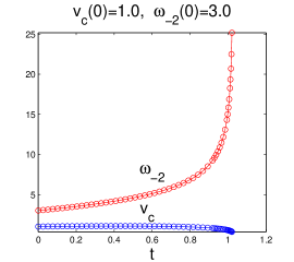
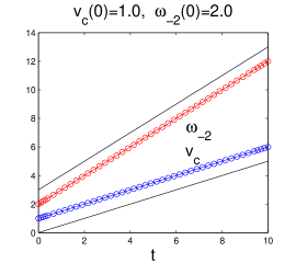
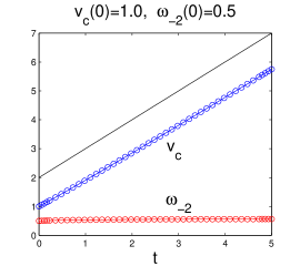
Figure 2: Evolution of ${\omega_{-2}}(t)$ and $v_{c}(t)$ for decreasing $\Omega(0)={\omega_{-2}}(0)/v_{c}(0)$. (a) Finite time blow up for $\Omega(0)=3.0$, (b) Global existence for $\Omega(0)=2.0$, solid lines have slope $1$ and $1/2$, (c) Global existence for $\Omega(0)=0.5$, solid line has slope $1$.

In summary, the analytical solutions derived here for $a=1/2$ and $\sigma=1$ exist globally in time and are smooth (analytic) for initial data $\omega(x,0)$ of the form (51) with $\Omega(0)={\omega_{-2}}(0)/v_{c}(0)\leq 2$. When $\Omega(0)>2$, there is finite-time blow up, and by taking $v_{c}(0)$ large, the blow-up can be made to occur from arbitrarily small data $\|\omega(\cdot,0)\|_{L^{2}}$ or $\|\omega(\cdot,0)\|_{L^{\infty}}$.

5.3 Exact solution for $a=0$ and $\sigma=1$

Another new solution can be found by the method of pole dynamics when $a=0$ and $\sigma=1$. We look for a solution to (LABEL:CLM) in the form of two poles as

$$\omega(x,t)=\frac{\omega_{-1}(t)}{x-\mathrm{i}v_{c}(t)}+\frac{\bar{\omega}_{-1}(t)}{x+\mathrm{i}\bar{v}_{c}(t)}$$ (62)

This is easily seen to result in a solution

$$\omega_{-1}(t)=\omega_{-1}(0),\qquad v_{c}(t)=(\omega_{-1}(0)+\nu)t+v_{c}(0),$$ (63)

where $\omega_{-1}(0)$ and $v_{c}(0)$ are arbitrary complex constants (in contrast to Section 5.2, in which the corresponding constants are real) with $Re[v_{c}(0)]>0$. Note that

(a) If $\omega_{-1}(0)=-\nu$ then the solution (62), (63) is time-independent.

(b) If $Re[\omega_{-1}(0)]>-\nu$ then the solution (62), (63) exists for all $t>0$ because the poles moves away from the real axis.

(c) If $Re[\omega_{-1}(0)]<-\nu$ then the solution (62), (63) exists until $t=t_{c}>0,$ where

$$t_{c}=-\frac{Re[v_{c}(0)]}{Re[\omega_{-1}(0)]+\nu}$$ (64)

is the collapse time (i.e. the time when the poles reach the real axis). Using (62)-(64) we find that at $t=t_{c}$, both poles impinge on the real axis with spatial location given by

$$x=x_{c}:=\mathrm{i}v_{c}(t_{c})=\frac{Im[\omega_{-1}(0)]Re[v_{c}(0)]}{Re[\omega_{-1}(0)]+\nu}-Im[v_{c}(0)]$$ (65)

If $\omega_{-1}(0)\neq-\nu$ then we can rewrite (62)-(65) in a self-similar form

$$\omega(x,t)=\frac{\mathrm{i}}{t_{c}-t}\left(\frac{\xi_{+}+\mathrm{i}\nu}{\xi-\xi_{+}}-\frac{\xi_{-}-\mathrm{i}\nu}{\xi-\xi_{-}}\right),$$ (66)

where

$$\xi_{\pm}=\frac{\pm\mathrm{i}v_{c}(0)-x_{c}}{t_{c}}$$

are positions of poles in the complex plane of $\xi$ and

$$\xi:=\frac{x-x_{c}}{t_{c}-t}$$ (67)

is the self-similar variable. Equation (66) is the analog of equation (30) in [31], which describes self-similar blow up in the inviscid problem. The solution (66) belongs to the general self-similar form (5) with ${\alpha}=\beta=1.$

From (62) we can directly compute norms

$$\|\omega(x,t)\|_{L^{\infty}}=\frac{|\omega_{-1}(t)|+|Im[\omega_{-1}(t)]|}{Re[v_{c}(t)]},\quad\|\omega(x,t)\|_{L^{2}}=\sqrt{2\pi}\frac{|\omega_{-1}(t)|}{\sqrt{Re[v_{c}(t)]}}.$$

Both of the norms can be made arbitrarily small for the initial data of the collapsing solution (66) by choosing $Re[v_{c}(0)]$ large enough.

The solution (62), (63) has infinite kinetic energy $E_{K}(t_{c})$ on the line $x\in\mathbb{R}$ for general values of the parameters $\omega_{-1}(0)$ and $v_{c}(0).$ An exception in which $E_{K}$ is finite occurs for $\omega_{-1}(0)=\bar{\omega}_{-1}(0)$ and $v_{c}(0)=\bar{v}_{c}(0)$, i.e. for purely real values of the residue $\omega_{-1}(0)$ and $v_{c}(0)$ in the solution (62).

We can also consider a solution with two pairs of poles as

$$\omega(x,t)=\frac{\omega_{-1,1}(t)}{x-\mathrm{i}v_{c,1}(t)}+\frac{\bar{\omega}_{-1,1}(t)}{x+\mathrm{i}\bar{v}_{c,1}(t)}+\frac{\omega_{-1,2}(t)}{x-\mathrm{i}v_{c,2}(t)}+\frac{\bar{\omega}_{-1,2}(t)}{x+\mathrm{i}\bar{v}_{c,2}(t)}$$ (68)

in which the poles are located at $x=\mathrm{i}v_{c,1}(t)$, $x=\mathrm{i}v_{c,2}(t)$ and their complex conjugate points. Here we assume that $Re[v_{c,1}(0)]>0$ and $Re[v_{c,2}(0)]>0$. Plugging (68) into (62) and equating the most singular terms (which are proportional to $(x-\mathrm{i}v_{c,1}(t))^{-2}$ and $(x-\mathrm{i}v_{c,2}(t))^{-2}$ at $x=\mathrm{i}v_{c,1}(t)$ and $x=\mathrm{i}v_{c,2}(t)$) results in

$$\frac{dv_{c,1}(t)}{dt}=\nu+\omega_{-1,1}(t)$$ (69)

and

$$\frac{dv_{c,2}(t)}{dt}=\nu+\omega_{-1,2}(t).$$ (70)

Collecting now the next most singular terms which are proportional to $(x-\mathrm{i}v_{c,1}(t))^{-1}$ and $(x-\mathrm{i}v_{c,2}(t))^{-1}$ at $x=\mathrm{i}v_{c,1}(t)$ and $x=\mathrm{i}v_{c,2}(t)$ results in

$$\frac{d\omega_{-1,1}(t)}{dt}=\frac{2\omega_{-1,1}(t)\omega_{-1,2}(t)}{v_{c,1}(t)-v_{c,2}(t)}$$ (71)

and

$$\frac{d\omega_{-1,2}(t)}{dt}=\frac{2\omega_{-1,1}(t)\omega_{-1,2}(t)}{v_{c,2}(t)-v_{c,1}(t)}=-\frac{d\omega_{-1,1}(t)}{dt}.$$ (72)

Substitution of (68)-(72) into the governing equations (LABEL:CLM) reveals that they are identically satisfied. A solution of the system (69)-(72) follows from the observation that $\frac{d\omega_{-1,2}(t)}{dt}=-\frac{d\omega_{-1,1}(t)}{dt}$ from (71),(72), so that

$$c_{0}:=\omega_{-1,1}(t)+\omega_{-1,2}(t)=\omega_{-1,1}(0)+\omega_{-1,2}(0).$$ (73)

Together with (69),(70), this implies that $\frac{d[v_{c,1}(t)+v_{c,2}(t)]}{dt}=2\nu+c_{0},$ i.e. $v_{c,2}(t)=-v_{c,1}(t)+(2\nu+c_{0})t+v_{c,1}(0)+v_{c,2}(0)$. Thus we reduce the system (69)-(72) from four ordinary differential equations (ODEs) to two ODEs for $v_{c,1}(t)$ and $\omega_{-1,1}(t)$, which is easily solved. The solution of the system (69)-(72) for $c_{0}\neq 0$ is

$$\begin{split}&\omega_{-1,1}(t)=\frac{c_{0}}{2}+\frac{1}{2}\frac{c_{1}+\frac{c_{0}^{2}t}{v_{c,1}(0)-v_{c,2}(0)}}{\sqrt{1+\frac{2c_{1}t}{v_{c,1}(0)-v_{c,2}(0)}+\frac{c_{0}^{2}t^{2}}{(v_{c,1}(0)-v_{c,2}(0))^{2}}}},\\ &\omega_{-1,2}(t)=-\omega_{-1,1}(t)+c_{0},\\ &v_{c,1}(t)=\frac{c_{0}}{2}t+\nu t+\frac{v_{c,1}(0)-v_{c,2}(0)}{2}\sqrt{1+\frac{2c_{1}t}{v_{c,1}(0)-v_{c,2}(0)}+\frac{c_{0}^{2}t^{2}}{(v_{c,1}(0)-v_{c,2}(0))^{2}}}+\\ &+\frac{v_{c,1}(0)+v_{c,2}(0)}{2},\\ &v_{c,2}(t)=-v_{c,1}(t)+(2\nu+c_{0})t+v_{c,1}(0)+v_{c,2}(0),\end{split}$$

where $c_{0}$ is given by Eq. (73), $c_{1}:=\omega_{-1,1}(0)-\omega_{-1,2}(0)$, and we assumed a principle branch of the square root.

For $c_{0}=0$, when $\omega_{-1,1}(0)=-\omega_{-1,2}(0)$, the solution of the system (69)-(72) is

$$\begin{split}&\omega_{-1,1}(t)=-\omega_{-1,2}(t)=\frac{\omega_{-1,1}(0)}{\sqrt{1+\frac{4\omega_{-1,1}(0)t}{v_{c,1}(0)-v_{c,2}(0)}}},\\ &v_{c,1}(t)=\nu t+\frac{v_{c,1}(0)-v_{c,2}(0)}{2}\sqrt{1+\frac{4\omega_{-1,1}(0)t}{v_{c,1}(0)-v_{c,2}(0)}}+\frac{v_{c,1}(0)+v_{c,2}(0)}{2},\\ &v_{c,2}(t)=-v_{c,1}(t)+2\nu t+v_{c,1}(0)+v_{c,2}(0).\\ \end{split}$$ (74)

The above solutions develop a finite-time singularity on the real line of $x$ at $t=t_{c}$ provided $Re[v_{c,1}(t_{c})]=0$ or $Re[v_{c,2}(t_{c})]=0$. By relabeling complex singularities if necessary, we can assume without loss of generality that $x=\mathrm{i}v_{c,1}(t)$ reaches the real line first (ahead of $x=\mathrm{i}v_{c,2}(t))$ thus resulting in collapse. (It remains an open question whether it is possible to have $v_{c,1}(t_{c})=v_{c,2}(t_{c})$, thus creating a higher order singularity at $t=t_{c}.$) Then for $t\to t_{c}-$ and in a small spatial neighborhood of $x=\mathrm{i}v_{c,1}(t_{c})$, the solution (68) is dominated by singularities at $x=\mathrm{i}v_{c,1}(t)$ and $x=-\mathrm{i}\bar{v}_{c,1}(t)$, so that (68) reduces to

$$\omega(x,t)\simeq\frac{\omega_{-1,1}(t)}{x-\mathrm{i}v_{c,1}(t)}+\frac{\bar{\omega}_{-1,1}(t)}{x+\mathrm{i}\bar{v}_{c,1}(t)}.$$ (75)

Generically the singularity at $t=t_{c}$ located at $x=\mathrm{i}v_{c,1}(t)$ hits the real line $Im(x)=0$ with a nonzero vertical velocity $\left.\frac{dRe[v_{c,1}(t)]}{dt}\right|_{t=t_{c}}<0.$ Then for $t\to t_{c}-$ the solution (75) can be further reduced using the Taylor series approximation $v_{c,1}(t)=\mathrm{i}Im[v_{c,1}(t_{c})]+v_{c,1}^{\prime}(t_{c})(t-t_{c})+O(t-t_{c})^{2}$ (here $v_{c,1}^{\prime}(t_{c}):=\frac{dv_{c,1}(t_{c})}{dt}$) and neglecting the $O(t-t_{c})^{2}$ term. We also assume that $\omega_{-1,1}(t_{c})\neq 0$ and replace $\omega_{-1,1}(t)$ by $\omega_{-1,1}(t_{c})$ to obtain from (75)

$$\omega(x,t)\simeq\frac{\omega_{-1,1}(t_{c})}{x+Im[v_{c,1}(t_{c})]-\mathrm{i}(t-t_{c})v_{c,1}^{\prime}(t_{c})}+\frac{\bar{\omega}_{-1,1}(t_{c})}{x+Im[v_{c,1}(t_{c})]+\mathrm{i}(t-t_{c})\bar{v}_{c,1}^{\prime}(t_{c})}.$$

This has the self-similar form (5) with $\alpha=\beta=1$.

A special situation occurs when $Re[v_{c,1}^{\prime}(t_{c})]=0.$ In that case $v_{c,1}^{\prime}(t)=\mathrm{i}Im[v_{c,1}^{\prime}(t_{c})]+O(t_{c}-t)$, which corresponds to the pole singularity hitting the real line of $x$ with vanishing vertical velocity. In that case equation (75) turns into

$$\omega(x,t)\simeq\frac{\omega_{-1,1}(t_{c})}{x+Im[v_{c,1}(t_{c})]+Im[v_{c,1}^{\prime}(t_{c})](t-t_{c})-\frac{\mathrm{i}}{2}(t-t_{c})^{2}v_{c,1}^{\prime\prime}(t_{c})}+\\ \frac{\bar{\omega}_{-1,1}(t_{c})}{x+Im[v_{c,1}(t_{c})]+Im[v_{c,1}^{\prime}(t_{c})](t-t_{c})+\frac{\mathrm{i}}{2}(t-t_{c})^{2}\bar{v}^{\prime\prime}_{c,1}(t_{c})}.$$ (76)

This occurs, for example, when $\omega_{-1,1}(0)=-\omega_{-1,2}(0)=K$, where $K<0$ is a real number, and

$$\frac{Re[v_{c,2}(0)]}{Re[v_{c,1}(0)]}=\left(\frac{K-\nu}{K+\nu}\right)^{2},Im[v_{c,1}(0)]=Im[v_{c,2}(0)]=0.$$

In this case, $t_{c}=\frac{K^{2}-\nu^{2}}{4K\nu^{2}}Re[v_{c,2}(0)-v_{c,1}(0)]$.

Interestingly, the solution (76) has a different self-similar scaling than (66),(67), with $\alpha=\beta=2.$ Direct numerical simulations in Section 7.3.3 show this type of self-similar collapse is unstable to perturbations, as might be expected.

The solution (68), similar to (62), may have arbitrarily small $L^{\infty}$ and $L^{2}$ norms at $t=0$ if we choose $Re[v_{c,1}(0)]$ and $Re[v_{c,2}(0)]$ large enough. These norms simplify in the case $Im[v_{c,1}(0)]=Im[v_{c,2}(0)]=0$, e.g., in which

$$\|\omega(x,t)\|_{L^{2}}=\\ \sqrt{2\pi}\sqrt{\frac{|\omega_{-1,1}(t)|^{2}}{v_{c,1}(t)}+\frac{|\omega_{-1,2}(t)|^{2}}{v_{c,2}(t)}+\frac{4(Re[\omega_{-1,1}(t)]Re[\omega_{-1,2}(t)]+Im[\omega_{-1,1}(t)]Im[\omega_{-1,2}(t)])}{v_{c,1}(t)+v_{c,2}(t)}}.$$ (77)

5.4 Exact solution for $a=0$ and $\sigma=0$

Another solution can be found by the method of pole dynamics when $a=0$ and $\sigma=0$. In this case ${\Lambda}^{0}(\omega)=\omega$. We look for a solution to (LABEL:CLM) in the form of two simple poles as

$$\omega(x,t)=\frac{\omega_{-1}(t)}{x-\mathrm{i}v_{c}(t)}+\frac{\bar{\omega}_{-1}(t)}{x+\mathrm{i}\bar{v}_{c}(t)},$$ (78)

where $\omega_{-1}(0)$ and $v_{c}(0)$ are arbitrary complex constants with $Re[v_{c}(0)]>0$.

From (78) we directly compute norms

$$\|\omega(x,t)\|_{L^{\infty}}=\frac{|\omega_{-1}(t)|+|Im[\omega_{-1}(t)]|}{Re[v_{c}(t)]},\quad\|\omega(x,t)\|_{L^{2}}=\sqrt{2\pi}\frac{|\omega_{-1}(t)|}{\sqrt{Re[v_{c}(t)]}}.$$

Substituting (78) into (LABEL:CLM) we get the following equations:

$$\frac{d\omega_{-1}(t)}{dt}=-\nu\omega_{-1}(t),\qquad\frac{dv_{c}(t)}{dt}=\omega_{-1}(t),$$

and their solution:

$$\omega_{-1}(t)=\omega_{-1}(0)e^{-\nu t},\qquad v_{c}(t)=\frac{\omega_{-1}(0)}{\nu}(1-e^{-\nu t})+v_{c}(0),$$ (79)

which for $\nu=0$ reduces to

$$\omega_{-1}(t)=\omega_{-1}(0),\qquad v_{c}(t)=\omega_{-1}(0)t+v_{c}(0).$$ (80)

For the case $\nu=0$ we always have a collapsing solution (even for arbitrarily small data in $L^{\infty}$ and $L^{2}$ norms) if $Re[\omega_{-1}(0)]<0$, since $Re[v_{c}(t_{c})]=0$ at $t_{c}=\frac{Re[v_{c}(0)]}{-Re[\omega_{-1}(0)]}$. This solution is equivalent to (32) in [31], which describes self-similar blow up in the inviscid problem.

Note that for $\nu>0$ equations (79) indicate either global existence of the solution (78) or a collapsing solution depending on initial values of $\omega_{-1}(0)$ and $v_{c}(0)$:

(a) If $Re[\omega_{-1}(0)]>-\nu Re[v_{c}(0)]$ then $Re[v_{c}(t)]>0$ for all $t>0$ and the solution (78), (79) exists for any $t>0$.

(b) If $Re[\omega_{-1}(0)]=-\nu Re[v_{c}(0)]$ then $Re[v_{c}(t)]=Re[v_{c}(0)]e^{-\nu t}\rightarrow 0$ as $t\rightarrow\infty$, and the solution (78), (79) exists for all $t>0$ because the poles approach the real axis exponentially in time. They approach the real line at the point

$$x=x_{c}:=Re[iv_{c}(\infty)]=-Im[v_{c}(\infty)]=-\frac{Im[\omega_{-1}(0)]}{\nu}-Im[v_{c}(0)],$$ (81)

and $\|\omega(x,t)\|_{L^{\infty}}=\|\omega(x,0)\|_{L^{\infty}}=const>0$, $\|\omega(x,t)\|_{L^{2}}\sim e^{-\nu t/2}\rightarrow 0$ as $t\rightarrow\infty$.

(c) If $Re[\omega_{-1}(0)]<-\nu Re[v_{c}(0)]$ then the solution (78), (79) exists until the collapse time

$$t_{c}=-\frac{1}{\nu}\ln\left(1+\frac{\nu Re[v_{c}(0)]}{Re[\omega_{-1}(0)]}\right),$$ (82)

at which the poles reach the real axis. Here $\|\omega(x,t)\|_{L^{\infty}},\|\omega(x,t)\|_{L^{2}}\rightarrow\infty$ as $t\rightarrow t_{c}$ since $\omega_{-1}(t_{c})\neq 0$ and $Re[v_{c}(t_{c})]=0$. Crucially, collapse occurs even when the initial norm $\|\omega(x,0)\|_{L^{2}}$ is made arbitrarily small by taking small $v_{c}(0)$. In contrast, $\|\omega(x,0)\|_{L^{\infty}}>\nu$, i.e., the $L^{\infty}$ norm is bounded from below.

Using (79)-(82) we find that at $t=t_{c}$, both poles cross the real axis at the location

$$x=x_{c}:=\mathrm{i}v_{c}(t_{c})=-Im[v_{c}(t_{c})]=\frac{Im[\omega_{-1}(0)]}{Re[\omega_{-1}(0)]}Re[v_{c}(0)]-Im[v_{c}(0)],$$

with the complex velocity of the first pole being

$$v_{c}^{\prime}(t_{c})=\omega_{-1}(t_{c})=\omega_{-1}(0)e^{-\nu t_{c}}=\omega_{-1}(0)\left(1+\frac{\nu Re[v_{c}(0)]}{Re[\omega_{-1}(0)]}\right).$$

Since $v_{c}(t_{c})=\mathrm{i}Im[v_{c}(t_{c})]$, we have that in a space-time neighborhood of the singularity $x\rightarrow x_{c}$ and $t\rightarrow t_{c}$ the solution (79) asymptotically approaches

$$\omega_{-1}(t)=\omega_{-1}(t_{c})+O(t_{c}-t),v_{c}(t)=\mathrm{i}Im[v_{c}(t_{c})]-\omega_{-1}(t_{c})(t_{c}-t)+O(t_{c}-t)^{2},$$

and the solution (78) can be written in a self-similar form

$$\omega(x,t)=\frac{\mathrm{i}}{t_{c}-t}\left(\frac{\xi_{+}}{\xi-\xi_{+}}-\frac{\xi_{-}}{\xi-\xi_{-}}\right)+O(1),$$ (83)

where

$$\xi_{+}=-\mathrm{i}\omega_{-1}(t_{c}),\quad\xi_{-}=\mathrm{i}\bar{\omega}_{-1}(t_{c}),$$

are positions of poles in the complex plane of $\xi$ and

$$\xi:=\frac{x-x_{c}}{t_{c}-t}$$

is the self-similar variable. Equation (83) is a viscous analog of equation (30) in [31], which describes self-similar blow up in the inviscid problem. The solution (83) belongs to the general self-similar form (5) with $\alpha=\beta=1.$

The kinetic energy $E_{K}(t)=\int u^{2}(x,t)dx$ in (a), (b) scales like $E_{K}(t)\sim e^{-2\nu t}$ as $t\rightarrow\infty$, whereas in (c) $E_{K}(t_{c})$ is finite for any complex values of the parameters $\omega_{-1}(0)$ and $v_{c}(0)$, in contrast to the $a=0,\sigma=1$ case.

6 Exact solution to the periodic problem for     $a=0$ and $\sigma=0$

In this section we adapt the analysis of Section 5.4 to obtain an exact analytical solution in the periodic geometry. We take $a=0$, $\sigma=0$, $\nu>0$, in which case (7) becomes

$$\omega_{t}=\omega\mathcal{H}(\omega)-\nu\omega.$$ (84)

We take initial data with zero mean value on $x\in[-\pi,\pi]$, which is then preserved under the evolution.

Using the Hilbert transform representation (8) we can rewrite (84) as:

$$\omega_{-t}=\mathrm{i}\omega_{-}^{2}-\nu\omega_{-},$$ (85)

where $\omega_{-}$ is analytic in the lower half-plane $\mathbb{C}^{-}$. We look for a solution to (85) in the form of a single pole in $\tan(\frac{x}{2})$-space:

$$\omega_{-}(x,t)=\omega_{-1}(t)\left[\frac{1}{\tan(\frac{x}{2})-\mathrm{i}v_{c}(t)}-\frac{1}{-\mathrm{i}-\mathrm{i}v_{c}(t)}\right],$$ (86)

where $\omega_{-1}(0)$ and $v_{c}(0)$ are arbitrary complex constants with $Re[v_{c}(0)]>0$. The term $\frac{1}{-\mathrm{i}-\mathrm{i}v_{c}(t)}$ is subtracted so that $\omega_{-}(x,t)$ has zero mean value on $x\in[-\pi,\pi]$, $\int_{-\pi}^{\pi}{\omega_{-}(x,t)dx}=0$. We supplement $\omega_{-}(x,t)$ from (86) with $\omega_{+}(x,t)=\overline{\omega_{-}(\bar{x},t)}$ to get a real-valued solution $\omega=\omega_{-}+\omega_{+}$ of (84).

From (86) we compute norms

$$\|\omega(x,t)\|_{L^{\infty}}=\frac{|\omega_{-1}(t)|-Im[\omega_{-1}(t)]}{Re[v_{c}(t)]}+2\frac{Im[\omega_{-1}(t)](1+Re[v_{c}(t)])-Im[v_{c}(t)]Re[\omega_{-1}(t)]}{(Im[v_{c}(t)])^{2}+(1+Re[v_{c}(t)])^{2}},\\ \|\omega(x,t)\|_{L^{2}}=2\sqrt{\pi}\frac{|\omega_{-1}(t)|}{\sqrt{Re[v_{c}(t)]((Im[v_{c}(t)])^{2}+(1+Re[v_{c}(t)])^{2})}},\\ \|\omega(x,t)\|_{B_{0}}=\frac{|\omega_{-1}(t)|}{Re[v_{c}(t)]}\left(\sqrt{\frac{(Im[v_{c}(t)])^{2}+(1-Re[v_{c}(t)])^{2}}{(Im[v_{c}(t)])^{2}+(1+Re[v_{c}(t)])^{2}}}+1\right).$$ (87)

Substituting (86) to (85) we get the following equations:

$$\frac{d\omega_{-1}(t)}{dt}=-\nu\omega_{-1}(t)+\frac{2\omega_{-1}^{2}(t)}{1+v_{c}(t)},\qquad\frac{dv_{c}(t)}{dt}=\omega_{-1}(t),$$

and their solution:

$$\omega_{-1}(t)=\omega_{-1}(0)e^{-\nu t}\left(\frac{1-e^{-\nu t_{0}}}{1-e^{-\nu(t+t_{0})}}\right)^{2},v_{c}(t)=\frac{\omega_{-1}(0)}{\nu}\frac{(1-e^{-\nu t_{0}})(1-e^{-\nu t})}{1-e^{-\nu(t+t_{0})}}+v_{c}(0),$$ (88)

where $e^{\nu t_{0}}=1-\frac{\nu(1+v_{c}(0))}{\omega_{-1}(0)}$ is complex valued in general.

Equations (88) for $\nu=0$ reduce to:

$$\omega_{-1}(t)=\frac{\omega_{-1}(0)}{(1-\frac{\omega_{-1}(0)}{1+v_{c}(0)}t)^{2}},\qquad v_{c}(t)=\frac{v_{c}(0)+\frac{\omega_{-1}(0)}{1+v_{c}(0)}t}{1-\frac{\omega_{-1}(0)}{1+v_{c}(0)}t}.$$ (89)

For the case $\nu=0$ we always have a collapsing solution (even for arbitrarily small data) at $t=t_{c}$ with collapse location

$$x=x_{c}=2\tan^{-1}(\mathrm{i}v_{c}(t_{c}))=2\tan^{-1}(-Im[v_{c}(t_{c})]),$$ (90)

since $v_{c}(\infty)=-1<0$ for any $\omega_{-1}(0)$.

We have $Re[v_{c}(t_{c})]=0$ at time

$$t_{c}=\frac{X+\sqrt{4|\omega_{-1}(0)|^{2}Re[v_{c}(0)](|v_{c}(0)|^{2}+1+2Re[v_{c}(0)])+X^{2}}}{2|\omega_{-1}(0)|^{2}},$$ (91)

$$X=Re[\omega_{-1}(0)](1+Im[v_{c}(0)]^{2}-Re[v_{c}(0)]^{2})-2Im[\omega_{-1}(0)]Im[v_{c}(0)]Re[v_{c}(0)].$$

For purely real $v_{c}(0)$ and $\omega_{-1}(0)$ equations (91) and (90) reduce to

$$t_{c} =-\frac{v_{c}(0)(1+v_{c}(0))}{\omega_{-1}(0)}, x_{c}=0 \mbox{for}\quad\omega_{-1}(0)<0,$$

$$t_{c} =\frac{1+v_{c}(0)}{\omega_{-1}(0)}, x_{c}=\pm\pi \mbox{for}\quad\omega_{-1}(0)>0.$$

The solution (86), (89) is a periodic analog of equation (32) in [31], which describes self-similar blow up in the inviscid problem. The solution (86) with $\omega(x,t)=\omega_{-}(x,t)+\overline{\omega_{-}(\bar{x},t)}$ belongs to the general self-similar form (5) with $\alpha=\beta=1.$

When $\nu>0$ the same analysis as (a)-(c) in Section 5.4 can be done. In this case (88) gives either global existence of the solution (86) or a collapsing solution depending on initial values of $\omega_{-1}(0)$ and $v_{c}(0)$. For simplicity, we assume that $\omega_{-1}(0)$ and $v_{c}(0)$ are purely real. Then (87) becomes

$$\|\omega(x,t)\|_{L^{\infty}} =\frac{|\omega_{-1}(t)|}{v_{c}(t)},\qquad\;\;\,\|\omega(x,t)\|_{L^{2}}=2\sqrt{\pi}\frac{|\omega_{-1}(t)|}{\sqrt{v_{c}(t)}(1+v_{c}(t))},$$

$$\|\omega(x,t)\|_{B_{0}} =\frac{|\omega_{-1}(t)|}{v_{c}(t)}\left(\frac{|1-v_{c}(t)|}{1+v_{c}(t)}+1\right).$$ (92)

Rewriting the second equation of (88) we get

$$v_{c}(t)=\frac{\omega_{-1}(0)(1-e^{-\nu t})+\nu v_{c}(0)(1+v_{c}(0))}{-\omega_{-1}(0)(1-e^{-\nu t})+\nu(1+v_{c}(0))},$$

from which we can conclude that:

(a) If $-\nu v_{c}(0)(1+v_{c}(0))<\omega_{-1}(0)<\nu(1+v_{c}(0))$ then $0<v_{c}(t)<\infty$ for all $t>0$ and the solution (86), (88) exists for any $t>0$.

(b1) If $\omega_{-1}(0)=-\nu v_{c}(0)(1+v_{c}(0))$ then $\omega_{-1}(t),v_{c}(t)\sim e^{-\nu t}\rightarrow 0$ as $t\rightarrow\infty$, and the solution (86), (88) exists for all $t>0$ because the poles approach the real line at $x_{c}=0$ exponentially in time.

(b2) If $\omega_{-1}(0)=-\nu(1+v_{c}(0))$ then $\omega_{-1}(t),v_{c}(t)\sim e^{\nu t}\rightarrow\infty$ as $t\rightarrow\infty$, and the solution (86), (88) exists for all $t>0$ because the poles approach the real line at $x_{c}=2\tan^{-1}(\mathrm{i}\infty)=\pm\pi$ exponentially in time.

In both (b1) and (b2) cases $\|\omega(x,t)\|_{L^{\infty}},\|\omega(x,t)\|_{B_{0}}/2\rightarrow\nu>0$, $\|\omega(x,t)\|_{L^{2}}\sim e^{-\nu t/2}\rightarrow 0$ as $t\rightarrow\infty$.

(c1) If $\omega_{-1}(0)<-\nu v_{c}(0)(1+v_{c}(0))$ then the solution (86), (88) exists until the collapse time $t_{c}$ (when the poles reach the real axis at $v_{c}(t_{c})=0$, $x_{c}=0$), where

$$t_{c}=\frac{1}{\nu}\ln\left(\frac{\omega_{-1}(0)}{\omega_{-1}(0)+\nu v_{c}(0)(1+v_{c}(0))}\right).$$

Using (6), we get that blow up occurs for any initial data satisfying

$$\|\omega(x,0)\|_{L^{\infty}}>\nu(1+v_{c}(0))>\nu, \|\omega(x,0)\|_{L^{2}}>2\nu\sqrt{\pi v_{c}(0)},$$

$$\|\omega(x,0)\|_{B_{0}}>2\nu,\mbox{ if }v_{c}(0)<1, \|\omega(x,0)\|_{B_{0}}>2\nu v_{c}(0),\mbox{ if }v_{c}(0)\geq 1.$$

We therefore see that $\|\omega(x,0)\|_{L^{2}}$ can be made arbitrarily small by choosing small enough $v_{c}(0)$, but $\|\omega(x,0)\|_{L^{\infty}}$ and $\|\omega(x,0)\|_{B_{0}}$ cannot be made similarly small.

(c2) If $\omega_{-1}(0)>\nu(1+v_{c}(0))$ then the solution (86), (88) exists until the collapse time $t_{c}$ (when the poles reach the real axis at $v_{c}(t_{c})=\infty$, $x_{c}=\pm\pi$), where

$$t_{c}=\frac{1}{\nu}\ln\left(\frac{\omega_{-1}(0)}{\omega_{-1}(0)-\nu(1+v_{c}(0))}\right).$$

Using (6), we get that blow up occurs for any initial data satisfying

$$\|\omega(x,0)\|_{L^{\infty}}>\nu\left(1+\frac{1}{v_{c}(0)}\right)>\nu, \|\omega(x,0)\|_{L^{2}}>2\nu\sqrt{\frac{\pi}{v_{c}(0)}},$$

$$\|\omega(x,0)\|_{B_{0}}>2\frac{\nu}{v_{c}(0)},\mbox{ if }v_{c}(0)<1, \|\omega(x,0)\|_{B_{0}}>2\nu,\mbox{ if }v_{c}(0)\geq 1,$$

We again see that $\|\omega(x,0)\|_{L^{2}}$ (but not $\|\omega(x,0)\|_{L^{\infty}}$ and $\|\omega(x,0)\|_{B_{0}}$) can be made arbitrarily small by choosing large enough $v_{c}(0)$.

In both (c1) and (c2), the collapse is self-similar and the solution (86) together with $\omega(x,t)=\omega_{-}(x,t)+\overline{\omega_{-}(\bar{x},t)}$ belongs to the general self-similar form (5) with $\alpha=\beta=1$ and $\|\omega(x,t)\|_{L^{\infty}},\|\omega(x,t)\|_{L^{2}}\rightarrow\infty$ as $t\rightarrow t_{c}$, since in (c1) $\omega_{-1}(t_{c})\neq 0$ and $v_{c}\sim(t_{c}-t)$, in (c2) $\omega_{-1}\sim(t_{c}-t)^{-2}$ and $v_{c}\sim(t_{c}-t)^{-1}$.

Similarly to the real line solution, the kinetic energy $E_{K}(t)=\int u^{2}(x,t)dx$ in (a), (b1), (b2) scales like $E_{K}(t)\sim e^{-2\nu t}$ as $t\rightarrow\infty$, whereas in (c1), (c2) $E_{K}(t_{c})$ is finite for any complex values of the parameters $\omega_{-1}(0)$ and $v_{c}(0)$.

Similar exact solutions can be derived with one pair of simple poles in $\tan(\frac{x}{2})$-space for $a=0,~{}\sigma=1$, and one pair of double poles for $a=1/2,~{}\sigma=0,1$, as periodic analogues of exact solutions on the real line. Details are left for future work.

7 Numerical results

We present the results of direct time-dependent numerical simulations of (LABEL:CLM) in both the periodic and real-line geometries. The numerical results are consistent with the analytical theory on global existence for small data in the periodic setting, and further indicate that finite-time singularities can form for sufficiently large data. They also are in quantitative agreement with with the exact solutions presented in Sections 5 and 6, and give information on the stability of those solutions.

7.1 Numerical method

We provide a brief description of the numerical method and the procedure for tracking complex singularities. More details are given in [31]. In the periodic case, (LABEL:CLM) is numerically solved for $x\in\mathbb{S}=[\-\pi,\pi]$ using a pseudo-spectral Fourier method based on the representation

$$\omega(x,t)=\sum_{k=-N}^{N-1}\hat{\omega}_{k}(t)e^{ikx}$$

in terms of $2N$ Fourier modes. Derivatives along with the periodic Hilbert transform and the dissipation term are computed by wavenumber multiplication in Fourier space. Time stepping is performed using an 11-stage explicit Runge-Kutta method of $8th$ order [12] with adaptive time step determined by the condition $\Delta t=CFL\cdot\min[\Delta x/(a\max_{x}|u(x,t)|),1/\max_{x}|u_{x}(x,t)|,(\Delta x)^{\sigma}/\nu]$, where $\Delta x=\pi/N$ and the numerical constant $CFL$ is chosen as $1/16,1/32$ or $1/64$. This condition ensures numerical stability and that the error in time-stepping is near round-off.

The decay of the Fourier spectrum is checked at the end of every time step, and if $|\omega_{k}(t)|$ is larger than numerical round-off at $|k|\sim N$, the simulation is “rewound” one time step backward, $N$ increased by a factor of $2$ via zero padding (i.e., Fourier interpolation), and the time step is adjusted before time-stepping is continued. Rewinding helps avoid accumulation of error from the tails of the spectrum not being fully resolved.

To compute on the infinite domain, we make a change of variable

$$x=\tan\left(\frac{q}{2}\right),$$ (93)

which maps $(-\pi,\pi)$ in $q$ to $(-\infty,\infty)$ in $x$. The transformed equations are [31]

$$\begin{split}&\omega_{t}=-a(1+\cos{q})u\omega_{q}+\omega[{\mathcal{H}}^{q}\omega+C_{\omega}^{q}]-\nu[(1+\cos q)\partial_{q}\mathcal{H}^{q}]^{\sigma}\omega,\\ &(1+\cos{q})u_{q}=[{\mathcal{H}}^{q}\omega+C_{\omega}^{q}],~{}~{}q\in(-\pi,\pi),\end{split}$$ (94)

where $\mathcal{H}^{q}$ is the periodic Hilbert transform in $q$

$${\mathcal{H}}^{q}f(q)=\frac{1}{2\pi}PV\int_{-\pi}^{\pi}f(q^{\prime})\cot\left(\frac{q-q^{\prime}}{2}\right)\ dq^{\prime},$$

and the constant $C_{\omega}^{q}$ is determined by

$$C_{\omega}^{q}=-\frac{1}{2\pi}\int^{\pi}_{-\pi}\omega(q^{\prime})\tan(\frac{q^{\prime}}{2})\mbox{d}q^{\prime},$$

so that ${\mathcal{H}}^{q}\omega(\pm\pi)+C_{\omega}^{q}=0$.

A pseudo-spectral method similar to that used for the periodic case is then employed to solve (94), using the Fourier representation in $q$ space

$$\omega(q,t)=\sum_{k=-N}^{N-1}\hat{\omega}_{k}(t)e^{ikq}$$

and a modified adaptive time-step condition $\Delta t=CFL\cdot\min[\Delta q/(a\max_{q}|(1+\cos q)u(q,t)|),1/\max_{q}|(1+\cos q)u_{q}(q,t)|,\max_{q}|\omega(q,t)|/\max_{q}|\nu[(1+\cos q)\partial_{q}\mathcal{H}]^{\sigma}\omega(q,t)|]$. We only consider cases in which $\sigma$ is a non-negative integer, so that the dissipation term can be easily computed by wavenumber multiplication in Fourier space.

Two complementary methods are employed to detect singularities in the complex plane. The first method uses a least squares fit of the asymptotic Fourier decay

$$|\hat{\omega}_{k}(t)|\approx C(t)\frac{e^{-\delta(t)|k|}}{|k|^{p(t)}}$$ (95)

for $|k|\gg 1$ [6], where $C(t),\delta(t)>0$ and $p(t)$ are fitting parameters. The value of $\delta(t)$ gives the distance at time $t$ of the (single) closest complex singularity in $\omega$ to the real line, and $p(t)$ is related to the type or power of singularity. If the closest singularity to the real line has the power law form $(q-q_{c})^{-\gamma}$, then $\delta=|Im(q_{c})|$ and $p=1-\gamma$. On the infinite domain with the additional transform (93), the fitting (95) provides the distance of the closest complex singularity of $\omega$ to the real line in $q$-space. To find the the distance to the closest singularity in $x$-space, we use $\delta_{x}=\tanh(\delta/2)$, when $|Re(q_{c})|=0$ and $\delta_{x}=\coth(\delta/2)$, when $|Re(q_{c})|=\pm\pi$.

This type of Fourier fitting procedure for tracking complex singularities was originally proposed by Sulem et al. [41] and extended in [3], [35]. For more details about the version employed here, see [31].

The second method for detecting complex singularities makes use of analytical continuation based on rational interpolants. Specifically, we employ a modified version of the AAA algorithm originally due to Nakatsukasa et al. [32]. This has the advantage of providing a structure of complex singularities beyond the one closest to the real line, although $|Im(q_{c})|$ and $\gamma$ can be determined more accurately by Fourier fitting than via the AAA algorithm. See Section 10 of [31] for more details on the AAA algorithm employed here.

7.2 Periodic problem

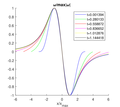
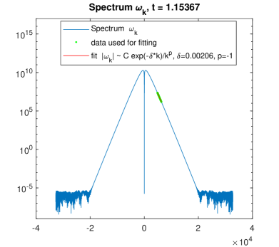
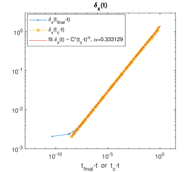
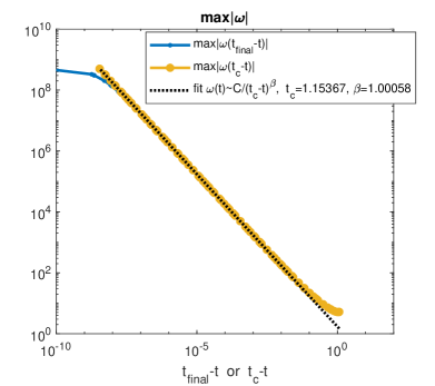
Figure 3: Evolution of the collapsing periodic solution with parameters $a=1/2$, $\sigma=1$, $\nu=1$ and two-mode initial data (96) with $A=4$. Top-left: Scaled solution $\omega(x/|x_{max}|)/\max_{x}|\omega|$ versus $x/|x_{max}|$ (where $x_{max}>0$ is the location of $\max_{x}|\omega|$) at different times in the evolution. Top-right: Spectrum $\log|{\hat{\omega}}_{k}|$ versus $k$ at $t=1.1536657$ and fit by (95). Bottom-left: Log-log plot of $\delta_{x}(t)=\delta(t)$, the distance of the closest singularity to the real line, versus $t_{final}-t$ (in blue) and $t_{c}-t$ (in yellow) and fit to $\delta_{x}(t)\sim C(t_{c}-t)^{\alpha},\alpha\approx 1/3$. Bottom-right: Log-log plot of $\max_{x}|\omega|$ versus $t_{c}-t$ and the fit $\max_{x}|\omega|(t)\sim C/(t_{c}-t)^{\beta},t_{c}\approx 1.15367,\beta\approx 1$.

Figure 3 gives an illustrative example of finite-time collapse in the case of the periodic problem with parameter values $a=1/2$, $\sigma=1$ and $\nu=1$, for two-mode initial data

$$\omega_{0}(x)=\mathrm{i}A\left(\frac{1}{(\tan(\frac{x}{2})-\mathrm{i})^{2}}-\frac{1}{(\tan(\frac{x}{2})+\mathrm{i})^{2}}\right)=-A(\sin x+\sin(2x)/2).$$ (96)

The top-left panel plots a scaled solution $\omega(x/|x_{max}|)/\max_{x}|\omega|$ versus $x/|x_{max}|$ at different times in the evolution. The solution curves approach a universal self-similar profile $f(\xi)$ in a space-time neighborhood of the collapse point. This verifies the self-similar nature of the collapse. The top-right panel show the spectrum $\hat{\omega}_{k}$ of the solution at $t=1.1536657$ and fit by (95). We choose an interval of $k$ somewhere between $1/4$ and $1/3$ of the full length of the spectrum to obtain the best balance between numerical precision and asymptotic or large-$k$ behavior in the data. The fit $p\approx-1$ indicates the presence of a persistent double-pole in $\mathbb{C}$ for this periodic geometry, similar to the exact solution in the infinite geometry (cf. §5.2). The bottom-left panel presents a log-log plot of $\delta_{x}(t)=\delta(t)$, the distance of the closest singularity to the real line, versus $t_{c}-t$ ($\delta_{x}(t)$ versus raw time $t_{final}-t$ is also shown, where $t_{final}<t_{c}$ is the final simulation time). The linear behavior in this log-log plot indicates an algebraic approach of the singularity toward the real line when $t$ is near $t_{c}$, and a least squares fit to $\delta_{x}(t)\sim C(t_{c}-t)^{\alpha}$ gives the similarity parameter $\alpha\approx 1/3$. The bottom-right panel shows a log-log plot of $\max_{x}|\omega|$ versus $t_{c}-t$, which shows $\max_{x}|\omega|(t)\sim C/(t_{c}-t)^{\beta}$ behavior near the singularity time. To estimate $t_{c}$ and $\beta$, we found it most accurate and reliable to fit to $\max_{x}|\omega|(t)\sim C/(t_{c}-t)^{\beta}$ using the last quarter of $k$-space data for $|\omega|(t)$. This fit gives $t_{c}\approx 1.15$ and similarity parameter $\beta\approx 1$. Note that the maximum value $\max\limits_{q}|\omega(q,t)|$ of the numerical solution increases from an initial value $\sim 10$ up to $\sim 10^{9}$ at the final simulation time $t_{final}$.

The fitted values of $\alpha$ and $\beta$ are the same as for the exact solution on the real line (59, 60). This is expected, since the local form of a collapsing similarity solution does not depend on the far-field boundary conditions, i.e., whether they are posed on $x\in\mathbb{R}$ or $\mathbb{S}$. Notably, collapse is only observed for $A\geq 3.47$, and the numerics suggest that there is global existence when $A\leq 3.46$, as illustrated in Figure 4.

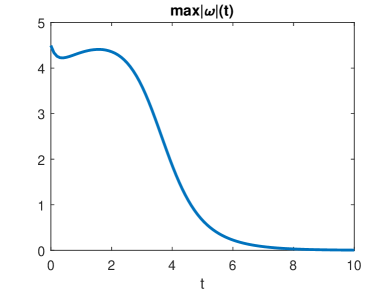
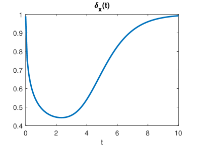
Figure 4: Evolution of $\max_{x}|\omega|(t)$ and of the distance to the closest singularity $\delta_{x}(t)$ from the real line in $x$-space for the periodic solution with parameters $a=1/2$, $\sigma=1$, $\nu=1$ and two-mode initial data (96) with $A=3.46$.

The singularity structure in $\mathbb{C}$, as determined by the AAA algorithm, consists of two double poles at $x=\pm i\delta$ and two branch cuts coming out of them vertically. There are also two more branch points at $x=\pm\pi\pm i\delta_{2}$ with $\delta_{2}>\delta$. This singularity structure, as well as the similarity exponents $\alpha$ and $\beta$, are the same as in the problem without dissipation [31]. However, the collapse takes longer to develop when there is dissipation, e.g., $t_{c}=1.15367$ compared to $t_{c}=0.491637$ in the inviscid problem when $A=4$. A more important distinction is that collapse can occur in the inviscid problem for any amplitude $A$, with the collapse time found to scale like $t_{c}\sim 1/A$.

$a$	$\sigma$	no blow up	blow up
	$2$	$A\leq 18.4$	$18.5\leq A$
	$1$	$A\leq 4.53$	$4.54\leq A$
$0$	$1/2$	$A\leq 2.35$	$2.35\leq A$
	$0$	$A\leq 1.33$	$1.34\leq A$
	$-1/2$	$A\leq 0.81$	$0.82\leq A$
	$2$	$A\leq 5.49$	$5.50\leq A$
	$1$	$A\leq 3.46$	$3.47\leq A$
$1/2$	$1/2$	$A\leq 2.64$	$2.65\leq A$
	$0$	$A\leq 1.96$	$1.97\leq A$
	$-1/2$	$A\leq 1.42$	$1.43\leq A$
	$2$	$A\leq 6.66$	$6.67\leq A$
	$1$	$A\leq 4.73$	$4.74\leq A$
$0.8$	$1/2$	$A\leq 4.01$	$4.02\leq A$
	$0$	$A\leq 3.42$	$3.43\leq A$
	$-1/2$	$A\leq 2.93$	$2.94\leq A$

Table 1: Critical amplitude $A$ for blow up starting from initial data (96) in the periodic problem with $\nu=1$. The blow up is of collapsing type (i.e., with $\alpha>0$) for $a=0,~{}1/2$, and neither collapsing nor expanding type (i.e., with $\alpha=0$) for $a=0.8$.

The dependence of the critical initial amplitude $A$ for blow up on the dissipation exponent $\sigma$, starting from initial data (96), is shown in Table 1. The critical amplitude decreases with $\sigma$, as expected, but most importantly for all values of $\sigma$ in the table we find that there is no blow up for sufficiently small data. This differs from the inviscid problem, in which blow up can occur for arbitrarily small amplitude. Of course, the absence of a blow up for $\sigma<1$ and sufficiently small data could be the consequence of restricting to the particular class of initial conditions (96). In fact, for $a=0,~{}\sigma=0,~{}\nu>0$ we have established in Section 6 that blow up occurs for arbitrarily small data of type (86) in the $L^{2}$ norm (but not in $L^{\infty}$ or $B_{0}$ norms). That data contains a pair of simple poles in the finite complex plane. Additional numerical simulations have been performed with the data (86) which (1) validates the analytical solution described in Section 6 in cases (a)-(c2) and confirms the formulas for $t_{c}$, $x_{c}$ and $\|\omega(x,t)\|_{L^{\infty}}$, $\|\omega(x,t)\|_{L^{2}}$, $\|\omega(x,t)\|_{B_{0}}$, $E_{K}(t)$; and (2) shows that blow up for this data does not occur when $\sigma\geq 1$ and the data is sufficiently small in the $L^{2},~{}L^{\infty}$ and $B_{0}$ norms. This is consistent with the analytical theory.

Examination of the solution at other values of $a$ and $\sigma\geq 1$ gives results that are consistent with Theorems 3.1 and 4.7, namely, that finite-time singularity formation in the periodic problem does not occur for sufficiently small data when using initial conditions of type (86) or (96).

7.3 Problem on the real line

In contrast to the periodic case, the problem on the real line can exhibit finite-time blow up for arbitrarily small data.

7.3.1 Schochet’s solution for $a=0$, $\sigma=2$

We have numerically computed the solution to the initial value problem (LABEL:CLM) on $x\in\mathbb{R}$ using Schochet’s initial condition. The initial singularity locations are taken on the negative imaginary axis in $\mathbb{C}$, e.g., $x_{1}(0)=-i,x_{2}(0)=-2i$, and data for $\omega=2Re(\omega_{+})$ is specified as in (42), with $A(0),B(0),C(0),D(0)$ given by (43), (44). We use the corrected values $K_{\pm}=24(3\pm\sqrt{6})$. In all cases we observe singularity motion exactly as given by (45), (46). We also observe self-similar collapse which scales precisely as predicted by (50), with collapse time given by (49). This verifies the corrected form of Schochet’s solution, and shows that it is stable to discretization and round-off errors. Crucially, this solution develops finite time singularities from arbitrarily small data.

Perturbations of Schochet’s initial data, for example by slightly altering some of the coefficients $K_{\pm}$ or $A(0)$ through $D(0)$, leads to the formation of additional branch points/cuts in the complex singularity structure. In particular, we observe the formation of a branch cut between the initial two double poles at $x_{1}(t)$ and $x_{2}(t)$ in each of $\omega_{+}$ and $\omega_{-}$ when $t>0$. Despite the change in the complex singularity structure, the solution exhibits the same self-similar blow-up as described by (50), with similarity exponents $\alpha=1$ and $\beta=2$. For small perturbations in the data, the value of $t_{c}$ is only slightly perturbed from (49).

7.3.2 Solutions for $a=1/2$, $\sigma=1$

Numerical computations of the initial value problem for $a=1/2$ and $\sigma=1$ using double pole data of the form (51) have also been performed. These give results that are in complete quantitative agreement with the analytical solution described in Section 5.2. In particular, we find that the complex singularity pattern for $t>0$ consists of two double poles as described by (51). We also find that there is blow up with the local self-similar form (60) when $\Omega(0)={\omega_{-2}}(0)/v_{c}(0)\geq 2$, and global existence with ${\omega_{-2}}(t)\rightarrow 0$ and $v_{c}(t)\rightarrow t+c$ when $\Omega(0)<2$, identical to Figure 2. This numerically validates the analysis of Section 5.2, and further shows that the analytical solution derived there is stable to discretization and round-off errors. We have additionally verified that this solution develops finite time singularities from arbitrarily small data as measured by the $L^{2}$ or $L^{\infty}$ norms of $\omega$, by taking the imaginary singularity location $v_{c}(0)$ large while retaining $\Omega(0)>2$.

Small perturbations of the initial data (51) have no effect on the complex singularity pattern of the self-similar part of the collapsing solution near $t\rightarrow t_{c}$. Blow up continues to follow the self-similar form (60) with $\alpha=1/3$ and $\beta=1$ and two double poles being the closest singularity to the real line.

7.3.3 Solutions for $a=0$, $\sigma=1$

We performed numerical computations for the initial value problem with $a=0$ and $\sigma=1$ and initial data of the form (62) containing a pair of simple poles. The computations validate (i.e., agree quantitatively) with the analytical solution (63) described in Section 5.3 by showing (1) global existence if $Re(\omega_{-1}(0))>-\nu$, (2) stationarity if $\omega_{-1}(0)=-\nu$ and (3) collapse with self-similar form (5) and $\alpha=\beta=1$ if $Re(\omega_{-1}(0))<-\nu$.

We also performed numerical computations for the initial value problem with $a=0$ and $\sigma=1$ using initial data of the form (68) which contains two pairs of simple poles. We considered the two cases $\omega_{-1,1}(0)+\omega_{-1,2}(0)\neq 0$ and $\omega_{-1,1}(0)+\omega_{-1,2}(0)=0$. The computations agree quantitatively with the analytical solutions described in Section 5.3. We are able to observe self-similar blow up in the form (5) with $\alpha=\beta=1$ and with $\alpha=\beta=2$ (see Figure 5). However, the latter type of blow up is unstable, in the sense that arbitrarily small perturbations of the initial data transform it into blow up of type (5) with $\alpha=\beta=1$ or lead to no collapse at all (see the top of Figure 5).

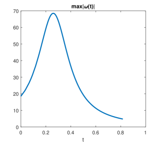
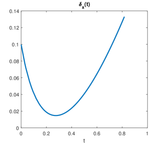
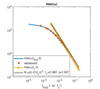
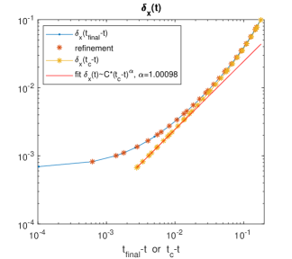
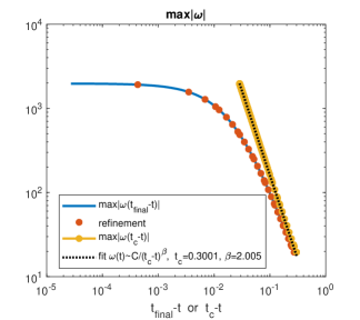
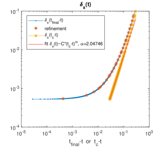
Figure 5: Evolution of $\max_{x}|\omega|(t)$ and $\delta_{x}(t)$ during numerical simulations with $a=0$, $\sigma=1$, $\nu=1$ and initial data (68), which contains two pairs of simple poles. The initial pole positions and amplitudes are $v_{c,1}(0)=0.1,v_{c,2}(0)=0.9$ and $\omega_{-1,1}(0)=-\omega_{-1,2}(0)=K$. Top: $K=-1.9$, global existence of the solution. Middle: $K=-2.1$, self-similar collapse in the form (5) with $\alpha=\beta=1$. Bottom: $K=-2$, self-similar collapse in the form (5) with $\alpha=\beta=2$. Note that in the case of collapse, data for $\mbox{max}_{x}|\omega|$ and $\delta_{x}(t)$ display linear behavior (with slope $\beta$ and $\alpha$, respectively) when plotted versus $t_{c}-t$.

Also we have found and checked numerically that the initial condition $w_{0}(x)=2\mathrm{i}A(1/(x-\mathrm{i}V_{c})^{2}-1/(x+\mathrm{i}V_{c})^{2})$ with two double poles, where $A,V_{c}>0$ are real numbers, leads to similar solutions. Each of the double poles splits into two single poles at $t=0$, one of which initially moves toward the real line while the other one moves away. This initial condition could be obtained from (68) as a limit $\epsilon\rightarrow 0$ of

$$\omega_{-1,1}(t=0)=-\omega_{-1,2}(t=0)\sim-\frac{A}{\epsilon},\quad v_{c,1}(t=0)\sim V_{c}-\epsilon,\quad v_{c,2}(t=0)\sim V_{c}+\epsilon.$$

Substitution of this initial data into the solution (74) gives

$$\omega_{-1,1}(t)=-\omega_{-1,2}(t)=-\sqrt{\frac{A}{2t}},v_{c,1}(t)=\nu t-\sqrt{2At}+V_{c},v_{c,2}(t)=\nu t+\sqrt{2At}+V_{c}.$$

If $A>2\nu V_{c}$, this solution leads to self-similar blow up in the form (5) with $\alpha=\beta=1$ at time $t_{c}=(A-\nu V_{c}-\sqrt{(A-\nu V_{c})^{2}-(\nu V_{c})^{2}})/\nu^{2}$. At the time $t=t_{c}$ the lower poles cross the real axis at $x=x_{c}=0$, so that $v_{c,1}(t_{c})=0$, with nonzero velocity $v^{\prime}_{c,1}(t_{c})<0$.

If $A=2\nu V_{c}$, this solution provides a self-similar blow up with $\alpha=\beta=2$ at the time $t_{c}=A/2=\nu V_{c}$, when the lower pole approaches the real axis at $x=x_{c}=0$ with zero velocity $v^{\prime}_{c,1}(t_{c})=0$.

For $A<2\nu V_{c}$, the solution exists for all $t>0$ since the lower pole doesn’t reach the real axis.

7.3.4 Solutions for $a=0$, $\sigma=0$

We performed numerical computations for the initial value problem with $a=0$ and $\sigma=0$ and initial data of the form (78) containing a pair of simple poles. The computations validate (i.e., agree quantitatively) with the analytical solution (79) described in Section 5.4 which exhibits global existence if $Re[\omega_{-1}(0)]>-\nu Re[v_{c}(0)]$), steady states if $Re[\omega_{-1}(0)]=-\nu Re[v_{c}(0)]$, and self-similar collapse with $\alpha=\beta=1$ if $Re[\omega_{-1}(0)]<-\nu Re[v_{c}(0)]$. We have also numerically confirmed all other formulas and claims made in Section 5.4 regarding $t_{c}$, $x_{c}$ and $\|\omega(x,t)\|_{L^{\infty}}$, $\|\omega(x,t)\|_{L^{2}}$, $\|\omega(x,t)\|_{B_{0}}$, $E_{K}(t)$.

8 Conclusion

We have shown global-in-time existence of solutions to the generalized Constantin-Lax-Majda equation with dissipation, in the case of small data in the periodic geometry, for $\sigma\geq 1$ and any $a$. This extends previous results on global existence theory from a subset of the range $a\leq-1$ to all $a$. Our analysis is by two complementary approaches. The first result, Theorem 3.1, proves that the solution exists globally in time for $\sigma\geq 1$ and sufficiently small data as measured by the Wiener norm $\|\omega\|_{B_{0}}$. Furthermore, the solution is analytic in a strip in $\mathbb{C}$ containing the real line for any $t>0$. The theorem also gives a lower bound on the critical initial magnitude of vorticity (in the Wiener norm) for global existence.

Our second main result, Theorem 4.7, shows global-in-time existence for small periodic data in $L^{2}$ when $\sigma>1$. The proof shows the solution at any time $t>0$ exists in $H^{\gamma}$ for all $1/2<\gamma<\min[1,\sigma-1/2]$. Following the approach of [19], this solution is also expected to be analytic in a strip in the complex plane for $t>0$.

The analytical theory is complemented by numerical computations for different $a$ and $\sigma$. The numerics are able to track the formation and motion of singularities in the complex plane. Computations in the periodic geometry for $\sigma\geq 1$ are always found to indicate global existence of solutions when the initial vorticity is below a critical amplitude. This is in agreement with the analytical theory. On the other hand, the numerics shows that finite-time blow up can occur for sufficiently large amplitude data. We derive a new exact analytical solution in the periodic geometry for $a=0$ and $\sigma=0$ which forms finite-time singularities for arbitrarily small $L^{2}$ data (but not for arbitrarily small data in $L^{\infty}$ or the Wiener space $B_{0}$). This result is suggestive of the existence in the periodic geometry of a critical value of $\sigma$, below which there can be singularity formation for arbitrarily small data.

In contrast, the problem on the real line can exhibit finite-time singularity formation for arbitrarily small data as measured by the $L^{2}$ or $L^{\infty}$ norm of $\omega$, at least for $\sigma=0,~{}1,$ and $2$ at various $a$. This is established by the derivation of new exact analytical solutions for $a=0$ and $1/2$. The new solutions exhibit interesting dynamics, which are further explored by numerical simulation. We also revisit an analytical solution derived by Schochet [36] for $a=0$ and $\sigma=2$, which leads to finite-time singularity formation for arbitrarily small data. A minor correction is made to the solution (after which the analytical results agree with numerical computations) and the solution is reinterpreted from the standpoint of self-similar blow up.

In future work, we will provide a comprehensive numerical investigation of finite-time singularity formation for a wide range of $a$ in both the periodic and real-line problems. Of particular interest is the effect of the dissipation on the critical parameter $a_{c}$ which separates self-similar collapsing solutions from expanding and ‘neither collapsing nor expanding’ solutions observed in the problem without dissipation [31]. Another interesting question is whether $\sigma=1$ is the optimal lower bound for which global existence for small data can be guaranteed. A related question for the problem on the real line is whether there exists a value of $\sigma$ greater than $2$ for which one can guarantee global existence for small data. These questions are left for future work.

9 Acknowledgements

D.M.A. was supported by National Science Foundation Grant DMS-1907684. M.S. was supported by National Science Foundation Grant DMS-1909407. The work of P.M.L. was supported by the National Science Foundation, Grant DMS-1814619. Simulations were performed at the Texas Advanced Computing Center using the Extreme Science and Engineering Discovery Environment (XSEDE), supported by NSF Grant ACI-1053575.

Appendix A Appendix

A.1 Proof of the inequality (12)

Given $\theta>0,$ we want to find $C\geq 0$ such that for all $(j,k)\in\mathbb{Z}^{2},$ we have

$$|k|^{\theta}\leq C(|k-j|^{\theta}+|j|^{\theta}).$$

First, note that if $k=0,$ the inequality is satisfied for any $C\geq 0.$ We now focus on the case $k\neq 0.$ Notice that if $k\neq 0$ then also $|k-j|^{\theta}+|j|^{\theta}\neq 0.$ The value $C$ may then be taken to be the maximum of

$$\frac{|k|^{\theta}}{|k-j|^{\theta}+|j|^{\theta}}=\frac{1}{\left|1-\frac{j}{k}\right|^{\theta}+\left|\frac{j}{k}\right|^{\theta}}.$$

We define $z=j/k,$ and we seek to find the maximum value for $z\in\mathbb{R}$ of the function

$$f(z)=\frac{1}{|1-z|^{\theta}+|z|^{\theta}}.$$

We consider this in three regions. First, if $z\geq 1,$ then

$$f(z)=\frac{1}{(z-1)^{\theta}+z^{\theta}}.$$

We note the values $f(1)=1$ and $\displaystyle\lim_{z\rightarrow\infty}f(z)=0.$ We compute

$$f^{\prime}(z)=-\theta\frac{(z-1)^{\theta-1}+z^{\theta-1}}{\left((z-1)^{\theta}+z^{\theta}\right)^{2}}.$$

If $f^{\prime}(z)=0,$ then $(z-1)^{\theta-1}=-z^{\theta-1},$ and this equation has no solutions on $[1,\infty).$ Therefore the maximum of $f$ for $z\in[1,\infty)$ is attained at $z=1,$ and is $f(1)=1.$

Next we consider $0\leq z\leq 1.$ On this domain, the function $f$ becomes

$$f(z)=\frac{1}{(1-z)^{\theta}+z^{\theta}}.$$

The boundary values on this domain are $f(0)=1$ and $f(1)=1.$ We take the derivative, finding

$$f^{\prime}(z)=-\theta\frac{-(1-z)^{\theta-1}+z^{\theta-1}}{\left((1-z)^{\theta}+z^{\theta}\right)^{2}}.$$

Setting $f^{\prime}(z)=0,$ we find a critical point at $z=1/2.$ At this point, we have the function value $f(1/2)=2^{\theta-1}.$ So, for $z\in[0,1],$ we have $f(z)\leq\max\{1,2^{\theta-1}\}.$

Finally, we let $z\in(-\infty,0];$ on this domain, $f$ is given by

$$f(z)=\frac{1}{(1-z)^{\theta}+(-z)^{\theta}}.$$

On this domain the boundary values are $f(0)=1$ and $\displaystyle\lim_{z\rightarrow-\infty}f(z)=0.$ The derivative of $f$ is

$$f^{\prime}(z)=-\theta\frac{-(1-z)^{\theta-1}-(-z)^{\theta-1}}{\left((1-z)^{\theta}+(-z)^{\theta}\right)^{2}}.$$

Setting $f^{\prime}(z)=0,$ we find the equation $(1-z)^{\theta-1}=-(-z)^{\theta-1}.$ There are no solutions of this, so the maximum of $f$ on the present domain is attained at $z=0,$ and is $f(0)=1.$

Overall, we have demonstrated that (12) holds with $C=\max\{1,2^{\theta-1}\}.$

A.2 Proof of Lemma 4.1

Denote the integrand in (25) as $J(t,\tau)$, and decompose the integral as

$$\int_{0}^{t}J(t,\tau)\ d\tau =\left(\int_{0}^{1}+\int_{1}^{t}\right)J(t,\tau)\ d\tau$$

$$=I_{1}+I_{2}$$

For $t\leq 2$ (say), the integral can be bounded by a constant that is independent of $t$. This follows by using $|e^{-{\hat{q}(t-\tau)}}|\leq 1$ and making the change of variable $\theta=\tau/t$ which gives

$$\int_{0}^{t}J(t,\tau)\ d\tau\leq t^{1-{\hat{\alpha}}-{\hat{\beta}}}\int_{0}^{1}\frac{1}{(1-\theta)^{\hat{\alpha}}\theta^{{\hat{\beta}}+{\hat{\delta}}}}\ d\theta,$$

which is bounded for $0\leq{\hat{\alpha}}<1$, $0\leq{\hat{\alpha}}+{\hat{\beta}}\leq 1$, $0\leq{\hat{\beta}}+{\hat{\delta}}<1$ and $0\leq t\leq 2$.

Therefore, w.l.o.g. assume $t>2$. To bound $I_{1}$, note that $e^{-{\hat{q}}(t-\tau)}\leq e^{-{\hat{q}}(t-1)}$ on the integration interval and make the change of variable $\theta=\tau/t$ to obtain

$$I_{1} \leq e^{-{\hat{q}}(t-1)}t^{1-{\hat{\alpha}}-{\hat{\beta}}}\int_{0}^{1/t}\frac{1}{(1-\theta)^{\hat{\alpha}}\theta^{{\hat{\beta}}+{\hat{\delta}}}}\ d\theta$$

$$\leq 2^{\hat{\alpha}}e^{-{\hat{q}}(t-1)}t^{1-{\hat{\alpha}}-{\hat{\beta}}}\int_{0}^{1/t}\frac{1}{\theta^{{\hat{\beta}}+{\hat{\delta}}}}\ d\theta$$

$$\leq\frac{2^{\hat{\alpha}}}{1-{\hat{\beta}}-{\hat{\delta}}}e^{-{\hat{q}}(t-1)}t^{{\hat{\delta}}-{\hat{\alpha}}},$$

where we have used $1/(1-\theta)^{\hat{\alpha}}\leq 2^{\hat{\alpha}}$ on $\theta\in[0,1/t]$ when $t\geq 2$. Hence $I_{1}<C$ for $t>2$. To bound $I_{2}$, note that in the integration interval $\tau^{\hat{\beta}}>1$ and make the change of variable $v=t-\tau$ to obtain

$$I_{2} \leq\int_{0}^{t-1}\frac{e^{-{\hat{q}}v}}{v^{\hat{\alpha}}}\frac{1}{(1-\frac{v}{t})^{\hat{\delta}}}\ d\tau$$

$$=\left(\int_{0}^{(t-1)/2}+\int_{(t-1)/2}^{t-1}\right)\frac{e^{-{\hat{q}}v}}{v^{\hat{\alpha}}}\frac{1}{(1-\frac{v}{t})^{\hat{\delta}}}\ dv$$

$$=J_{1}+J_{2}.$$

$J_{1}$ is bounded as

$$J_{1} \leq\left(\frac{1}{2}+\frac{1}{2t}\right)^{-{\hat{\delta}}}\int_{0}^{\infty}\frac{e^{-{\hat{q}}v}}{v^{\hat{\alpha}}}\ dv$$

$$\leq C,$$

while $J_{2}$ satisfies the estimate

$$J_{2} \leq\left(\frac{t-1}{2}\right)^{-{\hat{\alpha}}}e^{-{\hat{q}}\left(\frac{t-1}{2}\right)}\int_{(t-1)/2}^{t-1}\frac{dv}{(1-\frac{v}{t})^{\hat{\delta}}}$$

$$\leq 2^{\hat{\alpha}}e^{-{\hat{q}}\left(\frac{t-1}{2}\right)}\frac{t}{1-{\hat{\delta}}}$$

$$\leq C.$$

Hence $I_{2}<C$ for $t>2$, and the result follows.

A.3 Proof of Lemma 4.3

Let $H_{t}(k)=e^{-2t|k|^{\sigma}}$, and assume $\sigma>0$. Then

$$\sum_{k\in\mathbb{Z}}H_{t}(k) =1+2\sum_{k=1}^{\infty}H_{t}(k)$$

$$\leq 1+2\left(H_{t}(1)+\int_{1}^{\infty}H_{t}(k)\ dk\right).$$ (97)

Substitute $u=2tk^{\sigma}$ into the integral in (97) and estimate it as

$$\int_{1}^{\infty}H_{t}(k)\ dk =\frac{(2t)^{-1/\sigma}}{\sigma}\int_{2t}^{\infty}e^{-u}u^{1/\sigma-1}\ du$$

$$\leq Ct^{-1/\sigma}e^{-t}.$$ (98)

The second inequality follows from elementary estimates.

Substitute (98) and $H_{t}(1)=e^{-2t}$ into (97) to obtain

$$\sum_{k\in\mathbb{Z}}e^{-2t|k|^{\sigma}}\leq 1+2\left(e^{-2t}+Ce^{-t}t^{-1/\sigma}\right)$$ (99)

which can be easily simplified to obtain the final form (32). Finally, note that if the $k=0$ term in the norm $\|e^{-t\rho(\cdot)}\|_{l_{2}}$ is omitted, which in turn implies that the first $1$ in (97), (99), and (32) can be omitted.

References

- [1] D.M. Ambrose. The radius of analyticity for solutions to a problem in epitaxial growth on the torus. Bull. London Math. Soc., 51(5):877–886, 2019.
- [2] D.M. Ambrose and A.L. Mazzucato. Global existence and analyticity for the 2D Kuramoto-Sivashinsky equation. J. Dynam. Differential Equations, 31(3):1525–1547, 2019.
- [3] G. Baker, R.E. Caflisch, and M. Siegel. Singularity formation during Rayleigh–Taylor instability. Journal of Fluid Mechanics, 252:51–78, 1993.
- [4] Michael P. Brenner, Peter Constantin, Leo P. Kadanoff, Alain Schenkel, and Shankar C. Venkataramani. Diffusion, attraction and collapse. Nonlinearity, 12(4):1071–1098, 1999.
- [5] F. Calogero. Classical Many-Body Problems Amenable to Exact Treatments. Springer-Verlag, Berlin, 2001.
- [6] G.F. Carrier, M. Krook, and C.E. Pearson. Functions of a Complex Variable. McGraw-Hill, New York, 1966.
- [7] A. Castro and D. Córdoba. Infinite energy solutions of the surface quasi-geostrophic equation. Adv. Math., 225(4):1820–1829, 2010.
- [8] J. Chen. Singularity formation and global well-posedness for the generalized Constantin–Lax–Majda equation with dissipation. Nonlinearity, 33(5):2502, 2020.
- [9] J. Chen, T.Y. Hou, and D. Huang. On the finite time blowup of the De Gregorio model for the 3D Euler equations. Commun. Pure Appl. Math., 74(6):1282–1350, 2021.
- [10] S. Childress and Percus J.K. Nonlinear aspect of chemotaxis. Math. Bio., 56:217–237, 1981.
- [11] P. Constantin, P. D. Lax, and A. Majda. A simple one-dimensional model for the three-dimensional vorticity equation. Commun. Pure Appl. Math., 38(6):715–724, 1985.
- [12] G.J. Cooper and J.H. Verner. Some Explicit Runge-Kutta Methods of High Order. SIAM Journal on Numerical Analysis, 9(3):389–405, 1972.
- [13] A. Córdoba, D. Córdoba, and M.A. Fontelos. Formation of singularities for a transport equation with nonlocal velocity. Ann. Math., pages 1377–1389, 2005.
- [14] H. Dong. Well-posedness for a transport equation with nonlocal velocity. J. Funct. Anal., 255(11):3070–3097, 2008.
- [15] J. Duchon and R. Robert. Global vortex sheet solutions of Euler equations in the plane. J. Differ. Equ., 73(2):215–224, 1988.
- [16] Sergey A. Dyachenko, Pavel M. Lushnikov, and Natalia Vladimirova. Logarithmic scaling of the collapse in the critical Keller-Segel equation. Nonlinearity, 26:3011–3041, 2013.
- [17] T.M. Elgindi and I.-J. Jeong. On the effects of advection and vortex stretching. Archive for Rational Mechanics and Analysis, 235:1763–1817, 2020.
- [18] G.B. Folland. Introduction to partial differential equations. Princeton University Press, 2020.
- [19] Z. Grujić and I. Kukavica. A remark on time-analyticity for the Kuramoto–Sivashinsky equation. Nonlinear Anal. Theory Methods, 52(1):69–78, 2003.
- [20] T.Y. Hou, T. Jin, and P. Liu. Potential singularity for a family of models of the axisymmetric incompressible flow. J. Nonlinear Sci., 28(6):2217–2247, 2018.
- [21] T.Y. Hou, Z. Lei, G. Luo, S. Wang, and C. Zou. On finite time singularity and global regularity of an axisymmetric model for the 3D Euler equations. Archive for Rational Mechanics and Analysis, 212(2):683–706, 2014.
- [22] T.Y Hou, Z. Shi, and S. Wang. On singularity formation of a 3D model for incompressible Navier-Stokes equations. Adv. Math., 230(2):607–641, 2012.
- [23] H. Jia, S. Stewart, and V. Sverak. On the De Gregorio modification of the Constantin–Lax–Majda model. Arch. Ration. Mech. and Anal., 231(2):1269–1304, 2019.
- [24] A. Kiselev. Regularity and blow up for active scalars. Math. Model. Nat. Phenom., 5(4):225–255, 2010.
- [25] E. A. Kuznetsov and V. E. Zakharov. Wave Collapse. World Scientific Publishing Company, New York, 2007.
- [26] Z. Lei, J. Liu, and X. Ren. On the Constantin–Lax–Majda Model with convection. Commun. Math. Phys., pages 1–19, 2019.
- [27] D. Li and J. Rodrigo. Blow-up of solutions for a 1D transport equation with nonlocal velocity and supercritical dissipation. Adv. Math., 217(6):2563–2568, 2008.
- [28] P. M. Lushnikov. Exactly integrable dynamics of interface between ideal fluid and light viscous fluid. Physics Letters A, 329:49 – 54, 2004.
- [29] P. M. Lushnikov and N. M. Zubarev. Exact solutions for nonlinear development of a Kelvin-Helmholtz instability for the counterflow of superfluid and normal components of Helium II. Phys. Rev. Lett., 120:204504, 2018.
- [30] Pavel M. Lushnikov, Sergey A. Dyachenko, and Natalia Vladimirova. Beyond leading-order logarithmic scaling in the catastrophic self-focusing of a laser beam in Kerr media. Phys. Rev. A, 88:013845, 2013.
- [31] P.M. Lushnikov, D.A. Silantyev, and M. Siegel. Collapse versus blow-up and global existence in the generalized Constantin–Lax–Majda equation. J. Nonlinear Sci., 31(5):1–56, 2021.
- [32] Y. Nakatsukasa, O. Sète, and L.N. Trefethen. The AAA algorithm for rational approximation. SIAM J. Sci. Comp., 40(3):A1494–A1522, 2018.
- [33] H. Okamoto and K. Ohkitani. On the role of the convection term in the equations of motion of incompressible fluid. J. Phys. Soc. Japan, 74(10):2737–2742, 2005.
- [34] H. Okamoto, T. Sakajo, and M. Wunsch. On a generalization of the Constantin–Lax–Majda equation. Nonlinearity, 21(10):2447, 2008.
- [35] D.A. Pugh. Development of vortex sheets in Boussinesq flows – formation of singularities. PhD Thesis, Imperial College, 1989.
- [36] S. Schochet. Explicit solutions of the viscous model vorticity equation. Comm. Pure Appl. Math., 39(4):531–537, 1986.
- [37] D. Senouf, R. Caflisch, and N. Ercolani. Pole dynamics and oscillations for the complex Burgers equation in the small-dispersion limit. Nonlinearity, 9:1671, 1996.
- [38] D. A. Silantyev, P. M. Lushnikov, and H. A. Rose. Langmuir wave filamentation in the kinetic regime. I. Filamentation instability of Bernstein-Greene-Kruskal modes in multidimensional Vlasov simulations. Phys. of Plasmas, 24:042104, 2017.
- [39] L. Silvestre and V. Vicol. On a transport equation with nonlocal drift. Trans. Am. Math. Soc., 368(9):6159–6188, 2016.
- [40] C. Sulem and P. L. Sulem. Nonlinear Schrödinger Equations: Self-Focusing and Wave Collapse. World Scientific, New York, 1999.
- [41] C. Sulem, P.-L. Sulem, and H. Frisch. Tracing complex singularities with spectral methods. J. Comput. Phys., 50:138–161, 1983.
- [42] M. Wunsch. The generalized Constantin-Lax-Majda equation revisited. Commun. Math. Sci., 9(3):929–936, 2011.
- [43] V. E. Zakharov. Collapse of langmuir waves. Sov. Phys. JETP, 35:908, 1972.