3DVerifier: Efficient Robustness Verification for 3D Point Cloud Models

Abstract

3D point cloud models are widely applied in safety-critical scenes, which delivers an urgent need to obtain more solid proofs to verify the robustness of models. Existing verification method for point cloud model is time-expensive and computationally unattainable on large networks. Additionally, they cannot handle the complete PointNet model with joint alignment network (JANet) that contains multiplication layers, which effectively boosts the performance of 3D models. This motivates us to design a more efficient and general framework to verify various architectures of point cloud models. The key challenges in verifying the large-scale complete PointNet models are addressed as dealing with the cross-non-linearity operations in the multiplication layers and the high computational complexity of high-dimensional point cloud inputs and added layers. Thus, we propose an efficient verification framework, 3DVerifier, to tackle both challenges by adopting a linear relaxation function to bound the multiplication layer and combining forward and backward propagation to compute the certified bounds of the outputs of the point cloud models. Our comprehensive experiments demonstrate that 3DVerifier outperforms existing verification algorithms for 3D models in terms of both efficiency and accuracy. Notably, our approach achieves an orders-of-magnitude improvement in verification efficiency for the large network, and the obtained certified bounds are also significantly tighter than the state-of-the-art verifiers. We release our tool 3DVerifier via https://github.com/TrustAI/3DVerifier for use by the community.

1 Introduction

Recent years have witnessed increasing interest in 3D object detection, and Deep Neural Networks (DNNs) have also demonstrated their remarkable performance in this area (Qi et al, 2017a, b). For 3D object detectors, the point clouds are utilized to represent 3D objects, which are usually the raw data gained from LIDARs and depth cameras. Such 3D deep learning models have been widely employed in multiple safety-critical applications such as motion planning  (Varley et al, 2017), virtual reality  (Stets et al, 2017), and autonomous driving  (Chen et al, 2017; Liang et al, 2018). However, extensive research has shown that DNNs are vulnerable to adversarial attacks, appearing as adding a small amount of non-random, ideally human-invisible, perturbations on the input will cause DNNs to make abominable predictions  (Szegedy et al, 2014; Carlini and Wagner, 2017; Jin et al, 2020). Therefore, there is an urgent need to address such safety concerns on DNNs caused by adversarial examples, especially on safety-critical 3D object detection scenarios.

Recently, most works on analyzing the robustness of 3D models mainly focus on adversarial attacks with an aim to reveal the model’s vulnerabilities under different types of perturbations, such as adding or removing points, and shifting positions of points  (Liu et al, 2019; Zhang et al, 2019a). In the meanwhile, adversarial defenses are also proposed to detect or prevent these adversarial attacks  (Zhang et al, 2019a; Zhou et al, 2019). However, as Tramer et al (2020) and Athalye et al (2018) indicated, even though these defenses are effective for some attacks, they still can be broken by other stronger attacks. Thereby, we need a more solid solution, ideally with provable guarantees, to verify whether the model is robust to any adversarial attacks within an allowed perturbation budget. This technique is also generally regarded as verification on (local) adversarial robustness in the community. So far, various solutions have been proposed to tackle robustness verification, but they mostly focus on the image domain  (Boopathy et al, 2019; Singh et al, 2019; Tjeng et al, 2018; Jin et al, 2022). Verifying the adversarial robustness of 3D point cloud models, by contrast, is barely explored by the community. As far as we know, 3DCertify, proposed by Lorenz et al (2021) is the first and also the only work to verify the robustness of 3D models. Although 3DCertify is very inspiring, it has yet completely resolved some key challenges on robustness verification for 3D models according to our empirical study.

Firstly, as the first verification tool for 3D models, 3DCertify is time-consuming and thus not computationally attainable on large neural networks. As 3DCertify is built upon DeepPoly  (Singh et al, 2019), when directly applying the relaxation algorithm that is specifically designed for images on the high-dimensional point clouds, it will result in out-of-memory issues and cause the termination of the verification. Moreover, 3DCertify can only verify a simplified PointNet model without Joint Alignment Network (JANet) consisting of matrix multiplication operations. Figure 1 illustrates the abstract architecture of a complete PointNet  (Qi et al, 2017a), one of the most widely used models on 3D object detection. As we can see, since the learnt representations are expected to be invariant to spatial transformations, JANet is the key enabler in PointNet to achieve this geometric invariant functionality by adopting the T-Net and matrix multiplications. Recent research also demonstrates that JANet is an essential for boosting the performance of PointNet  (Qi et al, 2017a) and thus widely applied in some safety-critical tasks  (Paigwar et al, 2019; Aoki et al, 2019; Chen et al, 2021). Thirdly, 3DCertify can only work on $l_{\infty}$-norm metric, however, arguably, some researchers in the community regard other $l_{p}$-norm metrics such as $l_{1}$, $l_{2}$-norm metrics are equally (if not more) important in the study of adversarial robustness  (Boopathy et al, 2019; Weng et al, 2018). Thus, a robustness verification tool that can work on a wide range of $l_{p}$-norm metrics is also worthy of a comprehensive exploration.

Figure 1: The abstract framework of the PonitNet with joint alignment network (JANet), where MLP stands for multi-layer perceptron.

Thus, motivated by the aforementioned challenges yet to be resolved, this paper aims to design an efficient and scalable robustness verification tool that can handle a wide range of 3D models, including those with JANet structures under multiple $l_{p}$-norm metrics including $l_{\infty}$, $l_{1}$, and $l_{2}$-norm. We achieve the verification efficiently by adapting the efficient layer-by-layer certification framework used in  (Weng et al, 2018; Boopathy et al, 2019). Considering that these verifiers are designed for images and cannot be applied in larger-scale 3D point cloud models, we introduce a novel relaxation function of global max pooling to make it applicable and efficient on PointNet. Moreover, the multiplication layers in the JANet structure involves two variables under perturbations, which brings the cross-non-linearity. Due to the high dimensionality in 3D models, such cross-non-linearity results in significant computational overhead for computing a tight bound. Inspired by the recent advance of certification on transformers  (Shi et al, 2020), we propose closed-form linear functions to bound the multiplication layer and combine forward and backward propagation to speed up the bound computation, which can be calculated in only $O(1)$ complexity. In summary, the main contributions of this paper are listed as below.

• Our method can achieve an efficient verification. We design a relaxation algorithm to resolve the cross-non-linearity challenge by combining the forward and backwards propagation, enabling an efficient yet tight verification on matrix multiplications.

• We design an efficient and scalable verification tool, 3DVerifier, with provable guarantees. It is a general framework that can verify the robustness for a wide range of 3D model architectures, especially it can work on complete and large-scale 3D models under $l_{\infty}$, $l_{1}$, and $l_{2}$-norm perturbations.

• 3DVerifier, as far as we know, is one of the very few works on 3D model verification, which is more advanced than the existing work, 3DCertify, in terms of efficiency, scalability and tightness of the certified bounds.

2 Related Work

3D Deep Learning Models: As the raw data of point clouds comes directly from real-world sensors, such as LIDARs and depth cameras, point clouds are widely used to represent 3D objects for the deep learning classification task. To deal with the unordered point clouds, Qi et al (2017a) proposed the PointNet model, which utilised the global max-pooling layer to assemble features of points and the joint alignment network (JANet). Then, Qi et al (2017b) extended the PointNet by using the spacial neighbor graphs.

Adversarial Attacks on 3D Point Clouds Classification: Szegedy et al (2014) first proposed the concepts of adversarial attacks and indicated that the neural networks are vulnerable to the well-crafted imperceptible perturbation. Xiang et al (2019) claimed that they are the first work to perform extensive adversarial attacks on 3D point cloud models by perturbing the positions of points or generating new points. Recent works extended the adversarial attacks for images to 3D point clouds by perturbing points and generating new points  (Goodfellow et al, 2014; Zhang et al, 2019a; Lee et al, 2020). Additionally, Cao et al (2019) proposed the adversarial attacks on LiDAR systems.Wicker and Kwiatkowska (2019) used occlusion attack and Zhao et al (2020) proposed isometric transformations attack. Towards these adversarial attacks, corresponding defense techniques are developed  (Zhang et al, 2019a; Zhou et al, 2019), which are more effective than adversarial training such as  (Liu et al, 2019; Zhang et al, 2019b). However, Sun et al (2020) examined existing defense works and pointed out that those defenses are still vulnerable to more powerful attacks. Thus, Lorenz et al (2021) proposed the first verification algorithm for 3D point cloud models with provable robustness bounds.

Verification on Neural Networks: The robustness verification aims to find a guaranteed region that any input in this region leads to the same predicted label. For image classification, the region is bounded by a $l_{p}$-norm ball with a radius of $\epsilon$, and the aim is to maximize the $\epsilon$. For point clouds models, we reformulate the goal to find the maximum $\epsilon$ that any distortion applied on the position of the point within the region cannot alter the predicted label. Numerous works have attempted to find the exact value in the image domain $\epsilon$  (Katz et al, 2017; Tjeng et al, 2018; Bunel et al, 2017). Yet these approaches are designed for small networks. Some works focus on computing a certified lower bound for the $\epsilon$. To handle the non-linearity operations in the neural network, the convex relaxation is proposed to approximate the bounds for the ReLU layer  (Salman et al, 2019). Wong and Kolter (2018) and Dvijotham et al (2018) introduced a dual approach to form the relaxation. Several studies computed the bounds via linear-by-linear approximation  (Wang et al, 2018; Weng et al, 2018; Zhang et al, 2018) or abstract domain interpretation  (Gehr et al, 2018; Singh et al, 2019).

While for the 3D point cloud models, only Lorenz et al (2021) proposed the 3Dcertify. However, their method is time expensive and can not handle the JANet in the full PointNet models. Thus, in this paper, we build a more efficient and general verification framework to obtain the certified bounds.

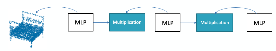
Figure 2: Illustration of the combining forward and backward propagation process. The architecture in the MLP block contains convolution with ReLU activation function, batch normalization and pooling. Inside the MLP block, the bounds are computed by backward propagation.

3 Methodology: 3DVerifier

3.1 Overview

The clean input point cloud $\mathbf{P}_{0}$ with $n$ points can be defined as $\mathbf{P}_{0}=\{\mathbf{p_{0}}^{(i)}\mid\mathbf{p_{0}}^{(i)}\in\mathbb{R}^{3},i=1,...,n\}$, where each point $\mathbf{p_{0}}^{(i)}$ is represented in a 3D space coordinate $(x,y,z)$. We choose the points that are correctly recognized by the classifier $C$ as inputs to verify the robustness of $C$.

Throughout this paper, we will perturb the points by shifting their positions in the 3D space within a distance bounded by the $l_{p}$-norm ball. Given the perturbed input $\mathbf{P}=\{\mathbf{p}^{(i)}\mid\mathbf{p}^{(i)}\in\mathbb{R}^{3},i=1,...,n\}$ that is in the $l_{p}$-norm ball $\mathbb{S}_{p}\left(\mathbf{p}_{0}^{(i)},\epsilon\right):=\left\{\mathbf{p}^{(i)}\mid\left\|\mathbf{p}^{(i)}-\mathbf{p}_{0}^{(i)}\right\|_{p}\leq\epsilon,i=1,...,n\right\}$, we aim to verify whether the predicted label of the model is stable within the region $\mathbb{S}_{p}$. This can be solved by finding the minimum adversarial perturbation $\epsilon_{min}$ via binary search, such that $\exists\mathbf{P}\in\mathbb{S}_{p}\left(\mathbf{P}_{0},\epsilon_{min}\right)$, argmax $C(\mathbf{P})\neq c$, where $c=$argmax $C(\mathbf{P_{0}})$. Such $\epsilon_{min}$ is also referred as the untargeted robustness. As for the targeted robustness, it can be interpreted as that the prediction output score for the true class is always greater than that for the target class.

Assuming that the target class is $t$, the objective function is:

$$\min\left\{y_{c}(\mathbf{P})-y_{t}(\mathbf{P})\right\}:=\sigma_{\epsilon},\qquad s.t\quad\|\mathbf{p}^{{k}}-\mathbf{p}_{0}^{{k}}\|_{p}\leq\epsilon,(k=1,2,...,n),$$ (1)

where $y_{c}$ represents the logit output for class $c$ and $y_{t}$ is for the target class $t$. $\mathbf{P}$ is the set of points that is centred around the original points set $\mathbf{P}_{0}$ within the $l_{p}$-norm ball with radius $\epsilon$. Thus, if $\sigma_{\epsilon}>0$, the logit output of the true class $c$ is always greater than the target class, which means that the predicted label cannot be $t$. Due to the fact that finding the exact output of $\sigma_{\epsilon}$ is an NP-hard problem (Katz et al, 2017), the objective function of our work can be alternatively altered as computing the lower bound of $\sigma_{\epsilon}$. By applying binary search to update the perturbation $\epsilon$, we can find the minimum adversarial perturbation. Equivalently, the maximum $\epsilon_{cert}$ that does not alter the predicted label can be attained. Thus, in this paper, we aim to compute the certified lower bound of $\sigma_{\epsilon_{cert}}$.

3.2 Generic Framework

To obtain the lower bound of $\sigma_{\epsilon}$ for the $l_{p}$-norm ball bounded model, we propagate the bound of each neuron layer by layer. As mentioned previously, most structures employed by the 3D point cloud models are similar to the traditional image classifiers, such as the convolution layer, batch normalization layer, and pooling layer. The most distinctive structure of the point clouds classifier, like the PointNet  (Qi et al, 2017a), is the JANet structure. Thus, to compute the logit outputs of the neural network, our verification algorithm adopt three types of formulas to handle different operations: 1) linear operations (e.g. convolution, batch normalization and average pooling), 2) non-linear operation (e.g. ReLU activation function and max pooling), 3) multiplication operation.

Let $\Phi^{l}(\mathbf{P})$ be the output of neurons in the layer $l$ with point clouds input $\mathbf{P}$. The input layer can be represented as $\Phi^{0}(\mathbf{P})=\mathbf{P}$. Suppose that the total number of layers in the classifier is $m$, $\Phi^{m}(\mathbf{P})$ is defined as the output of the neural network. In order to verify the classifier, we aim to derive a linear function to obtain the global upper bound $u$ and lower bound $l$ for each layer output $\Phi^{l}(\mathbf{P})$ for $\mathbf{P}\in\mathbb{S}_{p}\left(\mathbf{P}_{0},\epsilon\right)$.

The bounds are derived layer by layer from the first layer to the final layer. We have full access to all parameters of the classifier, such as weights $\mathbf{W}$ and bias $\mathbf{b}$. To calculate the output for each neuron, we show below the linear functions to obtain the bounds of the $l$-th layer for the neuron in position $(x,y)$ based on the previous $l^{\prime}$-th layer:

$$\sum\limits_{i,j}\mathbf{A}_{(x,y,i,j)}^{\left(l,l^{\prime}\right),L}\Phi_{(x+i,j)}^{l^{\prime}}(\mathbf{P})+\mathbf{B}_{(x,y)}^{\left(l,l^{\prime}\right),L}\leq\Phi_{(x,y)}^{l}(\mathbf{P})\leq\sum\limits_{i,j}\mathbf{A}_{(x,y,i,j)}^{\left(l,l^{\prime}\right),U}\Phi_{(x+i,j)}^{l^{\prime}}(\mathbf{P})+\mathbf{B}_{(x,y)}^{\left(l,l^{\prime}\right),U},$$ (2)

where $\mathbf{A}^{L},\mathbf{B}^{L},\mathbf{A}^{U},\mathbf{B}^{U}$ are weight and bias matrix parameters of the linear function for lower and upper bound calculations respectively. $\mathbf{A}$ and $\mathbf{B}$ are initially assigned as identity matrix ($\mathbf{I}$) and zeros matrix ($\mathbf{0}$), respectively, to keep the same output of $\Phi_{(x,y)}^{l}$ when $l=l^{\prime}$. To calculate the bounds of current layer, we take backward propagation to previous layers. The $\Phi_{(x+i,j)}^{l^{\prime}}$ is substituted by the linear function of the previous layer recursively until it reaches the first layer ($l^{\prime}=0$). After that, the output of each layer can be formed by a linear function of the first layer ($\Phi^{0}(\mathbf{P})=\mathbf{P}$), as:

$$\mathbf{A}^{(l,0),L}*\mathbf{P}+\mathbf{B}^{(l,0),L}\leq\Phi^{l}(\mathbf{P})\leq\mathbf{A}^{(l,0),U}*\mathbf{P}+\mathbf{B}^{(l,0),U}.$$ (3)

Since the perturbation added to the point clouds input is bounded by the $l_{p}$-norm ball, $\mathbf{p}\in\mathbb{S}_{p}\left(\mathbf{p}_{0},\epsilon\right)$, to compute the global bounds we need to minimize the lower bound and maximize the upper bound in Eq. 3 over the input region. Thereby, the linear function to compute the global bounds for the $l$-th layer can be represented as:

$$\Phi_{x,y}^{l,U/L}=\pm\epsilon\|\mathbf{A}_{(x,y,:,:)}^{\left(l,0\right),U/L}\|_{q}+\sum\limits_{i,j}\mathbf{A}_{(x,y,i,j)}^{\left(l,0\right),U/L}\mathbf{p}_{0}^{(x+i,j)}+\mathbf{B}_{(x,y)}^{\left(l,0\right),U/L},$$ (4)

where $\|\mathbf{A}\|_{q}$ is the $l_{q}$-norm of $\mathbf{A}$ and $1/p+1/q=1$ with $p,q>1$, “U/L” denotes that the equations are formulated for the upper bounds and lower bounds, respectively. This generic framework resembles to CROWN  (Zhang et al, 2018), which is widely utilised in the verification works to verify feed-forward neural networks (e.g. CNN-Cert  (Boopathy et al, 2019), Transformer Verification  (Shi et al, 2020)). Unlike existing frameworks based on CROWN, we further extend the algorithm to verify point clouds classifiers.

3.3 Functions for linear and non-linear operation

As the linear and nonlinear functions are basic operations in the neural network, we first adapt the framework given in  (Boopathy et al, 2019) to 3D point cloud models. In section 3.4, we will present our novel technique for JANet.

Functions for linear operation. Suppose the output of the $l^{\prime}$-th layer, $\Phi^{l^{\prime}}(\mathbf{P})$, can be computed by the output of the ($l^{\prime}$-1)-th layer, $\Phi^{l^{\prime}-1}(\mathbf{P})$, by the linear function $\Phi^{l^{\prime}}(\mathbf{P})=\mathbf{W}^{l^{\prime}}*\Phi^{l^{\prime}-1}(\mathbf{P})+\mathbf{b}^{l^{\prime}}$, where $\mathbf{W}^{l^{\prime}}$ and $\mathbf{b}^{l^{\prime}}$ are parameters of the function in the layer $l^{\prime}$. Thus the Eq. 2 can be propagated from the layer $l$ to the layer $l^{\prime}-1$ by substituting $\Phi^{l^{\prime}}(\mathbf{P})$.

$$\begin{array}[]{l}\Phi_{(x,y)}^{l,U/L}(\mathbf{P})=\sum\limits_{i,j}\mathbf{A}_{(x,y,i,j)}^{\left(l,l^{\prime}\right),U/L}\Phi_{(x+i,j)}^{l^{\prime}}(\mathbf{P})+\mathbf{B}_{(x,y)}^{\left(l,l^{\prime}\right),U/L}\\ =\sum\limits_{i,j}\mathbf{A}_{(x,y,i,j)}^{\left(l,l^{\prime}\right),U/L}(\sum\limits_{k}\mathbf{W}^{l^{\prime}}_{(k,j)}\Phi^{l^{\prime}-1}_{(x+i,k)}(\mathbf{P})+\mathbf{b}^{l^{\prime}}_{x+i,j})+\mathbf{B}_{(x,y)}^{\left(l,l^{\prime}\right),U/L}\\ =\sum\limits_{i,k}\mathbf{A}_{(x,y,i,k)}^{\left(l,l^{\prime}-1\right),U/L}\Phi^{l^{\prime}-1}_{(x+i,k)}(\mathbf{P})+\mathbf{B}_{(x,y)}^{\left(l,l^{\prime}-1\right),U/L}\end{array}$$

Functions for basic non-linear operation. For the $l^{\prime}$-th layer with non-linear operations, we apply two linear functions to bound $\Phi^{\left(l^{\prime}\right)}(\mathbf{P})$:

$$\alpha^{l^{\prime},L}\Phi^{l^{\prime}-1}(\mathbf{P})+\beta^{l^{\prime},L}\leq\Phi^{\left(l^{\prime}\right)}(\mathbf{P})\leq\alpha^{l^{\prime},U}\Phi^{l^{\prime}-1}(\mathbf{P})+\beta^{l^{\prime},U}.$$

Given the bounds of $\Phi^{\left(l^{\prime}-1\right)}(\mathbf{P})$, the corresponding parameter $\alpha^{L},\alpha^{U},\beta^{L},\beta^{U}$ can be chosen appropriately. The functions to obtain the parameters are presented in Appendix A.

After computing the corresponding $\alpha^{L},\alpha^{U},\beta^{L},\beta^{U}$, we back propagate the Eq.2 to the ($l^{\prime}$-1)-th layer:

$$\begin{array}[]{l}\Phi_{(x,y)}^{l,U/L}(\mathbf{P})=\sum\limits_{i,j}\mathbf{A}_{(x,y,i,j)}^{\left(l,l^{\prime}\right),U/L}\Phi_{(x+i,j)}^{l^{\prime}}(\mathbf{P})+\mathbf{B}_{(x,y)}^{\left(l,l^{\prime}\right),U/L}\\ =\sum\limits_{i,j}\mathbf{A}_{(x,y,i,j)}^{\left(l,l^{\prime}\right),U/L,+}*(\alpha^{l^{\prime},U/L}_{(x+i,j)}\Phi^{l^{\prime}-1}(\mathbf{P})_{(x+i,j)}+\beta_{(x+i,j)}^{l^{\prime},U/L})\\ +\sum\limits_{i,j}\mathbf{A}_{(x,y,i,j)}^{\left(l,l^{\prime}\right),U/L,-}*(\alpha^{l^{\prime},L/U}_{(x+i,j)}\Phi^{l^{\prime}-1}(\mathbf{P})_{(x+i,j)}+\beta_{(x+i,j)}^{l^{\prime},L/U})\\ =\sum\limits_{i,j}\mathbf{A}_{(x,y,i,j)}^{\left(l,l^{\prime}-1\right),U/L}\Phi_{(x+i,j)}^{l^{\prime}}(\mathbf{P})+\mathbf{B}_{(x,y)}^{\left(l,l^{\prime}-1\right),U/L},\end{array}$$

where if $\mathbf{A}_{(x,y,i,j)}^{\left(l,l^{\prime}\right),U/L}$ is a positive element of $\mathbf{A}_{(:,:,:,j)}^{\left(l,l^{\prime}\right),U/L}$, then $\mathbf{A}_{(x,y,i,j)}^{\left(l,l^{\prime}\right),U/L,+}=\mathbf{A}_{(x,y,i,j)}^{\left(l,l^{\prime}\right),U/L}$ and $\mathbf{A}_{(x,y,i,j)}^{\left(l,l^{\prime}\right),U/L,-}=0$; otherwise, $\mathbf{A}_{(x,y,i,j)}^{\left(l,l^{\prime}\right),U/L,-}=\mathbf{A}_{(x,y,i,j)}^{\left(l,l^{\prime}\right),U/L}$ and $\mathbf{A}_{(x,y,i,j)}^{\left(l,l^{\prime}\right),U/L,+}=0$.

3.4 Functions for Multiplication Layer

The most critical structure in the PointNet model is the JANet, which contains the multiplication layers. For the multiplication, assume that it takes the output of previous layer ($\Phi^{l^{\prime}-1}(\mathbf{P})$) and ($l^{\prime}$-$r$)-th layer ($\Phi^{l^{\prime}-r}(\mathbf{P})$, r $\in[1,l^{\prime}]$) as inputs, the output of $\Phi^{l^{\prime}}(\mathbf{P})$ can be calculated by: $\Phi_{(x,y)}^{l^{\prime}}(\mathbf{P})=\sum\limits_{k=1}^{d_{k}}\Phi_{(x,k)}^{l^{\prime}-r}(\mathbf{P})*\Phi^{l^{\prime}-1}_{(k,y)}(\mathbf{P})$, where $d_{k}$ is the dimension of $\Phi_{(x,:)}^{l^{\prime}-r}(\mathbf{P})$ and $\Phi^{l^{\prime}-1}_{(:,y)}(\mathbf{P})$. As the Transformer contains multiplication operation in self-attention layers, inspired by the Transformer verifier  (Shi et al, 2020), we proposed our algorithm for point clouds models.

In the JANet, before the multiplication layer, there is one reshape layer and one pooling layer. To simplify the computation, we choose the $\Phi^{l^{\prime}-1}$ as the output of pooling layer, by using $h=d_{k}*(k-1)+y$ to represent the transformation in the reshape layer. The equation to compute $\Phi^{l^{\prime}-1}(\mathbf{P})$ can be rewritten as: $\Phi_{(x,y)}^{l^{\prime}}(\mathbf{P})=\sum\limits_{k=1}^{d_{k}}\Phi_{(x,k)}^{l^{\prime}-r}(\mathbf{P})*\Phi^{l^{\prime}-1}_{(0,h)}(\mathbf{P}),$ where $h=d_{k}*(k-1)+y$.

To obtain the bounds of the multiplication layer, we utilize two linear functions of the input $\mathbf{P}$ to bound $\Phi^{l^{\prime}}(\mathbf{P})$:

$$\mathbf{\Lambda}^{(l^{\prime},0),L}_{(x,y,i,:)}\mathbf{p}^{(x+i)}+\Theta^{(l^{\prime},0),L}_{(x,y)}\leq\Phi_{(x,y)}^{l^{\prime}}(\mathbf{P})\leq\mathbf{\Lambda}^{(l^{\prime},0),U}_{(x,y,i,:)}\mathbf{p}^{(x+i)}+\Theta^{(l^{\prime},0),U}_{(x,y)}$$ (5)

where $\lambda$ and $\Theta$ are new parameters of linear functions to bound the multiplication.

Theorem 1.

Let $l_{r}$ and $u_{r}$ be the lower and upper bounds of the $(l^{\prime}$-$r)$-th layer output $(\Phi^{l^{\prime}-r}(\mathbf{P})$, r $\in[1,l^{\prime}])$; $l_{1}$ and $u_{1}$ be the lower and upper bounds of the $(l^{\prime}$-$1)$-th layer output $(\Phi^{l^{\prime}-1}(\mathbf{P}))$. Suppose $a^{L}=l_{1},a^{U}=u_{1},b^{L}=b^{U}=l_{r},c^{L}=-l_{r}*l_{1},$ and $c^{U}=-l_{r}*u_{1}$, Then, for any point clouds input $\mathbf{P}\in\mathbb{S}_{p}\left(\mathbf{P}_{0},\epsilon\right)$ :

$$a^{L}*\Phi_{(x,k)}^{l^{\prime}-r}(\mathbf{P})+b^{L}*\Phi^{l^{\prime}-1}(\mathbf{P})+c^{L}\leq\Phi_{(x,k)}^{l^{\prime}-r}(\mathbf{P})*\Phi^{l^{\prime}-1}_{(k,y)}(\mathbf{P})\leq a^{U}*\Phi_{(x,k)}^{l^{\prime}-r}(\mathbf{P})+b^{U}*\Phi^{l^{\prime}-1}_{(0,h)}(\mathbf{P})+c^{U},$$

Proof: see detailed proof in Appendix B.

The bounds and corresponding bounds matrix of $\Phi^{l^{\prime}-r}(\mathbf{P})$ and $\Phi^{l^{\prime}-1}(\mathbf{P})$ can be calculated via back propagation. Given Theorem 1, the functions can be formed to compute the $\mathbf{\Lambda}^{(l^{\prime},0),U/L}$ and $\Theta^{(l^{\prime},0),U/L}$ for $\Phi_{(x,y)}^{l^{\prime}}(\mathbf{P})$ in Eq.5 as:

$$\mathbf{\Lambda}^{(l^{\prime},0),U/L}_{(x,y,i,:)}=\sum\limits_{k}(a_{(0,h)}^{U/L,+}\mathbf{A}^{(l^{\prime}-r,0),U/L}_{(x,k,i,:)}+a_{(0,h)}^{U/L,-}\mathbf{A}^{(l^{\prime}-r,0),L/U}_{(x,k,i,:)})+$$

$$\sum\limits_{k}(b_{(x,k)}^{U/L,+}\mathbf{A}^{(l^{\prime}-1,0),U/L}_{(0,h,i,:)}+b_{(x,k)}^{U/L,-}\mathbf{A}^{(l^{\prime}-1,0),L/U}_{(0,h,i,:)}),$$

$$\Theta^{(l^{\prime},0),U/L}_{(x,y)}=\sum\limits_{k}(a_{(0,h)}^{U/L,+}\mathbf{B}^{(l^{\prime}-r,0),U/L}_{(x,k)}+a_{(0,h)}^{U/L,-}\mathbf{B}^{(l^{\prime}-r,0),L/U}_{(x,k)})+$$

$$\sum\limits_{k}(b_{(x,k)}^{U/L,+}\mathbf{B}^{(l^{\prime}-1,0),U/L}_{(k,y)}+b_{(x,k)}^{U/L,-}\mathbf{B}^{(l^{\prime}-1,0),U/L}_{(0,h)})+c^{U/L}_{(x,y)}.$$

Thereby, it is a forward propagation process by employing the computed bounds metrics of $\Phi^{\left(l^{\prime}-r\right)}(\mathbf{P})$ and $\Phi^{\left(l^{\prime}-1\right)}(\mathbf{P})$ to obtain the bounds of $\Phi^{\left(l^{\prime}\right)}(\mathbf{P})$. When it comes to the later layer, the $l$-th layer, we use the backward process to propagate the bounds to the multiplication layer, which can be referred as the $l^{\prime}$-th layer. Next, at the multiplication layer, we propagate the bounds to the input layer directly by skipping previous layers. The bounds that propagate to the multiplication layer ($l^{\prime}$-th layer) can be represented by the Eq. 2. Therefore, $\Phi^{l^{\prime}}(\mathbf{P})$ can be substituted by the linear functions in Eq. 5 to obtain $\mathbf{A}^{(l,0),U/L}$ and $\mathbf{B}^{(l,0),U/L}$:

$$\mathbf{A}^{(l,0),U/L}_{(x,y,i,:)}=\sum\limits\left(\mathbf{A}^{(l,l^{\prime}),U/L,+}_{(x,y,i,:)}\mathbf{\Lambda}^{(l^{\prime},0),U/L}_{(x+i,y,:,:)}+\mathbf{A}^{(l,l^{\prime}),U/L,-}_{(x,y,i,:)}\mathbf{\Lambda}^{(l^{\prime},0),L/U}_{(x+i,y,:,:)}\right),$$

$$\mathbf{B}^{(l,0),U/L}_{(x,y)}=\mathbf{B}^{(l,l^{\prime}),U/L}_{(x,y)}+\sum\limits(\mathbf{A}^{(l,l^{\prime}),U/L,+}_{(x,y,i,:)}\mathbf{\Theta}^{(l^{\prime},0),U/L}_{(x+i,y)}+\mathbf{A}^{(l,l^{\prime}),U/L,-}_{(x,y,i,:)}\mathbf{\Theta}^{(l^{\prime},0),L/U}_{(x+i,y)}).$$

Lastly, the global bounds of the $l$-th layer can be computed using the linear functions in Eq. 4.

Figure 3: A running example for a simple neural network with multiplication. The inputs ($p_{1}$, $p_{2}$) are bounded by a $l_{\infty}$-norm ball with radius $\epsilon$.

3.5 A Running Numerical Example

To demonstrate the verification algorithm, we present a simple example network in Fig. 3 with two input points, $p_{1}$ and $p_{2}$. Suppose the input points are bounded by a $l_{\infty}$-norm ball with radius $\epsilon$, our goal is to compute the lower and upper bounds of the outputs ($p_{11},p_{12}$) based on the input intervals. As Fig. 3 shows, the neural network contains 12 nodes, and each node is assigned a weight variable. There are three types of operations in the example network: linear operation, non-linear operation (ReLU activation function) and multiplication.

Given the input points $\mathbf{P}=[p_{1}=1,p_{2}=0]$, to obtain the bounds for $p_{3}$ and $p_{4}$, according to the Eq. 2, $\mathbf{A}^{(1,0)}$ can be assigned as $\mathbf{A}^{(1,0)}_{(0,0,:,:)}=$ $\begin{bmatrix}1&1\\ \end{bmatrix}$ and $\mathbf{A}^{(1,0)}_{(0,1,:,:)}=$ $\begin{bmatrix}-1&1\\ \end{bmatrix}$ to compute the output for the 1-st layer $[p_{3},p_{4}]$:

$$\begin{array}[]{cc}p_{3}=p_{1}\cdot\mathbf{A}^{(1,0)}_{(0,0,0,0)}+p_{2}\cdot\mathbf{A}^{(1,0)}_{(0,0,0,1)}=1,p_{4}=p_{1}\cdot\mathbf{A}^{(1,0)}_{(0,1,0,0)}+p_{2}\cdot\mathbf{A}^{(1,0)}_{(0,1,0,1)}=-1.\end{array}$$ (6)

Based on Eq.4, we can obtain the lower bound and upper bound for the perturbed input ($p=\infty$): $l_{3}=1-2\epsilon=-1$, $u_{3}=1+2\epsilon=3$, $l_{4}=-1-2\epsilon=-3$, and $u_{4}=-1+2\epsilon=1$.

For the non-linear ReLU activation layer, according to the relaxation rule demonstrated in Appendix A, in our example, for $p_{5}$, we obtain $\alpha_{L}=1$, $\beta_{L}=0$, $\alpha_{U}=0.75$, and $\beta_{U}=0.75$; for $p_{6}$, we choose $\alpha_{L}=\beta_{L}=0$, $\alpha_{U}=0.25$, and $\beta_{U}=0.75$. Then we can obtain the bounds for $p_{5}$ and $p_{6}$ as shown in Figure 3.

Next, for the 3-rd layer output $[p_{7},p_{8}]$: $p_{7}=p_{5}+p_{6}$, $p_{8}=p_{6}$, we assign $\mathbf{A}^{(3,2),L}_{(0,0,:,:)}=\mathbf{A}^{(3,2),U}_{(0,0,:,:)}=[1,1]$ and $\mathbf{A}^{(3,2),L}_{(0,1,:,:)}=\mathbf{A}^{(3,2),U}_{(0,1,:,:)}=[0,1]$ to form:

$$p_{5}\cdot\mathbf{A}^{(3,2),L}_{(0,0,0,0)}+p_{6}\cdot\mathbf{A}^{(3,2),L}_{(0,0,0,1)}\leq p_{7}\leq p_{5}\cdot\mathbf{A}^{(3,2),U}_{(0,0,0,0)}+p_{6}\cdot\mathbf{A}^{(3,2),U}_{(0,0,0,1)}$$

$$p_{5}\cdot\mathbf{A}^{(3,2),L}_{(0,1,0,0)}+p_{6}\cdot\mathbf{A}^{(3,2),L}_{(0,1,0,1)}\leq p_{8}\leq p_{5}\cdot\mathbf{A}^{(3,2),U}_{(0,1,0,0)}+p_{6}\cdot\mathbf{A}^{(3,2),U}_{(0,1,0,1)}.$$

We can back propagate constrains to the first layer to gain final global bounds of $p_{7}$ and $p_{8}$:

$$\begin{array}[]{c}p_{1}+p_{2}\leq p_{7}\leq 0.5\cdot p_{1}+p_{2}+1.5\\ 0\leq p_{8}\leq-0.25\cdot p_{1}+0.25\cdot p_{2}+0.75.\end{array}$$ (7)

Similarly, we compute the global bounds for $p_{7}$ and $p_{8}$.

For the multiplication layer, according to the formulations presented in section 3.4, to compute the bounds of $p_{9}$ in our example, we set $a^{L}=l_{1}$, $a^{U}=u_{1}$, $b^{L}=b^{U}=l_{7}$, $c^{L}=-l_{7}\cdot l_{1}$, and $c^{U}=-l_{7}\cdot u_{1}$. Similarly, for $p_{9}$, we choose $a^{L}=l_{2}$, $a^{U}=u_{2}$, $b^{L}=b^{U}=l_{8}$, $c^{L}=-l_{8}\cdot l_{2}$, and $c^{U}=-l_{8}\cdot u_{2}$. Thus, we get

$$\begin{array}[]{c}-p_{1}\leq p_{9}\leq 2\cdot p_{7}-p_{1}+2,\quad-p_{8}\leq p_{10}\leq p_{8}.\end{array}$$ (8)

Instead of performing back-propagation to the input layer, we calculate the bounds for $p_{9}$ and $p_{10}$ by directly replacing $p_{7}$ and $p_{8}$ with Eq.7:

$$\begin{array}[]{c}-p_{1}\leq p_{9}\leq 2\cdot p_{2}+5\\ 0.25\cdot p_{1}-0.25\cdot p_{2}-0.75\leq p_{10}\leq-0.25\cdot p_{1}+0.25\cdot p_{2}+0.75.\end{array}$$ (9)

Again, according to Eq.4, we obtain $l_{9}=-2$, $u_{9}=7$, $l_{10}=-1$ and $u_{10}=1$.

Finally, in our example, $p_{11}=p_{9}$ and $p_{12}=p_{10}-p_{9}$. After propagating the linear bounds to the previous layer by replacing the $p_{9}$ and $p_{10}$ with $p_{7}$ and $p_{8}$ in Eq. 8, we construct the constraints of the last layer as:

$$\begin{array}[]{c}-p_{1}\leq p_{11}\leq 2\cdot p_{7}-p_{1}+2\\ -p_{8}-2\cdot p_{7}+p_{1}-2\leq p_{12}\leq p_{8}+p_{1}.\end{array}$$ (10)

By substituting $p_{7}$ and $p_{8}$ with $p_{1}$ and $p_{2}$ directly, the global bounds for $p_{11}$ and $p_{12}$ are:

$$\begin{array}[]{c}-p_{1}\leq p_{11}\leq 2\cdot p_{2}+5\\ 0.25\cdot p_{1}-2.25\cdot p_{2}-5.75\leq p_{12}\leq 0.75\cdot p_{1}+0.25\cdot p_{2}+0.75.\end{array}$$ (11)

Thereby, as described so far, the back-substitution yields $l_{11}=-1$, $u_{11}=7$, $l_{12}=-8$, $u_{12}=2.5$, which are the final output bounds of our example network.

Robustness Analysis: The inputs $p_{1}=1$ and $p_{2}=0$ lead to output $p_{11}=1$ and $p_{12}=-1$ in our example. Thus, to verify the robustness of our example network, we aim to find the maximum $\epsilon$ that guarantees $p_{11}\geq p_{12}$ always holds true for any perturbed inputs within the $l_{\infty}$-norm ball with a radius $\epsilon$. In our example, the results of $l_{11}$, $u_{11}$, $l_{12}$, and $u_{12}$ conclude that $p_{11}-p_{12}\in[-3.5,3]$ which results in $p_{11}\geq p_{12}$ failing to hold. Thus, we apply binary search to reduce the value of $\epsilon$ and recalculate the output bounds for the network based on the new $\epsilon$. When the maximum iteration is reached, we stop the binary search and choose the maximum $\epsilon$ that results in the lower bound of $p_{11}-p_{12}\geq 0$ as the final certified distortion.

4 Experiments

Dataset We evaluate 3DVerifier on ModelNet40  (Wu et al, 2015) dataset, which contains 9,843 training and 2,468 testing 3D CAD models. Each CAD model is used to sample a point cloud that comprises 2,048 points in three dimensions  (Qi et al, 2017a). There are 40 categories of CAD models. We run verification experiments on point clouds with 1024, 512, and 64 points, and randomly selected 100 samples from all the 40 categories of the test set as the dataset to perform the experiments. All experiments are carried out on the same randomly selected dataset.

Models We utilize PointNet  (Qi et al, 2017a) models as the 3D point cloud classifiers. Since the baseline verification method, 3DCertify  (Lorenz et al, 2021), cannot handle the full PointNet with JANet, to make a comprehensive comparison, we first perform experiments on the PointNet without JANet. We then examine the performance of our 3DVerifier on full PointNet models. All models use the ReLU activation function.

Baseline (1) We choose the existing 3D robustness certifier, 3DCertify (Lorenz et al, 2021), as the main baseline for the PointNet models without JANet, which can be viewed as general CNN. Additionally, we also show the average distortions obtained by adversarial attacks on 3D point cloud models that extended from the CW attack  (Carlini and Wagner, 2017; Xiang et al, 2019) and PGD attack (Kurakin et al, 2016). (2) As for the complete PointNet proposed by (Qi et al, 2017a), we provide the average and minimum distortions obtained by the CW attack for robustness estimation. The PGD attack takes a long time to seek the adversarial examples and the attack success rate is below 10%, thus, it is not included as the comparative method.

Implementation The 3DVerifier is implemented via NumPy with Numba in Python. All experiments are run on a 2.10GHz Intel Xeon Platinum 8160 CPU with 512 GB memory.

Table 1: Average certified bounds (ave) and run-time on PointNet without JANet. For the certified bounds, the higher the better. The bounds obtained by attacks are referred as upper bounds. ‘*’ means that computing the bounds by 3DCertify is computationally unattainable, which automatically terminates after verifying several samples. Thus, we present the results of verifying 10 samples in Appendix C.

no. points	Pooling	Acc.	N	$l_{p}$	Certified Bounds				Our vs.		Attack
					Our		3DCertify		3DCertify (%)		CW	PGD
					ave	time(s)	ave	time(s)	ave	time(s)	ave	ave
64	Average	70.1	5	$l_{\infty}$	0.0122	0.51	0.0080	1.59	+52.5	-67.9	0.0270	0.0222
				$l_{2}$	0.0433	0.46	-	-			0.4207	0.5278
				$l_{1}$	0.0553	0.39	-	-			2.5030	3.2103
		79.25	9	$l_{\infty}$	0.0044	8.87	0.0034	92.08	+29.4	-90.4	0.0231	0.0166
				$l_{2}$	0.0146	6.84	-	-			0.3873	0.4624
				$l_{1}$	0.0188	6.71	-	-			2.9722	2.5512
	Max	73.55	5	$l_{\infty}$	0.0137	0.40	0.0079	0.544	+73.4	-26.5	0.0342	0.0222
				$l_{2}$	0.0481	1.53	-	-			0.1558	0.2786
				$l_{1}$	0.0649	0.94	-	-			3.1079	3.2104
		81.22	9	$l_{\infty}$	0.0051	8.33	0.0036	51.43	+41.7	-83.8	0.0201	0.0277
				$l_{2}$	0.0209	10.48	-	-			0.2366	0.1587
				$l_{1}$	0.0288	9.45	-	-			2.8055	3.0901
512	Average	73.02	5	$l_{\infty}$	0.0104	15.27	0.0063	100.44	+15.5	-84.8	0.0705	0.0221
				$l_{2}$	0.0427	13.21	-	-			0.4051	0.4733
				$l_{1}$	0.0648	12.32	-	-			4.5381	4.4081
	Max	78.32	5	$l_{\infty}$	0.0108	7.65	0.0070	18.52	+54.3	-58.7	0.0572	0.0243
				$l_{2}$	0.0313	5.19	-	-	-	-	0.2576	0.1870
				$l_{1}$	0.0407	3.76	-	-			2.8966	3.1079
		82.12	9	$l_{\infty}$	0.0048	60.22	*	*	-	-	0.0296	0.0153
				$l_{2}$	0.0159	58.78	-	-	-	-	0.2627	0.3583
				$l_{1}$	0.0196	54.34	-	-			4.4918	5.0793
1024	Average	72.61	5	$l_{\infty}$	0.0145	43.05	*	*	-	-	0.0475	0.0356
				$l_{2}$	0.0471	21.88	-	-	-	-	0.4635	0.3877
				$l_{1}$	0.0544	10.08	-	-			2.3798	3.0146
	Max	77.83	5	$l_{\infty}$	0.0135	14.37	0.0085	21.01	+58.8	-31.6	0.0642	0.0345
				$l_{2}$	0.0393	19.01	-	-	-	-	0.3629	0.2764
				$l_{1}$	0.0500	18.07	-	-	-	-	3.4692	2.4467

4.1 Results for PointNet models without JANet

In Table 1, we present the clean test accuracy (Acc.) and average certified bounds (ave) for PointNet models without JANet. We also record the time to run one iteration of the binary search. We demonstrate that our 3DVerifier can improve upon 3DCertify in terms of run-time and tightness of bounds. To make the comparison more extensive, we train a 5-layer ($N$=10) model and a 9-layer ($N$=25) model, which include two multilayer perceptrons (MLPs) and three MLPs with one pooling layer, respectively. We also show the performance of models with different types of pooling layers: global average pooling and global maximum pooling. For experiments, we set the initial $\epsilon$ as 0.05 and the maximum iteration of binary search as 10. The experiments are taken on three point-cloud datasets with 64, 512, and 1024 points. We can see from the results of average bounds that our 3DVerifier can obtain tighter lower bounds than 3DCertify and engages a significant gap on the distortion bounds found by CW and PGD attacks. Table 1 shows that our method is much faster than the 3DCertify. Notably, 3DVerifier enables an orders-of-magnitude improvement in efficiency for large networks. Additionally, our method can compute certified bounds of distortion constrained by $l_{1}$, $l_{2}$, and $l_{\infty}$-norms, which is more scalable than 3DCertify in terms of norm distance.

Table 2: Average certified bounds (ave) and times on PointNet models with T-Net

no.points	Pooling	Acc.	N	$l_{p}$	Our			CW
					ave	min	time (s)	ave	min
64	Average	70.71	5	$l_{\infty}$	0.341	0.021	0.12	0.727	0.011
				$l_{2}$	0.862	0.077	0.19	1.700	0.162
				$l_{1}$	1.479	0.136	0.18	2.049	0.317
		80.22	9	$l_{\infty}$	0.316	0.016	2.98	0.832	0.053
				$l_{2}$	0.588	0.032	2.86	2.164	0.276
				$l_{1}$	1.115	0.113	2.73	2.949	0.510
		84.11	13	$l_{\infty}$	0.248	0.012	23.98	0.792	0.077
				$l_{2}$	0.466	0.026	23.25	3.310	0.313
				$l_{1}$	0.857	0.088	22.79	4.857	0.875
	Max	74.63	5	$l_{\infty}$	0.554	0.029	0.43	0.791	0.093
				$l_{2}$	1.118	0.039	0.41	2.133	0.137
				$l_{1}$	1.650	0.041	0.397	3.078	0.322
		81.91	9	$l_{\infty}$	0.541	0.007	4.26	0.846	0.078
				$l_{2}$	0.897	0.010	4.11	2.554	0.102
				$l_{1}$	1.326	0.010	3.18	3.772	0.167
		86.77	13	$l_{\infty}$	0.122	0.027	24.42	0.218	0.044
				$l_{2}$	0.494	0.030	24.13	1.285	0.076
				$l_{1}$	0.615	0.035	23.29	1.721	0.103
512	Average	73.53	9	$l_{\infty}$	0.231	0.005	71.26	0.395	0.035
				$l_{2}$	1.196	0.027	68.73	3.106	0.637
				$l_{1}$	1.622	0.107	66.91	4.852	0.833
	Max	84.61	9	$l_{\infty}$	0.109	0.0003	55.78	0.693	0.033
				$l_{2}$	0.272	0.0005	53.64	0.882	0.085
				$l_{1}$	0.345	0.043	50.22	1.175	0.448
1024	Average	71.47	9	$l_{\infty}$	0.406	0.017	129.41	0.721	0.041
				$l_{2}$	1.142	0.181	127.88	1.459	0.342
				$l_{1}$	1.574	0.233	126.24	1.926	0.596
	Max	80.22	9	$l_{\infty}$	0.374	0.001	128.22	0.758	0.005
				$l_{2}$	0.959	0.006	127.51	1.591	0.009
				$l_{1}$	1.253	0.009	120.75	2.163	0.018

4.2 Results for PointNet models with JANet

As the 3DCertify does not include the bounds computation algorithm for multiplication operation, it can not be applied to verify the complete PointNet with JANet architecture. Thus, as the first work to verify the point cloud models with JANet, we show the average and minimum distortion bounds of CW attack-based method to make comparisons. We examine $N$-layer models ($N$= 5,9,13) with two types of global pooling: average pooling and maximum pooling on datasets with 64, 512, and 1024 points. The obtained certified average bounds of full PointNet models are shown in Table 2. According to previous verification works on images (e.g.  (Boopathy et al, 2019)) and results in Table 1, the gap between certified bounds and attack-based average distortion is reasonable, where the average minimum distortion are 10 times greater than the bounds. Thus, it reveals that our method efficiently certifies the point cloud models with JANet in a comparable quality with models without JANet.

4.3 Discussions

3DVerifier is efficient for large-scale 3D point cloud models.
There are two key features that enable 3DVerifier’s efficiency for large 3D networks.

Improved global max pooling relaxation: the relaxation algorithm for global max pooling layer of CNN-Cert  (Boopathy et al, 2019) framework cannot be adapted to 3D point cloud models directly, which is computationally unattainable. Thus, we proposed a linear relaxation for the global max pooling layer based on  (Singh et al, 2019). For example, to find the maximum value $p_{r}$ = $\mathop{max}_{m\in\mathcal{M}}(p_{m})$, if exists $p_{j}$ such that its lower bound $l_{j}\geq u_{k}$ for all $k\in\mathcal{M}\backslash{j}$, the lower bound for the max pooling layer is $l^{r}=l_{j}$ and upper bound is $u^{r}=u_{j}$. Otherwise, we set the output of the layer $\phi^{r}\geq p_{j}$, where $j=\mathop{argmax}\limits_{m\in\mathcal{M}}(l_{m})$, and similarly $\phi^{r}\leq p_{k}$, where $k=\mathop{argmax}\limits_{m\in\mathcal{M}}(u_{m})$. The comparison results in Table 1 indicates that implementing the improved relaxation for the max pooling layer enables 3DVerifier to compute the certified bounds much faster than the existing method, 3DCertify.

Combing forward and backward propagation: The verification algorithm proposed in  (Shi et al, 2020) evaluated the effectiveness of combining forward and backward propagation to compute the bounds for Transformer with self-attention layers. Thus, in our tool 3DVerifier, we adapted the combining forward and backward propagation to compute the bounds for the multiplication layer. As Table 2 shows, the time spent for full PointNet models with JANet is nearly the same as the time for models without JANet.

CNN-Cert can be viewed as a special case of 3DVerifier.
CNN-Cert  (Boopathy et al, 2019) is a general efficient framework to verify the neural networks for image classification, which employs 2D convolution layers. Although our verification method shares a similar design mechanism as CNN-Cert, our framework is superior to CNN-Cert. One key difference is the dimension of input data, PointNet 3D models adopt 1D convolution layers, which can be efficiently handled by 3DVerifier. Additionally, besides the general operations such as pooling, batch normalization, and convolution with ReLU activation, we can also handle models with JANet that contains multiplication layers. Thus, 3DVerifier can tackle more complex and larger neural networks than CNN-Cert. To adapt the framework for 3D point clouds, we introduced a novel relaxation method for max-pooling layers to obtain its certified bounds, leading to a significant improvement in terms of efficiency.

Table 3: Training accuracy of different structures of point cloud models.

Models	N	no. trainable parameters	accuracy
PointNet without JANet	7	443656	72.94%
PointNet without JANet	13	822472	74.07%
Full PointNet with JANet	13	645425	81.31%

5 The Power of JANet

We perform ablation study to show the importance of JANet in the point clouds classification task. We choose three models to train, and record the number of trainable parameters for each model. The final results of training accuracy are demonstrated in Table 3. The specific layer configurations for these models are presented in Appendix D. As the PointNet without JANet can be regarded as a general CNN model, while JANet is a complex architecture that contains T-Net and multiplication layer, to interpret the effect of JANet, we examine two models for the PointNet without JANet: 1) 7-layer model, which abandons the JANet in the 13-layer full PointNet; 2) 13-layer model, which intuitively adds the convolution and dense layers in T-Net to the 7-layer model. From the results, we can see that the PointNet with JANet can improve the training accuracy significantly comparing with PointNet without JANet when they employ the same number of layers. Therefore, JANet plays an important role to improve the performance of point clouds models.

6 Conclusion

In this paper, we proposed an efficient and general robustness verification framework to certify the robustness of 3D point cloud models. By employing the linear relaxation for the multiplication layer and combining forward and backward propagation, we can efficiently compute the certified bounds for various model architectures such as convolution, global pooling, batch normalization, and multiplication. Our experimental results on different models and point clouds with a different number of points confirm the superiority of 3DVerifier in terms of both computational efficiency and tightness of the certified bounds.

Appendix A Relaxations for Non-linearity

In section 3.3, we mentioned that to compute bounds for non-linear functions, we choose appropriate parameters to form the linear relaxation to bound the layer containing nonlinear operations. Suppose that the non-linear function is $f(y)$, where $y$ is the output from previous layer $\Phi(\mathbf{P})^{l^{\prime}-1}$. The bound obtained from the previous layer is $[l,u]$. Thus, our goal is to bound the $f(y)$ by the following constraints: $\alpha^{l^{\prime},L}y+\beta^{l^{\prime},L}\leq f(y)\leq\alpha^{l^{\prime},U}y+\beta^{l^{\prime},U},$ where parameters $\alpha^{l^{\prime},L},\beta^{l^{\prime},L},\alpha^{l^{\prime},U}$, and $\beta^{l^{\prime},U}$ are chosen dependent on the lower and upper bound, $l$ and $u$, of the previous layer, which follow different rules for different functions.

The way to bound the non-linear functions has been thoroughly discussed in previous works on images (e.g.  (Zhang et al, 2018; Boopathy et al, 2019; Singh et al, 2019)). Thus, by reviewing their methods, we synthesise our relaxations for the nonlinear functions to determine the parameters according to $l$ and $u$.

ReLU The most common activation function is the ReLU function, which is represented as $f(y)=max(0,y)$. Thus, if $u\leq 0$, the output of $f(y)$ is 0; if $l\geq 0$, the output will exactly be $y$. As for the situation that $l<0$ and $u>0$, we set the upper bound $u$ to be the line cross two endpoints: $(l,0)$ and $(u,f(y))$, which can be represented as $f^{U}(y)=\frac{u(y-l)}{(u-l)}$ As for the expression for the lower bound, to make the bounds tighter, we consider two cases: if $u>\lvert l\rvert$, $f^{L}(y)=y$ and otherwise $f^{L}(y)=y$. Therefore, we can choose the $\alpha^{U}=\frac{u}{(u-l)},\beta^{U}=\frac{-ul}{(u-l)},\beta^{L}=0$; $\alpha^{L}=0$ when $u<\lvert l\rvert$, and otherwise $\alpha^{L}=1$.

Appendix B Derivation of the linear functions to bound the multiplication layer

The mathematical proof to choose the optimal parameters of the linear functions to bound the multiplication layer is evaluated in Shi et al (2020). Here we will present how to derive the optimisation problem based on the derivation in Shi et al (2020). The goal of the linear relaxation is to bound the multiplication on two inputs, $p_{1}p_{2}$, which can be represented by the following constraints:

$$a^{L}p_{1}+b^{L}p_{2}+c^{L}\leq p_{1}p_{2}\leq a^{U}p_{1}+b^{U}p_{2}+c^{U}$$ (12)

As we have already obtained the bounds of $p_{1}$ and $p_{2}$, given the bounds of $p_{1}$ is $[l_{1},u_{1}]$ and for $p_{2}$ is $[l_{2},u_{2}]$, we can choose the appropriate parameters of $a^{L}$, $a^{U}$, $b^{L}$, $b^{U}$, $c^{L}$ and $c^{U}$ according to the computed bounds.

B.1 derivation for the lower bound

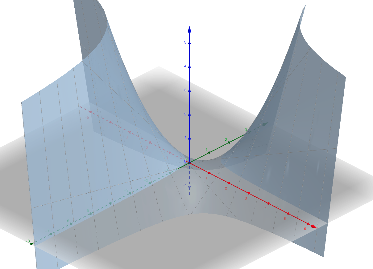
Figure 4: Saddle surface

Let the objective function be :

$$G^{L}(p_{1},p_{2})=p_{1}p_{2}-(a^{L}p_{1}+b^{L}p_{2}+c^{L})$$ (13)

To find the appropriate parameters, we need find the optimal value of $a^{L}$, $b^{L}$ and $c^{L}$ to minimize the gap function $G$, $minG^{L}(p_{1},p_{2})$. As the $p_{1}$ and $p_{2}$ are constrained by the area $[l_{1},u_{1}]\times[l_{2},u_{2}]$. The objective function can be reformulated as:

$$\mathop{max}\limits_{a^{L},b^{L},c^{L}}F^{L}(p_{1},p_{2})=\mathop{max}\limits_{a^{L},b^{L},c^{L}}\int_{p_{1}\in\left[l_{1},u_{1}\right]}\int_{p_{2}\in\left[l_{2},u_{2}\right]}a^{L}p_{1}+b^{L}p_{2}+c^{L}$$ (14)

s.t. $G^{L}(p_{1},p_{2})\geq 0\text{ }(\forall(p_{1},p_{2})\in\left[l_{1},u_{1}\right]\times\left[l_{2},u_{2}\right])$.

First, we need to ensure that $G^{L}(p_{1},p_{2})\geq 0$ by finding the minimum value of $G(p_{1},p_{2})$. The first-order partial derivatives of $G^{L}$ are: $\frac{\partial G^{L}}{\partial p_{1}}=p_{2}-a^{L},\frac{\partial G^{L}}{\partial p_{2}}=p_{1}-b^{L}$. The critical points are $\frac{\partial G^{L}}{\partial p_{1}}=0$ and $\frac{\partial G^{L}}{\partial p_{2}}=0$, which leads to $p_{2}=a^{L}$ and $p_{1}=b^{L}$. Then we form the Hessian matrix to justify the behavior of the critical points:

$$\mathrm{H}(G^{L}(p_{1},p_{2}))=\left(\begin{array}[]{cc}\frac{\partial^{2}G^{L}}{\partial p_{1}^{2}}&\frac{\partial^{2}G^{L}}{\partial p_{1}\partial p_{2}}\\ \frac{\partial^{2}G^{L}}{\partial p_{2}\partial p_{1}}&\frac{\partial^{2}G^{L}}{\partial p_{2}^{2}}\end{array}\right)=\left(\begin{array}[]{cc}0&1\\ 1&0\end{array}\right)$$ (15)

Then we compute the Hessian:

$$\operatorname{det}\mathrm{H}(G^{L}(p_{1},p_{2}))=\left(\frac{\partial^{2}G^{L}}{\partial p_{1}^{2}}\right)\left(\frac{\partial^{2}G^{L}}{\partial p_{2}^{2}}\right)-\frac{\partial^{2}G^{L}}{\partial p_{1}\partial p_{2}}=-1<0$$ (16)

Thus, the critical points are saddle points, which can be illustrated in Figure 4. Thus, the minimum value of $G^{L}(p_{1},p_{2})$ can be found on the boundary. As there exists a point $(p_{1}^{0},p_{2}^{0})\text{}\in[l_{1},u_{1}]\times[l_{2},u_{2}]$ such that $G^{L}(p_{1}^{0},p_{2}^{0})=0$. Thereby, we need to satisfy constraints on $G^{L}(p_{1},p_{2})$ that $G^{L}(p_{1}^{0},p_{2}^{0})=0$ and the value of $G^{L}$ on boundary points: $G^{L}(l_{1},u_{1}),G^{L}(l_{1},u_{2}),G^{L}(l_{2},u_{1}),G^{L}(l_{2},u_{2})\geq 0$. Equivalently, this can be formulated as:

$$\left\{\begin{array}[]{c}c=p_{1}^{0}p_{2}^{0}-a^{L}p_{1}^{0}-b^{L}p_{2}^{0}\\ l_{1}l_{2}-a^{L}\left(l_{1}-p_{1}^{0}\right)-b^{L}\left(l_{1}-p_{2}^{0}\right)-p_{1}^{0}p_{2}^{0}\geq 0\\ l_{1}u_{2}-a^{L}\left(l_{1}-p_{1}^{0}\right)-b^{L}\left(u_{2}-p_{2}^{0}\right)-p_{1}^{0}p_{2}^{0}\geq 0\\ u_{1}l_{2}-a^{L}\left(u_{1}-p_{1}^{0}\right)-b^{L}\left(l_{2}-p_{2}^{0}\right)-p_{1}^{0}p_{2}^{0}\geq 0\\ u_{1}u_{2}-a^{L}\left(u_{1}-p_{1}^{0}\right)-b^{L}\left(u_{2}-p_{2}^{0}\right)-p_{1}^{0}p_{2}^{0}\geq 0\end{array}\right.$$ (17)

By substituting the $c^{L}$ in Eq. 13 with equation Eq. 17, we can obtain:

$$F^{L}(p_{1},p_{2})=\Lambda[(l_{1}+u_{1}-2p_{1}^{0})a^{L}+(l_{2}+u_{2}-2p_{2})b^{L}+2p_{1}^{0}p_{2}^{0}],$$ (18)

where $\Lambda=\frac{(u_{1}-l_{1})(u_{2}-l_{2})}{2}$. As the minimum value can only be found on the boundary, the $p_{1}^{0}$ can be $l_{1}$ or $u_{1}$.

• If $p_{1}^{0}=l_{1}$: By substituting it in Eq. 17 and Eq. 18 , we get:

  $$\left\{\begin{array}[]{c}a^{L}\leq\frac{u_{1}l_{2}-l_{1}p_{2}^{0}-b^{L}\left(l_{2}-p_{2}^{0}\right)}{u_{1}-l_{1}},a^{L}\leq\frac{u_{1}u_{2}-l_{1}p_{2}^{0}-b^{L}\left(u_{2}-p_{2}^{0}\right)}{u_{1}-l_{1}},l_{1}\leq b^{L}\leq l_{1}\Leftrightarrow b^{L}=l_{1}.\\ F^{L}(p_{1},p_{2})=\Lambda[(u_{1}-l_{1})a^{L}+(l_{2}+u_{2}-2p_{2}^{0})b^{L}+2l_{1}p_{2}^{0}].\end{array}\right.$$ (19)

  Next, replacing $b^{L}=l_{1}$, we can obtain:

  $$\left\{\begin{array}[]{c}F^{L}(p_{1},p_{2})=\Lambda[(u_{1}-l_{1})a^{L}+l_{1}(l_{2}+u_{2})],\\ \left(u_{1}-l_{1}\right)a^{L}\leq-l_{1}p_{2}^{0}+\min\left(u_{1}l_{2}-b^{L}\left(l_{2}-p_{2}^{0}\right),u_{1}u_{2}-b^{L}\left(u_{2}-p_{2}^{0}\right)\right)=\left(u_{1}-l_{1}\right)l_{2}.\end{array}\right.$$

  As a result, we obtain $a^{L}\leq l_{2}$. To maximize $F^{L}(p_{1},p_{2})$, because $\Lambda\geq 0$, we adapt $a^{L}=l_{2}$ to get $F^{L}(p_{1},p_{2})=\Lambda(u_{1}l_{2}+l_{1}u_{2})$, which is constant.

• If $p_{1}^{0}=u_{1}$:Similarly, we can compute

  $$\left\{\begin{array}[]{c}a^{L}\geq\frac{l_{1}l_{2}-u_{1}p_{2}^{0}-b^{L}\left(l_{2}-p_{2}^{0}\right)}{l_{1}-u_{1}},\begin{array}[]{c}a^{L}\geq\frac{l_{1}u_{2}-u_{1}p_{2}^{0}-b^{L}\left(u_{2}-p_{2}^{0}\right)}{l_{1}-u_{1}},u_{1}\leq b^{L}\leq u_{1}\Leftrightarrow b^{L}=u_{1}\end{array}.\\ F^{L}(p_{1},p_{2})=\Lambda\left[\left(l_{1}-u_{1}\right)a^{L}+\left(l_{2}+u_{2}-2p_{2}^{0}\right)b^{L}+2u_{1}p_{2}^{0}\right]\end{array}\right.$$

  By replacing $b^{L}=u_{1}$, we obtain

  $$\left\{\begin{array}[]{c}F^{L}(p_{1},p_{2})=\Lambda\left[\left(l_{1}-u_{1}\right),a^{L}+u_{1}\left(l_{2}+u_{2}\right)\right],\\ \left(l_{1}-u_{1}\right)a^{L}\leq-u_{1}p_{2}^{0}+\min\left(l_{1}l_{2}-b^{L}\left(l_{2}-p_{2}^{0}\right),l_{1}u_{2}-b^{L}\left(u_{2}-p_{2}^{0}\right)\right)=\left(l_{1}-u_{1}\right)u_{2}\end{array}\right.$$

  Then, we conclude that $a^{L}\geq u_{y}$, and $F^{L}=\Lambda(l_{1}u_{2}+u_{1}l_{2})$

As the $F^{L}$ are the same for above two cases, which is not determined by $p_{2}^{0}$, we can choose $p_{2}^{0}=l_{2}$. Thus we can obtain the parameters to compute the lower bounds: $a^{L}=l_{2},b^{L}=l_{1},c^{L}=-l_{1}l_{2}$

B.2 derivation for the upper bound

Similarly, to compute the upper bound, we can formulate the $G^{U}(p_{1},p_{2})$ as:

$$G^{U}(p_{1},p_{2})=(a^{U}p_{1}+b^{U}p_{2}+c^{U})-p_{1}p_{2}$$ (20)

Thus, the objective function to compute the upper bound is:

$$\mathop{min}\limits_{a^{U},b^{U},c^{U}}F^{U}(p_{1},p_{2})=\mathop{min}\limits_{a^{U},b^{U},c^{U}}\int_{p_{1}\in\left[l_{1},u_{1}\right]}\int_{p_{2}\in\left[l_{2},u_{2}\right]}a^{U}p_{1}+b^{U}p_{2}+c^{U},$$ (21)

and then it can be expressed as:

$$F^{U}(p_{1},p_{2})=\Lambda[(l_{1}+u_{1}-2p_{1}^{0})a^{U}+(l_{2}+u_{2}-2p_{2})b^{U}+2p_{1}^{0}p_{2}^{0}],\Lambda=\frac{(u_{1}-l_{1})(u_{2}-l_{2})}{2}$$

• If we set $p_{1}^{0}=l_{1}$:

  $$\left\{\begin{array}[]{c}a^{U}\geq\frac{u_{1}l_{2}-l_{1}p_{2}^{0}-b^{U}\left(l_{2}-p_{2}^{0}\right)}{u_{1}-l_{1}},a^{U}\geq\frac{u_{1}u_{2}-l_{1}p_{2}^{0}-b^{U}\left(u_{2}-p_{2}^{0}\right)}{u_{1}-l_{1}},l_{1}\leq b^{U}\leq l_{1}\Leftrightarrow b^{U}=l_{1}.\\ F^{U}(p_{1},p_{2})=\Lambda[(u_{1}-l_{1})a^{U}+(l_{2}+u_{2}-2p_{2}^{0})b^{U}+2l_{1}p_{2}^{0}]\end{array}\right.$$

  After substituting $b^{U}=l_{1}$, we get

  $$\left\{\begin{array}[]{c}F^{U}(p_{1},p_{2})=\Lambda[(u_{1}-l_{1})a^{U}+l_{1}(l_{2}+u_{2})],\\ \left(u_{1}-l_{1}\right)a^{U}\geq-l_{1}p_{2}^{0}+\max\left(u_{1}l_{2}-b^{U}\left(l_{2}-p_{2}^{0}\right),u_{1}u_{2}-b^{U}\left(u_{2}-p_{2}^{0}\right)\right)=\left(u_{1}-l_{1}\right)u_{2}\end{array}\right.$$

  Thus, $a^{U}\geq u_{2}$. To minimize $F^{U}(p_{1},p_{2})$, we adapt $a^{U}=u_{2}$ to get $F^{U}(p_{1},p_{2})=\Lambda(l_{1}l_{2}+u_{1}u_{2})$.

• If we set $p_{1}^{0}=l_{1}$:

  $$\left\{\begin{array}[]{c}a^{U}\leq\frac{l_{1}l_{2}-u_{1}p_{2}^{0}-b^{U}\left(l_{2}-p_{2}^{0}\right)}{l_{1}-u_{1}},a^{U}\leq\frac{l_{1}u_{2}-u_{1}p_{2}^{0}-b^{U}\left(u_{2}-p_{2}^{0}\right)}{l_{1}-u_{1}},u_{1}\leq b^{U}\leq u_{1}\Leftrightarrow b^{U}=u_{1}\\ F^{U}(p_{1},p_{2})=\Lambda\left[\left(l_{1}-u_{1}\right)a^{U}+\left(l_{2}+u_{2}-2p_{2}^{0}\right)b^{U}+2u_{1}p_{2}^{0}\right]\end{array}\right.$$

  Next, we get

  $$\left\{\begin{array}[]{c}F^{U}(p_{1},p_{2})=\Lambda\left[\left(l_{1}-u_{1}\right)a^{U}+u_{1}\left(l_{2}+u_{2}\right)\right],\\ \left(l_{1}-u_{1}\right)a^{U}\leq-u_{1}p_{2}^{0}+\max\left(l_{1}l_{2}-b^{U}\left(l_{2}-p_{2}^{0}\right),l_{1}u_{2}-b^{U}\left(u_{2}-p_{2}^{0}\right)\right)=\left(l_{1}-u_{1}\right)l_{2}\end{array}\right.$$

  Thus, we can conclude that $a^{U}\leq l_{2}$, and to minimize $F^{U}$, we set $a^{U}=l_{2}$ to form $F^{U}=\Lambda(l_{1}l_{2}+u_{1}u_{2})$.

As the two results for $F^{U}$ are the same, we choose $p_{2}^{0}=l_{2}$ to obtain the final parameters for the upper bound: $a^{U}=u_{2},b^{U}=l_{1},c^{U}=-l_{1}u_{2}$.

Appendix C Extra Experiments

As computing the bounds by 3DCertify is computationally unattainable, it will terminate after verifying several samples. Thus, we present the results to verify 10 samples. From the table 4, we can see that our method could obtain tighter bounds and significantly reduce the time.

no. points	Pooling	Acc.	N	$l_{p}$	Certified Bounds				Our vs.		Attack
					Our		3DCertify		3DCertify (%)		CW	PGD
					ave	time(s)	ave	time(s)	ave	time	ave	ave
512	Max	82.12	9	$l_{\infty}$*	0.0052	58.31	0.0030	487.21	+73.33	-88.03	0.0325	0.0174
				$l_{2}$	0.0159	58.78	-	-	-	-	0.2627	0.3583
				$l_{1}$	0.0196	54.34	-	-			4.4918	5.0793
1024	Average	72.61	5	$l_{\infty}$*	0.0141	50.05	0.0107	472.15	+31.77	-89.4	0.0512	0.0391
				$l_{2}$	0.0471	21.88	-	-	-	-	0.4635	0.3877
				$l_{1}$	0.0544	10.08	-	-			2.3798	3.0146

Table 4: Average bounds and computational times on PointNet models without JANet. For the certified bounds, the higher the better. The bounds obtained by attack based method can be viewed as upper bounds.

4 Configuration of Various PointNet models

Below are the specific layer configurations for 13-layer full PointNet with JANet and PointNets without JANet.

No	Type	no. features	normalization	activation function
1	Conv1D	32	BatchNormalization	ReLU
2	Conv1D	64	BatchNormalization	ReLU
3	Conv1D	512	BatchNormalization	ReLU
4	GlobalMaxpooling
5	Dense	256	BatchNormalization	ReLU
6	Dense	512	BatchNormalization	ReLU
	Reshape
	Multiplication

Table 5: Configuration for T-Net.

No	Type	no. features	normalization	activation function
	T-Net
7	Conv1D	32	BatchNormalization	ReLU
8	Conv1D	64	BatchNormalization	ReLU
9	Conv1D	512	BatchNormalization	ReLU
10	GlobalMaxpooling
11	Dense	512	BatchNormalization	ReLU
12	Dense	256	BatchNormalization	ReLU
	Dropout

Table 6: Configuration for full PointNet with JANet.

No	Type	no. features	normalization	activation function
1	Conv1D	32	BatchNormalization	ReLU
2	Conv1D	32	BatchNormalization	ReLU
3	Conv1D	64	BatchNormalization	ReLU
4	Conv1D	512	BatchNormalization	ReLU
5	GlobalMaxpooling
6	Dense	512	BatchNormalization	ReLU
7	Dense	256	BatchNormalization	ReLU
	Dropout

Table 7: Configuration for 7-layer PointNet without JANet.

No	Type	no. features	normalization	activation function
1	Conv1D	32	BatchNormalization	ReLU
2	Conv1D	32	BatchNormalization	ReLU
3	Conv1D	64	BatchNormalization	ReLU
4	Conv1D	64	BatchNormalization	ReLU
5	Conv1D	512	BatchNormalization	ReLU
6	Conv1D	512	BatchNormalization	ReLU
7	GlobalMaxpooling
8	Dense	512	BatchNormalization	ReLU
9	Dense	256	BatchNormalization	ReLU
10	Dense	256	BatchNormalization	ReLU
11	Dense	128	BatchNormalization	ReLU
12	Dense	128	BatchNormalization	ReLU
	Dropout

Table 8: Configuration for 12-layer PointNet without JANet.

Statements and Declarations

4.1 Funding

This work is supported by Partnership Resource Fund on EPSRC project on Offshore Robotics for Certification of Assets (ORCA) [EP/R026173/1].

4.2 Conflict/Competing of interest interests

The authors declare that they have no conflict of interest

4.3 Ethics approval $\&$ Consent to participate/publication

Not applicable.

4.4 Code/Data availability

Our code is available on https://github.com/TrustAI/3DVerifier.

4.5 Authors’ contributions

RM contributed to the idea, algorithm, theoretical analysis, writing, and experiments. WR contributed to the idea, theoretical analysis, and writing. LM contributed to the theoretical analysis and writing. QN contributed to the idea and writing.

References

- \bibcommenthead
- Aoki et al (2019) Aoki Y, Goforth H, Srivatsan RA, et al (2019) Pointnetlk: Robust & efficient point cloud registration using pointnet. CVPR
- Athalye et al (2018) Athalye A, Carlini N, Wagner D (2018) Obfuscated gradients give a false sense of security: Circumventing defenses to adversarial examples. ICML
- Boopathy et al (2019) Boopathy A, Weng TW, Chen PY, et al (2019) CNN-Cert: An Efficient Framework for Certifying Robustness of Convolutional Neural Networks. AAAI
- Bunel et al (2017) Bunel R, Turkaslan I, Torr PH, et al (2017) A unified view of piecewise linear neural network verification. arXiv
- Cao et al (2019) Cao Y, Xiao C, Yang D, et al (2019) Adversarial objects against lidar-based autonomous driving systems. arXiv
- Carlini and Wagner (2017) Carlini N, Wagner D (2017) Towards evaluating the robustness of neural networks. SP
- Chen et al (2017) Chen X, Ma H, Wan J, et al (2017) Multi-view 3D object detection network for autonomous driving. CVPR
- Chen et al (2021) Chen X, Jiang K, Zhu Y, et al (2021) Individual tree crown segmentation directly from uav-borne lidar data using the pointnet of deep learning. Forests
- Dvijotham et al (2018) Dvijotham K, Stanforth R, Gowal S, et al (2018) A dual approach to scalable verification of deep networks. UAI
- Gehr et al (2018) Gehr T, Mirman M, Drachsler-Cohen D, et al (2018) Ai2: Safety and robustness certification of neural networks with abstract interpretation. SP
- Goodfellow et al (2014) Goodfellow IJ, Shlens J, Szegedy C (2014) Explaining and harnessing adversarial examples. arXiv
- Jin et al (2020) Jin G, Yi X, Zhang L, et al (2020) How does weight correlation affect generalisation ability of deep neural networks? NeurIPS
- Jin et al (2022) Jin G, Yi X, Huang W, et al (2022) Enhancing adversarial training with second-order statistics of weights. In: CVPR
- Katz et al (2017) Katz G, Barrett C, Dill DL, et al (2017) Reluplex: An efficient SMT solver for verifying deep neural networks. ICCAV
- Kurakin et al (2016) Kurakin A, Goodfellow IJ, Bengio S (2016) Adversarial examples in the physical world. arXiv
- Lee et al (2020) Lee K, Chen Z, Yan X, et al (2020) ShapeAdv: Generating Shape-Aware Adversarial 3D Point Clouds. arXiv
- Liang et al (2018) Liang M, Yang B, Wang S, et al (2018) Deep continuous fusion for multi-sensor 3d object detection. ECCV
- Liu et al (2019) Liu D, Yu R, Su H (2019) Extending adversarial attacks and defenses to deep 3D point cloud classifiers. ICIP
- Lorenz et al (2021) Lorenz T, Ruoss A, Balunović M, et al (2021) Robustness certification for point cloud models. arXiv
- Paigwar et al (2019) Paigwar A, Erkent O, Wolf C, et al (2019) Attentional pointnet for 3d-object detection in point clouds. CVPR Workshops
- Qi et al (2017a) Qi CR, Su H, Mo K, et al (2017a) PointNet: Deep Learning on Point Sets for 3D Classification and Segmentation. CVPR
- Qi et al (2017b) Qi CR, Yi L, Su H, et al (2017b) PointNet++: Deep Hierarchical Feature Learning on Point Sets in a Metric Space. arXiv
- Salman et al (2019) Salman H, Yang G, Zhang H, et al (2019) A convex relaxation barrier to tight robustness verification of neural networks. arXiv
- Shi et al (2020) Shi Z, Zhang H, Chang KW, et al (2020) Robustness Verification for Transformers. ICLR
- Singh et al (2019) Singh G, Gehr T, Püschel M, et al (2019) An abstract domain for certifying neural networks. ACM PL
- Stets et al (2017) Stets JD, Sun Y, Corning W, et al (2017) Visualization and Labeling of Point Clouds in Virtual Reality. SIGGRAPH Asia
- Sun et al (2020) Sun J, Koenig K, Cao Y, et al (2020) On Adversarial Robustness of 3D Point Cloud Classification under Adaptive Attacks. arXiv
- Szegedy et al (2014) Szegedy C, Zaremba W, Sutskever I, et al (2014) Intriguing properties of neural networks. ICLR
- Tjeng et al (2018) Tjeng V, Xiao KY, Tedrake R (2018) Evaluating robustness of neural networks with mixed integer programming. ICLR
- Tramer et al (2020) Tramer F, Carlini N, Brendel W, et al (2020) On adaptive attacks to adversarial example defenses. arXiv
- Varley et al (2017) Varley J, DeChant C, Richardson A, et al (2017) Shape completion enabled robotic grasping. IROS
- Wang et al (2018) Wang S, Pei K, Whitehouse J, et al (2018) Efficient formal safety analysis of neural networks. arXiv
- Weng et al (2018) Weng L, Zhang H, Chen H, et al (2018) Towards Fast Computation of Certified Robustness for ReLU Networks. ICML
- Wicker and Kwiatkowska (2019) Wicker M, Kwiatkowska M (2019) Robustness of 3D deep learning in an adversarial setting. CVPR
- Wong and Kolter (2018) Wong E, Kolter Z (2018) Provable defenses against adversarial examples via the convex outer adversarial polytope. ICML
- Wu et al (2015) Wu Z, Song S, Khosla A, et al (2015) 3D ShapeNets: A Deep Representation for Volumetric Shapes. CVPR
- Xiang et al (2019) Xiang C, Qi CR, Li B (2019) Generating 3D adversarial point clouds. CVPR
- Zhang et al (2018) Zhang H, Weng TW, Chen PY, et al (2018) Efficient neural network robustness certification with general activation functions. ANIPS
- Zhang et al (2019a) Zhang Q, Yang J, Fang R, et al (2019a) Adversarial attack and defense on point sets. arXiv
- Zhang et al (2019b) Zhang Y, Liang G, Salem T, et al (2019b) Defense-pointnet: Protecting pointnet against adversarial attacks. ICBD
- Zhao et al (2020) Zhao Y, Wu Y, Chen C, et al (2020) On isometry robustness of deep 3D point cloud models under adversarial attacks. CVPR
- Zhou et al (2019) Zhou H, Chen K, Zhang W, et al (2019) Dup-net: Denoiser and upsampler network for 3D adversarial point clouds defense. ICCV