Communication-Efficient Diffusion Strategy for Performance Improvement of Federated Learning with Non-IID Data

Abstract

Federated learning (FL) is a novel learning paradigm that addresses the privacy leakage challenge of centralized learning. However, in FL, users with non-independent and identically distributed (non-IID) characteristics can deteriorate the performance of the global model. Specifically, the global model suffers from the weight divergence challenge owing to non-IID data. To address the aforementioned challenge, we propose a novel diffusion strategy of the machine learning (ML) model (FedDif) to maximize the FL performance with non-IID data. In FedDif, users spread local models to neighboring users over D2D communications. FedDif enables the local model to experience different distributions before parameter aggregation. Furthermore, we theoretically demonstrate that FedDif can circumvent the weight divergence challenge. On the theoretical basis, we propose the communication-efficient diffusion strategy of the ML model, which can determine the trade-off between the learning performance and communication cost based on auction theory. The performance evaluation results show that FedDif improves the test accuracy of the global model by 10.37% compared to the baseline FL with non-IID settings. Moreover, FedDif improves the number of consumed sub-frames by 1.28 to 2.85 folds to the latest methods except for the model compression scheme. FedDif also improves the number of transmitted models by 1.43 to 2.67 folds to the latest methods.

I Introduction

As interests in the privacy of user data emerge, and a novel distributed learning paradigm has been proposed for users to participate in the training process. Federated learning (FL) is a representative method for training the machine learning (ML) model without leaking users’ privacy [1]. It preserves the privacy of user data via two procedures: local training and global aggregation. Specifically, a central server distributes the global model to users, and users train the local model using their private data (local training). Furthermore, the central server collects local models from users and updates the global model (global aggregation). Global aggregation is an essential part of FL for capturing both advantages of maintaining the learning performance and preserving user data privacy. Through the procedures of FL, the privacy of user data can be protected because eavesdroppers or honest-but-curious servers cannot infer users’ private data but solely collect parameters.

Although FL can protect users’ data privacy in training, it still faces a crucial issue when training user data. The abnormal user data may degrade the learning performance by disturbing the training of the ML model. While the central server can directly curate a training dataset in centralized learning, it cannot manage the data of each user in FL. Specifically, in FL, malicious or non-independent and identically distributed (non-IID) data can incur severe performance degradation as abnormal data. Regarding malicious data injection, adversaries can manipulate the result of the global model by exploiting the characteristics of FL [2]. Several studies based on advanced security techniques such as differential privacy, adversary detection, and down-weighting are proposed to prevent malicious data injection [3, 4].

Performance degradation by non-IID user data may be a severer issue in FL. When users train the local model with their non-IID data, it may cause performance degradation of the global model regardless of any intention [5]. In particular, training a local model with non-IID data may induce the over-fitted local model, and the biased parameters of the local model may permeate into the global model. Consequently, the global aggregation of biased models may lead to weight divergence of the global model [6, 7]. Reducing the weight divergence of the global model is crucial to maintain the learning performance in FL. Several studies have been proposed to reduce biases that occurred by non-IID data [6, 8, 9]. These studies facilitate addressing the performance degradation challenges by non-IID data. However, issues at another facet, such as additional privacy leakage, weight divergence, and prolonged training time, remain open.

This study presents a novel diffusion strategy of machine learning models called FedDif to improve the performance of a global model with non-IID data and minimize the required communication rounds. First, we discover some insights for designing FedDif by discussing the following question: “Is it possible to obtain the same effect of training the IID data by training the local models with multiple non-IID data before global aggregation?” We re-think the general concept of FL that the user trains the ML model to the fact that the model learns the different users’ data. In FedDif, each user is considered as non-IID batch data, and models learn various non-IID data by passing through multiple users before global aggregation. User data have non-IID characteristics because they are personalized and biased to a particular class. Therefore, we propose the diffusion mechanism in which users relay models to train more diverse data to models. Consequently, we can achieve a similar effect as the model trains IID data via enough diffusion iterations.

Although the diffusion mechanism can mitigate the effects of the non-IID data, excessive diffusion may substantially increase the total training time and deteriorate the performance of the communication system. In other words, there is a trade-off between improving learning performance and minimizing communication costs. To analyze the communication cost of the diffusion mechanism, we consider two types of communication resources: frequency and time domain resources. Immoderate diffusion can deteriorate the network performance because users can over-occupy bandwidth for sending their model. Adversely, passive diffusion can require more time-domain resources to achieve the targeted performance. Thus, an efficient scheduling method should be designed for the communication-efficient diffusion mechanism by reducing the required communication resources and training time.

We first construct an optimization problem to find the optimal scheduling policy for FedDif by introducing two variables: IID distance and communication cost. IID distance represents how much is the learned data distribution of the model uniformly distributed. Then, we provide the theoretical analysis of the diffusion mechanism by demonstrating that the diffusion mechanism can mitigate weight divergence. Moreover, our analysis provides a guideline for optimization by demonstrating that the scheduling policy should assign the next users who can minimize the IID distance of models. Finally, we propose the diffusion strategy to find a feasible solution for the optimization problem based on the auction theory.

Our contributions are summarized as follows:

• We introduce a novel diffusion mechanism of ML models called FedDif to reduce the weight divergence due to non-IID data. In the diffusion mechanism, before the global aggregation, each local model accumulates the personalized data distributions of different users and obtains a similar effect to train IID data.

• We design the diffusion strategy based on auction theory to determine the compromise between improving the learning performance and reducing the communication cost. We construct the optimization problem to find the trade-off. The auction provides a feasible solution for the optimization problem to BS based on the proposed winner selection algorithm.

• We provide a theoretical analysis of FedDif by two propositions to demonstrate that the diffusion mechanism can mitigate the weight divergence. Propositions show that the IID distance is closely related to the weight divergence and that the diffusion mechanism can minimize the IID distance of the model after enough diffusion.

• We further empirically demonstrate that FedDif can improve the performance of the global model and communication efficiency via simulations. It can be seen that FedDif increases the test accuracy of the global model with minimum communication cost than other previous methods. Moreover, we provide our implementations of FedDif on an open-source platform.

The rest of this paper is organized as follows. Section II introduces related works. Section III provides the system model and problem formulation. Section IV proposes FedDif based on auction theory. Sections V and VI present the theoretical and experimental analysis of FedDif, respectively. Finally, we present our conclusions in Section VII.

II Related works

Recent advances in FL have focused on efficiency improvement of the training process, defense against various attacks, and training under the heterogeneous environment of users [10]. In particular, studies on training under the heterogeneous environment of users, such as training with non-IID user data, have recently become one of the most crucial issues on FL owing to the personalized user data. The cooperative FL is a representative method to train various personalized data and improve the efficiency of FL. The communication efficiency of FL is also considered because the server and users are obliged to exchange the ML model. In this section, we will introduce the previous works on FL with non-IID data, cooperative FL, and communication-efficient FL, which are the aim of our proposed strategy in this paper.

II-1 Federated learning with non-IID data

Several studies have investigated the effect of the heterogeneous environment of users on the performance of FL [6, 7]. Specifically, the non-IID user data, called statistical heterogeneity, may significantly decline its learning performance owing to several causes, such as weight divergence and gradient exploding. Zhao et al. [6] theoretically demonstrated that the earth mover’s distance (EMD) between users’ non-IID data and the population distribution causes the weight divergence. Moreover, the authors proposed a data-sharing strategy. In wireless networks, the authors of the study [7] practically analyzed the performance of FL with non-IID data. In [9], the authors proposed the data augmentation scheme in which user data is formed as IID based on the generative model. The authors of [11] proposed the fine-tuning scheme of the global model based on shared user data. However, the privacy leakage of user data and costly communications on the data-sharing schemes still exist.

Weight regularization and calibration can provide a clue to addressing the non-IID problem without data-sharing[8, 12, 13]. These studies mitigate the effect of non-IID data in the global model by adaptively adjusting the weight of the local model based on the weight regularization techniques. They can internally improve the performance of the global model in FL with non-IID data without any interactions among users. Adversely, our proposed FedDif focuses on exchanging knowledge of the different user datasets among the local model by diffusing the model in wireless networks. Thus, FedDif can externally improve the performance of FL in synergy with the weight regularization methods.

Other studies that can externally improve the performance of FL with non-IID data exist as user selection and model selection[14, 15, 16, 17]. In [14, 15], the authors focused on selecting users that can reduce biases due to non-IID data. The study [16] proposed a user grouping scheme that divides users into several groups managed by mediators. The authors of [17] proposed the model selection scheme that deletes models degraded by non-IID data and cloning well-trained models. Those studies can externally reduce biases by non-IID data. Furthermore, our proposed FedDif can improve the performance of FL by collaborating with the user and model selection schemes.

II-2 Cooperative federated learning

Cooperative FL is another method of training to remove the aggregation server, i.e., the decentralized FL, or exchange the local model between users. Several studies attempted to discover the effect of the decentralized FL[18, 19]. The decentralized FL can reduce the risk of a single point of failure that can occur by the outage of the aggregation server. These can enhance the robustness of FL and create a synergy effect with our proposed FedDif.

Other studies of cooperative FL proposed exchanging the local model between users [20, 21, 22, 23]. These can improve the performance of FL by training the private data of different users before aggregation. Chiu et al. [20] proposed a novel operation called FedSwap, which randomly re-distributes local models to users to train the multiple non-IID data before aggregation. Lin et al. [21] proposed two-timescale hybrid federated learning (TT-HF) that aggregates the model in local clusters and cooperatively trains the model in each local cluster. The authors of [22] proposed consensus-based federated averaging (CFA) that trains the ML model by the consensus-based in-network FL between different users via D2D communications. The authors employ the negotiation step of the diffusion strategy to make a consensus. The authors of [23] investigated several methods of decentralized FL. The diffusion algorithm is considered to exchange information about how neighbor models should be adjusted considering local data. Moreover, the authors claimed that exploring the trade-off between the convergence speed and the cost of large communication overhead is currently an open challenge.

II-3 Communication-efficient federated learning

Unlike centralized learning, FL should consider the communication costs such as transmission time or consistency. Such communication costs may influence the learning performance of the ML model and training time. Several studies on communication-efficient FL demonstrate the importance of communication efficiency in FL [24, 25, 26, 27]. In [24], the authors proposed a D2D-assisted hierarchical federated learning scheme that significantly reduces the traffic load via D2D grouping and master user selection in the group. The studies [25, 26] proposed the communication-efficient FL by considering the energy consumption and transmission model. In IoT systems, Mills et al. [27] proposed a communication-efficient Federated Averaging (CE-FedAvg) scheme adapted with distributed Adam optimization and compression methods.

To date, the aforementioned studies on FL with non-IID data have improved the performance of the global model and clarified the reason for the weight divergence. We further propose the universal strategy of training the ML model in FL by considering the cumulative experience of user data for the ML model and communication costs for diffusion.

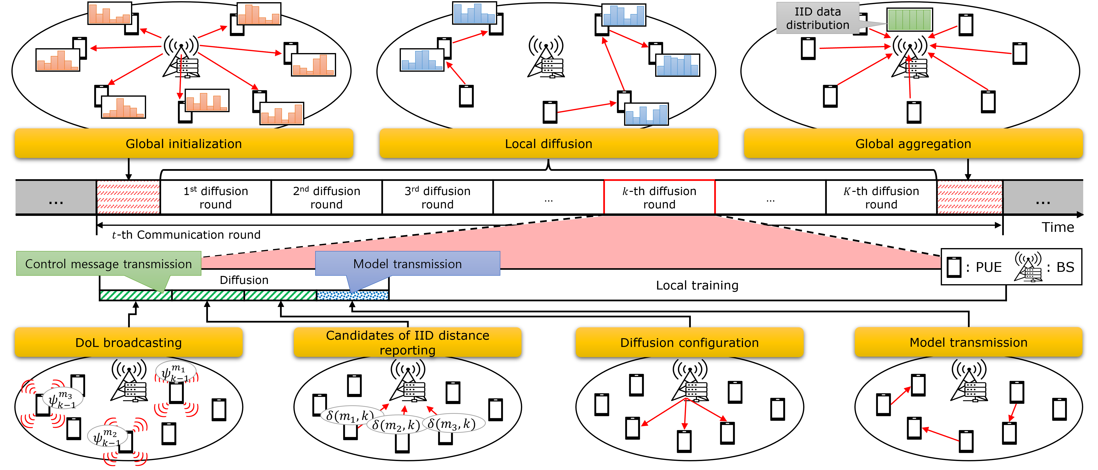
Figure 1: Overview of FedDif.

III System model and problem formulation

This section describes the system model FedDif operates (Section III-A) and the representations of data distribution (Section III-B). Then, we formulate the optimization problem for finding the trade-off between learning performance and communication cost (Section III-C).

III-A System description

We consider the typical federated learning frameworks over wireless networks consisting of a base station (BS) and user equipment (UE). Assuming that $T$ communication rounds are required to train the global model sufficiently, the BS first selects the available UE subset to prevent the failure of training the global model by the outage of the UE. We define a subset of $N_{P}$ available UEs as the participating UE (PUE) set $\mathcal{N}_{P}=\{1,...,N_{P}\}$. UEs not participating in the training compose the cellular UE (CUE) set $\mathcal{N}_{C}=\{1,...,N_{C}\}$. The BS distributes the global model $\textbf{w}_{t-1}^{(g)}$ consisting of parameters of the global model in the $(t-1)$-th communication round to PUEs. $\mathcal{M}$ is a set of distributed models called the local model, and $m\in\mathcal{M}$ is the local model with the parameters $\textbf{w}_{t,0}^{(m)}$ replicated by the global model. Local models are independent of PUEs in FedDif, and each PUE is considered as a single batch data.

Unlike the typical FL, in FedDif, PUEs diffuse models to neighbor PUEs before global aggregation as illustrated in Fig. 1. We define one iteration of diffusion as the diffusion round. In the $k$-th diffusion round, each PUE $i$ trains the local model $\textbf{w}_{t,k}^{(m)}$ using their private dataset $\mathcal{D}_{i}$ with a size of $D_{i}$. The dataset of PUE $i$ is generated by different random variables $X_{i}$. Note that samples in each dataset are in the label space $\mathcal{C}$ whose cardinality is $C$. To define centralized learning with IID data, we consider the universal dataset comprising the dataset of all PUEs represented as $\mathcal{D}=\bigcup_{i\in\mathcal{N}_{p}}\mathcal{D}_{i}$. The total data size in the system is $D=\sum_{i\in\mathcal{N}_{P}}D_{i}$. The universal dataset is generated by a single random variable $X_{g}$. The probability density function (PDF) of random variables $X_{1},...,X_{N_{P}},X_{g}$ are denoted as $P(X_{1}),...,P(X_{N_{P}}),P(X_{g})$. We consider the relationship between PDFs of each PUE as $P(X_{i})\neq P(X_{j})$, $i,j\in\{1,...,N_{P}\}$, $i\neq j$ because each PUE’s dataset is non-IID.

We define some useful tools to analyze FedDif. The diffusion chain $\mathcal{P}_{K_{t}}^{(m)}$ is a set of PUEs that participate in the training of the model $m$, where $K_{t}$ denotes a last diffusion round of the $t$-th communication round. PUEs can be members of different diffusion chains in the entire diffusion rounds because models can require certain PUE datasets. We assume that PUEs can only participate in training the model $m$ once to avoid over-training of their data distribution and train one model at a diffusion round because of their limited computation resources. The total size of data managed by PUEs in the diffusion chain $\mathcal{P}^{(m)}_{K_{t}}$ is represented by $D_{(\mathcal{P}_{K_{t}}^{(m)})}=\sum_{i\in\mathcal{P}_{K_{t}}^{(m)}}D_{i}$. Furthermore, we define the diffusion subchain $\mathcal{P}_{k}^{(m)}\subseteq\mathcal{P}_{K_{t}}^{(m)}$, which is a set of PUEs participated in the training of the model $m$ up to the $k$-th diffusion round. The total size of data managed by PUEs in the diffusion subchain $\mathcal{P}_{k}^{(m)}$ is represented by $D_{(\mathcal{P}_{k}^{(m)})}=\sum_{i\in\mathcal{P}_{k}^{(m)}}D_{i}$. For the $k$-th diffusion round, the index of the next trainer PUE for the model $m$ in $(k-1)$-th diffusion round is represented by $i_{k}^{(m)}$, and the following relationship holds:

$$\mathcal{P}_{k}^{(m)}=\mathcal{P}_{k-1}^{(m)}\cup\{i_{k}^{(m)}\}.$$ (1)

Here, the entire trainer PUEs in the $k$-th diffusion round are represented by a vector $\mathbf{i}_{k}=\{i_{k}^{(1)},i_{k}^{(2)},...,i_{k}^{(M)}\}$.

Each PUE computes loss values for their private data batches in the local training. Let $l(\mathbf{w};x)$ denote the loss of a sample $x$ for the training of parameter $\mathbf{w}$. The expected loss function of the local model $m$ in the $t$-th communication round is the average of the expected loss of PUEs in the diffusion chain $\mathcal{P}_{K_{t}}^{(m)}$, which can be expressed as

$$\mathcal{J}(\mathbf{w}_{t,K_{t}}^{(m)}):=\frac{1}{\lvert\mathcal{P}_{K_{t}}^{(m)}\rvert}\sum_{i\in\mathcal{P}_{K_{t}}^{(m)}}\mathbb{E}_{x,y\sim P(X_{i})}[l(\mathbf{w}_{t,K_{t}}^{(m)};x)].$$ (2)

We assume that the optimization method for the diffusion mechanism is stochastic gradient descent (SGD). PUEs update the local model with their private data by SGD as

$$\begin{aligned} \mathbf{w}_{t,k}^{(m)}&=\mathbf{w}_{t,k-1}^{(m)}-\eta\triangledown\mathcal{J}(\mathbf{w}_{t,k-1}^{(m)})\\ &=\mathbf{w}_{t,k-1}^{(m)}-\frac{\eta}{\lvert\mathcal{P}_{k-1}^{(m)}\rvert}\sum_{i\in\mathcal{P}_{k-1}^{(m)}}\triangledown\mathbb{E}_{x,y\sim P(X_{i})}[l(\mathbf{w}_{t,k-1}^{(m)};x)],\end{aligned}$$ (3)

where $\eta$ denotes the learning rate. Note that all local models apply the same hyper-parameters, such as the learning rate and momentum of SGD sent by the BS.

In the case of centralized learning, the ML model is trained by the universal dataset with IID data, which follows the distribution $P(X_{g})$. The loss function with the universal dataset can be expressed by the expectation of loss function as

$$\mathcal{J}(\mathbf{w}^{(c)}_{t}):=\mathbb{E}_{x,y\sim P(X_{g})}[l(\mathbf{w}^{(c)}_{t};x)],$$ (4)

where $\mathbf{w}_{t}^{(c)}$ is the parameters of the centralized learning model in $t$-th iterations. BS updates its model based on SGD, which can be expressed as

$$\begin{aligned} \mathbf{w}_{t,k}^{(c)}&=\mathbf{w}_{t,k-1}^{(c)}-\eta\triangledown\mathcal{J}(\mathbf{w}_{t,k-1}^{(c)})\\ &=\mathbf{w}_{t,k-1}^{(c)}-\eta\triangledown\mathbb{E}_{x,y\sim P(X_{g})}[l(\mathbf{w}_{t,k-1}^{(c)};x)].\end{aligned}$$ (5)

Here, we assume that $\mathbf{w}_{t,k}^{(c)}$ is the parameters of the model after $(k+\sum_{i=1}^{t}K_{i})$ epochs.

After the local training and diffusion steps, BS aggregates the entire local model and updates the global model. The BS not only sets the training policy to all local models but also aggregates local models based on FedAvg, and can be expressed as

$$\mathbf{w}_{t}^{(g)}=\sum_{m\in\mathcal{M}}\frac{D_{(\mathcal{P}_{K_{t}}^{(m)})}}{\sum_{m^{\prime}\in\mathcal{M}}D_{(\mathcal{P}_{K_{t}}^{(m^{\prime})})}}\mathbf{w}_{t,K_{t}}^{(m)},$$ (6)

where FedAvg is a representative aggregation algorithm [1]. Based on (6), BS can aggregate local models considering the size of the training dataset of PUEs. Moreover, after sufficient diffusion rounds, the BS can obtain the global model whose performance is similar to the model trained by the universal IID dataset. This will be investigated in proposition 2 of Section V.

We should additionally consider the communication model to formulate our optimization problem and analyze FedDif. Although there are two types of communication, such as control messages and model transmissions, we assume the model transmissions as the communication cost. We employ D2D communications with overlying cellular networks in which D2D pairs equally utilize the uplink data channels with CUEs for the model transmission. To prevent the failure of securing the global model, we assume that BS distributes and collects the model at the edge of a communication round. The model transmissions may degrade the quality of the data channel in the wireless networks because the size of the ML model is primarily large. Therefore, we consider the communication costs as the required bandwidth for sending the model $m$ of $S$ bits in the model transmissions.

Let $g_{i,j}^{(k)}$ denote the channel coefficient from the transmitter $i$ to the receiver $j$ by [29, 21] as

$$g_{i,j}^{(k)}=\sqrt{\beta_{i,j}^{(k)}}h_{i,j}^{(k)}.$$ (7)

Here, the wireless channel can be attenuated by the effect of channel fading as the coefficient of small-scale fading $h_{i,j}^{(k)}$ and large-scale fading $\beta_{i,j}^{(k)}$. The small-scale fading is modeled by Rayleigh fading channel as $h_{i,j}^{(k)}\sim\mathcal{CN}(0,1)$. Large-scale fading can be modeled as

$$\beta_{i,j}^{(k)}=\beta_{0}-10\kappa\log_{10}\left(\frac{d_{i,j}^{(k)}}{d_{0}}\right)$$ (8)

where $\beta_{0}$ denotes the large-scale pathloss coefficient at a reference distance of $d_{0}$, and $\kappa$ denotes the pathloss exponent [29, 21]. We assume the overlay mode of D2D communications that D2D pairs and CUEs utilize the orthogonal radio resources, e.g., orthogonal frequency-division multiple access (OFDMA), to reduce the interference between D2D pairs. We can obtain the spectral efficiency from PUE $i$ to $j$ as follows:

$$\gamma_{i,j}^{(k)}=\log\left(1+\frac{|g_{i,j}^{(k)}|^{2}p_{i}^{(k)}}{\sigma^{2}}\right),$$ (9)

where $\sigma^{2}=\sigma_{0}B$ denotes the additive white Gaussian noise with power spectral density $\sigma_{0}$. $p_{i}$ denotes the transmit power of PUE $i$. We can finally formalize the total required bandwidth to send the model $m$ in the $k$-th diffusion round as

$$B_{k}^{(m)}=\frac{S}{\gamma_{i_{k-1}^{(m)},i_{k}^{(m)}}^{(k)}}.$$ (10)

Here, PUE $i_{k-1}^{(m)}$ sends the model $m$ to the PUE $i_{k}^{(m)}$ in $k$-th diffusion round.

III-B Representations of Data Distribution

We define a representation of the data distribution of a PUE called the data state information (DSI) vector $\mathbf{d}_{i}\sim\mathcal{D}_{i}$. Each element of the DSI is bounded in the closed interval of $[0,1]$, and the sum of all elements of the DSI is one because it indicates the ratio of data size for each class. Moreover, we represent the cumulative data distribution of the model $m$ after $k$ diffusion iterations called degree of learning (DoL) as

$$\psi_{k}^{(m)}=\frac{1}{D_{(\mathcal{P}_{k}^{(m)})}}\left(D_{(\mathcal{P}_{k-1}^{(m)})}\psi_{k-1}^{(m)}+D_{i_{k}^{(m)}}\mathbf{d}_{i_{k}^{(m)}}\right),$$ (11)

where $\mathbf{d}_{i_{k}^{(m)}}$ is the DSI of the PUE $i_{k}^{(m)}$. The DoL $\psi_{k}^{(m)}$ of the model $m$ at the $k$-th diffusion indicates the cumulative ratio of learned data size for each class in all PUEs of the diffusion subchain $\mathcal{P}_{k}^{(m)}$, and follows all properties of the DSI. We assume that the DoL of the model trained in a centralized manner with IID data follows the uniform distribution, i.e., $\mathbf{I}=\frac{1}{C}\mathbf{1}$ where $\mathbf{1}$ is a vector of all ones.

Let $\delta(\cdot)$ define the IID distance, which measures the distance between distributions of a specific probability $P$ and uniform. The Wasserstein-1, which is called Earth-mover distance, is widely used to measure the distance between two different distributions as

$$W_{1}(P_{a},P_{b})=\inf_{\gamma\in\Pi\left(P_{a},P_{b}\right)}\mathbb{E}_{\left(x,y\right)\sim\gamma}[\left\lVert x-y\right\rVert],$$ (12)

where $\Pi\left(P_{a},P_{b}\right)$ denotes the set of joint distributions of two distributions $P_{a}$ and $P_{b}$ [30]. Based on (12), we quantify the IID distance of the model $m$ in the $k$-th diffusion as follows:

$$\begin{aligned} &W_{1}\left(\psi_{k}^{(m)},\mathcal{U}\right)\\ &=\bigg{\|}\frac{1}{D_{(\mathcal{P}_{k}^{(m)})}}\left(D_{(\mathcal{P}_{k-1}^{(m)})}\psi_{k-1}^{(m)}+D_{i_{k}^{(m)}}\mathbf{d}_{i_{k}^{(m)}}\right)-\frac{1}{C}\mathbf{1}\bigg{\|},\end{aligned}$$ (13)

where $i_{k}^{(m)}$ and $\psi_{k}^{(m)}$ are the trainer PUE and DoL of the model $m$ in the $k$-th diffusion, respectively. $D_{i_{k}^{(m)}}$ and $\mathbf{d}_{i_{k}^{(m)}}$ respectively denote the data size and DSI of the PUE $i_{k}^{(m)}$. $\frac{1}{C}\mathbf{1}$ denotes the probability vector of uniform distribution $\mathcal{U}$ where $\mathbf{1}_{C}=[1,1,...,1]\in\mathbb{R}^{C}$ is one-vector of $C$-dimension.

III-C Problem formulation

There is a trade-off between the communication cost spent for the diffusion and the learning performance of the global model. For example, FedDif can require more communication resources than vanilla FL in the short term. However, in the long term, the entire iterations for obtaining the required performance of the global model may decrease because the optimization trajectory of the global model after the diffusion can become much closer to the optimal trajectory than vanilla FL. FedDif aims to coordinate the trade-off by finding the optimal diffusion chain whose PUEs maximize the decrement of IID distance and minimize the communication cost.

Two primary variables are a set of the next trainer PUEs $i_{k}^{(m)}$ and the required communication resources as $\mathbf{i}_{k}=\{i_{k}^{(m)}:m\in\mathcal{M}\}\in\mathbb{R}^{M}$ and $\mathbf{B}_{k}=\{B_{k}^{(m)}:m\in\mathcal{M}\}\in\mathbb{R}^{M}$, respectively. Note that $B_{k}^{(m)}$ denotes the total required bandwidth for the model $m$ in the $k$-th diffusion round. Then, we can define the diffusion efficiency that indicates the decrement of IID distance against the total bandwidth required to diffuse the entire models in the $k$-th diffusion round as

$$E(\textbf{i}_{k},\textbf{B}_{k})=\frac{1}{M}\sum_{m\in\mathcal{M}}\frac{\delta_{i_{k}^{(m)}}}{B_{k}^{(m)}}.$$ (14)

Here, $\delta_{i_{k}^{(m)}}$ indicates the decrement of IID distance when the next trainer PUE $i_{k}^{(m)}$ in the $k$-th diffusion round trains the model $m$ as follows:

$$\delta_{i_{k}^{(m)}}=W_{1}\left(\psi_{k-1}^{(m)},\mathcal{U}\right)-W_{1}\left(\psi_{k}^{(m)},\mathcal{U}\right),$$ (15)

where $\psi_{k}^{(m)}$ is determined by PUE $i_{k}^{(m)}$. Note that the decrement of IID distance decides the sign of the diffusion efficiency. For example, the decrement of IID distance is positive if the IID distance decrease, which means that the DoL becomes much closer to the uniform distribution. Moreover, the diffusion efficiency may decrease when the communication resources are not enough to diffuse models, or the decrement is trivial against the required resources.

Therefore, FedDif is an algorithm to solve the diffusion efficiency maximization problem by finding the optimal $\textbf{i}_{k}^{*}$ and $\textbf{B}_{k}^{*}$ as follows:

$$\max_{\textbf{i}_{k},\textbf{B}_{k}}\; E(\textbf{i}_{k},\textbf{B}_{k})$$ (16a)

s.t. $$\delta_{i_{k}^{(m)}}\geq 0,\hfill\forall i_{k}^{(m)}\in\textbf{i}_{k},$$ (16b)

$$i_{k}^{(m)}\notin\mathcal{P}_{k-1}^{(m)},\hfill\forall i_{k}^{(m)}\in\textbf{i}_{k},$$ (16c)

$$i_{k}^{(m_{1})}\neq i_{k}^{(m_{2})},\forall i_{k}^{(m_{1})},i_{k}^{(m_{2})}\in\textbf{i}_{k},$$ (16d)

$$\gamma_{i_{k-1}^{(m)},i_{k}^{(m)}}^{(k)}\geq\gamma_{\textrm{min}},\hfill\forall i_{k}^{(m)}\in\textbf{i}_{k},$$ (16e)

$$\sum_{m\in\mathcal{M}}B_{k}^{(m)}\leq B_{k}-\sum_{i\in\mathcal{N}_{C}}\tilde{B}_{k}^{(i)},\hfill\forall B_{k}^{(m)}\in\textbf{B}_{k}.$$ (16f)

Here, the constraint (16b) ensures that FedDif must not deteriorate the diffusion efficiency. Retraining the model is prohibited by constraint (16c) because it may induce weight divergence. Note that over-training the model using a single dataset can occur the weight divergence problem, namely, the overfitting problem[6]. The constraint (16d) represents that PUEs can train only one model in a diffusion round. The constraint (16e) indicates the minimum tolerable QoS requirement of PUEs. D2D communications overlying cellular networks are employed for the diffusion mechanism represented as the constraint (16f).

It can be easily seen that the diffusion efficiency maximization problem in (16) is a combinatorial optimization problem. It is difficult to obtain the solution directly because the set of feasible solutions is discrete. Therefore, based on the auction theory, we will design the diffusion strategy for finding a feasible solution that simultaneously minimizes the IID distance and required spectral resources. In the following section, we will provide a theoretical basis for the feasible solutions that can relieve the weight divergence problem and minimize IID distance.

IV Communication-efficient diffusion strategy

In this section, we introduce a novel training strategy called FedDif, which selects neighboring PUEs can maximize the diffusion efficiency and accumulates the data distributions of different PUEs by the diffusion mechanism. The aim of FedDif is to accumulate different non-IID data distributions to the local model before global aggregation.

FedDif includes four additional steps for diffusion in procedures of the typical FL, such as DoL broadcasting, candidates of IID distance reporting, diffusion configuration, and model transmission illustrated in Fig. 1. PUEs advertise the DoL $\psi_{k-1}^{(m)}$ of the responsible model $m$ to their neighboring PUEs (DoL broadcasting). Then, neighboring PUEs calculate candidate DoL of the $k$-th diffusion round for all received DoLs of the previous diffusion round using their DSI and report the candidates of IID distance to the BS (candidates of IID distance reporting). The candidates of IID distance indicate the estimated IID distance for the next diffusion round. The BS sends scheduling policies to PUEs for model transmission (Diffusion configuration). PUEs finally send their model to the next trainer PUEs via the scheduled data channel (Model transmission). We will provide the basis for how FedDif can address the performance degradation problem of FL due to the non-IID data in Section IV.

Although FedDif improves the learning performance of FL, it may become a critical issue for FedDif to require additional communication resources for diffusion. The diffusion mechanism may consume immoderate communication resources if PUEs send local models to minimize the IID distance without considering the channel condition. For example, PUEs may transmit the model to maximize the learning performance despite poor channel conditions. This may deteriorate the communication quality of the entire UEs in the networks and prolong the entire training time. Therefore, designing a communication-efficient diffusion strategy is important to determine the trade-off between learning performance and communication costs. Auction theory enables the diffusion strategy to find a feasible solution that maximizes learning performance and minimizes communication costs. Moreover, the theory is suitable for all users to achieve their objectives competitively without sharing private data [31, 32].

IV-A Modeling the bidding price

We assume the second-price auction in which the bidder with the highest bidding price becomes the winner of the auction and pays the second-highest price. PUEs should rationally tender to minimize the IID distance of their local model because paying their original valuation of each PUE is basically a dominant strategy. PUEs set the valuation as the expected decrement of IID distance when they train the models of neighboring PUEs with their local data. Based on (15), we can formulate the valuation of the model $m$ for the PUE $i$ by the decrement of IID distance as follows:

$$v_{i,k}^{(m)}=W_{1}(\psi_{k-1}^{(m)},\mathcal{U})-W_{1}(\tilde{\psi}_{i,k}^{(m)},\mathcal{U}),$$ (17)

where we define the candidate of DoL for the PUE $i$ as $\tilde{\psi}_{i,k}^{(m)}\triangleq\frac{1}{D_{(\mathcal{P}_{k}^{(m)})}}(D_{(\mathcal{P}_{k-1}^{(m)})}\psi_{k-1}^{(m)}+D_{i}\mathbf{d}_{i})$. The bidding price for transmitting the model $m$ comprises valuations of every PUE and can be expressed as

$$\textbf{bid}_{k}^{(m)}=\left[v^{(m)}_{1,k},...,v^{(m)}_{N_{P},k}\right].$$ (18)

In addition, the BS should collect the channel state information between PUEs to obtain the required bandwidth for the model transmission. With the bidding prices, PUEs also send a bundle of channel state information $\textbf{g}_{k}^{(m)}$ between the previous trainer PUE $i_{k-1}^{(m)}$ and the other PUEs to the BS. A bundle of channel state information can be expressed as

$$\textbf{g}_{k}^{(m)}=\left[g_{i_{k-1}^{(m)},1},...,g_{i_{k-1}^{(m)},N_{P}}\right].$$ (19)

IV-B Winner selection algorithm

After sending bids to BS, the BS determines the auction winners. The BS may achieve a maximum decrement of IID distance when it selects PUEs with the highest bidding price as the auction winner. However, PUEs require more bandwidth to send the model due to the poor channel condition. Moreover, errors may occur in the model because the model transmissions via the poor channel may increase the bit error rate. Thus, the BS should select the winner PUEs by considering the diffusion efficiency, which includes the IID distance and required bandwidth for the model transmission.

We employ the Kuhn–Munkres algorithm, which can find the optimal matching in a polynomial time, to match the models and the next trainer PUEs by considering the diffusion efficiency. Let $\mathcal{G}$ stands for the bipartite graph that represents the relationship between a set of worker and job vertices by a set of edges. Applying our problem, we can represent $\mathcal{G}=(\mathcal{M},\mathcal{N}_{P},\mathcal{E})$, where a set of worker and job vertices can be denoted as a set of models $\mathcal{M}$ and PUEs $\mathcal{N}_{P}$. $\mathcal{E}$ denotes a set of edges where each edge can be represented by the pair of the model and the next trainer PUE as $(m,i)\in\mathcal{E}$. Then, the Kuhn-Munkres algorithm aims to find the optimal set of edges of which the sum of weights is maximum. The weight comprises the valuation and required communication resources expressed as

$$c(m,i)=\begin{cases}v_{i,k}^{(m)}/\tilde{B}_{i,k}^{(m)},&\mbox{if }\eqref{eq:ConstB},\eqref{eq:ConstC},\mbox{and }\eqref{eq:ConstE}\mbox{ hold}\\ 0,&\mbox{otherwise},\end{cases}$$ (20)

where $v_{i,k}^{(m)}\in\textbf{bid}_{k}^{(m)}$ and $\tilde{B}_{i,k}^{(m)}$ denote the valuation and the required communication resource for the PUE $i$ to transmit the model $m$, respectively. Here, the required communication resource can be expressed as

$$\tilde{B}_{i,k}^{(m)}=S/\tilde{\gamma}_{i_{k-1}^{(m)},i}^{(k)},$$ (21)

where $\tilde{\gamma}_{i_{k-1}^{(m)},i}^{(k)}$ denotes the expected spectral efficiency when the previous trainer PUE $i_{k-1}^{(m)}$ sends the model $m$ to the PUE $i$. Based on (20), we can obtain the feasible solutions to the diffusion efficiency maximization problem (16) by finding the maximal matching using the Kuhn-Munkres algorithm. The winner selection algorithm is described in Algorithm 1.

Input: $\mathcal{M}$, $\mathcal{N}_{P}$, $\left[\textbf{bid}^{(1)}_{k},...,\textbf{bid}^{(M)}_{k}\right]$, $\left[\textbf{g}^{(1)}_{k},...,\textbf{g}^{(M)}_{k}\right]$

Output: $\mathbf{i}_{k}^{*}$, $\mathbf{B}^{*}_{k}$

1 Construct a set of edges $(m,i)\in\mathcal{E}$, $\forall m\in\mathcal{M},i\in\mathcal{N}_{P}$

2 Calculate each edge weight $c(m,i)$ by (20)

3 Construct a bipartite graph $\mathcal{G}=(\mathcal{M},\mathcal{N}_{P},\mathcal{E})$

4 Find the maximal matching $\mathcal{R}^{*}\subseteq\mathcal{M}\times\mathcal{N}_{P}$ by Kuhn- Munkres algorithm

5 Select auction winners $\mathbf{i}_{k}^{*}=\left[\left\{i:(m,i)\in\mathcal{R}^{*}\right\}\right]$

6 Allocate communication resources $\mathbf{B}^{*}_{k}=\left[\left\{\tilde{B}^{(m)}_{i,k}:(m,i)\in\mathcal{R}^{*}\right\}\right]$

Algorithm 1 Winner selection algorithm

IV-C Complexity analysis

FedDif works in $K$ diffusion rounds, and the winner selection algorithm is performed at each. In the worst case, the maximum number of diffusion rounds is $\mathcal{O}\left(N_{P}(N_{P}-1)\right)$, where only one PUE transmits the model at each diffusion round until every model learns data distribution of all PUEs. In each diffusion round, the bipartite graph construction, Kuhn–Munkres algorithm, and resource allocation based on the first-come-first-served (FCFS) algorithm are performed in each diffusion round. For constructing the bipartite graph, BS should calculate the weight of every edge in complexity $\mathcal{O}(MN_{P})$. The Kuhn-Munkres algorithm follows the complexity $\mathcal{O}(\max(M,N_{P})^{3})$ as widely known. $\max(M,N_{P})=N_{P}$ holds because the BS can initiate the local models at most the number of PUEs in the global initialization phase. The complexity of FCFS based on the greedy algorithm is $\mathcal{O}(N_{P})$. Consequently, the entire computational complexity of FedDif can be represented as

$$\mathcal{O}\left({N_{P}(N_{P}-1)}\left(MN_{P}+{N_{P}}^{3}+N_{P}\right)\right)=\mathcal{O}\left({N_{P}}^{5}\right).$$ (22)

However, the complexity of FedDif could be lower than (22) by the minimum tolerable QoS $\gamma_{\textrm{min}}$ and diffusion efficiency $\varepsilon$ in practice. Moreover, the complexity can vary depending on the complexity of the resource allocation algorithm. Note that the efficiency of FedDif can be controlled by $\gamma_{\textrm{min}}$ and $\varepsilon$, which can be seen in Appendix A of our paper [28].

V Theoretical analysis

In this section, we provide the theoretical analysis of FedDif, which can obtain a similar effect to training with IID data under the FL with non-IID data. Specifically, we aim to prove that FedDif can reduce biases due to non-IID data. First, we investigate the relationship between learning performance and the probability distance of user data. We further prove that FedDif can reduce the probability distance when PUEs sufficiently diffuse models. Based on the given proof, we finally provide some remarks on how FedDif can mitigate the weight divergence with enough diffusion.

We consider some assumptions which have been widely adopted in existing studies on FL [ref:assumptions, 26, 6, 7, 21].

Assumption 1 (Lipschitz continuity).

For any $\mathbf{w}_{1}$ and $\mathbf{w}_{2}$, if the loss function $l(\mathbf{w};x)$ is derivable and convex, the gradient of $l(\mathbf{w};x)$ is $\lambda$-Lipschitz continuous as:

$$\left\langle\triangledown l(\mathbf{w}_{1};x)-\triangledown l(\mathbf{w}_{2};x),\mathbf{w}_{1}-\mathbf{w}_{2}\right\rangle\leq\lambda{\lVert\mathbf{w}_{1}-\mathbf{w}_{2}\rVert}^{2},$$ (23)

where $\left\langle\cdot\right\rangle$ represents the inner product and $\lambda$ is a Lipschitz constant with $\lambda>0$.

Assumption 2 (Upper bound of gradients).

A fundamental cause of weight divergence is the gradient exploding. For any $\mathbf{w}$, the upper bound of $\triangledown l(\mathbf{w};x)$ to restrict the gradient exploding can be expressed as:

$$\left\lVert\triangledown l(\mathbf{w};x)\right\rVert\leq\mu,$$ (24)

where $\mu$ is an upper bound of the gradient.

Here, the aforementioned assumptions may be satisfied only for the ML algorithms whose loss function is convex such as support vector machine (SVM) and logistic regression. Although the loss function of the deep neural networks (DNN) is non-convex, we empirically demonstrate that FedDif is still effective for the training of DNN in Section VI.

The optimal points of local models trained by different users may diverge because the entire training data are distributed over users in FL. Aggregating parameters of local models optimized in different directions may decline the performance of the global model. However, adversely, training the local models in a similar optimization direction can mitigate the performance degradation of the global model. We try to induce the direction of local models to a similar direction by spreading them to learn various non-IID data distributions before the global aggregation. Thus, we prove that the diffusion mechanism can approximate the global model to the model trained with IID data.

For simplicity, we assume the last diffusion round of $t$-th communication round $K_{t}$ as $K$. We first define the expected weight difference $\Delta_{t}$ in the $t$-th communication round based on the FedAvg as follows:

$$\Delta_{t} =\mathbb{E}\left[\left\lVert\mathbf{w}_{t}^{(g)}-\mathbf{w}_{t,K}^{(c)}\right\rVert\right]$$ (25)

$$=\mathbb{E}\left[\left\lVert\sum_{m\in\mathcal{M}}\frac{D_{\left(\mathcal{P}_{K}^{(m)}\right)}}{\sum_{m^{\prime}\in\mathcal{M}}D_{\left(\mathcal{P}_{K}^{(m^{\prime})}\right)}}\mathbf{w}_{t,K}^{(m)}-\mathbf{w}_{t,K}^{(c)}\right\rVert\right]$$

$$\leq\mathbb{E}\left[\sum_{m\in\mathcal{M}}\frac{D_{\left(\mathcal{P}_{K}^{(m)}\right)}}{\sum_{m^{\prime}\in\mathcal{M}}D_{\left(\mathcal{P}_{K}^{(m^{\prime})}\right)}}\left\lVert\mathbf{w}_{t,K}^{(m)}-\mathbf{w}_{t,K}^{(c)}\right\rVert\right].$$

We can obviously observe that the weight difference between the local model and the model of centralized learning can induce weight divergence. Therefore, the upper bound of the weight difference between the local model $m$ and the model of centralized learning is provided by proposition 1.

Input: $\eta$, $\mathcal{N}_{P}$, $\mathcal{M}$, $T$, $\gamma_{\textrm{min}}$, $\varepsilon$

Output: $\mathbf{w}_{T}^{(g)}$

1 Initialize the global model $\mathbf{w}_{0}^{(g)}$ and broadcast the hyperparameters, such as the learning rate $\eta$ to PUEs.

2 foreach communication round $t=1,2,...,T$ do

3       BS broadcasts the models $\mathcal{M}$ to PUEs.

4       $k=0$, $\mathcal{P}_{k}^{(m)}=\emptyset$, $D_{(\mathcal{P}_{k}^{(m)})}=0$, $\psi_{k}^{(m)}=\mathbf{0}$

5       foreach Model $m\in\mathcal{M}$ in parallel do

6             Trainer PUE $i_{k}^{(m)}$ of the model $m$ forms the local dataset $\mathcal{D}_{i_{k}^{(m)}}$ with the DSI $\mathbf{d}_{i_{k}^{(m)}}$.

7             $\mathbf{w}_{t,k}^{m},\mathcal{P}_{k}^{m}\leftarrow$ LocalUpdate($k$, $m$, $i_{k}^{m}$)

8            

9       end for

10      while IID distance $W_{1}(\psi_{k}^{(m)},\mathcal{U})>\varepsilon$ do

11             $k\leftarrow k+1$

12             foreach PUE $i\in\mathcal{N}_{p}$ do

13                   Broadcast DoL $\psi_{k-1}^{(m)}$ to the other PUEs.

14                   Calculate valuation $v_{i,k}^{(m^{\prime})}$ of the received DoL $\tilde{\psi}_{k}^{(m^{\prime})}$ of the model $m^{\prime}$.

15                   Transmit $\textbf{bid}_{k}^{(m)}$ and $\textbf{g}_{k}^{(m)}$ to BS.

16                  

17             end foreach

18            BS determines $\mathbf{i}_{k}^{*}$ and $\mathbf{B}_{k}^{*}$ by Alg. 1 and schedules PUEs.

19             Scheduled PUEs transmit their local model.

20             foreach Model $m\in\mathcal{M}$ do

21                   $\mathbf{w}_{t,k}^{m},\mathcal{P}_{k}^{m}\leftarrow$ LocalUpdate($k$, $m$, $i_{k}^{m}$)

22                  

23             end foreach

24            

25       end while

26      $\mathbf{w}^{g}_{t}=\sum_{m\in\mathcal{M}}\frac{D_{(\mathcal{P}_{k}^{m})}}{\sum_{m^{\prime}\in\mathcal{M}}D_{(\mathcal{P}_{k}^{m^{\prime}})}}\mathbf{w}^{m}_{t,k}$

27      

28 end foreach

29Function LocalUpdate($k$, $m$, $i_{k}^{m}$):

30       $\mathcal{P}_{k}^{m}=\mathcal{P}_{k-1}^{m}\cup\{i_{k}^{m}\}$

31       $D_{(\mathcal{P}_{k}^{m})}=D_{(\mathcal{P}_{k-1}^{m})}+D_{i_{k}^{m}}$

32       $\psi_{k}^{m}=\frac{1}{D_{(\mathcal{P}_{k}^{m})}}(D_{(\mathcal{P}_{k-1}^{m})}\psi_{k-1}^{m}+D_{i}\mathbf{d}_{i_{k}^{m}})$

33       $\mathbf{w}_{t,k}^{m}=\mathbf{w}_{t,k-1}^{m}-\eta\triangledown\mathbb{E}_{x,y\sim P(X_{i_{k}^{m}})}[l(\mathbf{w}_{t,k-1}^{m};x)]$

34       return $\mathbf{w}_{t,k}^{m}$, $\mathcal{P}_{k}^{m}$

35 end

Algorithm 2 FedDif

Proposition 1.

An upper bound of weight difference can be expressed as

$$\lVert\mathbf{w}_{t,K}^{(m)}-\mathbf{w}_{t,K}^{(c)}\rVert\leq(a^{(m)})^{K}\lVert\mathbf{w}_{t,0}^{(m)}-\mathbf{w}^{(c)}_{t,0}\rVert$$ (26)

$$+\frac{(a^{(m)})^{K}-1}{a^{(m)}-1}\frac{\eta\mu}{\lvert\mathcal{P}_{K}^{(m)}\rvert}\sum_{i\in\mathcal{P}_{K}^{(m)}}\sum_{c=1}^{C}\lVert P(X_{i}=c)-P(X_{g}=c)\rVert,$$

where $a^{(m)}=1+\frac{\eta}{\lvert\mathcal{P}_{K}^{(m)}\rvert}\sum_{i\in\mathcal{P}_{K}^{(m)}}\lambda_{i}$.

Proof.

Based on (5) and (3), we can rewrite (29) as

$$\lVert\mathbf{w}_{t,K}^{(m)}-\mathbf{w}_{t,K}^{(c)}\rVert$$ (27)

$$=\bigg{\|}\mathbf{w}_{t,K-1}^{(m)}-\frac{\eta}{\lvert\mathcal{P}_{K-1}^{(m)}\rvert}\sum_{i\in\mathcal{P}_{K-1}^{(m)}}\triangledown\mathbb{E}_{x,y\sim P(X_{i})}[l(\mathbf{w}_{t,K-1}^{(m)};x)]$$

$$\qquad-\mathbf{w}_{t,K-1}^{(c)}+\eta\triangledown\mathbb{E}_{x,y\sim P(X_{g})}[l(\mathbf{w}_{t,K-1}^{(c)};x)]\bigg{\|}$$

$$\leq\lVert\mathbf{w}_{t,K-1}^{(m)}-\mathbf{w}_{t,K-1}^{(c)}\rVert$$

$$\qquad+\frac{\eta}{\lvert\mathcal{P}_{K-1}^{(m)}\rvert}\bigg{\|}\sum_{i\in\mathcal{P}_{K-1}^{(m)}}\Big{(}\triangledown\mathbb{E}_{x,y\sim P(X_{i})}[l(\mathbf{w}_{t,K-1}^{(m)};x)]$$

$$\qquad\qquad\qquad-\triangledown\mathbb{E}_{x,y\sim P(X_{g})}[l(\mathbf{w}_{t,K-1}^{(c)};x)]\Big{)}\bigg{\|}.$$

A set of PUEs can be divided into the diffusion subchain and its complement, i.e., $\mathcal{N}_{p}=\mathcal{P}_{k-1}^{(m)}\cup\bar{\mathcal{P}}_{k-1}^{(m)}$. The random variable of the universal dataset can be expressed as $X_{g}=\cup_{i\in\mathcal{N}_{p}}X_{i}$. According to the triangular inequality, we rewrite (27) as

$$\lVert\mathbf{w}_{t,K-1}^{(m)}-\mathbf{w}_{t,K-1}^{(c)}\rVert$$ (28)

$$\quad+\frac{\eta}{\lvert\mathcal{P}_{K-1}^{(m)}\rvert}\bigg{\|}\sum_{i\in\mathcal{P}_{K-1}^{(m)}}\Big{(}\triangledown\mathbb{E}_{x,y\sim P(X_{i})}[l(\mathbf{w}_{t,K-1}^{(m)};x)]$$

$$\qquad-\triangledown\mathbb{E}_{x,y\sim P(X_{g})}[l(\mathbf{w}_{t,K-1}^{(c)};x)]\Big{)}\bigg{\|}$$

$$=\lVert\mathbf{w}_{t,K-1}^{(m)}-\mathbf{w}_{t,K-1}^{(c)}\rVert$$

$$\quad+\frac{\eta}{\left|\mathcal{P}_{K-1}^{(m)}\right|}\bigg{\|}\sum_{i\in\mathcal{P}_{K-1}^{(m)}}\Big{(}\triangledown\mathbb{E}_{x,y\sim P(X_{i})}[l(\mathbf{w}_{t,K-1}^{(m)};x)]$$

$$\qquad-\triangledown\mathbb{E}_{x,y\sim P(X_{i})}[l(\mathbf{w}_{t,K-1}^{(c)};x)]\Big{)}$$

$$\quad+\Big{(}\triangledown\mathbb{E}_{x,y\sim P(X_{i})}[l(\mathbf{w}_{t,K-1}^{(c)};x)]$$

$$\qquad-\triangledown\mathbb{E}_{x,y\sim P(X_{g})}[l(\mathbf{w}_{t,K-1}^{(c)};x)]\Big{)}\bigg{\|}$$

$$\leq\lVert\mathbf{w}_{t,K-1}^{(m)}-\mathbf{w}_{t,K-1}^{(c)}\rVert$$

$$\quad+\frac{\eta}{\lvert\mathcal{P}_{K-1}^{(m)}\rvert}\bigg{\{}\sum_{i\in\mathcal{P}_{K-1}^{(m)}}\bigg{\|}\triangledown\mathbb{E}_{x,y\sim P(X_{i})}[l(\mathbf{w}_{t,K-1}^{(m)};x)]$$

$$\qquad-\triangledown\mathbb{E}_{x,y\sim P(X_{i})}[l(\mathbf{w}_{t,K-1}^{(c)};x)]\bigg{\|}$$

$$\quad+\sum_{i\in\mathcal{P}_{K-1}^{(m)}}\bigg{\|}\triangledown\mathbb{E}_{x,y\sim P(X_{i})}[l(\mathbf{w}_{t,K-1}^{(c)};x)]$$

$$\qquad-\triangledown\mathbb{E}_{x,y\sim P(X_{g})}[l(\mathbf{w}_{t,K-1}^{(c)};x)]\bigg{\|}\bigg{\}}.$$

Based on the assumption 1, 2, and the triangular inequality, we can derive (28) as

$$\begin{aligned} &\lVert\mathbf{w}_{t,K-1}^{(m)}-\mathbf{w}_{t,K-1}^{(c)}\rVert\\ &\quad+\frac{\eta}{\lvert\mathcal{P}_{K-1}^{(m)}\rvert}\bigg{\{}\sum_{i\in\mathcal{P}_{K-1}^{(m)}}\bigg{\|}\triangledown\mathbb{E}_{x,y\sim P(X_{i})}[l(\mathbf{w}_{t,K-1}^{(m)};x)]\\ &\qquad-\triangledown\mathbb{E}_{x,y\sim P(X_{i})}[l(\mathbf{w}_{t,K-1}^{(c)};x)]\bigg{\|}\\ &\quad+\sum_{i\in\mathcal{P}_{K-1}^{(m)}}\bigg{\|}\triangledown\mathbb{E}_{x,y\sim P(X_{i})}[l(\mathbf{w}_{t,K-1}^{(c)};x)]\\ &\qquad-\triangledown\mathbb{E}_{x,y\sim P(X_{g})}[l(\mathbf{w}_{t,K-1}^{(c)};x)]\bigg{\|}\bigg{\}}\\ &\leq\lVert\mathbf{w}_{t,K-1}^{(m)}-\mathbf{w}_{t,K-1}^{(c)}\rVert\\ &\quad+\frac{\eta}{\lvert\mathcal{P}_{K-1}^{(m)}\rvert}\Bigg{\{}\sum_{i\in\mathcal{P}_{K-1}^{(m)}}\lambda_{i}\lVert\mathbf{w}_{t,K-1}^{(m)}-\mathbf{w}_{t,K-1}^{(c)}\rVert\\ &\qquad+\sum_{i\in\mathcal{P}_{K-1}^{(m)}}\bigg{\|}\triangledown\mathbb{E}_{x,y\sim P(X_{i})}[l(\mathbf{w}_{t,K-1}^{(c)};x)]\\ &\qquad-\triangledown\mathbb{E}_{x,y\sim P(X_{g})}[l(\mathbf{w}_{t,K-1}^{(c)};x)]\bigg{\|}\bigg{\}}\\ \end{aligned}$$

$$\leq\lVert\mathbf{w}_{t,K\shortminus 1}^{(m)}-\mathbf{w}_{t,K\shortminus 1}^{(c)}\rVert+\frac{\eta}{\lvert\mathcal{P}_{K\shortminus 1}^{(m)}\rvert}\Bigg{\{}\smashoperator[r]{\sum_{i\in\mathcal{P}_{K\shortminus 1}^{(m)}}^{}}\lambda_{i}\lVert\mathbf{w}_{t,K\shortminus 1}^{(m)}-\mathbf{w}_{t,K\shortminus 1}^{(c)}\rVert$$ (29)

$$+\smashoperator[l]{\sum_{i\in\mathcal{P}_{K\shortminus 1}^{(m)}}^{}}\sum_{x\in\mathcal{D}_{i}}\sum_{c=1}^{C}\bigg{\|}\triangledown l(\mathbf{w}_{t,K\shortminus 1}^{(c)};x)\left(P(X_{i}=c)-P(X_{g}=c)\right)\bigg{\|}\bigg{\}}$$

$$\leq\lVert\mathbf{w}_{t,K\shortminus 1}^{(m)}-\mathbf{w}_{t,K\shortminus 1}^{(c)}\rVert+\frac{\eta}{\lvert\mathcal{P}_{K\shortminus 1}^{(m)}\rvert}\bigg{\{}\smashoperator[r]{\sum_{i\in\mathcal{P}_{K\shortminus 1}^{(m)}}^{}}\lambda_{i}\lVert\mathbf{w}_{t,K\shortminus 1}^{(m)}-\mathbf{w}_{t,K\shortminus 1}^{(c)}\rVert$$

$$+\mu\sum_{i\in\mathcal{P}_{K-1}^{(m)}}\sum_{x\in\mathcal{D}_{i}}\sum_{c=1}^{C}\bigg{\|}P(X_{i}=c)-P(X_{g}=c)\bigg{\|}\bigg{\}}$$

$$=\bigg{(}1+\frac{\eta}{\lvert\mathcal{P}_{K-1}^{(m)}\rvert}\sum_{i\in\mathcal{P}_{K-1}^{(m)}}\lambda_{i}\bigg{)}\lVert\mathbf{w}_{t,K-1}^{(m)}-\mathbf{w}_{t,K-1}^{(c)}\rVert$$

$$+\frac{\eta\mu}{\lvert\mathcal{P}_{K-1}^{(m)}\rvert}\sum_{i\in\mathcal{P}_{K-1}^{(m)}}\sum_{x\in\mathcal{D}_{i}}\sum_{c=1}^{C}\bigg{\|}P(X_{i}=c)-P(X_{g}=c)\bigg{\|},$$

where $\lambda_{i}$ denotes the Lipschitz constant of PUE $i$, and $\mu$ denotes the upper bound of the gradient of loss.

Let $a_{K-1}^{(m)}$ and $b_{K-1}^{(m)}$ denote

$$a_{K-1}^{(m)} =1+\frac{\eta}{\lvert\mathcal{P}_{K-1}^{(m)}\rvert}\sum_{i\in\mathcal{P}_{K-1}^{(m)}}\lambda_{i}$$ (30)

$$\approx 1+\frac{\eta}{\lvert\mathcal{P}_{K}^{(m)}\rvert}\sum_{i\in\mathcal{P}_{K}^{(m)}}\lambda_{i}=a^{(m)},$$

$$b_{K-1}^{(m)}=\frac{\eta\mu}{\lvert\mathcal{P}_{K-1}^{(m)}\rvert}\sum_{i\in\mathcal{P}_{K-1}^{(m)}}\sum_{x\in\mathcal{D}_{i}}\sum_{c=1}^{C}\lVert P(X_{i}=c)-P(X_{g}=c)\rVert$$ (31)

$$\approx\frac{\eta\mu}{\lvert\mathcal{P}_{K}^{(m)}\rvert}\sum_{i\in\mathcal{P}_{K}^{(m)}}\sum_{x\in\mathcal{D}_{i}}\sum_{c=1}^{C}\lVert P(X_{i}=c)-P(X_{g}=c)\rVert=b^{(m)}.$$

Here, (30) holds because the upper bound of the gradient is a constant by assumption 2, and the Lipschitz constant represents the smallest upper bound of loss. Moreover, (31) holds because we assume that the non-IID data of PUEs follow the symmetric Dirichlet distribution with the same concentration parameter [5]. Based on (30) and (31), we can finally derive the upper bound of the weight difference as

$$\lVert\mathbf{w}_{t,K}^{(m)}-\mathbf{w}^{(c)}_{t,K}\rVert$$ (32)

$$\leq a^{(m)}\lVert\mathbf{w}_{t,K-1}^{(m)}-\mathbf{w}_{t,K-1}^{(c)}\rVert+b^{(m)}$$

$$\leq(a^{(m)})^{2}\lVert\mathbf{w}_{t,K-2}^{(m)}-\mathbf{w}_{t,K-2}^{(c)}\rVert+(1+a^{(m)})b^{(m)}$$

$$\leq(a^{(m)})^{K}\lVert\mathbf{w}_{t,0}^{(m)}-\mathbf{w}_{t,0}^{(c)}\rVert+\sum_{i=1}^{K}(a^{(m)})^{i-1}b^{(m)}$$

$$=(a^{(m)})^{K}\lVert\mathbf{w}_{t,0}^{(m)}-\mathbf{w}_{t,0}^{(c)}\rVert$$

$$+\frac{(a^{(m)})^{K}-1}{a^{(m)}-1}\frac{\eta\mu}{\lvert\mathcal{P}_{K}^{(m)}\rvert}\sum_{i\in\mathcal{P}_{K}^{(m)}}\sum_{c=1}^{C}\lVert P(X_{i}=c)-P(X_{g}=c)\rVert.$$

Thus, we obtain the result of (26). ∎

According to proposition 1, we can deduce that the upper bound of the weight difference is mainly determined by the weight initialization and probability distance as the following remarks.

Remark 1.

The weight divergence occurs in two major parts. The former and latter terms on the right-hand side of the inequality (26) indicate the parameter initialization and the effect of the diffusion, respectively. If the BS equally initializes the parameter initialization in centralized learning and FedDif, the root of the weight divergence only becomes the diffusion. Weight initialization schemes can affect the weight divergence of FedDif and will discuss in Appendix D-E of our paper [28].

Remark 2.

The weight divergence can also be induced by $a^{(m)}$. The excessive diffusion can gradually push up the upper bound of the weight difference, even if the diffusion can reduce the probability distance because $a^{(m)}\geq 1$, $\frac{(a^{(m)})^{K}-1}{a^{(m)}-1}\geq 1$.

Remark 3.

The probability distance between the local model and the model of centralized learning in diffusion may induce weight divergence. In other words, approximating the experienced distribution of the local model to the distribution of IID data can significantly reduce the weight difference.

Remark 3 inspires FedDif to reduce the weight difference presented in (29). Based on Remark 1, we can see that selecting the PUE whose private data minimize the IID distance can lower the upper bound of the weight difference. We provide the theoretical basis to ensure that FedDif can reduce the weight difference as the following proposition 2.

Proposition 2.

FedDif can reduce the probability distance between the local model and model of centralized learning mentioned by Remark 3 to zero by minimizing IID distance.

Proof.

In the diffusion mechanism, the model $m$ should select a PUE whose DSI is the most suitable for minimizing the IID distance of its DoL $\psi_{k}^{(m)}$. In other words, each model should enhance the diversity of its DoL. Information entropy can stand for the diversity of DoL, and the diffusion mechanism can be regarded as a mechanism to solve the “Entropy maximization problem,” which can maximize the diversity of DoL. Let $H\big{(}\psi_{k}^{(m)}\big{)}$ denotes information entropy of DoL $\psi_{k}^{(m)}$ of the model $m$ at $k$-th diffusion round as follows:

$$H\big{(}\psi_{k}^{(m)}\big{)}=-\sum_{c=1}^{C}\psi_{k}^{(m)}[c]\ln\big{(}\psi_{k}^{(m)}[c]\big{)}$$ (33)

$$=-\sum_{c=1}^{C}\frac{1}{D_{(\mathcal{P}_{k}^{(m)})}}\smashoperator[r]{\sum_{j\in\mathcal{P}_{k}^{(m)}}^{}}D_{j}\mathbf{d}_{j}[c]\Bigg{(}\frac{1}{D_{(\mathcal{P}_{k}^{(m)})}}\smashoperator[r]{\sum_{j\in\mathcal{P}_{k}^{(m)}}^{}}D_{j}\mathbf{d}_{j}[c]\Bigg{)},$$

where $\psi_{k}^{(m)}[c]$ and $\mathbf{d}_{j}[c]$ denote the DoL of the model $m$ and the DSI of the PUE $j$ for the class $c$, respectively. We state the entropy maximization problem of $H\big{(}\psi_{k}^{(m)}\big{)}$ as follows:

$$\min_{d_{i_{k}^{(m)}}}\; -H\big{(}\psi_{k}^{(m)}\big{)}$$ (34a)

s.t. $$d_{i_{k}^{(m)}}[c]\geq 0,\forall c$$ (34b)

$$\sum_{c=1}^{C}d_{i_{k}^{(m)}}[c]=1.$$ (34c)

Here, we establish the negative entropy minimization problem, which is equal to the problem (34a), and its optimal solution is provided in the following Lemma 1.

Lemma 1.

The optimal DSI that the model $m$ should select in $k$-th diffusion round can be obtained by the principle of maximum entropy as follows:

$$d_{i_{k}^{(m)}}^{*}[c]=\frac{1}{D_{i_{k}^{(m)}}}\left(\frac{D_{(\mathcal{P}_{k}^{(m)})}}{C}-D_{(\mathcal{P}_{k-1}^{(m)})}\psi_{k-1}^{(m)*}[c]\right)$$ (35)

where $\sum_{c=1}^{C}d_{i_{k}^{(m)}}^{*}[c]=1$ and $d_{i_{k}^{(m)}}^{*}[c]\geq 0$ hold.

Proof.

See Appendix B of our paper [28]. ∎

According to Lemma 1, the optimal DSI at the $k$-th diffusion round is the difference between the number of trained data during the previous diffusion round and the expected number of data if the model $m$ will train the IID data during $k$ rounds. In other words, FedDif aims to train the model evenly for every class. This can be achieved by minimizing the IID distance, which measures the similarity between the DoL of the model and uniform distribution. However, in the real world, PUEs’ dataset is highly heterogeneous, i.e., each PUE has a different data size or imbalanced data. Moreover, if the channel condition is poor or there are no neighboring PUEs nearby, the model may not find a user with optimal DSI. Therefore, we will demonstrate that the real-world IID distance can converge to zero when there are enough diffusion rounds as the following Lemma 2.

Lemma 2.

The closed form of the IID distance for real-world DoL can be expressed as follows:

$$W_{1}(\psi_{k}^{(m)},\mathcal{U})=\frac{\left\lVert\phi_{k}-\bar{\phi_{k}}\right\rVert}{D_{\left(\mathcal{P}_{k}^{(m)}\right)}},$$ (36)

where $\phi_{k}=\{\phi_{k}[1],...,\phi_{k}[C]\}\in\mathbb{R}^{C}$ denotes the variation vector. The average variation is denoted as $\bar{\phi_{k}}=\frac{1}{C}\sum_{c=1}^{C}\phi_{k}[c]$. As the diffusion round increases, the total data size of the subchain increases linearly. In contrast, the variation of the data size of a PUE possessing the real-world and optimal DSI at a specific time is the independent and identically distributed value. Therefore, IID distance for real-world DoL is asymptotically converged to zero as follows:

$$\lim_{k\to\infty}W_{1}(\psi_{k}^{m},\mathcal{U})=0,$$ (37)

where $\delta(\psi_{k}^{m},\mathbf{I})$ denotes the real-world IID distance.

Proof.

See Appendix C of our paper [28]. ∎

We can see that the IID distance for real-world DoL converges to zero with sufficient diffusion by Lemma 2. ∎

According to Proposition 2, we can obtain the convergence point of IID distance for a model $m$ after enough diffusion iterations. Although FedDif may not discover PUEs having the optimal DSI, it also enables the IID distance to converge to zero by finding the maximum decrement of IID distance in given communication resources. We can conclude that FedDif can significantly reduce the weight divergence of FL when there are sufficient diffusion rounds. An empirical analysis for this result can be seen in Appendix A-D of our paper [28].

VI Experimental analysis

In this section, we empirically evaluate the performance of FedDif on the various settings of system parameters. We first introduce experimental settings for the wireless networks and ML tasks in Section VI-A. We analyze the performance of FedDif for the concentration parameter $\alpha$ of Dirichlet distribution in Section VI-B. Several parameters practically controlling FedDif are specified in Appendix B of our paper [28]. We discuss the baseline parameters for the minimum tolerable IID distance $\varepsilon$ and QoS $\bar{\gamma}_{\textrm{min}}$ to compare the learning performance and communication efficiency in Sections VI-C and VI-D. On the baseline parameters, we demonstrate the performance of FedDif compared to other previous methods and several ML tasks in Section VI-E.

VI-A Experimental setup

Implementations of the system model. We implemented the system model based on Section III. Specifically, BS schedules every user in a period, consisting of several sub-frames based on the 5G numerology of third-generation partnership project (3GPP) [33]. We suppose that ten PUEs participate FedDif in each communication round and other CUEs arrive at the network by the Poisson point process (PPP). Every user is randomly deployed in a circular network whose radius is 250 meters for each communication round. Each PUE has a non-IID dataset from the Dirichlet distribution with a concentration parameter $\alpha$.

Configurations of ML tasks. We consider image classification tasks with the CIFAR-10 and FMNIST datasets [34, 35]. We first employ three neural networks with a non-convex loss function: the fully-connected network (FCN), convolutional neural network (CNN), and long short-term memory (LSTM). Although the neural networks do not satisfy Assumption 1 and 2, we empirically demonstrate that FedDif is still effective in neural networks. We also evaluate FedDif with the ML models with a convex loss function such as support vector machine (SVM) and logistic regression. CNN is evaluated by the CIFAR-10 dataset. Models with relatively simple architecture, such as LSTM, FCN, SVM, and logistic regression, are evaluated by the FMNIST dataset. We set the learning rate, the momentum of SGD, and batch size as 0.01, 0.9, and 16, respectively. Note that the baseline ML task of our experiment is the image classification based on the CNN model. Finally, we consider the vanilla FL with no diffusion as the baseline FL.

Evaluation methodologies. FedDif aims to improve learning performance while minimizing the required bandwidth in the model transmissions. Concerning communications, PUEs require more sub-frames to transmit their model while increasing the required bandwidth. We define learning performance as the test accuracy of the global model after each global aggregation step and communication cost as the required bandwidth for the model transmission. Simply comparing the number of communication rounds and diffusion rounds is insufficient to verify communication efficiency. We introduce target accuracy to evaluate communication efficiency. Note that we set the target accuracy as the peak accuracy of the baseline FL. We measure communication efficiencies as the number of consumed sub-frames and models until achieving the target accuracy. We can directly compare the long-term communication costs between FedDif and the baseline FL because the numbers of consumed sub-frames and models are related to the actually consumed bandwidth.

VI-B Discussion on the degree of non-IID

We compare the performance of FedDif by different concentration parameters $\alpha$ with the baseline FL as shown in Fig. 2. Note that the degree of non-IID is adjusted by different concentration parameters $\alpha$ of the Dirichlet distribution. We set the baseline value of the minimum tolerable QoS $\bar{\gamma}_{\textrm{min}}$ and the minimum tolerable IID distance $\varepsilon$ as 1.0 and 0.04, respectively. Note that we refer to the MCS index of the modulation order 2 to set the baseline value of $\bar{\gamma}_{\textrm{min}}$[33].

Fig. 2(a) illustrates the test accuracy and the number of required diffusion rounds of FedDif against the baseline FL by different concentration parameters. In the case of IID datasets ($\alpha=100.0$), BS does not conduct diffusion because the models cannot obtain knowledge of different data distributions. Therefore, FedDif equally performs with the baseline FL. In the case of non-IID datasets ($\alpha=0.1,0.2,0.5,1.0$), models require more diffusion rounds. We can see that more models need to be transmitted by increasing $\alpha$. Specifically, FedDif outperforms the 7% of test accuracy against the baseline FL when PUEs have extreme non-IID datasets with $\alpha$ = 0.1. We confirm that FedDif outperforms 8.2%, 7%, and 7.74% of the test accuracy against the baseline FL when PUEs have moderate non-IID datasets with $\alpha$ = 0.2, 0.5, and 1.0, respectively. In the case of $\alpha$ = 1.0, FedDif achieves the highest test accuracy. We can obtain an insight that required diffusion rounds increase as the degree of non-IID grows. On the other hand, the performance improvement is marginal when models over-train the highly biased datasets.

We further investigated communication efficiency metrics for FedDif to achieve the target accuracy by changing $\alpha$, shown in Fig. 2(b). We set the target accuracy of FedDif as the peak accuracy of the baseline FL to compare communication efficiency. In the case of $\alpha$ = 0.1, models require the knowledge of data distribution for every PUE to mitigate the effects of the non-IID data. The number of consumed sub-frames and models decreases as $\alpha$ increases in moderate non-IID datasets, which means that the communication cost decreases as the data distribution closes to IID data. The case of $\alpha=0.1,0.2$ seems to be the same as the vertical federated learning, and applying FedDif to vertical federated learning is one of our future works. We set the baseline concentration parameters as 1.0, in which FedDif shows the highest performance.

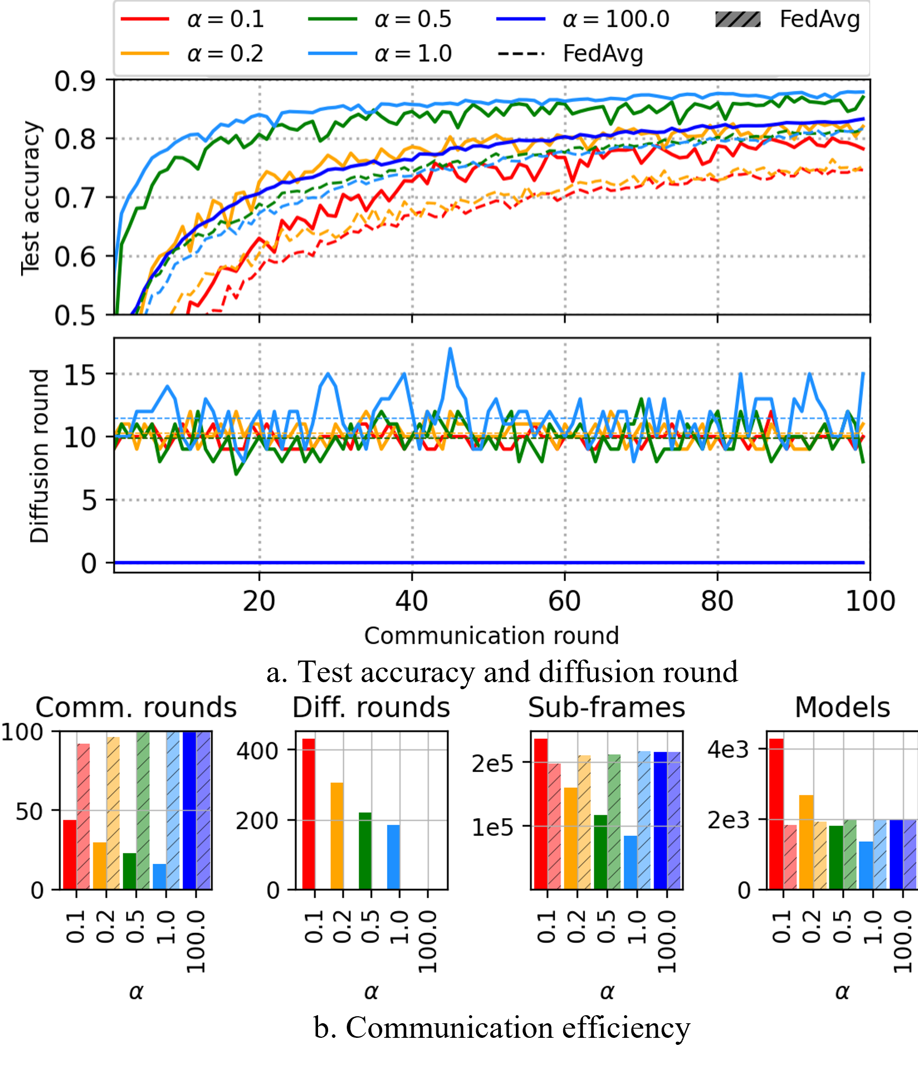
Figure 2: Performance comparison by changing concentration parameters. (Settings: $\varepsilon$ = 0.04, $\bar{\gamma}_{\textrm{min}}$ = 1.0)

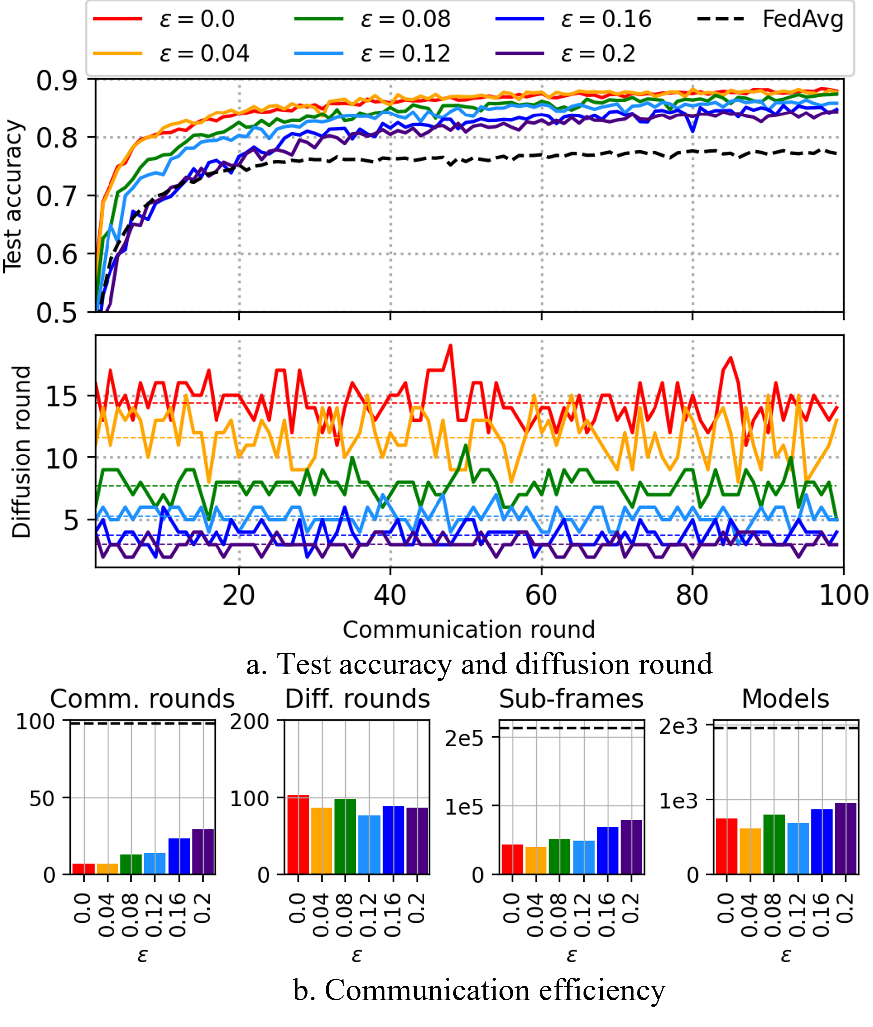
Figure 3: Performance comparison by changing minimum tolerable IID distance. (Settings: $\alpha=1.0$ $\bar{\gamma}_{\textrm{min}}=1.0$)

Figure 4: Performance comparison by changing minimum tolerable QoS. (Settings: $\alpha$ = 1.0, $\varepsilon$ = 0.04)

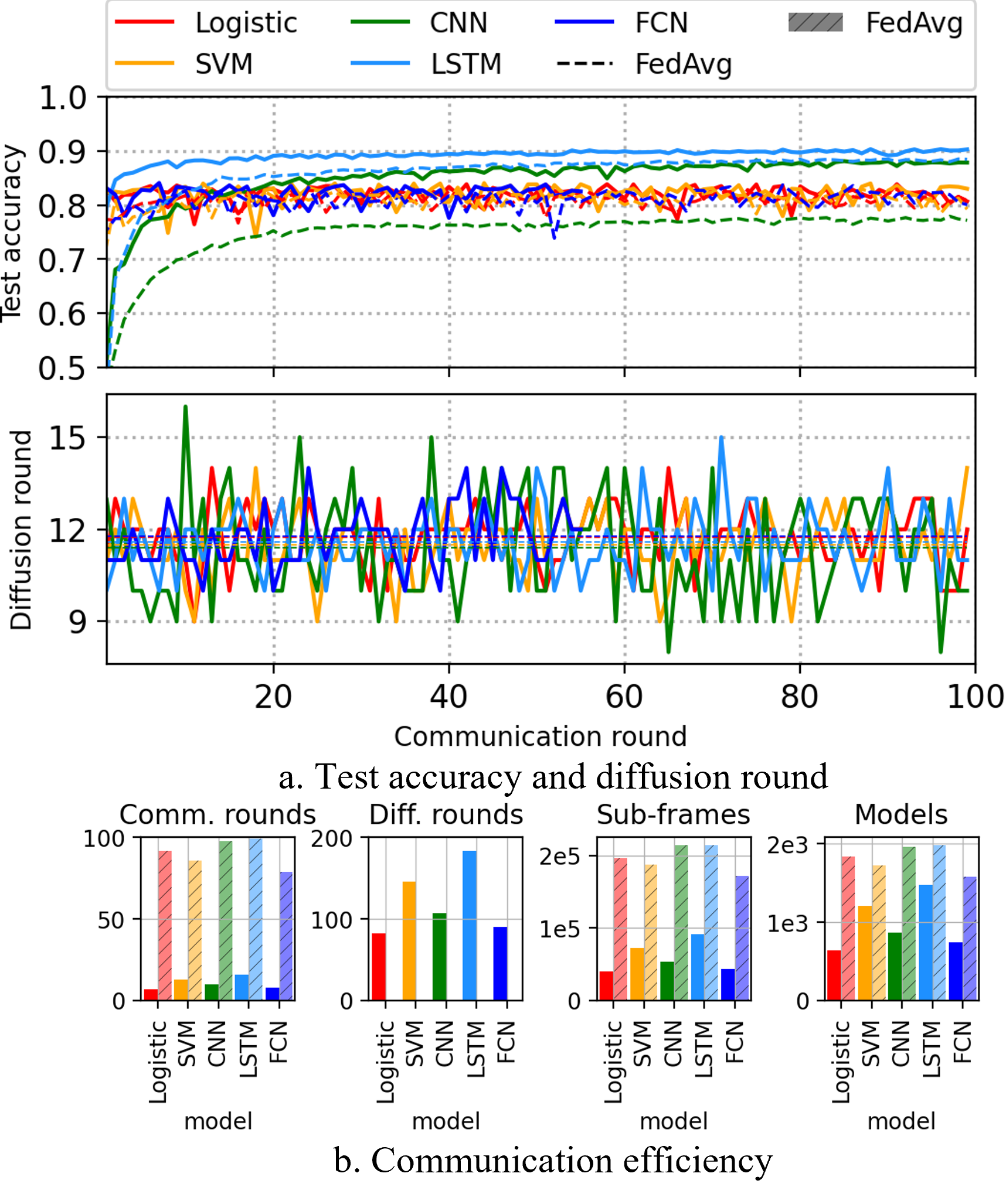
Figure 5: Performance comparison by changing ML tasks. (Settings: $\alpha$ = 1.0, $\varepsilon$ = 0.04, $\bar{\gamma}_{\textrm{min}}$ = 1.0)

VI-C Discussion on the minimum tolerable IID distance

In FedDif, BS schedules PUEs only if it can improve learning performance compared to the required bandwidth needed to diffuse the models. In other words, excessive diffusion can deteriorate the network quality and learning performance with the marginal diffusion efficiency. We define the minimum tolerable IID distance $\varepsilon$ at which the BS can determine the halting point of the diffusion. We investigate the learning performance and communication efficiency of FedDif by the various minimum tolerable IID distance, as shown in Fig. 3. We conduct several simulations with the concentration parameter and minimum tolerable QoS of 1.0, respectively, by changing $\varepsilon$. We set the target accuracy as the peak accuracy of the baseline FL, which is 77.94%. In Fig. 3(a), the dotted line represents the target accuracy of the baseline FL. We confirm that FedDif outperforms the baseline FL in every case of $\varepsilon$. Specifically, the lower $\varepsilon$ can induce more diffusion. In the case of $\varepsilon$ = 0.0, the models tend to conduct the diffusion until they train datasets of every PUE.

Fig. 3(b) shows that the number of communication rounds in the low $\varepsilon$ is the fewest while the number of consumed sub-frames and models is the largest for obtaining the target accuracy. On the other hand, the number of diffusion rounds decreases as the $\varepsilon$ becomes larger. The higher $\varepsilon$ allows only the large decrement of IID distance. Accordingly, the accuracy of lower minimum tolerable IID distance becomes higher because FedDif can approximate the DoL to uniform distribution more elaborately. The IID distance in the $\varepsilon$ = 0.2 may not be sufficiently reduced since each model can easily reach the minimum tolerable IID distance. In addition, the high value of $\varepsilon$ may deteriorate communication efficiency. We can see that the tendency for the number of consumed sub-frames and transmitted models increases by employing the higher minimum tolerable IID distance. In the high value of minimum tolerable IID distance, The model cannot sufficiently learn other users’ datasets before the global aggregation because the knowledge of the models for the PUEs’ dataset is insufficient to obtain the same effect of learning the IID dataset. Therefore, we can obtain some insights that employing the small value of $\varepsilon$ is efficient on both sides of learning performance and communication efficiency. We set the baseline $\varepsilon$ as 0.04 because it shows reasonable communication resources to achieve the required learning performance.

VI-D Discussion on the minimum tolerable QoS

In urban wireless networks, unscheduled PUEs can exist when there are no neighboring PUEs nearby or poor channel conditions to the neighboring PUEs (Isolation). Isolation may prolong the diffusion times of PUEs because PUEs continuously wait for scheduling until the required performance is achieved. We investigate the performance of FedDif by changing the minimum tolerable QoS $\bar{\gamma}_{\textrm{min}}$ that can adjust the coverage of D2D communications. Isolation may be deepened by increasing the minimum tolerable QoS. Isolation in the large minimum tolerable IID distance and QoS may deteriorate the learning performance because the less-trained models induce the aggregate of the imbalanced knowledge on the entire trained datasets in the global aggregation step. Otherwise, excessive diffusion may be performed because a few non-isolated models try to train the dataset for every PUE. Moreover, excessive diffusion requires tremendous communication resources. We investigate the performance of FedDif by building the environment where the isolation issue occurs, as shown in Fig. 4. We set the concentration parameter and minimum tolerable diffusion efficiency as 1.0 and 0.04, respectively. We also set the target accuracy as the peak accuracy of the baseline FL in the $\varepsilon$ experiment.

In Fig. 4(a), FedDif outperforms the baseline FL for every case of $\bar{\gamma}_{\textrm{min}}$. Moreover, we confirm that FedDif shows the same learning performance for every case of the different $\bar{\gamma}_{\textrm{min}}$. However, the models require more diffusion rounds when the coverage of D2D communication narrows ($\bar{\gamma}_{\textrm{min}}$ = 4.0). Specifically, the models require more diffusion rounds for the model transmission to obtain the target accuracy according to the increase of $\bar{\gamma}_{\textrm{min}}$, as shown in Fig. 4(b). Rather, in the case of higher $\bar{\gamma}_{\textrm{min}}$, the signals are less attenuated because of PUEs’ narrow coverage, which leads to a decrease in the required sub-frames. However, the opportunity for finding neighboring PUEs may decrease. In other words, the decreased opportunity may increase the number of model transmissions to achieve the required decrement in IID distance. We set the baseline $\bar{\gamma}_{\textrm{min}}$ as 1.0, which indicates the spectral efficiency in the modulation order of QPSK, to evaluate the performance of FedDif.

VI-E Empirical evaluations of FedDif

To show the efficiency of our proposed method, we measure the test accuracy, the number of diffusion rounds, and the communication efficiency metrics with commonly used ML models and datasets. In Fig. 5, we investigate the learning performance and communication costs of FedDif and the baseline FL for the various ML tasks. The ML tasks comprise Logistic, SVM, FCN, LSTM with FMNIST, and CNN with CIFAR10. For simplicity, we will call the ML tasks the model’s name, for example, CNN with CIFAR10 to CNN. We set the concentration parameter, minimum tolerable IID distance, and minimum tolerable QoS as 1.0, 0.04, and 1.0, respectively. We also set the target accuracy as the peak accuracy of the baseline FL for each task, i.e., 83.87%, 83.70%, 83.74%, 88.54%, and 77.94%, where Logistic, SVM, FCN, LSTM, and CNN, respectively.

In Fig. 5(a), the dotted line represents the accuracy of the baseline FL for each task. In CNN and LSTM, FedDif outperforms the baseline FL. Other cases, such as Logistic, SVM, and FCN, show similar performance, but the communication costs of FedAvg are higher than FedDif, as shown in Fig. 5(b). Specifically, we can see that the models converge rapidly in Logistic, SVM, FCN, LSTM, and CNN orders, resulting from the complexity of each dataset as widely known in the ML literature. Moreover, in Fig. 5(b), FedDif outperforms the baseline FedAvg in the communication costs of every task. This is because FedDif can find suitable PUEs for each model to converge the model rapidly.

In Table I, we compare the test accuracy of FedDif against the previous FL methods after 100 communication rounds. For a fair comparison, we adopt the baselines of each study as CNN with CIFAR10, FCN with MNIST, and LSTM with FMNIST. As shown in Table I, FedDif has nearly the same or exceeds test accuracy as the previous methods. FedDif shows an improved performance than TT-HF [21], at least 16.64% in FCN and up to 42.41% in CNN. Compared to STC [36], FedDif achieves better test accuracy at the minimum of 0.15% in LSTM and the maximum of 7.53% in CNN. However, several ML tasks of FedSwap [20] tend to show slightly better performance than FedDif. We can see that FedSwap is the same as the full diffusion of FedDif.

TABLE I: Comparison of the peak test accuracy.
(The number of communication rounds = 100)

ML tasks	Baseline	Previous methods			FedDif
	FedAvg	TT-HF	STC	FedSwap
CNN/CIFAR10	77.94%	45.50%	80.38%	88.99%	87.91%
FCN/MNIST	83.74%	75.54%	90.58%	92.38%	92.18%
LSTM/FMNIST	88.54%	48.84%	89.09%	90.01%	89.24%

We compare the communication costs with the previous methods for the case of CNN with CIFAR10, as shown in Table II. We measure the communication costs until achieving the test accuracy of 80%. TT-HF is not available to compare communication efficiency because it cannot achieve the target accuracy by 100 communication rounds. We can see that FedDif reduces the number of consumed sub-frames by 28.56% compared to FedSwap and 2.85 folds compared to the baseline FL. Similarly, FedDif reduces the number of transmitted models by 42.67% compared to FedSwap and 2.67 folds compared to baseline FL. However, FedDif reduces the number of transmitted models by 3.03 folds compared to STC but consumes sub-frames by 10.82 folds more than STC. The reason is that STC transmits the compressed models, but STC does not consider the channel states in wireless networks. Note that STC can be utilized as an add-on for the FedDif. Meanwhile, FedSwap requires more sub-frames relatively because of the number of model transmissions as much as the full-diffusion in FedDif. In contrast, FedDif performs diffusion rounds by optimizing the decrement of diffusion efficiency so that it requires fewer sub-frames compared to the other methods. FedDif transmits fewer models per sub-frame because only part of PUEs send their models where the IID distance decreases. Consequently, FedDif is communication-efficient because it can achieve the target accuracy despite fewer sub-frames and models.

VII Conclusion and future works

We proposed a novel diffusion strategy for preventing performance degradation by non-IID data in federated learning. We designed FedDif for the models to obtain knowledge of various local datasets before global aggregation. We regarded every user as non-IID batch data, and models can learn different non-IID data by passing through multiple users before the global aggregation step. Every model can obtain the same effect to be trained by the nearly IID dataset. Furthermore, based on auction theory, we empower communication efficiency in FedDif for the trade-off between improving learning performance and minimizing communication costs. Our study provides several research opportunities to study future works. For example, FedDif deals with the horizontal FL where the feature set of every dataset is the same. Considering vertical federated learning in which each user has a different feature set, the server aggregates the feature set is a crucial topic to tackle in future works.

TABLE II: Comparison of communication efficiency.
(Target test accuracy = 80%, Maximum communication rounds = 100)

Metrics	Baseline	Previous methods			FedDif
	FedAvg	TT-HF	STC	FedSwap
# of sub-frames	175,554	N/A	5,685	61,562	47,886
# of models	1,600	N/A	1,820	856	600

Seyoung Ahn received the B.E. degree in Computer Science and Engineering from Hanyang University, South Korea, in 2018. He is currently pursuing the M.S.-leading-to-Ph.D. degree in Computer Science and Engineering, Hanyang University, South Korea. Since 2018, he has been with the Computer Science and Engineering, Hanyang University of Engineering, South Korea. His research interests include Network optimization based on machine learning, cell-free massive MIMO, and federated learning.

Soohyeong Kim received the B.E. degree in Computer Science and Engineering from Hanyang University, South Korea, in 2019. He is currently pursuing the M.S.-leading-to-Ph.D. degree in Computer Science and Engineering at Hanyang University, South Korea. Since 2019, he has been with the Computer Science and Engineering, South Korea. His research interests include wireless mobile communication and cell-free massive MIMO networks.

Yongseok Kwon received the B.E. degree in Computer Science and Engineering from Hanyang University, South Korea, in 2019. He is currently pursuing the M.S.-leading-to-Ph.D. degree in Computer Science and Engineering at Hanyang University, South Korea. Since 2019, he has been with the Computer Science and Engineering, Hanyang University of Engineering, South Korea. His research interests include AI security, applied cryptography, and information security and privacy.

Joohan Park received the B.E. degree in Computer Science and Engineering from Hanyang University, South Korea, in 2017. He is currently pursuing the M.S.-leading-to-Ph.D. degree in Computer Science and Engineering, Hanyang University, South Korea. Since 2017, he has been with the Computer Science and Engineering, Hanyang University of Engineering, South Korea. His research interests include resource allocation by mobile base station, space-air-ground integrated network, massive IoT.

Jiseung Youn received the B.E. degree in Computer Science and Engineering from Chungnam University, South Korea, in 2020. He is currently pursuing the M.S.-leading-to-Ph.D. degree in Computer Science and Engineering at Hanyang University, South Korea. Since 2020, he has been with the Computer Science and Engineering, Hanyang University of Engineering, South Korea. His research interests include Next-Generation Cellular Communications (6G) and Internet of Things (IoT).

Sunghyun Cho received his B.S., M.S., and Ph.D. in Computer Science and Engineering from Hanyang University, Korea, in 1995, 1997, and 2001, respectively. From 2001 to 2006, he was with Samsung Advanced Institute of Technology, and with Telecommunication R&D Center of Samsung Electronics, where he has been engaged in the design and standardization of MAC and network layers of WiBro/WiMAX and 4G-LTE systems. From 2006 to 2008, he was a Postdoctoral Visiting Scholar in the Department of Electrical Engineering, Stanford University. He is currently a Professor in the dept. of Computer Science and Engineering, Hanyang University. His primary research interests are beyond 5G communications, software defined networks, and deep learning for communication systems. He is a member of the board of directors of the Institute of Electronics and Information Engineers (IEIE) and the Korean Institute of Communication Sciences (KICS).

Appendix A Implementations of FedDif

A-A Minimum tolerable QoS

Although the auction can ensure communication-efficient diffusion, the BS may conduct the full diffusion until the improvement of IID distance converges to zero. Note that the full diffusion is to participate all PUEs in the diffusion. In full diffusion, PUEs devouring substantial communication resources may exist because faraway PUEs can be paired to get any improvement of IID distance. We set the minimum tolerable QoS requirement to constraint consuming the excessive communication resources expressed as (16e). However, the isolation problem may occur when no neighboring PUE satisfies the minimum tolerable QoS. The models of the isolated PUEs may break the synchronization of FL or create an undertrained global model. This occurs in a similar issue to the insufficient batch data in centralized learning. Therefore, the higher value of the minimum tolerable QoS may deepen the isolation problem. In terms of consistency of the D2D communications, considering outage probability for PUE pairing is crucial. We pair two PUEs $i$ and $j$ by considering the outage probability as follows:

$$P_{\textrm{out}}\left(\gamma_{i,j}^{(k)}\leq\gamma_{\textrm{min}}\right)=1-\textrm{exp}\Bigg{(}\frac{-\Big{(}2^{R_{i,j}^{(k)}}-1\Big{)}}{\textrm{SNR}_{i,j}^{(k)}}\Bigg{)},$$ (A.1)

where $R_{i,j}^{(k)}=B_{k}^{(m)}\gamma_{i,j}^{(k)}$ and $\textrm{SNR}_{i,j}^{(k)}=\frac{|g_{i,j}^{(k)}|^{2}p_{i}^{(k)}}{\sigma^{2}}$ hold [21]. In FedDif, the BS only schedules PUEs if and only if their respective outage probability satisfies $P_{\textrm{out}}\left(\gamma_{i,j}^{(k)}\leq\gamma_{\textrm{min}}\right)\leq 5\%$ for a given minimum tolerable QoS $\gamma_{\textrm{min}}$. Note that the minimum tolerable QoS is given as a predefined spectral efficiency and can derive a data rate from it.

A-B Stop condition

Another concern is that immoderate diffusion may rather deteriorate communication efficiency, even though a sufficient number of diffusion rounds can reduce the IID distance. In other words, the decrement of IID distance may be insufficient compared to the required communication resources in case of low diffusion efficiency. The minimum tolerable IID distance $\varepsilon$ enables the BS to halt the diffusion and perform the global aggregation step. The halting condition for each model can be expressed as $W_{1}\left(\psi_{k}^{(m)},\mathcal{U}\right)\leq\varepsilon$. When the operator focuses on the learning performance, the number of diffusion rounds should increase. In other words, the BS can keep performing the diffusion by employing a low minimum tolerable IID distance. On the other hand, the BS should employ the high value of the minimum tolerable IID distance under the limited communication resources.

A-C Optimality of winner selection algorithm

The Kuhn-Munkres algorithm can obtain the optimal solution $\mathcal{R}^{*}$ by the principle as follows:

$$\sum_{e\in\mathcal{R}^{*}}c(e)\geq\sum_{e^{\prime}\in\mathcal{R}^{\prime}}c(e^{\prime}),\forall\mathcal{R}^{\prime}\subseteq\mathcal{M}\times\mathcal{N}_{P}$$ (A.2)

where $\mathcal{R}^{\prime}$ and $\mathcal{R}^{*}$ denote a subset of the feasible and optimal matching set, respectively. $e$ denotes a single edge. Therefore, the BS can configure the scheduling policy for the diffusion to every PUE by deriving the optimal PUE pairing information $\mathbf{i}_{k}^{*}=\left[\left\{i:(m,i)\in\mathcal{R}^{*}\right\}\right]$ and required communication resources $\mathbf{B}_{k}^{*}=\left[\left\{\tilde{B}^{(m)}_{i,k}:(m,i)\in\mathcal{R}^{*}\right\}\right]$ based on the result of the Kuhn-Munkres algorithm.

A-D Empirical analysis of the convergence trends for IID distance and diffusion efficiency

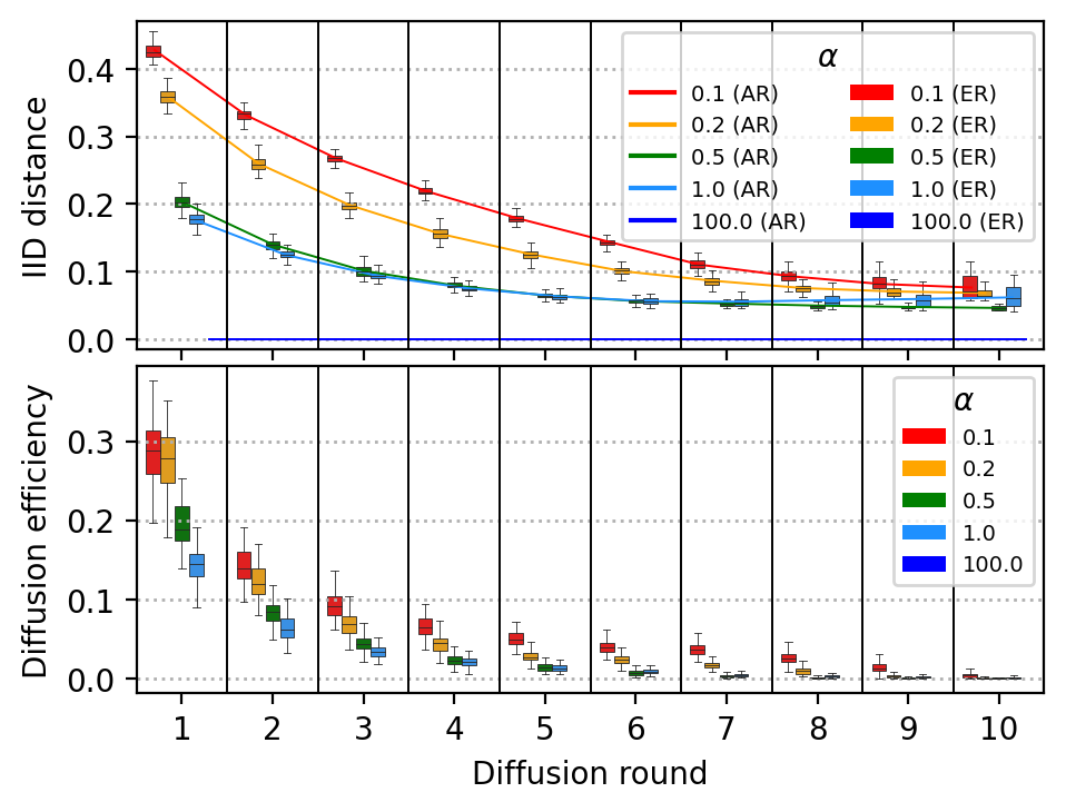
Figure 6: Convergence trends of IID distance and diffusion efficiency by different concentration parameters.

We further investigate the convergence trends of IID distance and diffusion efficiency as the diffusion rounds increase, illustrated in Fig. 6. Fig. 6 consists of two results: the analytical results (AR) and experimental results (ER) represented by line and box plots, respectively. AR of IID distance is computed utilizing the closed form of the IID distance for real-world DoL in (36). We can see that the AR and ER of IID distance converge to zero as the diffusion rounds increase. We divide the universal dataset into ten non-IID datasets by Dirichlet distribution and distribute each non-IID dataset to PUEs. We can see that the IID distances converge in ten diffusion rounds because each model can learn the entire dataset when it learns ten pieces of the universal dataset, namely, ten types of non-IID datasets. In the case of diffusion efficiency, the entire trends are the same as in the case of IID distance. The diffusion efficiency and IID distance in the case of high concentration parameter $\alpha$, which means a high degree of non-IID, steeply decrease comparing the low concentration parameter. This means that FedDif requires more diffusion rounds under a lower concentration parameter where the dataset is highly biased. Meanwhile, the diffusion mechanism entails the typical issues of existing machine learning, such as overshooting and gradient exploding. Overshooting and gradient exploding by the immoderate learning rate and upper bound of gradients may induce the weight divergence because $\eta\mu/\left|\mathcal{P}_{K}^{(m)}\right|$ can push up the upper bound of the weight difference. Gradient clipping and learning rate decay can address the overshooting and gradient exploding.

Appendix B Proof of Lemma 1

To obtain the optimal solution of the entropy maximization problem (34a), we first define the Lagrangian function $\mathcal{L}$ on the DSI $\mathbf{d}_{i_{k}^{m}}$, which can be expressed as

$$\mathcal{L}(\mathbf{d}_{i_{k}^{(m)}}[c],u)$$ (B.1)

$$=\sum_{c=1}^{C}\frac{1}{D_{\left(\mathcal{P}_{k}^{(m)}\right)}}\sum_{j\in\mathcal{P}_{k}^{(m)}}D_{j}\mathbf{d}_{j}[c]\ln\Bigg{(}\frac{1}{D_{\left(\mathcal{P}_{k}^{(m)}\right)}}\sum_{j\in\mathcal{P}_{k}^{(m)}}D_{j}\mathbf{d}_{j}[c]\Bigg{)}$$

$$\quad+u\Bigg{(}\sum_{c=1}^{C}\mathbf{d}_{i_{k}^{(m)}}[c]-1\Bigg{)}$$

where $u$ denotes the Lagrangian multiplier corresponding to the constraint (34b). The first and second order derivatives of the Lagrangian function $\mathcal{L}(\mathbf{d}_{i_{k}^{(m)}}[c],u)$ can be respectively given by

$$\frac{\partial\mathcal{L}(\mathbf{d}_{i_{k}^{(m)}}[c],u)}{\partial\mathbf{d}_{i_{k}^{(m)}}[c]}$$ (B.2)

$$=\frac{D_{i_{k}^{(m)}}}{D_{(\mathcal{P}_{k}^{(m)})}}\ln\Bigg{(}\frac{1}{D_{(\mathcal{P}_{k}^{(m)})}}\sum_{j\in\mathcal{P}_{k}^{(m)}}D_{j}\mathbf{d}_{j}[c]\Bigg{)}+\frac{D_{i_{k}^{(m)}}}{D_{(\mathcal{P}_{k}^{(m)})}}+u$$

and

$$\frac{\partial^{2}\mathcal{L}(\mathbf{d}_{i_{k}^{(m)}}[c],u)}{\partial\mathbf{d}_{i_{k}^{(m)}}^{2}[c]}=\frac{D_{i_{k}^{(m)}}^{2}}{\sum_{j\in\mathcal{P}_{k}^{(m)}}D_{j}\mathbf{d}_{j}[c]}\geq 0$$ (B.3)

From the second derivative (B.3), we can see that the Lagrangian function (B.1) is a convex function. Based on the Karush-Kuhn-Tucker (KKT) conditions, we can find the optimal solution of the Lagrangian function (B.1) as follows:

$$\frac{\partial\mathcal{L}(\mathbf{d}_{i_{k}^{(m)}}[c],u)}{\partial\mathbf{d}_{i_{k}^{(m)}}[c]}=0,$$ (B.4a)

$$u\Bigg{(}\sum_{c=1}^{C}\mathbf{d}_{i_{k}^{(m)}}[c]-1\Bigg{)}=0,$$ (B.4b)

$$u\geq 0.$$ (B.4c)

where (B.4a), (B.4b), and (B.4c) denote the stationary, complementary slackness, and dual feasibility conditions, respectively. Plugging the first derivative (B.2) into (B.4a), we can find the optimal DSI $\mathbf{d}_{i_{k}^{(m)}}^{*}$ as

$$\frac{D_{i_{k}^{(m)}}}{D_{\left(\mathcal{P}_{k}^{(m)}\right)}}\ln\Bigg{(}\frac{1}{D_{(\mathcal{P}_{k}^{(m)})}}\sum_{j\in\mathcal{P}_{k}^{(m)}}D_{j}\mathbf{d}_{j}^{*}[c]\Bigg{)}+\frac{D_{i_{k}^{(m)}}}{D_{\left(\mathcal{P}_{k}^{(m)}\right)}}+u=0$$ (B.5)

Rearranging (B.5), we can have

$$\sum_{j\in\mathcal{P}_{k}^{(m)}}D_{j}\mathbf{d}_{j}^{*}[c]=e^{-\left(\frac{D_{\left(\mathcal{P}_{k}^{(m)}\right)}}{D_{i_{k}^{(m)}}}u-\ln D_{\left(\mathcal{P}_{k}^{(m)}\right)}+1\right)}.$$ (B.6)

From the definition of the data size of the diffusion subchain $D_{(\mathcal{P}^{(m)}_{K_{t}})}=\sum_{i\in\mathcal{P}^{(m)}_{K_{t}}}D_{i}$, we can separate the left side of the equation (B.6) as

$$\sum_{j\in\mathcal{P}_{k}^{(m)}}D_{j}\mathbf{d}_{j}[c]=\sum_{j\in\mathcal{P}_{k-1}^{(m)}}D_{j}\mathbf{d}_{j}[c]+D_{i_{k}^{(m)}}\mathbf{d}_{i_{k}^{(m)}}[c]$$ (B.7)

Based on the equation (B.7), we can rewrite (B.6) as follows:

$$\mathbf{d}_{i_{k}^{(m)}}^{*}[c]$$ (B.8)

$$=\frac{1}{D_{i_{k}^{(m)}}}\Bigg{(}e^{-\left(\frac{D_{\left(\mathcal{P}_{k}^{(m)}\right)}}{D_{i_{k}^{(m)}}}u-\ln D_{\left(\mathcal{P}_{k}^{(m)}\right)}+1\right)}-\sum_{j\in\mathcal{P}_{k-1}^{(m)}}D_{j}\mathbf{d}_{j}^{*}[c]\Bigg{)}.$$

Here, we should determine the optimal Lagrangian multiplier $u^{*}$ by the complementary slackness condition (B.4b) as follows:

$$\sum_{c=1}^{C}\frac{1}{D_{i_{k}^{(m)}}}\Bigg{(}e^{-\left(\frac{D_{\left(\mathcal{P}_{k}^{(m)}\right)}}{D_{i_{k}^{(m)}}}u^{*}-\ln D_{\left(\mathcal{P}_{k}^{(m)}\right)}+1\right)}-\sum_{j\in\mathcal{P}_{k-1}^{(m)}}D_{j}\mathbf{d}_{j}^{*}[c]\Bigg{)}=1.$$ (B.9)

Based on the definition of the data size of the diffusion subchain, we can rearrange the equation (B.9) as

$$Ce^{-\left(\frac{D_{\left(\mathcal{P}_{k}^{(m)}\right)}}{D_{i_{k}^{(m)}}}u^{*}-\ln D_{\left(\mathcal{P}_{k}^{(m)}\right)}+1\right)} =D_{\left(\mathcal{P}_{k-1}^{(m)}\right)}+D_{i_{k}^{(m)}}$$ (B.10)

$$=D_{\left(\mathcal{P}_{k}^{(m)}\right)},$$

where the total data size of the diffusion subchain $\mathcal{P}_{k-1}^{(m)}$ is defined by $D_{\left(\mathcal{P}_{k-1}^{(m)}\right)}=\sum_{c=1}^{C}\sum_{j\in\mathcal{P}_{k-1}^{(m)}}D_{j}\mathbf{d}_{j}[c]$. Based on (B.10), we can determine the Lagrangian multiplier $u^{*}$ as

$$u^{*}=\frac{D_{i_{k}^{(m)}}}{D_{\left(\mathcal{P}_{k}^{(m)}\right)}}\left(\ln C-1\right)$$ (B.11)

Plugging (B.11) into (B.8), we finally obtain the optimal DSI of the model $m$ in the $k$-th diffusion round as

$$\mathbf{d}_{i_{k}^{(m)}}^{*}[c]=\frac{1}{D_{i_{k}^{(m)}}}\left(\frac{D_{\left(\mathcal{P}_{k}^{(m)}\right)}}{C}-D_{\left(\mathcal{P}_{k-1}^{(m)}\right)}\psi_{k-1}^{(m)}[c]\right).$$ (B.12)

where the relationship $D_{\left(\mathcal{P}_{k-1}^{(m)}\right)}\psi_{k-1}^{(m)}[c]=\sum_{j\in\mathcal{P}_{k-1}^{(m)}}D_{j}\mathbf{d}_{j}[c]$ holds.

Furthermore, based on constraint (34b), we can obtain the lower bound of the feasible size of the dataset for PUE $i_{k}^{(m)}$ that has the optimal DSI. Suppose the data size of PUE $i_{k}^{(m)}$ satisfies $D_{i_{k}^{(m)}}\geq 0$. Then, we have the following relationship based on constraint (34b).

$$\frac{D_{\left(\mathcal{P}_{k}^{(m)}\right)}}{C}-D_{\left(\mathcal{P}_{k-1}^{(m)}\right)}\psi_{k-1}^{(m)*}[c]\geq 0.$$ (B.13)

Rearranging (B.13) in terms of the data size $D_{i_{k}^{(m)}}$, we can have

$$\frac{D_{\left(\mathcal{P}_{k-1}^{(m)}\right)}+D_{i_{k}^{(m)}}}{C}-D_{\left(\mathcal{P}_{k-1}^{(m)}\right)}\psi_{k-1}^{(m)*}[c]\geq 0$$ (B.14)

$$D_{i_{k}^{(m)}}\geq CD_{\mathcal{P}_{k-1}^{(m)}}\psi_{k-1}^{(m)}[c]-D_{\mathcal{P}_{k-1}^{(m)}}$$ (B.15)

From the inequality (B.15), we can see that for $D_{i_{k}^{(m)}}$ to be always positive for the DoL of every class, $D_{i_{k}^{(m)}}$ should be greater than the boundary value derived as the maximum value among DoL for each class. Thus, we can obtain the lower bound of the feasible data size for each PUE as the following corollary 1.

Corollary 1.

The lower bound of the feasible size of the dataset for PUE $i_{k}^{(m)}$ that has the optimal DSI is

$$D_{i_{k}^{(m)}}\geq\max_{c}\left\{CD_{\mathcal{P}_{k-1}^{(m)}}\psi_{k-1}^{(m)}[c]-D_{\mathcal{P}_{k-1}^{(m)}}\right\},$$ (B.16)

where $C$ is the number of classes.

Appendix C Proof of Lemma 2

We will find where the IID distance for real-world DoL $\psi_{k}^{(m)}$ converges as there are sufficient diffusion rounds. First of all, the IID distance for real-world DoL $\psi_{k}^{(m)}$ is denoted as follows:

$$W_{1}(\psi_{k}^{(m)},\mathcal{U}) =\left\lVert\psi_{k}^{(m)}-\frac{1}{C}\mathbf{1}\right\rVert$$ (C.1)

$$=\sqrt{\sum_{c=1}^{C}\bigg{(}\psi_{k}^{(m)}[c]-\frac{1}{C}\bigg{)}^{2}}$$

There can exist two cases in the $k$-th diffusion round. One case is where the model $m$ discovers the PUE possessing the optimal DSI. Another case is where the model $m$ does not discover the PUE possessing the optimal DSI. In other words, the model discovers the PUE possessing real-world DSI. Suppose there exists a difference, namely, a variation $\phi_{k}[c]$ for two data sizes between the PUE possessing the real-world DSI and the optimal DSI as follows:

$$\sum_{c=1}^{C}\phi_{k}[c]=D_{i_{k}^{(m)}}-D_{i_{k}^{(m)}}^{*}=D_{\left(\mathcal{P}_{k}^{(m)}\right)}-D_{\left(\mathcal{P}_{k}^{(m)}\right)}^{*},$$ (C.2)

where $D_{i_{k}^{(m)}}$ and $D_{i_{k}^{(m)}}^{*}$ denote the data size of the PUE possessing real-world DSI and the optimal DSI, respectively. $D_{i_{k}^{(m)}}$ and $D_{i_{k}^{(m)}}^{*}$ denote the total data size of the subchains, including the PUE possessing real-world and the optimal DSI, respectively. Please note that we focus on how the IID distance is derived according to the PUE participating at the $k$-th diffusion round, regardless of what data has been trained by the model until the $(k-1)$-th diffusion round. That is, the total data size of the sub chain in the $(k-1)$-th diffusion round $D_{i_{k-1}^{(m)}}$ is same. Then, we can formulate real-world DSI as follows:

$$\mathbf{d}_{i_{k}^{(m)}}[c]=\frac{1}{D_{i_{k}^{(m)}}}\Bigg{(}\frac{D_{\left(\mathcal{P}_{k}^{(m)}\right)}^{*}}{C}-D_{\left(\mathcal{P}_{k-1}^{(m)}\right)}\psi_{k-1}^{(m)}[c]+\phi_{k}[c]\Bigg{)},$$ (C.3)

where the relationship $D_{\left(\mathcal{P}_{k}^{(m)}\right)}^{*}=D_{\left(\mathcal{P}_{k-1}^{(m)}\right)}+D_{i_{k}^{(m)}}^{*}$ holds. Then, we can have the DoL of the model $m$ when the model trains real-world dataset in the $k$-th diffusion round as

$$\psi_{k}^{(m)}[c]=\frac{1}{D_{\left(\mathcal{P}_{k}^{(m)}\right)}}\Bigg{(}D_{\left(\mathcal{P}_{k-1}^{(m)}\right)}\psi_{k-1}^{(m)}[c]+D_{i_{k}^{(m)}}\mathbf{d}_{i_{k}^{(m)}}[c]\Bigg{)}.$$ (C.4)

Plugging (C.3) into (C.4), we can have

$$\psi_{k}^{(m)}[c]=\frac{1}{D_{\left(\mathcal{P}_{k}^{(m)}\right)}}\Bigg{(}\frac{D_{\left(\mathcal{P}_{k}^{(m)}\right)}^{*}}{C}+\phi_{k}[c]\Bigg{)}.$$ (C.5)

Based on (C.2), plugging (C.5) into (C.1), we derive the closed form of the IID distance for real-world DoL at the $k$-th diffusion round as follows:

$$W_{1} (\psi_{k}^{(m)},\mathcal{U})=\sqrt{\sum_{c=1}^{C}\bigg{(}\psi_{k}^{(m)}[c]-\frac{1}{C}\bigg{)}^{2}}$$ (C.6)

$$=\sqrt{\sum_{c=1}^{C}\Bigg{(}\frac{1}{D_{\left(\mathcal{P}_{k}^{(m)}\right)}}\Bigg{(}\frac{D_{\left(\mathcal{P}_{k}^{(m)}\right)}^{*}}{C}+\phi_{k}[c]\Bigg{)}-\frac{1}{C}\Bigg{)}^{2}}$$

$$=\sqrt{\sum_{c=1}^{C}\Bigg{(}\frac{D_{\left(\mathcal{P}_{k}^{(m)}\right)}^{*}-D_{\left(\mathcal{P}_{k}^{(m)}\right)}+C\phi_{k}[c]}{CD_{\left(\mathcal{P}_{k}^{(m)}\right)}}\Bigg{)}^{2}}$$

$$=\sqrt{\sum_{c=1}^{C}\Bigg{(}\frac{C\phi_{k}[c]-\sum_{c=1}^{C}\phi_{k}[c]}{CD_{\left(\mathcal{P}_{k}^{(m)}\right)}}\Bigg{)}^{2}}$$

$$=\frac{1}{D_{\left(\mathcal{P}_{k}^{(m)}\right)}}\sqrt{\sum_{c=1}^{C}\bigg{(}\phi_{k}[c]-\frac{1}{C}\sum_{c=1}^{C}\phi_{k}[c]\bigg{)}^{2}}$$

$$=\frac{1}{D_{\left(\mathcal{P}_{k}^{(m)}\right)}}\left\lVert\phi_{k}-\bar{\phi_{k}}\right\rVert,$$

where $\phi_{k}=\{\phi_{k}[1],...,\phi_{k}[C]\}\in\mathbb{R}^{C}$ denotes the variation vector. The average variation is denoted as $\bar{\phi_{k}}=\frac{1}{C}\sum_{c=1}^{C}\phi_{k}[c]$. Here, the total data size of the diffusion chain $D_{\left(\mathcal{P}_{k}^{(m)}\right)}$ is linearly increasing as the diffusion rounds increased. However, the variation of the variation $\left\lVert\phi_{k}-\bar{\phi_{k}}\right\rVert$ is a constant value with i.i.d. for the different diffusion rounds. Therefore, we can see that the IID distance for real-world DoL $\psi_{k}^{(m)}$ asymptotically converges to zero as follows:

$$\lim_{k\to\infty}W_{1}(\psi_{k}^{(m)},\mathcal{U})=\lim_{k\to\infty}\frac{\left\lVert\phi_{k}-\bar{\phi_{k}}\right\rVert}{D_{\left(\mathcal{P}_{k}^{(m)}\right)}}=0.$$ (C.7)

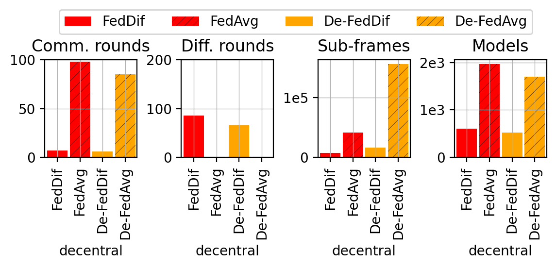
Figure 7: Comparison of (a) test accuracy, diffusion rounds, and (b) communication efficiency of fully-decentralized FedDif. Settings: $\alpha$ = 1.0, $\varepsilon$ = 0.04, $\bar{\gamma}_{\textrm{min}}$ = 1.0.

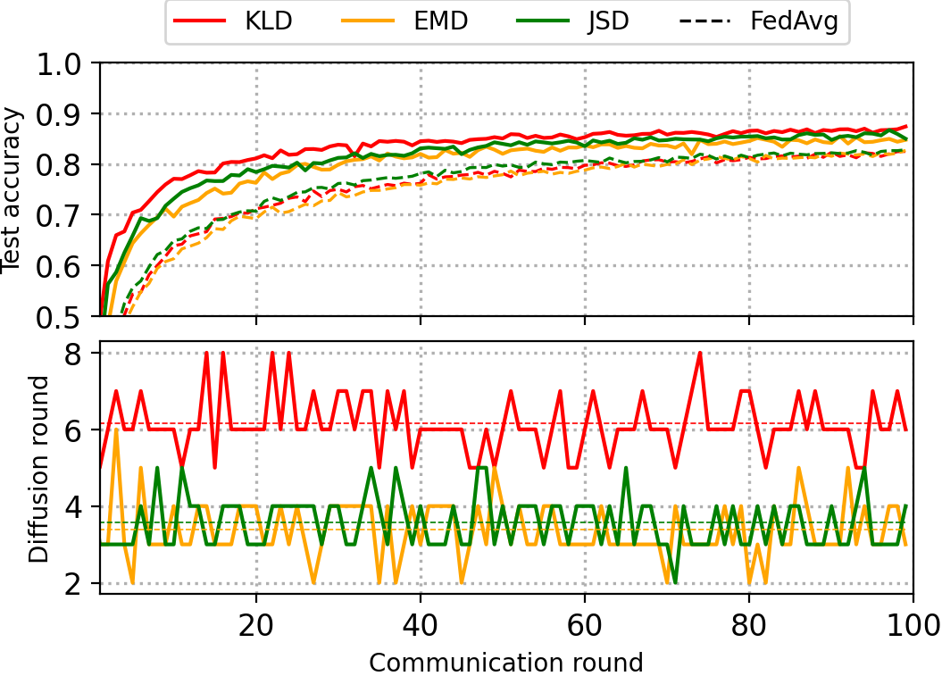
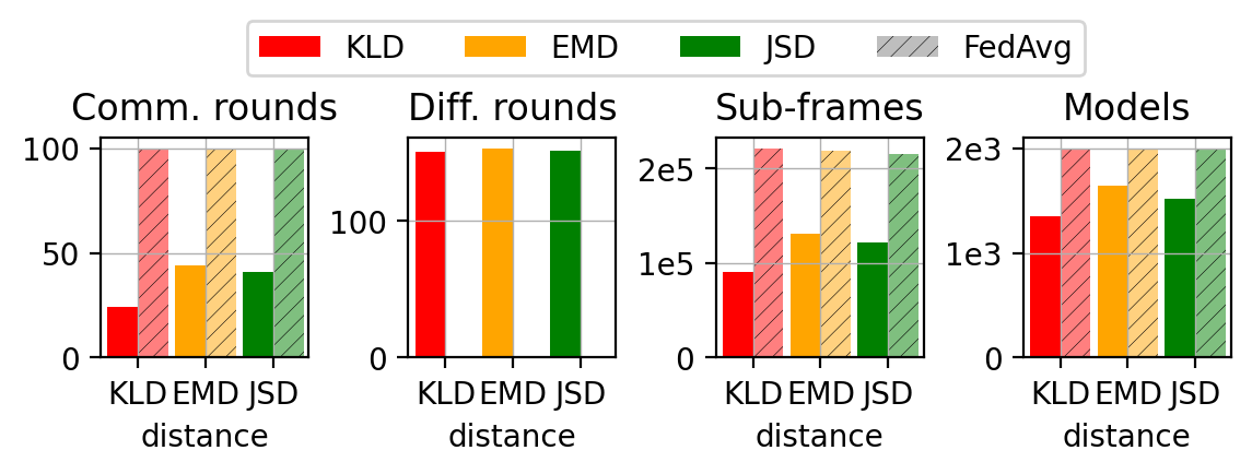
Figure 8: Comparison of (a) test accuracy, diffusion rounds, and (b) communication efficiency by changing probability distances. Settings: $\alpha$ = 1.0, $\varepsilon$ = 0.04, $\bar{\gamma}_{\textrm{min}}$ = 1.0.

Appendix D Additional experimental analysis

This section presents the additional experimental results mentioned in the main text. We additionally perform six experiments to demonstrate FedDif in the following scenarios:

1. Fig. 7 represents the performance of fully decentralized FedDif.

2. Fig. 8 represents the performance of FedDif with different probability distances.

3. Fig. 9 represents the performance of FedDif with Large-scale neural networks and complex dataset.

4. Fig. 10 represents the performance of re-trainable FedDif.

5. Fig. 11 represents the performance of FedDif with different weight initialization methods.

6. Fig. 12 represents the performance of FedDif based on the underlay mode of D2D communications.

All settings, such as the concentration parameter, minimum tolerable IID distance, and minimum tolerable QoS, of FedDif are the same as the main text described in Section VI-A.

D-A Scenario 1: fully decentralized FedDif

When the dedicated D2D channels exist for diffusion, FedDif can consider the fully decentralized FL. Fully decentralized FL is to remove the parameter aggregation server. Users delegate the representative to aggregate models or make a consensus to train models by in-network computing. We perform the experiments to delegate the representative and remove the role of BS. Figs. 7 describe the learning performance and communication costs in fully decentralized FedDif.

D-B Scenario 2: different probability distances

Based on the IID distance defined in Section III-B, FedDif measures how the DoL of the model is close to the IID data distribution. We basically employ Wasserstein-1 distance, but we can see that FedDif still works well, whatever other measurements can measure the similarity in Fig. 8. We perform experiments employing Kullback-Leibler divergence (KLD) and Jensen-Shannon divergence (JSD) to measure the IID distance.

D-C Scenario 3: large-scale neural networks and complex dataset

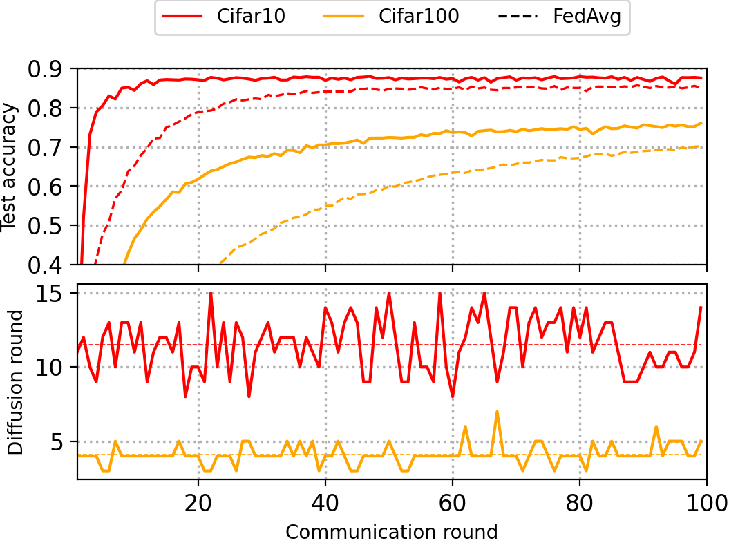
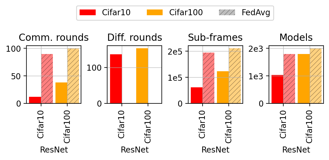
Figure 9: Comparison of (a) test accuracy, diffusion rounds, and (b) communication efficiency of FedDif with ResNet34 and CIFAR100 dataset. Settings: $\alpha$ = 1.0, $\varepsilon$ = 0.04, $\bar{\gamma}_{\textrm{min}}$ = 1.0.

In the main text, we only demonstrate FedDif using simple ML models such as SVM, logistic regression, CNN, LSTM, and FCN. However, diffusing more complex models can require more communication resources. We first investigate the performance of FedDif using the ResNet34 model, which has 600 times larger than our basic CNN model described in Fig. 9. In the case of the complex dataset, more classes may increase the complexity of the ML task because the model should distinguish samples in finer-grained scope. A finer-grained scope may confuse the model when the probabilities of multiple classes are similar to each other. To demonstrate FedDif using the complex dataset, we perform experiments using the ResNet34 model and CIFAR100. Note that the CIFAR100 dataset has ten times more classes than the CIFAR10 dataset as the following Fig. 9.

D-D Scenario 4: re-trainable FedDif

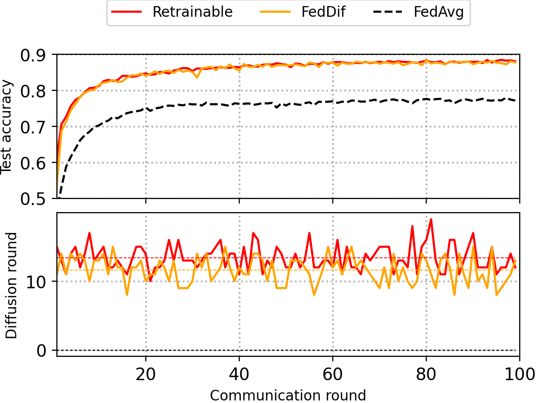
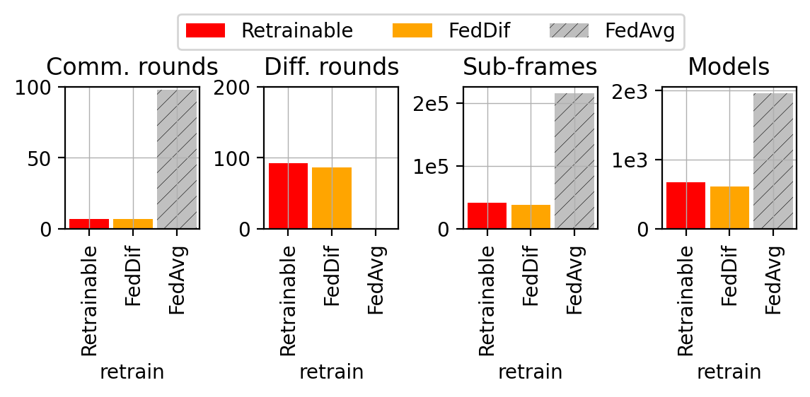
Figure 10: Comparison of (a) test accuracy, diffusion rounds, and (b) communication efficiency of re-trainable FedDif. Settings: $\alpha$ = 1.0, $\varepsilon$ = 0.04, $\bar{\gamma}_{\textrm{min}}$ = 1.0.

In FedDif, PUEs cannot re-train the previously trained model by constraint (16c). In the local training step, allowing PUEs to retrain the model can induce biased training to a specific PUE’s non-IID data by continuously learning similar non-IID data. Consequently, it may rather put the brake on the improvement of learning performance, even yield the over-fitted global model. Another concern is that retraining may occur a ping-pong problem. When there are a few neighboring PUEs in the range satisfying the minimum tolerable QoS, PUEs may continuously give and take the model for a specific PUE. The ping-pong problem may deteriorate the performance of the global model by solely learning a particular distribution of non-IID data. To demonstrate it, we conduct the additional experiments removing the constraint (16c), and the following Fig. 10 describes the performance of re-trainable FedDif.

D-E Scenario 5: different weight initialization methods

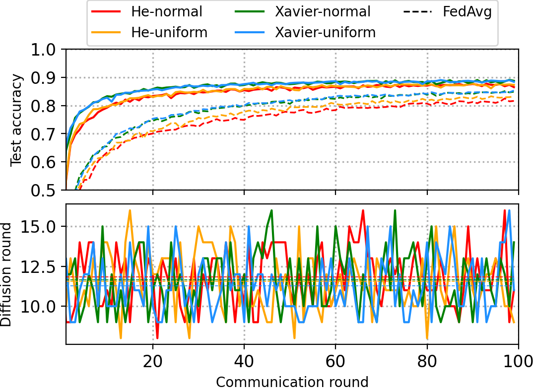
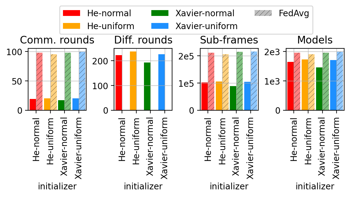
Figure 11: Comparison of (a) test accuracy, diffusion rounds, and (b) communication efficiency by changing weight initialization methods. Settings: $\alpha$ = 1.0, $\varepsilon$ = 0.04, $\bar{\gamma}_{\textrm{min}}$ = 1.0.

Weight initialization can affect the upper bound of the weight difference. Specifically, as seen in proposition 1, the weight difference by the weight initialization is determined by the weight difference between the initial weight of the global model and local models. In the model broadcasting step, if each PUE updates the parameters of the local model to the global model received from the BS without error, the effect of weight initialization can be minimized. However, different weight initialization methods can affect the internal performance of FedDif. To demonstrate it, we perform additional experiments for different weight initialization methods, as shown in Fig. (11).

D-F Scenario 6: underlay mode of D2D communications

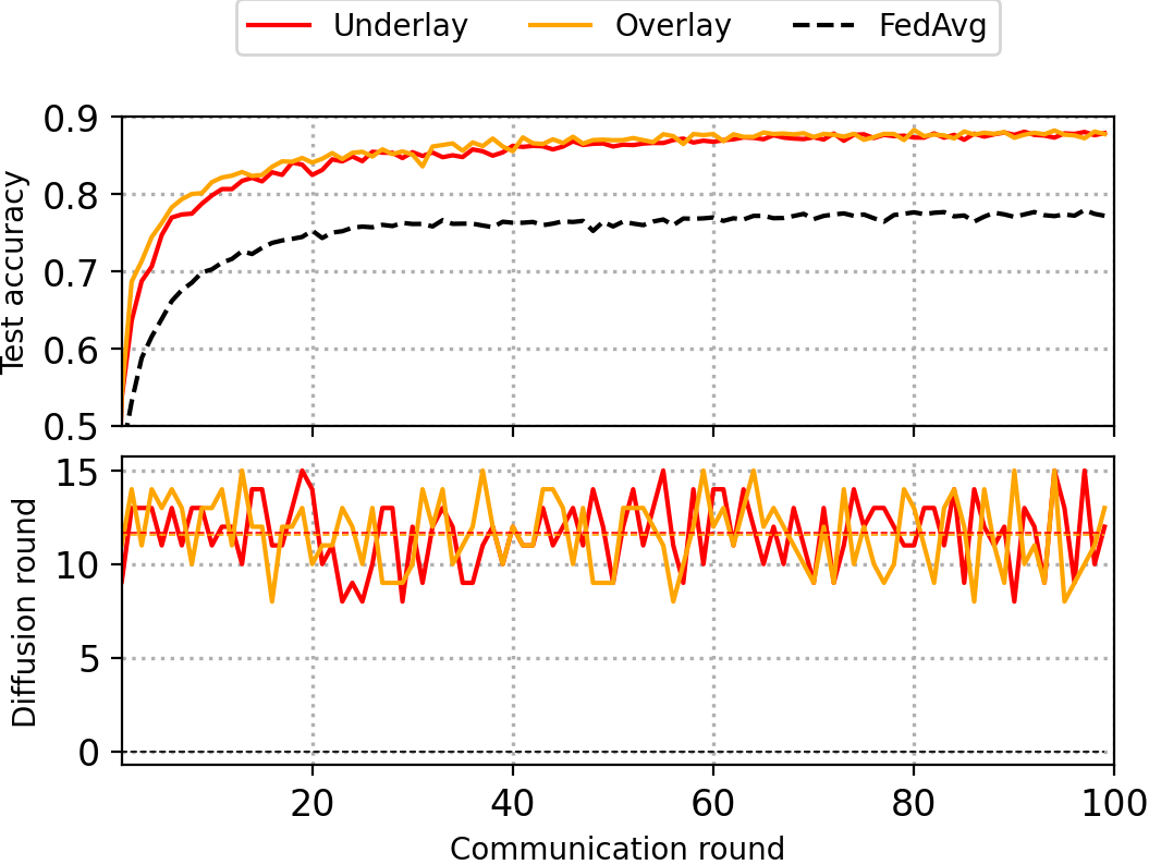
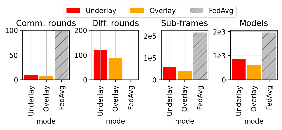
Figure 12: Comparison of (a) test accuracy, diffusion rounds, and (b) communication efficiency based on the underlay mode of D2D communications. Settings: $\alpha$ = 1.0, $\varepsilon$ = 0.04, $\bar{\gamma}_{\textrm{min}}$ = 1.0.

We perform additional experiments to consider the interference among different PUEs to investigate the communication efficiency of the underlay mode. In the additional experiments, we consider D2D communications underlying cellular networks in which each PUE only reuses the frequency resource of CUEs. Fig. 12 illustrates the performance of FedDif considering two different scenarios: the overlay and underlay mode of D2D communications. We can see that the learning performances of the two scenarios are similar, but the communication costs of the underlay mode are higher than the overlay mode. Although designing the optimal power control and resource allocation algorithms may improve the performance of FedDif utilizing the underlay mode of D2D communications, we focus on improving learning performance with non-IID data by increasing the diffusion rounds, and the resource allocation may be out of our scope.

D-G Additional investigation of the gap between the simulation and analytical results

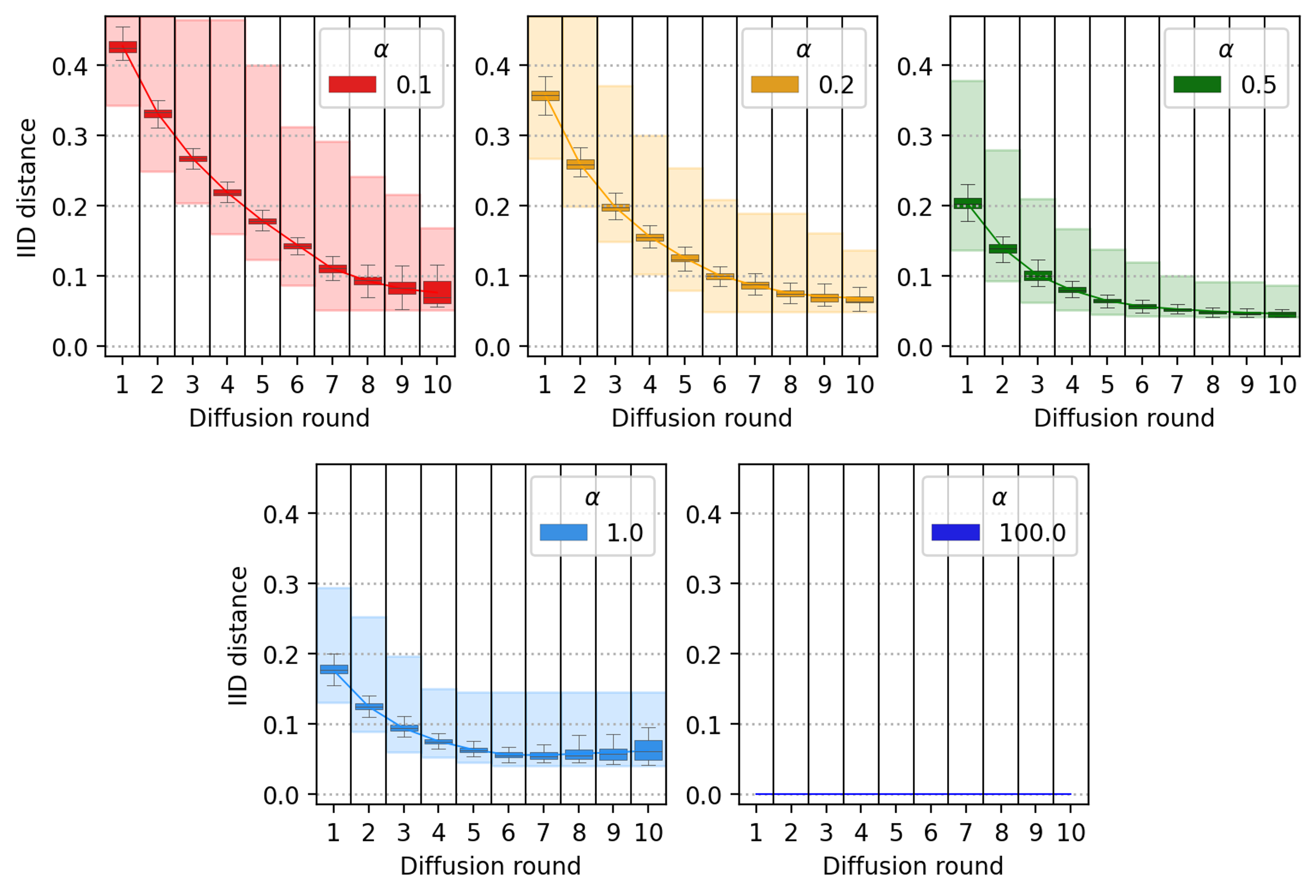
Figure 13: Convergence trends of IID distance by different concentration parameters $\alpha$. Settings: $\alpha$ = 1.0, $\varepsilon$ = 0.04, $\bar{\gamma}_{\textrm{min}}$ = 1.0.

As users have more heavily imbalanced data, the IID distance decreases steeply, starting from a higher point. This is because the more biased the model is, the faster it becomes affected by new data ever not seen before. Fig. 13 describes the convergence trends of IID distance by different concentration parameters. Note that the case of $\alpha=100.0$ is the same as the distribution of the IID dataset. Each box plot and the shading areas around box plots represent the experimental and analytical boundary of IID distance, respectively. We confirm that Lemma 2 holds, and the models do not need to diffuse in the network where every user has the IID dataset.

References

- [1] B. McMahan, E. Moore, D. Ramage, S. Hampson, and B. A. y Arcas, “Communication-efficient learning of deep networks from decentralized data,” in Proceedings of the 20th International Conference on Artificial Intelligence and Statistics, ser. Proceedings of Machine Learning Research, vol. 54, 2017, pp. 1273–1282.
- [2] E. Bagdasaryan, A. Veit, Y. Hua, D. Estrin, and V. Shmatikov, “How to backdoor federated learning,” in Proceedings of the Twenty Third International Conference on Artificial Intelligence and Statistics, ser. Proceedings of Machine Learning Research, vol. 108, 26–28 Aug 2020, pp. 2938–2948.
- [3] H. Lee, J. Kim, S. Ahn, R. Hussain, S. Cho, and J. Son, “Digestive neural networks: A novel defense strategy against inference attacks in federated learning,” Computers & Security, vol. 109, p. 102378, 2021.
- [4] K. Pillutla, S. M. Kakade, and Z. Harchaoui, “Robust aggregation for federated learning,” IEEE Transactions on Signal Processing, pp. 1–1, 2022.
- [5] H. Hsu, H. Qi, and M. Brown, “Measuring the effects of non-identical data distribution for federated visual classification,” 2019. [Online]. Available: https://arxiv.org/abs/1909.06335
- [6] Y. Zhao, M. Li, L. Lai, N. Suda, D. Civin, and V. Chandra, “Federated learning with non-iid data,” arXiv preprint arXiv:1806.00582, 2018.
- [7] Z. Zhao, C. Feng, W. Hong, J. Jiang, C. Jia, T. Q. S. Quek, and M. Peng, “Federated learning with non-iid data in wireless networks,” IEEE Transactions on Wireless Communications, pp. 1–1, 2021.
- [8] T. Li, A. K. Sahu, M. Zaheer, M. Sanjabi, A. Talwalkar, and V. Smith, “Federated optimization in heterogeneous networks,” in Proceedings of Machine Learning and Systems, I. Dhillon, D. Papailiopoulos, and V. Sze, Eds., vol. 2, 2020, pp. 429–450.
- [9] E. Jeong, S. Oh, H. Kim, J. Park, M. Bennis, and S.-L. Kim, “Communication-efficient on-device machine learning: Federated distillation and augmentation under non-iid private data,” arXiv preprint arXiv:1811.11479, 2018.
- [10] P. Kairouz, H. B. McMahan, B. Avent, A. Bellet, M. Bennis, A. N. Bhagoji, K. Bonawitz, Z. Charles, G. Cormode, R. Cummings et al., “Advances and open problems in federated learning,” Foundations and Trends® in Machine Learning, vol. 14, no. 1–2, pp. 1–210, 2021.
- [11] N. Yoshida, T. Nishio, M. Morikura, K. Yamamoto, and R. Yonetani, “Hybrid-fl for wireless networks: Cooperative learning mechanism using non-iid data,” in ICC 2020 - 2020 IEEE International Conference on Communications (ICC), 2020, pp. 1–7.
- [12] M. Luo, F. Chen, D. Hu, Y. Zhang, J. Liang, and J. Feng, “No fear of heterogeneity: Classifier calibration for federated learning with non-iid data,” Advances in Neural Information Processing Systems, vol. 34, 2021.
- [13] L. Zhang, Y. Luo, Y. Bai, B. Du, and L.-Y. Duan, “Federated learning for non-iid data via unified feature learning and optimization objective alignment,” in Proceedings of the IEEE/CVF International Conference on Computer Vision, 2021, pp. 4420–4428.
- [14] H. Wang, Z. Kaplan, D. Niu, and B. Li, “Optimizing federated learning on non-iid data with reinforcement learning,” in IEEE INFOCOM 2020 - IEEE Conference on Computer Communications, 2020, pp. 1698–1707.
- [15] C. Briggs, Z. Fan, and P. Andras, “Federated learning with hierarchical clustering of local updates to improve training on non-iid data,” in 2020 International Joint Conference on Neural Networks (IJCNN), 2020, pp. 1–9.
- [16] M. Duan, D. Liu, X. Chen, R. Liu, Y. Tan, and L. Liang, “Self-balancing federated learning with global imbalanced data in mobile systems,” IEEE Transactions on Parallel and Distributed Systems, vol. 32, no. 1, pp. 59–71, 2021.
- [17] K. Kopparapu, E. Lin, and J. Zhao, “Fedcd: Improving performance in non-iid federated learning,” arXiv preprint arXiv:2006.09637, 2020.
- [18] N. Onoszko, G. Karlsson, O. Mogren, and E. L. Zec, “Decentralized federated learning of deep neural networks on non-iid data,” arXiv preprint arXiv:2107.08517, 2021.
- [19] C. Hu, J. Jiang, and Z. Wang, “Decentralized federated learning: A segmented gossip approach,” arXiv preprint arXiv:1908.07782, 2019.
- [20] T.-C. Chiu, Y.-Y. Shih, A.-C. Pang, C.-S. Wang, W. Weng, and C.-T. Chou, “Semisupervised distributed learning with non-iid data for aiot service platform,” IEEE Internet of Things Journal, vol. 7, no. 10, pp. 9266–9277, 2020.
- [21] F. P.-C. Lin, S. Hosseinalipour, S. S. Azam, C. G. Brinton, and N. Michelusi, “Semi-decentralized federated learning with cooperative d2d local model aggregations,” IEEE Journal on Selected Areas in Communications, vol. 39, no. 12, pp. 3851–3869, 2021.
- [22] S. Savazzi, M. Nicoli, and V. Rampa, “Federated learning with cooperating devices: A consensus approach for massive iot networks,” IEEE Internet of Things Journal, vol. 7, no. 5, pp. 4641–4654, 2020.
- [23] S. Savazzi, M. Nicoli, M. Bennis, S. Kianoush, and L. Barbieri, “Opportunities of federated learning in connected, cooperative, and automated industrial systems,” IEEE Communications Magazine, vol. 59, no. 2, pp. 16–21, 2021.
- [24] X. Zhang, Y. Liu, J. Liu, A. Argyriou, and Y. Han, “D2d-assisted federated learning in mobile edge computing networks,” in 2021 IEEE Wireless Communications and Networking Conference (WCNC), 2021, pp. 1–7.
- [25] N. H. Tran, W. Bao, A. Zomaya, M. N. H. Nguyen, and C. S. Hong, “Federated learning over wireless networks: Optimization model design and analysis,” in IEEE INFOCOM 2019 - IEEE Conference on Computer Communications, 2019, pp. 1387–1395.
- [26] M. Chen, Z. Yang, W. Saad, C. Yin, H. V. Poor, and S. Cui, “A joint learning and communications framework for federated learning over wireless networks,” IEEE Transactions on Wireless Communications, vol. 20, no. 1, pp. 269–283, 2021.
- [27] J. Mills, J. Hu, and G. Min, “Communication-efficient federated learning for wireless edge intelligence in iot,” IEEE Internet of Things Journal, vol. 7, no. 7, pp. 5986–5994, 2020.
- [28] S. Ahn, S. Kim, Y. Kwon, J. Park, J. Youn, and S. Cho, “Communication-efficient diffusion strategy for performance improvement of federated learning with non-iid data,” 2022. [Online]. Available: https://arxiv.org/abs/2207.07493
- [29] D. Tse and P. Viswanath, Fundamentals of wireless communication. Cambridge university press, 2005.
- [30] M. Arjovsky, S. Chintala, and L. Bottou, “Wasserstein generative adversarial networks,” in Proceedings of the 34th International Conference on Machine Learning, ser. Proceedings of Machine Learning Research, D. Precup and Y. W. Teh, Eds., vol. 70. PMLR, 06–11 Aug 2017, pp. 214–223. [Online]. Available: https://proceedings.mlr.press/v70/arjovsky17a.html
- [31] J. Park, S. Kim, J. Youn, S. Ahn, and S. Cho, “Low-complexity data collection scheme for uav sink nodes in cellular iot networks,” IEEE Transactions on Vehicular Technology, vol. 70, no. 5, pp. 4865–4879, 2021.
- [32] T. H. T. Le, N. H. Tran, T. LeAnh, T. Z. Oo, K. Kim, S. Ren, and C. S. Hong, “Auction mechanism for dynamic bandwidth allocation in multi-tenant edge computing,” IEEE Transactions on Vehicular Technology, vol. 69, no. 12, pp. 15 162–15 176, 2020.
-
[33]
3GPP, “Study on evaluation methodology of new Vehicle-to-Everything (V2X) use
cases for LTE and NR,” 3rd Generation Partnership Project (3GPP),
Technical Report (TR) 37.885, 06 2019, version 15.3.0. [Online]. Available:
https://portal.3gpp.org/desktopmodules/Specifications
/SpecificationDetails.aspx?specificationId=3209 - [34] A. Krizhevsky, G. Hinton et al., “Learning multiple layers of features from tiny images,” 2009.
- [35] H. Xiao, K. Rasul, and R. Vollgraf. (2017) Fashion-mnist: a novel image dataset for benchmarking machine learning algorithms.
- [36] F. Sattler, S. Wiedemann, K.-R. Müller, and W. Samek, “Robust and communication-efficient federated learning from non-i.i.d. data,” IEEE Transactions on Neural Networks and Learning Systems, vol. 31, no. 9, pp. 3400–3413, 2020.