Towards two-loop automation in OpenLoops

Abstract

NLO scattering amplitudes are provided by fully automated numerical tools, such as OpenLoops, for a very wide range of processes. In order to match the numerical precision of current and future collider experiments, the higher precision of NNLO calculations is essential, and their automation in a similar tool a highly desirable goal.

In our approach, D-dimensional two-loop amplitudes are decomposed into Feynman integrals with four-dimensional numerators and (D-4)-dimensional remainders. The latter are reconstructed through process-independent rational counterterm insertions into lower-loop diagrams, while the first are expressed as loop momentum tensor integrals contracted with tensor coefficients.

In this article, we describe a completely generic algorithm, first presented in [1], for the efficient and numerically stable construction of these tensor coefficients. This algorithm is fully implemented in the OpenLoops framework for QED and QCD corrections to the Standard Model. For this implementation we present performance studies on numerical stability and CPU efficiency.

1 Introduction

Scattering amplitudes computed in perturbation theory are a key ingredient for Monte Carlo simulations of scattering processes at colliders. Tree and one-loop amplitudes, required for LO and NLO predictions, can be obtained by numerical tools, such as OpenLoops [2, 3, 4], in a fully automated way. In order to meet the precision requirements of the LHC and future colliders NNLO predictions, involving two-loop amplitudes, are essential for a wide range of processes. While dedicated NNLO calculations exist for many $2\to 2$ and a few $2\to 3$ processes, an automated NNLO tool would strongly augment the scope of NNLO phenomenology.

Scattering amplitudes at a given loop order $L$ are computed from Feynman diagrams $\Gamma$,

$$\mathcal{M}_{L}(h)\,=\,\sum\limits_{\Gamma}{\mathcal{M}}_{{L},{\Gamma}}(h){},$$ (1)

where $h$ denotes the helicity configuration of the external particles of the process at hand. For processes with $\mathcal{M}_{0}\neq 0$ the helicity and colour-summed squared tree-level amplitude

$$\mathcal{W}_{\scriptscriptstyle{\text{LO}}}\,=\,\frac{1}{N_{\rm{hcs}}}\sum\limits_{h,\mathrm{col}}|\mathcal{M}_{0}(h)|^{2}{},$$ (2)

constitutes the LO contribution of the scattering probability density. Here, $1/N_{\rm{hcs}}$ encodes the average over initial-state helicity and colour d.o.f as well as symmetry factors (see [4]). A NLO calculation consists of a real-emission contribution, which has the same form as (2) with one extra unresolved particle, and the virtual contribution computed from the Born-loop interference

$$\mathcal{W}_{\scriptscriptstyle{\text{NLO}}}^{\scriptscriptstyle{\text{virtual}}}\,=\,\frac{1}{N_{\rm{hcs}}}\sum\limits_{h,\mathrm{col}}2\,\mathrm{Re}\Big{[}\mathcal{M}_{0}^{*}(h)\mathbf{R}\bar{\mathcal{M}}_{1}(h)\Big{]},$$ (3)

where $\mathbf{R}$ denotes the renormalisation procedure and the bar an amplitude computed in $D$ dimensions.

A NNLO calculation consists of three contributions. The double-real part has the same form as (2) with two extra unresolved particles, the real-virtual part has the same form as (3) with one extra particle, and the double-virtual contribution is given by

$$\mathcal{W}_{\scriptscriptstyle{\text{NNLO}}}^{\scriptscriptstyle{\text{virtual}}}\,=\,\sum\limits_{h,\mathrm{col}}2\,\mathrm{Re}\Big{[}\mathcal{M}_{0}^{*}(h)\,\mathbf{R}\bar{\mathcal{M}}_{2}(h)\Big{]}+|\mathbf{R}\bar{\mathcal{M}}_{1}(h)|^{2}.$$ (4)

In the following, we will review the existing tree and one-loop OpenLoops program, which provides all these contributions except for the first term in (4). We will then discuss the requirements for an automated two-loop tool, and present a major building block of such a tool, namely a new algorithm for the numerical construction of two-loop integrands.

2 Tree-level and one-loop amplitude construction in OpenLoops

In OpenLoops, tree-level diagrams are constructed from subtrees $w_{a}$ through recursion steps

$$w^{\alpha}_{a}\,=\,\parbox{57.50026pt}{\includegraphics[height=28.45274pt]{diaTreeBI}}\,=\,\parbox{57.50026pt}{\includegraphics[height=56.9055pt]{diaTreeBII}}\,=\,\frac{X_{\beta\gamma}^{\alpha}(k_{b},k_{c})}{k_{a}^{2}-m_{a}^{2}}w^{\beta}_{b}w^{\gamma}_{c},$$ (5)

from two smaller subtrees, starting from the wave functions of the external particles. The kernel $X$ is derived from the Feynman rule of the connecting vertex and adjacent propagator with mass $m_{a}$ and momentum $k_{a}$. The recursion ends in connecting two subtrees into the full diagram. A high level of efficiency is achieved by recycling subtrees in multiple tree and loop diagrams.

Numerical tools construct the numerators of Feynman integrals in integer dimensions. Typically, one-loop amplitudes $\bar{\mathcal{M}}_{1}$ in $D$ dimensions are split into an amplitude $\mathcal{M}_{1}$ constructed from Feynman integrals with four-dimensional numerators and a remainder stemming from $(D-4)$-dimensional numerator parts. The latter can be reconstructed through a finite set of process-independent rational counterterms [5, 6, 7, 8], which together with the one-loop UV counterterms are inserted into all possible tree-level diagrams, resulting in the counterterm amplitude $\mathcal{M}^{\scriptscriptstyle{\text{(CT)}}}_{0,1}(h)$. The renormalised $D$-dimensional amplitude is then computed as

$$\mathbf{R}\bar{\mathcal{M}}_{1}(h)=\mathcal{M}_{1}(h)+\mathcal{M}^{\scriptscriptstyle{\text{(CT)}}}_{0,1}(h).$$ (6)

The amplitude of a one-loop diagram $\Gamma$ is given by

$$\mathcal{M}_{1,\Gamma}(h)=\vbox{\hbox{\scalebox{1.0}{\includegraphics[height=76.82243pt]{diaClosedLoop}}}}={C}_{{1},{\Gamma}}\,\int\!\mathrm{d}\bar{q}\;\frac{{\rm Tr}\left[S_{1}(q,h_{1}^{(1)})\!\cdots\!S_{N}({q,h_{N}^{(1)}})\right]}{D_{0}\!\cdots\!D_{N-1}}$$ (7)

with the colour factor ${C}_{{1},{\Gamma}}$, the integration measure in loop momentum space $\int\!\mathrm{d}\bar{q}=\mu^{2{\varepsilon}}\int\frac{\mathrm{d}^{{}^{D}}\!\bar{q}}{(2\pi)^{{}^{D}}}$ and scalar propagator denominators $D_{a}(q)=(q+p_{a})^{2}-m_{a}^{2}$ with mass $m_{a}$ and external momentum $p_{a}$. The numerator factorises into loop segments with at most linear $q$-dependence,

$$S_{a}(q,h_{a}^{(1)}) = \parbox{57.50026pt}{ \includegraphics[height=51.21495pt]{diasegmentAa}}=\{Y_{\sigma}^{a}+Z_{\nu;\sigma}^{a}\,{q^{\nu}}\}\,w^{\sigma}_{a}(h_{a}^{(1)}),$$ (8)

which consist of a loop vertex and propagator encoded in the universal building blocks $Y,Z$ and one or two external sub-trees $w_{a}$ with external momentum $k_{a}$ and helicity configuration $h_{a}^{(1)}$. Each segment is a matrix with Lorentz or spinor indices $\beta_{a-1},\beta_{a}$, and the trace in (7) connects the indices $\beta_{0}$ and $\beta_{N}$. The contribution of the diagram $\Gamma$ to (3) can be written as

$$\mathcal{W}_{01,\Gamma} = \bar{\sum\limits_{h,\mathrm{col}}}2\,\mathrm{Re}\Big{[}\mathcal{M}_{0}^{*}\mathcal{M}_{1,\Gamma}\Big{]}=\mathrm{Re}\left[\int\!\mathrm{d}\bar{q}\;\frac{\rm{Tr}\left[\mathcal{U}_{N}(q)\right]}{D_{0}\cdots D_{N-1}}\right]$$ (9)

where the integrand numerator

$$\mathcal{U}_{N}(q) = \sum\limits_{h}\mathcal{U}_{0}(h)\prod\limits_{a=1}^{N}S_{a}(q,h_{a}^{(1)})\,=\,\sum\limits_{h_{N}^{(1)}}\cdots\left(\sum\limits_{h_{1}^{(1)}}\mathcal{U}_{0}(h)S_{1}(q,h_{1}^{(1)})\right)\!\cdots\!S_{N}({q,h_{N}^{(1)}})$$ (10)

factorises into nested helicity sums of segments and the Born–colour interference term

$$\mathcal{U}_{0}(h)=2\left(\sum\limits_{\mathrm{col}}\mathcal{M}_{0}^{*}(h){C}_{{1},{\Gamma}}\right).$$ (11)

In OpenLoops, a one-loop diagram is cut-opened at a chosen loop propagator $D_{0}$ and the resulting chain of segments in (10) is constructed recursively through steps

$$\mathcal{U}_{k}(q,\check{h}_{k})\,=\,\sum\limits_{h_{k}^{(1)}}\mathcal{U}_{k-1}(q,\check{h}_{k-1})S_{k}(q,h_{k}^{(1)})$$ (12)

starting from $\mathcal{U}_{0}(h)$, and employing an on-the-fly summation of the segment helicities $h_{k}^{(1)}$, introduced in [3]. The numerator is systematically decomposed as

$$\mathcal{U}_{k}(q,\check{h}_{k})=\sum\limits_{r=0}^{k}\mathcal{U}_{k,\mu_{1}\ldots\mu_{r}}(\check{h}_{k})\,{q^{\mu_{1}}\ldots q^{\mu_{r}}},$$ (13)

and the numerical recursion is implemented at the level of the tensor coefficients $\mathcal{U}_{k,\mu_{1}\ldots\mu_{r}}$, retaining the analytical structure in $q$ throughout the amplitude construction. The tensor integrals in the resulting Born–loop interference

$$\mathcal{W}_{01,\Gamma}=\sum\limits_{r=0}^{N}\mathcal{U}_{N,\mu_{1}\ldots\mu_{r}}\int\!\mathrm{d}^{D}\!\!\bar{q}\;\frac{q^{\mu_{1}}\ldots q^{\mu_{r}}}{D_{0}\!\cdots\!D_{N-1}}$$ (14)

are either reduced a posteriori, using external libraries such as Collier [9], or using the on-the-fly reduction method [3] with Collier or OneLoop [10] for the final evaluation of scalar integrals. This completely generic algorithm is fully implemented for QCD and EW corrections to the SM and available in the public OpenLoops tool [4].

3 Two-loop amplitude construction

Following the same strategy, we decompose the numerators of two-loop integrands into a part that can be numerically constructed in four dimensions, and $(D-4)$-dimensional remainders. In [11, 12, 13] it was demonstrated that the renormalised $D$-dimensional two-loop amplitude can be split into amplitudes and counterterms computed with four-dimensional loop numerators,

$$\mathbf{R}\bar{\mathcal{M}}_{2}(h)=\mathcal{M}_{2}(h)+\mathcal{M}^{\scriptscriptstyle{\text{(CT)}}}_{1,1}(h)+\mathcal{M}^{\scriptscriptstyle{\text{(CT)}}}_{0,2}(h)+\mathcal{M}^{\scriptscriptstyle{\text{(CT)}}}_{0,1,1}(h)$$ (15)

where the four terms on the rhs are the unrenormalised two-loop amplitude, the one-loop amplitude with one-loop rational and UV counterterm insertions, the tree-level amplitude with two-loop rational and UV counterterm insertions, and the tree-level amplitude with double one-loop rational and UV counterterm insertions. The full set two-loop rational terms of UV origin were computed in [11, 12, 13] for QED and QCD corrections to the SM in a generic renormalisation scheme. Rational terms stemming from IR divergences are currently under investigation.

The calculation of the two-loop amplitude $\mathcal{M}_{2}$ interfered with the Born $\mathcal{M}_{0}$, is then split into the construction of the integrand at the level of loop momentum tensor coefficients, and the subsequent reduction and evaluation of the tensor integrals. In the following we present an algorithm for the first of these steps, focusing on the case of irreducible diagrams, which become 1PI on amputation of all external subtrees.

The amplitude of an irreducible two-loop diagram $\Gamma$ is given by

$$\mathcal{M}_{2,\Gamma}(h) = \vbox{\hbox{\scalebox{1.0}{\includegraphics[width=168.07355pt]{diaTwoLoopClosedDressing}}}}={C}_{{2},{\Gamma}}\!\int\!\!\mathrm{d}\bar{q}_{1}\!\!\int\!\mathrm{d}\bar{q}_{2}\frac{\mathcal{N}(q_{1},q_{2},h)}{\prod\limits_{i=1}^{3}\mathcal{D}^{(i)}(\bar{q}_{i})}\Big{|}_{q_{3}=-(q_{1}+q_{2})}$$ (16)

with the numerator of the integrand factorising into three chains connected by two vertices $\mathcal{V}_{0},\mathcal{V}_{1}$,

$$\mathcal{N}({q_{1}},{q_{2}},h)=\prod\limits_{i=1}^{3}\mathcal{N}^{(i)}({q_{i}},h^{(i)})\prod\limits_{j=0}^{1}\mathcal{V}_{j}({q_{1}},{q_{2}},h_{j}^{(V)}\,),$$ (17)

and the three denominator chains $(i=1,2,3)$ factorising into scalar propagator denominators,

$$\mathcal{D}^{(i)}(\bar{q}_{i}) = D^{(i)}_{0}(\bar{q}_{i})\cdots D^{(i)}_{N_{i}-1}(\bar{q}_{i})\,,\qquad\mbox{where}\quad D^{(i)}_{a}(\bar{q}_{i})\,=\,\left(\bar{q}_{i}+p_{ia}\right)^{2}-m_{ia}^{2}\,.$$ (18)

Each chain depends on a single loop momentum and further factorises into segments of the same structure as at one loop,

$$\mathcal{N}^{(i)}(q_{i},h^{(i)})=S_{0}^{(i)}({q_{i},h_{0}^{(i)}})\cdots S_{N_{i}-1}^{(i)}({q_{i}},h_{N_{i}-1}^{(i)}).$$ (19)

The helicity labels are defined in an additive way (see [1]), such that

$$h=\sum\limits_{i=1}^{3}h^{(i)}+\sum\limits_{j=0}^{1}h_{j}^{(V)},\qquad h^{(i)}=\sum\limits_{a=1}^{N_{i}-1}h_{a}^{(i)}.$$ (20)

To compute the contribution of this diagram to (4), its colour factor ${C}_{{2},{\Gamma}}$ is interfered with the Born,

$$\mathcal{U}_{0}(h)=2\,\sum_{\mathrm{col}}\mathcal{M}^{*}_{0}(h)\,{C}_{{2},{\Gamma}},$$ (21)

to form a building block in the construction of the numerator of the Born two-loop interference,

$$\mathcal{U}({q_{1}},{q_{2}})=\sum\limits_{h}\mathcal{U}_{0}({h})\,\mathcal{N}({q_{1}},{q_{2}},{h})=\sum_{r_{1}=0}^{R_{1}}\sum_{r_{2}=0}^{R_{2}}{\mathcal{U}}_{\mu_{1}\cdots\mu_{r_{1}}\nu_{1}\cdots\nu_{r_{2}}}q_{1}^{\mu_{1}}\cdots q_{1}^{\mu_{r_{1}}}\,q_{2}^{\nu_{1}}\cdots q_{2}^{\nu_{r_{2}}}.$$ (22)

This construction is again performed at the level of the loop momentum tensor coefficients. The most efficient recursive algorithm was found through a cost analysis of possible candidates for a wide range of processes [1]. This completely generic algorithm is fully implemented and validated for QED and QCD corrections to SM processes. It consists of the following steps:

0.

The chains are sorted by length, such that $N_{1}\geq N_{2}\geq N_{3}$. The order of $\mathcal{V}_{0}$ and $\mathcal{V}_{1}$ is determined by vertex type, in a way that the efficiency of the subsequent steps is maximised (see [1] for details).

1.

The shortest chain is constructed through the recursion ($n=0,\ldots,N_{3}-1$)

$$\mathcal{N}^{(3)}_{n}({q_{3}},{\hat{h}_{n}^{(3)}})=\mathcal{N}^{(3)}_{n-1}({q_{3}},{\hat{h}_{n-1}^{(3)}})\cdot S_{n}^{(3)}({q_{3}},{h_{n}^{(3)}})\quad\text{with}\quad\hat{h}_{n}^{(3)}=\sum\limits_{a=1}^{n}h_{a}^{(3)},$$ (23)

recycling intermediate results in multiple Feynman diagrams.

2.

The full diagram interfered with the Born is then constructed through a sequence of recursions starting from $\mathcal{U}^{(1)}_{-1}(h)=\mathcal{U}_{0}(h)$ defined in (21):

• The longest chain, which usually contains the majority of helicity d.o.f., is constructed as

  $$\mathcal{U}^{(1)}_{n}({q_{1}},{\check{h}_{n}^{(1)}})={\sum\limits_{h_{n}^{(1)}}}\mathcal{U}^{(1)}_{n-1}({q_{1}},{\check{h}_{n-1}^{(1)}})\cdot S_{n}^{(1)}({q_{1}},{h_{n}^{(1)}})\quad\text{with}\quad{\check{h}_{n}^{(1)}=h-\sum\limits_{a=1}^{n}h_{a}^{(1)}}$$ (24)

  and $n=0,\ldots,N_{1}-1$. The on-the-fly summation of a large fraction of the helicity configurations at a stage where the intermediate results depend on a single loop momentum $q_{1}$ is an important reason for the efficiency of the algorithm.

• The vertex $\mathcal{V}_{1}$ is connected,

  $${\mathcal{U}_{1}^{(13)}}({q_{1}},{q_{3}},{h^{(2)}+h_{0}^{(V)}})={\sum\limits_{h^{(3)},h_{1}^{(V)}}}\;\mathcal{U}^{(1)}_{N_{1}-1}({q_{1}},{h-h^{(1)}})\;\mathcal{N}^{(3)}_{N_{3}-1}({q_{3}},{h^{(3)}})\;\mathcal{V}_{1}({q_{1}},{q_{3}},h_{1}^{(V)}),$$ (25)

  summing the helicities of the previously constructed $\mathcal{N}^{(3)}$ and of $\mathcal{V}_{1}$. The introduction of a second loop momentum strongly increases the complexity of this and the following steps, which is counterbalanced to a large degree by the on-the-fly helicity summation.

• The vertex $\mathcal{V}_{0}$ is connected,

  $$\mathcal{U}^{(123)}_{-1}({q_{1}},{q_{2}},{h^{(2)}})={\sum\limits_{h_{0}^{(V)}}}\;{\mathcal{U}_{-1}^{(13)}}({q_{1}},{q_{3}},{h^{(2)}+h_{0}^{(V)}})\;\mathcal{V}_{0}({q_{1}},{q_{2}},h_{0}^{(V)})\Big{|}_{q_{3}=-(q_{1}+q_{2})},$$ (26)

  reducing the number of open Lorentz/spinor indices from three to two.

• The last chain is constructed through the recursion $(n=0,\ldots,N_{2}-1)$

  $$\mathcal{U}^{(123)}_{n}({q_{1}},{q_{2}},{\tilde{h}_{n}^{(2)}})={\sum\limits_{h_{n}^{(2)}}}\mathcal{U}^{(123)}_{n-1}({q_{1}},{q_{2}},{\tilde{h}_{n-1}^{(2)}})\;S_{n}^{(2)}({q_{2}},{h_{n}^{(2)}})\quad\text{with}\quad\tilde{h}_{n}^{(2)}=\sum\limits_{a=n+1}^{N_{2}-1}h_{a}^{(2)},$$ (27)

  resulting in $\mathcal{U}({q_{1}},{q_{2}})=\mathcal{U}^{(123)}_{N_{2}-1}({q_{1}},{q_{2}},0)$, where all helicities are summed.

4 CPU efficiency and numerical stability

The CPU efficiency of this new algorithm was measured for a wide range of QED and QCD processes. The average time $t_{\scriptscriptstyle{\text{VV}}}$ per phase space point against the number of Feynman diagrams $N_{\scriptscriptstyle{\text{diags}}}$ is shown in the upper plot of Fig. 1. The runtimes range from a few ms for simple QED and QCD processes to $9.2$s for $gg\to ggg$. The computation time scales linearly with the number of diagrams.

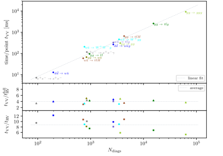
Figure 1: Computation time for selected SM processes with massless fermions. For processes with external $e^{\pm}$, QED corrections were considered, for all other processes QCD corrections. Fermions in loops are considered massless, except for the top which is included in processes with an external top.

In order to estimate the CPU cost of this algorithm in relation to a full NNLO calculation, we compare it to the construction time for the tensor coefficients of the real–virtual contribution, $t_{\scriptscriptstyle{\text{RV}}}$, and for the full real-virtual probability density, $t_{\scriptscriptstyle{\text{RV}}}^{\scriptscriptstyle{\text{full}}}$, including the one-loop tensor integrals. The lower plots of Fig. 1, show approximately constant ratios for the considered processes with $t_{\scriptscriptstyle{\text{VV}}}/t_{\scriptscriptstyle{\text{RV}}}=9\pm 3$ and $t_{\scriptscriptstyle{\text{VV}}}/t_{\scriptscriptstyle{\text{RV}}}^{\scriptscriptstyle{\text{full}}}=4\pm 1$. We conclude that the cost of the double-virtual and real-virtual tensor coefficient construction is comparable, in particular considering that more evaluations of the real-virtual part are usually required during a Monte Carlo integration over the phase space.

The implementation of the algorithm also shows high numerical stability, as demonstrated by relative uncertainty measurements for $2\to 2$ and $2\to 3$ QCD amplitudes computed in double precision for $10^{5}$ uniform random points. These relative uncertainties are in the range of $10^{-16}$ to $10^{-14}$ for the bulk of the points, and never below order $10^{-12}$ and $10^{-11}$ (for details see [1]).

5 Conclusion

We presented a new and completely generic algorithm for the CPU efficient and numerically stable construction of the loop-momentum tensor coefficients of two-loop amplitudes. This constitutes a key building block in the development of an automated two-loop OpenLoops tool.

References

- [1] S. Pozzorini, N. Schär and M. F. Zoller, Two-loop tensor integral coefficients in OpenLoops, JHEP 05 (2022) 161 [2201.11615].
- [2] F. Cascioli, P. Maierhöfer and S. Pozzorini, Scattering Amplitudes with Open Loops, Phys.Rev.Lett. 108 (2012) 111601 [1111.5206].
- [3] F. Buccioni, S. Pozzorini and M. Zoller, On-the-fly reduction of open loops, Eur. Phys. J. C 78 (2018) 70 [1710.11452].
- [4] F. Buccioni, J.-N. Lang, J. M. Lindert, P. Maierhöfer, S. Pozzorini, H. Zhang et al., OpenLoops 2, Eur. Phys. J. C 79 (2019) 866 [1907.13071].
- [5] G. Ossola, C. G. Papadopoulos and R. Pittau, On the Rational Terms of the one-loop amplitudes, JHEP 05 (2008) 004 [0802.1876].
- [6] P. Draggiotis, M. V. Garzelli, C. G. Papadopoulos and R. Pittau, Feynman Rules for the Rational Part of the QCD 1-loop amplitudes, JHEP 04 (2009) 072 [0903.0356].
- [7] M. V. Garzelli, I. Malamos and R. Pittau, Feynman rules for the rational part of the Electroweak 1-loop amplitudes, JHEP 01 (2010) 040 [0910.3130].
- [8] R. Pittau, Primary Feynman rules to calculate the epsilon-dimensional integrand of any 1-loop amplitude, JHEP 02 (2012) 029 [1111.4965].
- [9] A. Denner, S. Dittmaier and L. Hofer, Collier: a fortran-based Complex One-Loop LIbrary in Extended Regularizations, Comput. Phys. Commun. 212 (2017) 220 [1604.06792].
- [10] A. van Hameren, OneLOop: For the evaluation of one-loop scalar functions, Comput.Phys.Commun. 182 (2011) 2427 [1007.4716].
- [11] S. Pozzorini, H. Zhang and M. F. Zoller, Rational Terms of UV Origin at Two Loops, JHEP 05 (2020) 077 [2001.11388].
- [12] J.-N. Lang, S. Pozzorini, H. Zhang and M. F. Zoller, Two-Loop Rational Terms in Yang-Mills Theories, JHEP 10 (2020) 016 [2007.03713].
- [13] J.-N. Lang, S. Pozzorini, H. Zhang and M. F. Zoller, Two-loop rational terms for spontaneously broken theories, JHEP 01 (2022) 105 [2107.10288].