Extreme Love in the SPA: constraining the tidal deformability of supermassive objects with extreme mass ratio inspirals and semi-analytical, frequency-domain waveforms

Abstract

We estimate the accuracy in the measurement of the tidal Love number of a supermassive compact object through the detection of an extreme mass ratio inspiral (EMRI) by the future LISA mission. A nonzero Love number would be a smoking gun for departures from the classical black hole prediction of General Relativity. We find that an EMRI detection by LISA could set constraints on the tidal Love number of a spinning central object with dimensionless spin $\hat{a}=0.9$ ($\hat{a}=0.99$) which are approximately four (six) orders of magnitude more stringent than what achievable with current ground-based detectors for stellar-mass binaries. Our approach is based on the stationary phase approximation to obtain approximate but accurate semi-analytical EMRI waveforms in the frequency-domain, which greatly speeds up high-precision Fisher-information matrix computations. This approach can be easily extended to several other tests of gravity with EMRIs and to efficiently account for multiple deviations in the waveform at the same time.

I Introduction

During a binary inspiral, the tidal interactions between two compact objects become increasingly more relevant. The gravitational field of each object produces a tidal field on its companion, deforming its shape and multipolar structure. This effect can be quantified in terms of tidal-induced multipole moments, more commonly known as the tidal Love numbers (TLNs) [1].

A remarkable result in General Relativity (GR) is that the TLNs of BHs are precisely zero. This was first demonstrated for nonrotating BHs [2, 3, 4, 5] then extended for slowly rotating BHs [6, 7, 8], and more recently it has been proved for Kerr BHs without any approximations [17, 18, 19]. This is generically not the case for BHs in modified gravity and for dark ultracompact objects without a horizon [20], such as boson stars [20, 21, 22], gravastars [23, 20, 24], anisotropic stars [25] and other simple exotic compact objects [26] with stiff equation of state at the surface [20]. In some cases it was found that the TLNs vanish only logarithmically as a function of the compactness in the BH limit [20], providing a “magnifying glass” for near-horizon physics [12, 27].

Beside posing an intriguing problem of “naturalness” in Einstein’s theory [28] and being associated with special emerging symmetries [29, 30, 31, 32], the precise cancellation of the TLNs for BHs in GR also provides an opportunity to test the prediction that all compact objects above a certain mass must be BHs: measuring a nonvanishing TLN would provide a smoking gun for GR deviations or for the existence of new species of ultracompact massive objects. The latter possibility is particularly relevant for supermassive objects which, in the standard paradigm, can only be BHs.

It has been recognized that, for extreme mass-ratio inspirals (EMRIs), the TLNs of the central object affect the gravitational waveform at the leading order in the mass ratio [33]. This property was used to estimate very stringent constraints on the TLNs through an EMRI detection, as achievable by the future space mission LISA [34, 35, 36] and also by third-generation detectors such as the Einstein Telescope [37, 38, 39]. However, the estimates in Ref. [33] were based on a Newtonian computation and a hand-waiving GW dephasing argument which neglects correlations among different waveform parameters. The latter can jeopardize the detectability of a given effect even when the corresponding dephasing is significant [40].

The scope of this paper is to perform a proper estimate of the measurability of the TLNs in an EMRI signal. We shall focus on circular equatorial orbits, but include the spin of both binary components (henceforth the primary and the secondary). Beside being unavoidably present in the waveform, including the spin of the secondary in our context is also useful to understand whether a putatively small effect such as that induced by the tidal deformability of the primary can be confused by other small effects like those induced by the secondary spin.

We shall use the Fisher information matrix, which require to efficiently compute numerical derivatives of the waveform in terms of some of its parameters. For EMRIs, this task is highly delicate and time consuming [41, 42, 43, 40]. To overcome known difficulties related with the inversion of the Fisher matrix and with the numerical derivatives, here we implement a semi-analytical approximation of the waveform using the stationary phase approximation (SPA) [44, 45, 46], which provides an accurate description in the frequency domain. Although we apply this method to the estimate of the TLNs, we envisage that the same approach (with all its benefits) can be directly used for the many other tests of gravity with EMRIs [41, 35, 36, 47].

Our main result is to confirm LISA’s unique power in constraining the TLNs of a supermassive objects [33]. Although our projected bounds are, as expected, less optimistic than those naively derived in Ref. [33], they remain remarkable: as detailed below we find that an EMRI detection with LISA at signal-to-noise ratio (SNR) equal $30$ could constrain the TLNs of a highly-spinning supermassive object up to six orders of magnitude better than what currently achievable with LIGO/Virgo for stellar-mass binaries [48].

We use $G=c=1$ units throughout and the notation follows that of Ref. [49].

II Setup

Before providing the details of our model, it is useful to recall the general argument presented in Ref. [33]. Therein, it was recognized that, at leading post-Newtonian (PN) order and in the small mass-ratio limit ($q\ll 1$), the tidal correction to the instantaneous GW phase reads

$$\phi_{\rm tidal}(f)\propto\frac{k_{1}}{q}v^{5}\,,$$ (1)

where $k_{1}$ is the (quadrupolar, electric) TLN of the primary, $f$ is the GW frequency, $v=(\pi Mf)^{1/3}$, and $M$ is the mass of the primary. Thus, this correction enters at the same (adiabatic) order in the mass ratio as the ordinary radiation-reaction term, $\phi_{N}(f)\propto v^{-5}/q$, while being suppressed relative to the latter by a relative 5PN ($v^{10}$) factor. If $k_{1}\gg q$, the tidal contribution is larger that the first-order correction due to the conservative part of the self force [50, 51], which is instead suppressed by a factor ${\cal O}(q)$ relative to $\phi_{N}$.

This hand-waiving argument is based on a PN expansion, which is known to converge poorly in the extreme mass-ratio limit [52, 53, 54]. On the other hand, it is intriguing that the 5PN suppression of the tidal term might not be relevant for an EMRI, since most of the signal is accumulated at the innermost stable circular orbit (ISCO), when $v={\cal O}(1)$ and the orbital distance $r={\cal O}(M)$.

With this motivation in mind, below we provide a more detailed model to incorporate tidal effects in EMRIs.

II.1 A model for a Kerr-like deformable object

The vacuum region outside a spinning object is not necessarily described by a Kerr geometry due to the absence of Birkhoff’s theorem beyond spherical symmetry. However, in the BH limit, any deviation from the multipolar structure of a Kerr BH dies off sufficiently fast [55] within GR or in modified theories of gravity whose effects are confined near the radius of the compact object. Explicit examples of this “hair-conditioner theorem” [55] within GR are given in Refs. [23, 58, 24, 59, 60, 61], whereas examples in low-energy effective string theory were recently studied in the context of BH microstate geometries in Refs. [62, 63, 64]. In this regime, we assume that the background geometry of the primary is described by the Kerr metric (see e.g. [65, 66] for similar models), given in Boyer-Lindquist coordinates by

$$ds^{2}= -dt^{2}+\Sigma(\Delta^{-1}dr^{2}+d\theta^{2})+(r^{2}+a^{2})\sin^{2}\theta d\phi^{2}$$

$$+\frac{2Mr}{\Sigma}(a\sin^{2}\theta d\phi-dt)^{2}\ ,$$ (2)

where $\Delta=r^{2}-2Mr+a^{2}$, $\Sigma=r^{2}+a^{2}\cos^{2}\theta$, and $a$ is the spin parameter such that $|a|\leq M$. Without loss of generality, we consider the spin of the primary to be aligned with the $z$-axis, namely $a\geq 0$. However, at variance with the standard BH picture, we will allow the object to be deformable when immersed in an external tidal field, in the sense that its TLNs are nonzero.

Note that this model is conservative since, besides including a nonzero TLN, the rest of the geometry is identical to that of a Kerr BH. In specific models of deformable supermassive objects one would generically expect also other deviations, such as tidal heating and deformed multipole moments (see [26] for a review).

II.2 Orbital dynamics and radiation reaction effects

We focus on circular, equatorial, and prograde orbits, for which the initial angular momentum $L_{z}$ is positive and parallel to the $z$-axis. To avoid the complications induced by spin precession, we assume that also the secondary spin is (anti)-aligned with the primary spin.

The EMRI orbital evolution is driven by adiabatic Teukolsky fluxes [67], including linear corrections due to the secondary spin. The radiation reaction equations for the evolution of the orbital parameters are expanded in the mass ratio, and include the contributions due to the TLN of the primary. As explained below, the latter are included in a PN fashion. Although this hybrid model combines elements of BH perturbation theory with PN terms, it allows describing the EMRI dynamics in the strong field regime near the primary, at variance with a fully PN description of the orbital dynamics that instead breaks down near the ISCO.

The orbital motion of a spinning point particle in Kerr spacetime features two integrals of motion: the normalized energy $\tilde{E}=E/\mu$ and angular momentum $\tilde{J}_{z}=J_{z}/(\mu M)$ [68], where $\mu=qM\ll M$ is the secondary mass. To characterize the intrinsic angular momentum of the secondary, we introduce the dimensionless parameter

$$\sigma=\frac{S}{\mu M}=\chi q\ ,$$ (3)

where $\chi=S/\mu^{2}$ is the reduced spin of the secondary. For EMRIs, $|\chi|\ll 1/q$, which implies $|\sigma|\ll 1$. This allows us to expand both $\tilde{E}$ and $\tilde{J}_{z}$ in terms of the spin parameter, considering linear corrections only,

$$\tilde{E} =\tilde{E}^{0}+\sigma\tilde{E}^{1}\quad\ ,\quad\tilde{J}_{z}=\tilde{J}_{z}^{0}+\sigma\tilde{J}_{z}^{1}\,.$$ (4)

The explicit expressions of $\tilde{E}$ and $\tilde{J}_{z}$ are given in [40]. We add to the binding energy $\tilde{E}$ the PN contribution $\tilde{E}_{\textnormal{TLN}}$ due to the TLN of the primary ($k_{1}$) in the point-particle limit [69, 33]

$$\tilde{E}_{\textnormal{TLN}}\simeq-\tilde{E}_{\textnormal{PN}}\bigg{(}\frac{6}{\hat{r}^{5}}+\frac{88}{3}\frac{1}{\hat{r}^{6}}\bigg{)}k_{1}\ ,$$ (5)

with $\tilde{E}_{\textnormal{PN}}=-q/(2\hat{r})$ being the leading-order binding energy in the PN expansion. In the above expression, we included both 5PN and 6PN tidal terms [70]. Note that the secondary TLN ($k_{2}$) would contribute Eq. (5) with terms scaling as $q^{4}$ [33], thus being largely subdominant for the EMRI case. The orbital frequency $\widehat{\Omega}$ is given by

$$\widehat{\Omega}(\hat{r})=\widehat{\Omega}^{0}(\hat{r})+\sigma\widehat{\Omega}^{1}(\hat{r})\ ,$$ (6)

where $\widehat{\Omega}^{0}(\hat{r})=1/(\hat{a}\pm\hat{r}^{3/2})$ is the Keplerian frequency for a nonspinning particle, and

$$\widehat{\Omega}^{1}(\hat{r})=-\frac{3}{2}\frac{\sqrt{\hat{r}}\mp\hat{a}}{\sqrt{\hat{r}}(\hat{r}^{3/2}\pm a)^{2}}\,.$$ (7)

Once the orbital radius $\hat{r}$ and the parameters $\hat{a}$ and $\sigma$ are specified, the orbital dynamics is completely determined by $\tilde{E},\tilde{J}_{z}$, and $\widehat{\Omega}$.

At the adiabatic level, the rate of change of the constants of motion $\tilde{E}$ and $\tilde{J}_{z}$ is balanced by the emitted GW fluxes, in which post-adiabatic corrections induced by the secondary spin are included as described in Ref. [40]. These balance laws hold at first order in $\sigma$ for a spinning particle [71]. The energy fluxes can also be expanded in $\sigma$ at fixed spins $\hat{a}$ and orbital radius $\hat{r}$ [40]:

$$\mathcal{F}(\hat{r},\widehat{\Omega})=\mathcal{F}^{0}(\hat{r},\widehat{\Omega}^{0})+\sigma\mathcal{F}^{1}(\hat{r},\widehat{\Omega}^{0},\widehat{\Omega}^{1})+\mathcal{F}_{\rm TLN}(\hat{r})\,,$$ (8)

where

$$\mathcal{F}^{0}+\sigma\mathcal{F}^{1} =\frac{1}{q}\Bigg{[}\bigg{(}\frac{\mathrm{d}\tilde{E}}{\mathrm{d}\hat{t}}\bigg{)}^{\!\!H}_{\!\!\text{GW}}+\bigg{(}\frac{\mathrm{d}\tilde{E}}{\mathrm{d}\hat{t}}\bigg{)}^{\!\!\infty}_{\!\!\text{GW}}\Bigg{]}\ ,$$ (9)

with $\left(\mathrm{d}\tilde{E}/\mathrm{d}\hat{t}\right)^{\!\!H,\infty}_{\!\!\text{GW}}$ being the energy flux across the horizon and at infinity, respectively, as computed solving Teukolsky’s equations. The tidal contribution to the flux reads

$$\mathcal{F}_{\textnormal{TLN}}(\hat{r})=\frac{128}{5}\frac{k_{1}}{\hat{r}^{10}}\Big{(}1-\frac{22}{21}\frac{1}{\hat{r}}\Big{)}\ ,$$ (10)

where again we have included both 5PN and 6PN corrections. Equation (10) shows that the TLN of the primary contributes to the GW fluxes at the leading, adiabatic, order in $q$ [33].

By defining

$$\mathcal{G}(\hat{r},\widehat{\Omega})\coloneqq\bigg{(}\frac{\mathrm{d}\tilde{E}}{\mathrm{d}\hat{r}}\bigg{)}^{\!-1}\mathcal{F}(\hat{r},\widehat{\Omega})\ ,$$ (11)

then, at first order in the mass ratio,

$$\mathcal{G}(\hat{r},\widehat{\Omega})=\mathcal{G}^{0}(\hat{r},\widehat{\Omega}^{0})+\sigma\mathcal{G}^{1}(\hat{r},\widehat{\Omega}^{0},\widehat{\Omega}^{1})+\mathcal{G}_{\mathrm{TLN}}\,,$$ (12)

$$\mathcal{G}^{0}=\bigg{(}\frac{\mathrm{d}\tilde{E}^{0}}{\mathrm{d}\hat{r}}\bigg{)}^{\!-1}\big{(}\mathcal{F}^{0}+\mathcal{F}_{\textnormal{TLN}}\big{)}\,,$$ (13)

$$\mathcal{G}^{1}=\bigg{(}\frac{\mathrm{d}\tilde{E}^{0}}{\mathrm{d}\hat{r}}\bigg{)}^{\!-1}\mathcal{F}^{1}-\bigg{(}\frac{\mathrm{d}\tilde{E}^{0}}{\mathrm{d}\hat{r}}\bigg{)}^{\!-2}\bigg{(}\frac{\mathrm{d}\tilde{E}^{1}}{\mathrm{d}\hat{r}}\bigg{)}\big{(}\mathcal{F}^{0}+\mathcal{F}_{\rm TLN}\big{)}\,,$$ (14)

$$\mathcal{G}_{\mathrm{TLN}}=-\bigg{(}\frac{\mathrm{d}\tilde{E}^{0}}{\mathrm{d}\hat{r}}\bigg{)}^{\!-2}\bigg{(}\frac{\mathrm{d}\tilde{E}_{\mathrm{TLN}}}{\mathrm{d}\hat{r}}\bigg{)}\big{(}\mathcal{F}^{0}+\mathcal{F}_{\rm TLN}\big{)}\,,$$ (15)

which yield for the time evolution of the orbital radius

$$\frac{\mathrm{d}\hat{r}}{\mathrm{d}\hat{t}}=-q\big{[}\mathcal{G}^{0}(\hat{r},\widehat{\Omega}^{0})+\sigma\mathcal{G}^{1}(\hat{r},\widehat{\Omega}^{0},\widehat{\Omega}^{1})\big{]}\,.$$ (16)

Likewise, at first order in $\sigma$ the orbital phase is given by

$$\frac{\mathrm{d}\phi}{\mathrm{d}\hat{t}}=\widehat{\Omega}^{0}(\hat{r})+\sigma\widehat{\Omega}^{1}(\hat{r})\,.$$ (17)

Solving Eqs. (16) and (17) and linearizing them in $\sigma$ yields the time evolution of $\hat{r}(\hat{t})$ and $\phi(\hat{t})$, which provide the basic ingredients to compute the GW signal emitted by the binary. We compute the Teukolsky fluxes (9) using the same setup and procedure detailed in Refs. [72, 49, 40]. Likewise, the time evolution of $\hat{r}(\hat{t})$ and $\phi(\hat{t})$ is performed as detailed in Ref. [40].

II.3 Time-domain waveform

We use the quadrupole approximation for the GW strain [67]:

$$h_{\alpha}(t) =\frac{2\mu}{D}\widehat{\Omega}(t)^{2/3}\Big{[}A^{+}_{\alpha}(t)\cos(2\phi(t)+2\phi_{0})+$$

$$+A^{\times}_{\alpha}(t)\sin(2\phi(t)+2\phi_{0})\Big{]}\,,$$ (18)

where $\alpha=I,II$ identifies two independent Michelson-like detectors that constitute LISA’s response [73],

$$A^{+}_{\alpha}(t) =(1+\cos^{2}\vartheta)F^{+}_{\alpha}(t)\,,$$ (19)

$$A^{\times}_{\alpha}(t) =-2\cos\vartheta F^{\times}_{\alpha}(t)\,,$$ (20)

where $\phi_{0}$ is the initial orbital phase, $D$ is the source’s luminosity distance from the detector, and $(\vartheta,\varphi)$ identify the direction, in Boyer-Lindquist coordinates, of the latter in a reference frame centered at the source. The antenna pattern functions $F^{+}_{\alpha}(t)$ and $F^{\times}_{\alpha}(t)$ depend on the angles $(\vartheta_{S},\varphi_{S})$ and $(\vartheta_{K},\varphi_{K})$ that provide the direction of the source and of the orbital angular momentum [74] in a heliocentric reference frame attached with the ecliptic [75]. The polar angle $\vartheta$ can be recast in terms of $(\vartheta_{S},\varphi_{S})$ and $(\vartheta_{K},\varphi_{K})$ as

$$\cos\vartheta=\cos\vartheta_{S}\cos\vartheta_{K}+\sin\vartheta_{S}\sin\vartheta_{K}\cos(\varphi_{S}-\varphi_{K})\ .$$ (21)

It is convenient to rewrite Eq. (18) in a more compact form:

$$h_{\alpha}(t) =\frac{2\mu}{D}\widehat{\Omega}(t)^{2/3}\mathcal{A}_{\alpha}(t)\cos(\Phi_{\alpha}(t))\,,$$ (22)

$$\Phi_{\alpha}(t) =2\phi(t)+2\phi_{0}+\phi^{\textup{sh}}_{\alpha}(t)\,,$$ (23)

$$\phi^{\textup{sh}}_{\alpha}(t) =\arctan\bigg{(}-\frac{A^{\times}_{\alpha}(t)}{A^{+}_{\alpha}(t)}\bigg{)}\,,$$ (24)

$$\mathcal{A}_{\alpha}(t) =\sqrt{(A^{+}_{\alpha}(t))^{2}+(A^{\times}_{\alpha}(t))^{2}}\,.$$ (25)

Finally, we include the effect of the Doppler modulation induced by the LISA orbital motion, by introducing a shift in the GW phase:

$$\Phi_{\alpha}(t)\to\Phi_{\alpha}(t)+\phi^{\textup{Dop}}(t)\,,$$ (26)

$$\phi^{\textup{Dop}}(t)=2\Omega(t)R\sin\vartheta_{S}\cos[2\pi(t/T_{{\rm LISA}})-\varphi_{S}]\ ,$$ (27)

where $R=1{\rm AU}$ and $T_{{\rm LISA}}=1\,{\rm yr}$ is LISA’s orbital period [74].

II.4 Frequency-domain waveform in the SPA

We employ the SPA to obtain an approximate but accurate semi-analytical representation of the waveform templates in the frequency domain [44, 45, 46]. The Fourier transform of our time-domain waveform (22) is given as:

$$\tilde{h}_{\alpha}(f)=\frac{\mu}{D}\!\int\limits_{-\infty}^{\infty}\!\!\!\mathrm{d}t\,\widehat{\Omega}(t)^{2/3}\mathcal{A}_{\alpha}(t)e^{-2\pi ift}\big{(}e^{i\Phi_{\alpha}(t)}+e^{-i\Phi_{\alpha}(t)}\big{)}\ ,$$ (28)

and we assume that $\Phi_{\alpha}$ is strictly monotonic in time, i.e. $\dot{\Phi}_{\alpha}(t)>0$. We can rewrite Eq. (28) as

$$\tilde{h}_{\alpha}(f) =\tilde{h}^{+}_{\alpha}(f)+\tilde{h}^{-}_{\alpha}(f)\ ,$$ (29)

$$\tilde{h}^{-}_{\alpha}(f) =\frac{\mu}{D}\!\int\limits_{-\infty}^{\infty}\!\!\!\mathrm{d}t\,\widehat{\Omega}(t)^{2/3}\mathcal{A}_{\alpha}(t)e^{-i(2\pi ft-\Phi_{\alpha}(t))}\ ,$$ (30)

$$\tilde{h}^{+}_{\alpha}(f) =\frac{\mu}{D}\!\int\limits_{-\infty}^{\infty}\!\!\!\mathrm{d}t\,\widehat{\Omega}(t)^{2/3}\mathcal{A}_{\alpha}(t)e^{-i(2\pi ft+\Phi_{\alpha}(t))}\ .$$ (31)

It is sufficient to compute the Fourier transform only for positive frequencies $f$, since our chirp signal is real. The integral $\tilde{h}_{\alpha}(f)$ rapidly oscillates, and the contributions due to the complex exponential cancel out except near the times interval $\tilde{t}$ where the Fourier phase $\Psi_{\alpha}\equiv 2\pi ft-\Phi_{\alpha}(t)$ is stationary:

$$\left.\frac{\mathrm{d}\Psi_{\alpha}}{\mathrm{d}t}\right\rvert_{t=\tilde{t}}=0\implies 2\pi f=\dot{\Phi}_{\alpha}(\tilde{t})\ .$$ (32)

In this case, $\tilde{h}^{+}_{\alpha}$ is negligible [45] , thus $\tilde{h}_{\alpha}\approx\tilde{h}^{-}_{\alpha}$. It is possible then to expand in Taylor series $\Psi_{\alpha}$ near $\tilde{t}$:

$$\Psi_{\alpha}(t)=\Psi_{\alpha}(\tilde{t})+\left.\frac{1}{2}\frac{\mathrm{d}^{2}\Psi_{\alpha}}{\mathrm{d}t^{2}}\right\rvert_{t=\tilde{t}}(t-\tilde{t})^{2}+o\big{(}(t-\tilde{t})^{3}\big{)}\ .$$ (33)

By plugging the above expansion in $\tilde{h}^{-}_{\alpha}(f)$, we obtain the following approximation of $\tilde{h}_{\alpha}(f)$:

$$\tilde{h}_{\alpha}(f)\simeq\frac{\mu}{D}e^{-i(2\pi f\tilde{t}-\Phi_{\alpha}(\tilde{t}))}\!\!\int\limits_{-\infty}^{\infty}\!\!\!\mathrm{d}t\,\widehat{\Omega}(t)^{2/3}\mathcal{A}_{\alpha}(t)e^{-i\frac{1}{2}\ddot{\Phi}_{\alpha}(t-\tilde{t})^{2}}\ .$$ (34)

Before proceeding, we notice that $\Phi_{\alpha}$ includes the terms $\dot{\phi}^{\textup{sh}}(t)$ and $\dot{\phi}^{\textup{Dop}}(t)$, which are suppressed by a factor $2\pi/(\Omega(t)T_{\rm LISA})\ll 1$. Thus, we can safely neglect these terms, approximating $\dot{\Phi}_{\alpha}(t)\approx 2\Omega(t)$. Further assuming that $\mathcal{A}_{\alpha}(t)$ is slowly varying with time, we can write (after a change of variables)

$$\tilde{h}_{\alpha}(f)\simeq\frac{\mu}{D}e^{-i(2\pi f\tilde{t}-\Phi_{\alpha}(\tilde{t}))}(\pi Mf)^{2/3}\mathcal{A}_{\alpha}(\tilde{t})\!\!\int\limits_{-\infty}^{\infty}\!\!\!\mathrm{d}s\,e^{-i\dot{\Omega}(\tilde{t})s^{2}}\ .$$ (35)

The integral in the previous expression can be computed by standard techniques, leading to the SPA for the signal (22)

$$\tilde{h}_{\alpha}(f) =\frac{\mu}{D}(\pi fM)^{2/3}\mathcal{A}_{\alpha}[\tilde{t}(f)]\sqrt{\frac{\pi}{|\dot{\Omega}(\tilde{t}(f))|}}e^{-i\tilde{\Phi}_{\alpha}[\tilde{t}(f)]}\,,$$ (36)

$$\tilde{\Phi}_{\alpha}[\tilde{t}(f)] =2\pi f(\tilde{t}(f)+t_{0})-2(\phi(\tilde{t}(f))+\phi_{0})+$$

$$-\phi^{\textup{Dop}}(\tilde{t}(f))-\phi^{\textup{sh}}_{\alpha}[\tilde{t}(f)]\pm\pi/4\,.$$ (37)

The sign in Eq. (37) is fixed by the sign of the frequency sweep $\dot{\Omega}$, given by

$$\dot{\Omega}=\frac{\mathrm{d}\hat{r}}{\mathrm{d}t}\frac{\mathrm{d}\Omega}{\mathrm{d}\hat{r}}\ ,$$ (38)

while $\tilde{t}(f)$ is the time at which the equation

$$\Omega(t)=\pi f$$ (39)

holds for any given Fourier frequency $f$. The SPA is accurate as long as the amplitude $\mathcal{A}(t)$ and orbital frequency $\Omega(t)$ are slowly varying:

$$\left\lvert\frac{1}{\mathcal{A}_{\alpha}(t)}\frac{\mathrm{d}\mathcal{A}_{\alpha}(t)}{\mathrm{d}t}\right\rvert\sim\frac{\mathcal{O}(10)}{T_{\rm LISA}}\ll|\Omega(t)|\ \ ,\ \left\lvert\frac{\dot{\Omega}(t)}{\Omega(t)^{2}}\right\rvert\ll 1\ .$$ (40)

The first condition is always satisfied since for a typical EMRI $\Omega(t)T_{\rm LISA}\gg{\cal O}(10)$, while we have verified that the second criterion is met for all the binary configurations we analysed. Moreover, the SPA requires $\Omega(t)$ to be strictly monotonic during the orbital evolution. We have checked that this condition is also satisfied in our case (whereas it is not necessarily the case for more general orbits). As a final remark, we note that the frequency-domain waveform is known fully analytically except for the orbital phase $\phi(t)$, the time $\tilde{t}(f)$, and the frequency sweep $\dot{\Omega}(t)$, which have implicit and explicit dependence on the parameters, and needs to be computed numerically.

III Accurate Fisher matrix analysis for EMRI waveforms

The GW signal emitted by a circular, equatorial EMRI with a spinning secondary, moving on the equatorial plane with spin (anti)aligned to the $z$-axis, and including the tidal deformability of the primary, is completely specified by twelve parameters $\vec{y}=\{\vec{y}_{\textnormal{I}},\vec{y}_{\textnormal{E}}\}$: (i) six intrinsic parameters $\vec{y}_{\textnormal{I}}=(\ln\mu,\ln M,\hat{a},\chi,t_{0},k_{1})$ and (ii) six extrinsic parameters $\vec{y}_{\textnormal{E}}=(\phi_{0},\vartheta_{S},\varphi_{S},\vartheta_{K},\varphi_{K},\ln D$). We remind that $(M,\mu)$ are the mass components with $q=\mu/M\ll 1$, $(\hat{a},\chi)$ are the primary and secondary spin parameters, $k_{1}$ is the dimensionless TLN of the primary, $(\phi_{0},\hat{t}_{0})$ define the binary initial phase and starting time, and $D$ is the source luminosity distance. The four angles $(\vartheta_{S},\varphi_{S})$ and $(\vartheta_{K},\varphi_{K})$ correspond to the colatitude and the azimuth of the source sky position and of the orbital angular momentum, respectively [75]. Since the orbit is circular and equatorial, the orbital angular momentum has no precession around the primary spin, and all angular momenta are parallel to each other.

In the limit of large SNR, the errors on the source parameters inferred by a given EMRI observation can be determined using the Fisher information matrix:

$$\Gamma_{ij}=\sum_{\alpha=I,II}\left(\frac{d\tilde{h}_{\alpha}}{dy^{i}}\middle|\frac{d\tilde{h}_{\alpha}}{dy^{j}}\right)_{\vec{y}=\vec{y}_{0}}\ ,$$ (41)

where $\vec{y}_{0}$ corresponds to the true set of binary parameters, and we have introduced the noise-weighted scalar product between two waveforms $p_{\alpha}$ and $q_{\alpha}$ in the frequency domain:

$$(p_{\alpha}|q_{\alpha})=2\int_{f_{\rm min}}^{f_{\rm max}}\frac{df}{S_{n}(f)}[\tilde{p}^{*}_{\alpha}(f)\tilde{q}_{\alpha}(f)+\tilde{p}_{\alpha}(f)\tilde{q}^{*}_{\alpha}(f)]\ ,$$ (42)

where $S_{n}(f)$ corresponds to the noise spectral density of the detector, and the star identifies complex conjugation. The scalar product was computed using the Simpson’s integration method. In our computations we choose $f_{\rm max}$ and $f_{\rm min}$ as

$$f_{\rm min} =\frac{2}{2\pi}\frac{1}{M}\Big{[}\widehat{\Omega}^{0}(\hat{r}_{0})+\sigma\widehat{\Omega}^{1}(\hat{r}_{0})\Big{]}\ ,$$ (43)

$$f_{\rm max} =\frac{2}{2\pi}\frac{1}{M}\Big{[}\widehat{\Omega}^{0}(\hat{r}_{\rm ISCO})+\sigma\widehat{\Omega}^{1}(\hat{r}_{{\rm ISCO}})\Big{]}\ ,$$ (44)

where $\hat{r}_{\rm ISCO}$ is location of the ISCO for a nonspinning test particle around a spinning central object, and $\hat{r}_{0}$ is the initial orbital radius. The waveform scalar product allows us to define the optimal SNR for a given signal $h$:

$${\rm SNR}=(h|h)^{1/2}\,,$$ (45)

which scales linearly with the inverse of the luminosity distance. The inverse of $\Gamma_{ij}$ is the covariance matrix $\Sigma_{ij}$, whose diagonal elements correspond to the statistical uncertainties of the waveform parameters,

$$\sigma^{2}_{x_{i}}=(\Gamma^{-1})_{ii}\ ,$$ (46)

whereas the off-diagonal elements correspond to the correlation coefficients. In the large-SNR limit the covariance matrix scales inversely with the SNR. For a given set of parameters, it is therefore straightforward to rescale the errors by varying the luminosity distance $D$, and hence the SNR.

In addition to the standard deviations on the twelve parameters defined above, we also analyze the error box on the solid angle spanned by the unit vector associated to $(\vartheta_{S},\varphi_{S})$ and $(\vartheta_{K},\varphi_{K})$:

$$\Delta\Omega_{i}=2\pi|\sin\vartheta_{i}|\sqrt{\sigma^{2}_{\vartheta_{i}}\sigma^{2}_{\varphi_{i}}-\Sigma^{2}_{\vartheta_{i}\varphi_{i}}}\ .$$ (47)

where $i=(S,K)$.

As discussed in [40], the inclusion of the secondary spin can severely deteriorate the accuracy with which the other intrinsic parameters are recovered. For this reason, we consider three alternatives scenarios in our data analysis: (i) the secondary spin $\chi$ is an unbounded parameter, (ii) a suitable prior is applied to $\chi$, (iii) the secondary spin is integrated out from the posterior distribution, by simply removing the corresponding row and column from the Fisher matrix.

For case (ii) we assume a wide prior given by a Gaussian probability distribution with standard deviation $\sigma_{0}=1$ and zero mean. In this configuration the errors on the source parameters are given by

$$\sigma^{2}_{x_{i}}=\Sigma_{ii}=[(\Gamma+\Gamma_{0})^{-1}]_{ii}\ ,$$ (48)

where $(\Gamma_{0})_{ij}=1/\sigma_{0}\delta_{i\chi}\delta_{\chi j}$ is the Fisher matrix corresponding to the prior distribution [40].

We have computed the numerical integral in Eq. (42) assuming the LISA sensitivity curve, including the contribution of the confusion noise from the unresolved Galactic binaries [76]. The numerical derivatives of the waveform with respect to the parameters, required to compute the Fisher matrix, are computed as explained in Appendix A, whereas the numerical stability of the Fisher and covariance matrices is discussed in Appendix B.

We consider $T=1\,{\rm yr}$ observation time, with the orbital evolution actually ending not exactly at the $\hat{r}_{\rm ISCO}$, but at the onset of the transition region as defined in [77], i.e. $r_{\textnormal{plunge}}=\hat{r}_{\textup{ISCO}}+\delta\hat{r}$ with $\delta\hat{r}=4q^{2/5}$. We fix the injected angles to the fiducial values $\vartheta_{S}=\pi/4,\phi_{S}=0,\vartheta_{K}=\pi/8,\phi_{K}=0$. We focus on binaries with component masses $M=10^{6}M_{\odot}$ and $\mu=10M_{\odot}$, secondary spin $\chi=0$, setting the primary TLN to $k_{1}=0$. Finally, the luminosity distance is scaled such that the binary has ${\rm SNR}=30$ for any spin.

IV Results and discussion

IV.1 Comparison between the fast Fourier transform and the SPA

We have checked the validity of the SPA by computing the faithfulness between EMRI waveforms in the frequency domain obtained in two differnt ways: (i) with a fast Fourier transform (FFT) of the time signal (22), and (ii) with the SPA presented above. Specifically, we compute

$$\mathscr{F}(h^{\rm{SPA}}_{\alpha},h^{\rm{FFT}}_{\alpha})=\underset{t_{0},\phi_{0}}{\max}\frac{(h^{\rm{SPA}}_{\alpha}|h^{\rm{FFT}}_{\alpha})}{\sqrt{(h^{\rm{SPA}}_{\alpha}|h^{\rm{SPA}}_{\alpha})(h^{\rm{FFT}}|h^{\rm{FFT}})}}\ .$$ (49)

Following the Shannon theorem, for the FFT we use a sampling time $\Delta t_{s}=\lfloor 1/(2f_{\rm max})-1\rfloor$, with $n_{s}=T/\Delta t_{s}$ being the total number of samples, $T=1\textnormal{yr}$, and $f_{\textnormal{max}}$ given by Eq. (44). Before applying the FFT we have tapered the time domain signal to reduce spectral leakage, using a Tukey window with window size $\beta=0.001$.

Table 1 provides the values of the faithfulness computed for two configurations of the primary spin, and for each LISA channel. In agreement with [44], our results show that the SPA waveform model matches well with the FFT waveform: $\mathscr{F}(h^{\rm{SPA}}_{\alpha},h^{\rm{FFT}}_{\alpha})\gtrsim 0.993$ even for a highly-spinning primary with $\hat{a}=0.99$. As a useful rule of thumb, values of $\mathscr{F}$ smaller than $\mathscr{F}\sim 1-\frac{{\cal D}}{{2\rm SNR}^{2}}$, with ${\cal D}$ dimension of the waveform model, highlights that two templates differ significantly among each other [78, 79]. For ${\cal D}=12$ as in our case, this threshold translates into $\mathscr{F}\sim 0.993$ for SNR=30, so the SPA is sufficiently accurate for a typical EMRI SNR.

As a further assessment of the validity of the SPA, we have compared the standard deviations (46), obtained with the SPA and with the frequency-domain waveforms computed through a FFT. In the last case derivatives of the template with respect to the binary parameters have been numerically determined using a five-point stencil formula (see Ref. [40] for details), except for the luminosity distance $D$, since $\partial\tilde{h}(f)/\partial D$ can be computed analytically. In the worst case scenario we find that the maximum relative difference between the standard deviations provided by the Fisher matrix are: (i) $\sim 15\%$ when $\chi$ is unbounded, (ii) $\sim 3\%$ when the secondary spin is excluded, (iii) $\sim 2\%$ when a prior on $\chi$ is imposed. Overall, these results confirm that the SPA provides a reliable and accurate analytic approximation of the purely numerically frequency-domain waveforms employed for EMRIs.

$\hat{a}$	channel	$\mathscr{F}$
0.9	I	0.9931
	II	0.9970
0.99	I	0.9942
	II	0.9971

Table 1: Faithfulness $\mathscr{F}(h^{\rm{SPA}}_{\alpha},h^{\rm{FFT}}_{\alpha})$ between frequency-domain waveforms obtained with the SPA, and by applying the FFT to the time domain signal, for different values of the primary spin parameter $\hat{a}$ and for our reference binary system. The second column identifies the independent channels of the LISA interferometer. We consider EMRIs evolving for one-year up to the plunge.

IV.2 Measurability of the TLN

We now present our main results for the measurability of the primary TLN, $k_{1}$. In Table 2, we provide the statistical errors on the waveform parameters when both the 5PN and the 6PN tidal corrections are included in the waveform. We first notice that $k_{1}$ can be detected with high accuracy even when the secondary spin $\chi$ is considered as an unbounded parameter (first row of Table 2). The marginalization of $\chi$ (second row) or the inclusion of a Gaussian prior on $\chi$ (third row) improves the statistical error on all intrinsic parameters ($\ln M,\ln\mu,\hat{a}$, and $k_{1}$).

We have also checked that including only the leading PN order (5PN) tidal term does not affect significantly the standard deviations on the parameters. This fact provides a good consistency check of our hybrid waveform (mixing BH perturbation theory with PN corrections), since the PN series is not supposed to converge near the ISCO of a highly-spinning BH. We can therefore expect that higher-order tidal terms (or a resummation thereof) would not change our results significantly.

We find that the TLN of the primary $k_{1}$ can be constrained with the astonishing accuracy of above $3\times 10^{-2}$ and $8\times 10^{-4}$ for $\hat{a}=0.9$ and $\hat{a}=0.99$, respectively. As a figure of merit, it is interesting to note that so far the only measurement of the tidal deformability of a compact object is that coming from GW170817 [48], which set a constraint on the TLN of a neutron star at the level of $\sigma_{k_{1}}\lesssim 10^{3}$, i.e. several orders of magnitude less stringent than what achievable with EMRIs. It is also interesting to note that, for all models of compact objects in which the TLNs scale logarithmically with the compactness [20], $\sigma_{k_{1}}\sim 10^{-3}$ would allow to probe putative structure at Planckian distance from the horizon and to distinguish between different proposals of exotic compact objects motivated by quantum gravity [11, 80, 12].

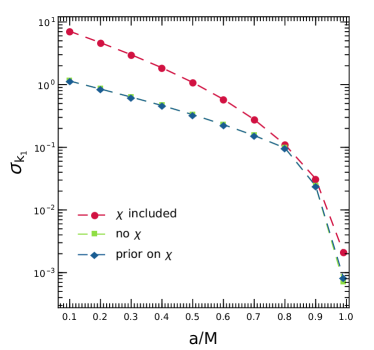
Figure 1: 1-$\sigma$ error on the primary TLN $k_{1}$ as a function of the primary spin parameter $\hat{a}\in[0.1,0.99]$. Different markers correspond to including the spin of the secondary, removing it from the Fisher matrix, or adding a Gaussian prior centered around the injected value of $\chi$ (see main text). The luminosity distance is fixed such that ${\rm SNR}=30$ after 1 year of observation. As a reference, current measurement errors on the TLN of a neutron star coming from GW170817 [48] are $\sigma_{k_{1}}\lesssim 10^{3}$.

Finally, Fig.1 shows the statistical error on $k_{1}$ for different values of the primary spin $\hat{a}$ and different assumptions for the secondary spin. We observe that the error decreases very rapidly as the primary spin increases, because the majority of the signal comes from the ISCO of the highly-spinning primary, where tidal effects are more relevant. As stressed above, since the PN series poorly converges near the ISCO, it is important that the results shown in Fig.1 (which includes the 6PN tidal corrections) are very similar to those one would obtain by including only the 5PN terms. Furthermore, Fig.1 confirms that neglecting the secondary spin or including it with a very conservative prior gives almost identical results. Thus, the secondary spin does not hamper the ability of measuring a nonstandard small effect such as the primary tidal deformability.

5PN and 6PN TLN terms    $\hat{a}_{\text{injected}}=0.9$
prior	$\ln M$	$\ln\mu$	$\hat{a}$	$\chi$	$\hat{t}_{0}$	$k_{1}$	$\phi_{0}$	$\ln D$	$\Delta\Omega_{S}$	$\Delta\Omega_{K}$
no	-4.9	-4.1	-3.8	1.6	0.48	-1.5	0.74	-0.069	$6.2\times 10^{-4}$	7.5
no	-5.8	-4.2	-4.1	–	0.48	-1.6	0.74	-0.069	$5.9\times 10^{-4}$	2.9
yes	-5.7	-4.2	-4.1	0.57	0.48	-1.6	0.74	-0.069	$5.9\times 10^{-4}$	7.5
5PN and 6PN TLN terms    $\hat{a}_{\text{injected}}=0.99$
prior	$\ln M$	$\ln\mu$	$\hat{a}$	$\chi$	$\hat{t}_{0}$	$k_{1}$	$\phi_{0}$	$\ln D$	$\Delta\Omega_{S}$	$\Delta\Omega_{K}$
no	-5.2	-4.6	-4.4	1.2	0.21	-2.7	0.74	-0.071	$2.7\times 10^{-4}$	6.7
no	-5.8	-4.9	-5.0	–	0.21	-3.1	0.74	-0.071	$2.7\times 10^{-4}$	2.6
yes	-5.7	-4.8	-4.9	0.61	0.21	-3.1	0.74	-0.071	$2.7\times 10^{-4}$	6.7

Table 2: Top: Fisher-matrix errors on the intrinsic source parameters, on the luminosity distance, and on the solid angles which define the orientation and the orbital angular momentum of the binary for our model. The primary has spin $\hat{a}=0.9$ while the secondary is nonspinning, with $M=10^{6}M_{\odot}$, $\mu=10M_{\odot}$, and $k_{1}=0$. For clarity, we present the $\log_{10}$ of the errors on $\ln M$, $\ln\mu$, $\hat{a}$, $\chi$, $\hat{t}_{0}$, $k_{1}$, $\phi_{0}$, and $\ln D$. We include both the 5PN and 6PN TLN terms. Bottom: same as the top but with $\hat{a}=0.99$. The SNR for a source at $D=1\,{\rm Gpc}$ is ${\rm SNR}=111$ (top) and ${\rm SNR}=125$ (bottom), but the errors are all normalized to the fiducial value ${\rm SNR}=30$.

V Conclusion

Measuring a nonzero TLN for a supermassive object would be a robust smoking gun for new physics beyond the standard BH prediction in GR. EMRIs detectable by LISA are unique sources for tests of gravity and allow for unparalleled measurements of beyond-GR effects. With these motivations in mind, we have estimated the accuracy in the measurement of the tidal deformability of a supermassive compact object through an EMRI detection by LISA. Confirming back-of-the-envelope estimates [33], we found the TLN of the central supermassive object can be measured at the level of $10^{-3}$ if the central object is highly spinning. This is about 6 orders of magnitude better than current accuracy in measuring the TLNs of a NS with ground-based detectors.

We included the secondary spin as a possible source of confusion, showing that its inclusion does not affect the bounds on the primary TLN. On the other hand, we have focused on simplified (circular, equatorial, nonprecessing) orbits. It would be important to extend our analysis by including eccentricity, inclined orbits [44, 81, 82], and possible spin precession [83, 84]. On the one hand these extensions will increase the dimensionality of the parameter space, rendering parameter estimation more demanding, but on the other hand they might also help in disentangling possible parameter correlations. Another possible extension would be the inclusion of important post-adiabatic corrections to the waveforms [85, 86, 87, 88]. Finally, we have adopted a hybrid “Teukolsky+PN” waveform, where tidal corrections were introduced with their corresponding (leading and next-to-leading order) PN terms. An interesting extension would be to compute the tidal deformability contribution in the point-particle limit but without PN expansion, by evaluating the tidal tensor of the secondary along its worldline.

As a by-product of our analysis, we have assessed the accuracy of the SPA to perform efficient tests of gravity with EMRI waveforms in the frequency domain. One great advantage of the SPA is that it reduces the number of numerical derivatives required to compute and invert the Fisher matrix, making the error estimate extremely more efficient from a numerical perspective. Although we have applied this approach to the specific case of constraining the TLNs, we expect the same method can be applied to several other tests of gravity. In a future work [89] we will use this approach to constrain a comprehensive parametrized waveform accounting for multiple deviations at the same time.

Appendix A Semi-analytic derivatives of the waveforms

The frequency-domain waveform (36) has an implicit dependence on the intrinsic parameters $\vec{x}\equiv\vec{y}_{I}=(\ln M,\ln\mu,\hat{a},\chi,k_{1})$ through the functions $\tilde{t}(f;\vec{x})$, $\phi(\tilde{t}(f;\vec{x});\vec{x})$ and $\dot{\Omega}(\tilde{t}(f;\vec{x});\vec{x})$. In this appendix we show how to compute the derivatives of the waveforms with respect to the intrinsic parameters $\vec{x}$ in a semi-analytic fashion.

By the theorem of the implicit functions, the derivatives $\partial\tilde{t}(f;\vec{x})/\partial x^{i}$ are given as

$$\frac{\partial\tilde{t}(f;\vec{x})}{\partial x^{i}}=\left.-\frac{1}{\dot{\Omega}(t;\vec{x})}\frac{\partial\Omega(t;\vec{x})}{\partial x^{i}}\right\rvert_{t=\tilde{t}(f;\vec{x})}\ .$$ (50)

The derivatives $\partial\phi(t;\vec{x})/\partial x^{i}$ are instead given as solutions of the following ordinary differential equation with initial condition $\partial\phi(0;\vec{x})/\partial x^{i}=0$:

$$\frac{\mathrm{d}}{\mathrm{d}t}\bigg{(}\frac{\partial\phi(t;\vec{x})}{\partial x^{i}}\bigg{)}=\frac{\partial\Omega(\hat{r}(t;x);\vec{x})}{\partial x^{i}}+\frac{\partial\Omega(\hat{r}(t;x);\vec{x})}{\partial\hat{r}}\frac{\partial\hat{r}(t;\vec{x})}{\partial x^{i}}\ ,$$ (51)

where $\partial\hat{r}(t;\vec{x})/\partial x^{i}$ can be computed from

$$\frac{\mathrm{d}}{\mathrm{d}t}\bigg{(}\frac{\partial\hat{r}(t;\vec{x})}{\partial x^{i}}\bigg{)} =\frac{\partial}{\partial x^{i}}\bigg{(}\frac{\mathrm{d}\hat{r}}{\mathrm{d}t}(\hat{r}(t;\vec{x});\vec{x})\bigg{)}+$$

$$+\frac{\partial}{\partial\hat{r}}\bigg{(}\frac{\mathrm{d}\hat{r}}{\mathrm{d}t}(\hat{r}(t;\vec{x});\vec{x})\bigg{)}\frac{\partial\hat{r}(t;\vec{x})}{\partial x^{i}}$$ (52)

with initial condition $\partial\hat{r}(0;\vec{x})/\partial x^{i}=0$. Finally, the derivatives $\partial\phi(\tilde{t}(f;\vec{x});\vec{x})/\partial x^{i}$ can be written as

$$\frac{\partial\phi(\tilde{t}(f;\vec{x});\vec{x})}{\partial x^{i}} =\left.\frac{\partial\phi(t;\vec{x})}{\partial x^{i}}\right\rvert_{t=\tilde{t}(f;\vec{x})}+\frac{\mathrm{d}\phi(t;\vec{x})}{\mathrm{d}t}\frac{\partial\tilde{t}(f;\vec{x})}{\partial x^{i}}$$

$$=\left.\frac{\partial\phi(t;\vec{x})}{\partial x^{i}}\right\rvert_{t=\tilde{t}(f;\vec{x})}+\pi f\frac{\partial\tilde{t}(f;\vec{x})}{\partial x^{i}}$$ (53)

Therefore, the derivatives $\partial\Phi_{\alpha}(\tilde{t}(f;\vec{x}))/\partial x^{i}$ of the SPA phase (37) are

$$\frac{\partial\tilde{\Phi}_{\alpha}(\tilde{t}(f;\vec{x});\vec{x})}{\partial x^{i}}=\left.-2\frac{\partial\phi(t;\vec{x})}{\partial x^{i}}\right\rvert_{t=\tilde{t}(f;\vec{x})}\ .$$ (54)

Note that the contribution to $\partial\tilde{\Phi}_{\alpha}(\tilde{t}(f;\vec{x}))/\partial x^{i}$ given by $\partial\phi^{\text{sh}}_{\alpha}(\tilde{t}(f;\vec{x}))/\partial x^{i}$ and $\partial\phi^{\text{Dop}}_{\alpha}(\tilde{t}(f;\vec{x}))/\partial x^{i}$ is negligible, since $\Omega(t)T_{\rm LISA}\gg 2\pi$ for a typical EMRI detectable by LISA.

Finally, the derivatives of the frequency sweep $\partial\dot{\Omega}(\tilde{t}(f;\vec{x});\vec{x})/\partial x^{i}$ are given by

$$\frac{\partial\dot{\Omega}(\tilde{t}(f;\vec{x});\vec{x})}{\partial x^{i}}=\left(\left.\frac{\partial\dot{\Omega}(t;\vec{x})}{\partial x^{i}}+\ddot{\Omega}(t;\vec{x})\frac{\partial\tilde{t}(f;\vec{x})}{\partial x^{i}}\right)\right\rvert_{t=\tilde{t}(f;\vec{x})}\ .$$ (55)

Once $\partial\tilde{t}(f;\vec{x}))/\partial x^{i}$, $\partial\Phi_{\alpha}(\tilde{t}(f;\vec{x}))/\partial x^{i}$ and $\partial\dot{\Omega}(\tilde{t}(f;\vec{x});\vec{x})$ are known, the semi-analytic derivatives of the frequency domain template (36) with respect to the binary parameters can be constructed straightforwardly.

Appendix B Stability of the Fisher matrix

In this appendix we provide further details on the accuracy of the calculations we performed, assessing the numerical stability of the covariance matrix for the waveform parameters. This is particularly relevant in the case of EMRIs, for which Fisher matrices are known to be ill-conditioned [90], and small numerical or systematic errors are amplified after computing the inverse. As a rule of thumb, for a condition number $\kappa=10^{n}$, one may lose up to $n$ figures of accuracy, which should be added to the numerical errors.

This problem is exacerbated when finite-difference methods are employed for the waveform derivatives [40, 42], since the covariance matrix can be sensitive to the choice in the parameter shifts adopted for the differentiation. However, the semi-analytic approach described in Appendix A, combined with the SPA, avoids such issues.

Inverting the Fisher matrices still remains a delicate task, which can depend on the numerical precision used for the calculation due to the large condition number. Indeed, for the binary configurations we considered, we find $\kappa\sim 10^{25}$ and $\kappa\sim 10^{18}$, for a primary with $\hat{a}=0.1$ and $\hat{a}=0.99$, respectively.

We have first tested the stability of the Fisher inversion against changes in the numerical precision. In the worst case, which occurs when the secondary spin is included, we find that a stable covariance matrix requires at least 35 digits of precision in input.

Moreover, we have checked the sensitivity of both Fisher and covariance matrices to small variations of their components, by perturbing them with a deviation matrix $F^{ij}$. We draw all elements of $F^{ij}$ from a uniform distribution $U\in[a,b]$, and then compute

$$\delta_{\textit{\rm stability}}\equiv\underset{ij}{\max}\Bigg{[}\frac{\big{(}(\Gamma+F)^{-1}-\Gamma^{-1}\big{)}^{ij}}{(\Gamma^{-1})^{ij}}\Bigg{]}\ .$$ (56)

For the most problematic configurations we analysed:

• the inverse without priors is stable with $\delta_{\textit{\rm stability}}=5\%$ with perturbations $U\in[-10^{-9},10^{-9}]$.

• the inverse with priors is stable with $\delta_{\textit{\rm stability}}=6\%$ with perturbations $U\in[-10^{-6},10^{-6}]$.

• the inverse without secondary spin $\chi$ is stable with $\delta_{\textit{\rm stability}}=2\%$ with perturbations $U\in[-10^{-5},10^{-5}]$.

The stability of the Fisher matrices drastically improves as the spin of the primary increases. For $\hat{a}=0.99$, the inverse is stable with $\delta_{\textnormal{stability}}\lesssim 2\%$ and perturbations $U\in[-10^{-5},10^{-5}]$ for all cases we considered.

References

- [1] E. Poisson and C. Will, Gravity: Newtonian, Post-Newtonian, Relativistic. Cambridge University Press, 2014. https://books.google.it/books?id=PZ5cAwAAQBAJ.
- [2] T. Damour, “Contribution in Gravitational Radiation,” Proceedings Summer School, NATO Advanced Study Institute, Les Houches (1984) .
- [3] T. Binnington and E. Poisson, “Relativistic theory of tidal Love numbers,” Phys. Rev. D 80 (2009) 084018, arXiv:0906.1366 [gr-qc].
- [4] T. Damour and A. Nagar, “Relativistic tidal properties of neutron stars,” Phys. Rev. D 80 (2009) 084035, arXiv:0906.0096 [gr-qc].
- [5] N. Gürlebeck, “No-hair theorem for Black Holes in Astrophysical Environments,” Phys. Rev. Lett. 114 no. 15, (2015) 151102, arXiv:1503.03240 [gr-qc].
- [6] E. Poisson, “Tidal deformation of a slowly rotating black hole,” Phys. Rev. D 91 no. 4, (2015) 044004, arXiv:1411.4711 [gr-qc].
- [7] P. Pani, L. Gualtieri, A. Maselli, and V. Ferrari, “Tidal deformations of a spinning compact object,” Phys. Rev. D 92 no. 2, (2015) 024010, arXiv:1503.07365 [gr-qc].
- [8] P. Landry and E. Poisson, “Tidal deformation of a slowly rotating material body. External metric,” Phys. Rev. D 91 (2015) 104018, arXiv:1503.07366 [gr-qc].
- [9] J. B. Hartle, “Tidal Friction in Slowly Rotating Black Holes,” Phys. Rev. D8 (1973) 1010–1024.
- [10] S. A. Hughes, “Evolution of circular, nonequatorial orbits of Kerr black holes due to gravitational wave emission. II. Inspiral trajectories and gravitational wave forms,” Phys. Rev. D 64 (2001) 064004, arXiv:gr-qc/0104041. [Erratum: Phys.Rev.D 88, 109902 (2013)].
- [11] A. Maselli, P. Pani, V. Cardoso, T. Abdelsalhin, L. Gualtieri, and V. Ferrari, “Probing Planckian corrections at the horizon scale with LISA binaries,” Phys. Rev. Lett. 120 no. 8, (2018) 081101, arXiv:1703.10612 [gr-qc].
- [12] A. Maselli, P. Pani, V. Cardoso, T. Abdelsalhin, L. Gualtieri, and V. Ferrari, “From micro to macro and back: probing near-horizon quantum structures with gravitational waves,” Class. Quant. Grav. 36 no. 16, (2019) 167001, arXiv:1811.03689 [gr-qc].
- [13] S. Datta, R. Brito, S. Bose, P. Pani, and S. A. Hughes, “Tidal heating as a discriminator for horizons in extreme mass ratio inspirals,” Phys. Rev. D 101 no. 4, (2020) 044004, arXiv:1910.07841 [gr-qc].
- [14] E. Maggio, M. van de Meent, and P. Pani, “Extreme mass-ratio inspirals around a spinning horizonless compact object,” Phys. Rev. D 104 no. 10, (2021) 104026, arXiv:2106.07195 [gr-qc].
- [15] N. Sago and T. Tanaka, “Oscillations in the extreme mass-ratio inspiral gravitational wave phase correction as a probe of a reflective boundary of the central black hole,” Phys. Rev. D 104 no. 6, (2021) 064009, arXiv:2106.07123 [gr-qc].
- [16] V. Cardoso and F. Duque, “Resonances, black hole mimickers, and the greenhouse effect: Consequences for gravitational-wave physics,” Phys. Rev. D 105 no. 10, (2022) 104023, arXiv:2204.05315 [gr-qc].
- [17] A. Le Tiec, M. Casals, and E. Franzin, “Tidal Love Numbers of Kerr Black Holes,” Phys. Rev. D 103 no. 8, (2021) 084021, arXiv:2010.15795 [gr-qc].
- [18] H. S. Chia, “Tidal deformation and dissipation of rotating black holes,” Phys. Rev. D 104 no. 2, (2021) 024013, arXiv:2010.07300 [gr-qc].
- [19] A. Le Tiec and M. Casals, “Spinning Black Holes Fall in Love,” Phys. Rev. Lett. 126 no. 13, (2021) 131102, arXiv:2007.00214 [gr-qc].
- [20] V. Cardoso, E. Franzin, A. Maselli, P. Pani, and G. Raposo, “Testing strong-field gravity with tidal Love numbers,” Phys. Rev. D 95 no. 8, (2017) 084014, arXiv:1701.01116 [gr-qc]. [Addendum: Phys.Rev.D 95, 089901 (2017)].
- [21] N. Sennett, T. Hinderer, J. Steinhoff, A. Buonanno, and S. Ossokine, “Distinguishing Boson Stars from Black Holes and Neutron Stars from Tidal Interactions in Inspiraling Binary Systems,” Phys. Rev. D 96 no. 2, (2017) 024002, arXiv:1704.08651 [gr-qc].
- [22] R. F. P. Mendes and H. Yang, “Tidal deformability of boson stars and dark matter clumps,” Class. Quant. Grav. 34 no. 18, (2017) 185001, arXiv:1606.03035 [astro-ph.CO].
- [23] P. Pani, “I-Love-Q relations for gravastars and the approach to the black-hole limit,” Phys. Rev. D 92 no. 12, (2015) 124030, arXiv:1506.06050 [gr-qc]. [Erratum: Phys.Rev.D 95, 049902 (2017)].
- [24] N. Uchikata, S. Yoshida, and P. Pani, “Tidal deformability and I-Love-Q relations for gravastars with polytropic thin shells,” Phys. Rev. D 94 no. 6, (2016) 064015, arXiv:1607.03593 [gr-qc].
- [25] G. Raposo, P. Pani, M. Bezares, C. Palenzuela, and V. Cardoso, “Anisotropic stars as ultracompact objects in General Relativity,” Phys. Rev. D 99 no. 10, (2019) 104072, arXiv:1811.07917 [gr-qc].
- [26] V. Cardoso and P. Pani, “Testing the nature of dark compact objects: a status report,” Living Rev. Rel. 22 no. 1, (2019) 4, arXiv:1904.05363 [gr-qc].
- [27] S. Datta, “Probing horizon scale quantum effects with Love,” arXiv:2107.07258 [gr-qc].
- [28] R. A. Porto, “The Tune of Love and the Nature(ness) of Spacetime,” Fortsch. Phys. 64 no. 10, (2016) 723–729, arXiv:1606.08895 [gr-qc].
- [29] L. Hui, A. Joyce, R. Penco, L. Santoni, and A. R. Solomon, “Static response and Love numbers of Schwarzschild black holes,” JCAP 04 (2021) 052, arXiv:2010.00593 [hep-th].
- [30] P. Charalambous, S. Dubovsky, and M. M. Ivanov, “Hidden Symmetry of Vanishing Love Numbers,” Phys. Rev. Lett. 127 no. 10, (2021) 101101, arXiv:2103.01234 [hep-th].
- [31] P. Charalambous, S. Dubovsky, and M. M. Ivanov, “On the Vanishing of Love Numbers for Kerr Black Holes,” JHEP 05 (2021) 038, arXiv:2102.08917 [hep-th].
- [32] L. Hui, A. Joyce, R. Penco, L. Santoni, and A. R. Solomon, “Ladder symmetries of black holes. Implications for love numbers and no-hair theorems,” JCAP 01 no. 01, (2022) 032, arXiv:2105.01069 [hep-th].
- [33] P. Pani and A. Maselli, “Love in Extrema Ratio,” Int. J. Mod. Phys. D28 no. 14, (2019) 1944001, arXiv:1905.03947 [gr-qc].
- [34] LISA Collaboration, P. Amaro-Seoane et al., “Laser Interferometer Space Antenna,” arXiv:1702.00786 [astro-ph.IM].
- [35] E. Barausse et al., “Prospects for Fundamental Physics with LISA,” Gen. Rel. Grav. 52 no. 8, (2020) 81, arXiv:2001.09793 [gr-qc].
- [36] LISA Collaboration, K. G. Arun et al., “New horizons for fundamental physics with LISA,” Living Rev. Rel. 25 no. 1, (2022) 4, arXiv:2205.01597 [gr-qc].
- [37] M. Maggiore et al., “Science Case for the Einstein Telescope,” JCAP 03 (2020) 050, arXiv:1912.02622 [astro-ph.CO].
- [38] V. Kalogera et al., “The Next Generation Global Gravitational Wave Observatory: The Science Book,” arXiv:2111.06990 [gr-qc].
- [39] S. Barsanti, V. De Luca, A. Maselli, and P. Pani, “Detecting Subsolar-Mass Primordial Black Holes in Extreme Mass-Ratio Inspirals with LISA and Einstein Telescope,” Phys. Rev. Lett. 128 no. 11, (2022) 111104, arXiv:2109.02170 [gr-qc].
- [40] G. A. Piovano, R. Brito, A. Maselli, and P. Pani, “Assessing the detectability of the secondary spin in extreme mass-ratio inspirals with fully relativistic numerical waveforms,” Phys. Rev. D 104 no. 12, (2021) 124019, arXiv:2105.07083 [gr-qc].
- [41] A. Maselli, N. Franchini, L. Gualtieri, T. P. Sotiriou, S. Barsanti, and P. Pani, “Detecting fundamental fields with LISA observations of gravitational waves from extreme mass-ratio inspirals,” Nature Astron. 6 no. 4, (2022) 464–470, arXiv:2106.11325 [gr-qc].
- [42] O. Burke, J. R. Gair, J. Simón, and M. C. Edwards, “Constraining the spin parameter of near-extremal black holes using LISA,” Phys. Rev. D 102 no. 12, (2020) 124054, arXiv:2010.05932 [gr-qc].
- [43] L. Speri and J. R. Gair, “Assessing the impact of transient orbital resonances,” arXiv:2103.06306 [gr-qc].
- [44] S. A. Hughes, N. Warburton, G. Khanna, A. J. K. Chua, and M. L. Katz, “Adiabatic waveforms for extreme mass-ratio inspirals via multivoice decomposition in time and frequency,” Phys. Rev. D 103 no. 10, (2021) 104014, arXiv:2102.02713 [gr-qc].
- [45] T. Damour, B. R. Iyer, and B. S. Sathyaprakash, “Frequency domain P approximant filters for time truncated inspiral gravitational wave signals from compact binaries,” Phys. Rev. D 62 (2000) 084036, arXiv:gr-qc/0001023.
- [46] S. Droz, D. J. Knapp, E. Poisson, and B. J. Owen, “Gravitational waves from inspiraling compact binaries: Validity of the stationary phase approximation to the Fourier transform,” Phys. Rev. D 59 (1999) 124016, arXiv:gr-qc/9901076.
- [47] S. Babak, J. Gair, A. Sesana, E. Barausse, C. F. Sopuerta, C. P. L. Berry, E. Berti, P. Amaro-Seoane, A. Petiteau, and A. Klein, “Science with the space-based interferometer LISA. V: Extreme mass-ratio inspirals,” Phys. Rev. D95 no. 10, (2017) 103012, arXiv:1703.09722 [gr-qc].
- [48] LIGO Scientific, Virgo Collaboration, B. P. Abbott et al., “GW170817: Measurements of neutron star radii and equation of state,” Phys. Rev. Lett. 121 no. 16, (2018) 161101, arXiv:1805.11581 [gr-qc].
- [49] G. A. Piovano, A. Maselli, and P. Pani, “Extreme mass ratio inspirals with spinning secondary: a detailed study of equatorial circular motion,” Phys. Rev. D 102 no. 2, (2020) 024041, arXiv:2004.02654 [gr-qc].
- [50] L. Barack, “Gravitational self force in extreme mass-ratio inspirals,” Class. Quant. Grav. 26 (2009) 213001, arXiv:0908.1664 [gr-qc].
- [51] E. Poisson, A. Pound, and I. Vega, “The Motion of point particles in curved spacetime,” Living Rev. Rel. 14 (2011) 7, arXiv:1102.0529 [gr-qc].
- [52] R. Fujita, “Gravitational radiation for extreme mass ratio inspirals to the 14th post-Newtonian order,” Prog. Theor. Phys. 127 (2012) 583–590, arXiv:1104.5615 [gr-qc].
- [53] R. Fujita, “Gravitational Waves from a Particle in Circular Orbits around a Schwarzschild Black Hole to the 22nd Post-Newtonian Order,” Prog. Theor. Phys. 128 (2012) 971–992, arXiv:1211.5535 [gr-qc].
- [54] N. Sago, R. Fujita, and H. Nakano, “Accuracy of the Post-Newtonian Approximation for Extreme-Mass Ratio Inspirals from Black-hole Perturbation Approach,” Phys. Rev. D 93 no. 10, (2016) 104023, arXiv:1601.02174 [gr-qc].
- [55] G. Raposo, P. Pani, and R. Emparan, “Exotic compact objects with soft hair,” Phys. Rev. D 99 no. 10, (2019) 104050, arXiv:1812.07615 [gr-qc].
- [56] E. Berti et al., “Testing General Relativity with Present and Future Astrophysical Observations,” Class. Quant. Grav. 32 (2015) 243001, arXiv:1501.07274 [gr-qc].
- [57] A. Maselli, N. Franchini, L. Gualtieri, and T. P. Sotiriou, “Detecting scalar fields with Extreme Mass Ratio Inspirals,” arXiv:2004.11895 [gr-qc].
- [58] N. Uchikata and S. Yoshida, “Slowly rotating thin shell gravastars,” Class. Quant. Grav. 33 no. 2, (2016) 025005, arXiv:1506.06485 [gr-qc].
- [59] K. Yagi and N. Yunes, “I-Love-Q anisotropically: Universal relations for compact stars with scalar pressure anisotropy,” Phys. Rev. D 91 no. 12, (2015) 123008, arXiv:1503.02726 [gr-qc].
- [60] K. Yagi and N. Yunes, “Relating follicly-challenged compact stars to bald black holes: A link between two no-hair properties,” Phys. Rev. D 91 no. 10, (2015) 103003, arXiv:1502.04131 [gr-qc].
- [61] C. Posada, “Slowly rotating supercompact Schwarzschild stars,” Mon. Not. Roy. Astron. Soc. 468 no. 2, (2017) 2128–2139, arXiv:1612.05290 [gr-qc].
- [62] I. Bena and D. R. Mayerson, “Multipole Ratios: A New Window into Black Holes,” Phys. Rev. Lett. 125 no. 22, (2020) 221602, arXiv:2006.10750 [hep-th].
- [63] M. Bianchi, D. Consoli, A. Grillo, J. F. Morales, P. Pani, and G. Raposo, “Distinguishing fuzzballs from black holes through their multipolar structure,” Phys. Rev. Lett. 125 no. 22, (2020) 221601, arXiv:2007.01743 [hep-th].
- [64] I. Bah, I. Bena, P. Heidmann, Y. Li, and D. R. Mayerson, “Gravitational footprints of black holes and their microstate geometries,” JHEP 10 (2021) 138, arXiv:2104.10686 [hep-th].
- [65] E. Maggio, P. Pani, and V. Ferrari, “Exotic Compact Objects and How to Quench their Ergoregion Instability,” Phys. Rev. D96 no. 10, (2017) 104047, arXiv:1703.03696 [gr-qc].
- [66] J. Abedi, H. Dykaar, and N. Afshordi, “Echoes from the Abyss: Tentative evidence for Planck-scale structure at black hole horizons,” Phys. Rev. D 96 no. 8, (2017) 082004, arXiv:1612.00266 [gr-qc].
- [67] E. A. Huerta, J. R. Gair, and D. A. Brown, “Importance of including small body spin effects in the modelling of intermediate mass-ratio inspirals. II Accurate parameter extraction of strong sources using higher-order spin effects,” Phys. Rev. D 85 (2012) 064023, arXiv:1111.3243 [gr-qc].
- [68] J. Ehlers and E. Rudolph, “Dynamics of extended bodies in general relativity center-of-mass description and quasirigidity,” General Relativity and Gravitation 8 no. 3, (Mar, 1977) 197–217.
- [69] T. Abdelsalhin, L. Gualtieri, and P. Pani, “Post-Newtonian spin-tidal couplings for compact binaries,” Phys. Rev. D 98 no. 10, (2018) 104046, arXiv:1805.01487 [gr-qc].
- [70] J. Vines, E. E. Flanagan, and T. Hinderer, “Post-1-Newtonian tidal effects in the gravitational waveform from binary inspirals,” Phys. Rev. D 83 (2011) 084051, arXiv:1101.1673 [gr-qc].
- [71] S. Akcay, S. R. Dolan, C. Kavanagh, J. Moxon, N. Warburton, and B. Wardell, “Dissipation in extreme-mass ratio binaries with a spinning secondary,” Phys. Rev. D 102 no. 6, (2020) 064013, arXiv:1912.09461 [gr-qc].
- [72] G. A. Piovano, A. Maselli, and P. Pani, “Model independent tests of the Kerr bound with extreme mass ratio inspirals,” Phys. Lett. B 811 (2020) 135860, arXiv:2003.08448 [gr-qc].
- [73] E. Gourgoulhon, A. Le Tiec, F. H. Vincent, and N. Warburton, “Gravitational waves from bodies orbiting the Galactic Center black hole and their detectability by LISA,” Astron. Astrophys. 627 (2019) A92, arXiv:1903.02049 [gr-qc].
- [74] E. Huerta and J. R. Gair, “Importance of including small body spin effects in the modelling of extreme and intermediate mass-ratio inspirals,” Phys. Rev. D 84 (2011) 064023, arXiv:1105.3567 [gr-qc].
- [75] L. Barack and C. Cutler, “Using LISA EMRI sources to test off-Kerr deviations in the geometry of massive black holes,” Phys. Rev. D75 (2007) 042003, arXiv:gr-qc/0612029 [gr-qc].
- [76] T. Robson, N. J. Cornish, and C. Liu, “The construction and use of LISA sensitivity curves,” Class. Quant. Grav. 36 no. 10, (2019) 105011, arXiv:1803.01944 [astro-ph.HE].
- [77] A. Ori and K. S. Thorne, “The Transition from inspiral to plunge for a compact body in a circular equatorial orbit around a massive, spinning black hole,” Phys. Rev. D 62 (2000) 124022, arXiv:gr-qc/0003032.
- [78] L. Lindblom, B. J. Owen, and D. A. Brown, “Model Waveform Accuracy Standards for Gravitational Wave Data Analysis,” Phys. Rev. D 78 (2008) 124020, arXiv:0809.3844 [gr-qc].
- [79] S. A. Hughes, “Bound orbits of a slowly evolving black hole,” Phys. Rev. D 100 no. 6, (2019) 064001, arXiv:1806.09022 [gr-qc].
- [80] A. Addazi, A. Marciano, and N. Yunes, “Can we probe Planckian corrections at the horizon scale with gravitational waves?,” Phys. Rev. Lett. 122 no. 8, (2019) 081301, arXiv:1810.10417 [gr-qc].
- [81] M. L. Katz, A. J. K. Chua, L. Speri, N. Warburton, and S. A. Hughes, “FastEMRIWaveforms: New tools for millihertz gravitational-wave data analysis,” arXiv:2104.04582 [gr-qc].
- [82] V. Skoupý and G. Lukes-Gerakopoulos, “Spinning test body orbiting around a Kerr black hole: eccentric equatorial orbits and their asymptotic gravitational-wave fluxes,” arXiv:2102.04819 [gr-qc].
- [83] L. V. Drummond and S. A. Hughes, “Precisely computing bound orbits of spinning bodies around black holes. II. Generic orbits,” Phys. Rev. D 105 no. 12, (2022) 124041, arXiv:2201.13335 [gr-qc].
- [84] V. Witzany, “Hamilton-Jacobi equation for spinning particles near black holes,” Phys. Rev. D100 no. 10, (2019) 104030, arXiv:1903.03651 [gr-qc].
- [85] B. Wardell, A. Pound, N. Warburton, J. Miller, L. Durkan, and A. Le Tiec, “Gravitational waveforms for compact binaries from second-order self-force theory,” arXiv:2112.12265 [gr-qc].
- [86] J. Mathews, A. Pound, and B. Wardell, “Self-force calculations with a spinning secondary,” Phys. Rev. D 105 no. 8, (2022) 084031, arXiv:2112.13069 [gr-qc].
- [87] P. Lynch, M. van de Meent, and N. Warburton, “Eccentric self-forced inspirals into a rotating black hole,” Class. Quant. Grav. 39 no. 14, (2022) 145004, arXiv:2112.05651 [gr-qc].
- [88] E. A. Huerta and J. R. Gair, “Influence of conservative corrections on parameter estimation for extreme-mass-ratio inspirals,” Phys. Rev. D 79 (2009) 084021, arXiv:0812.4208 [gr-qc]. [Erratum: Phys.Rev.D 84, 049903 (2011)].
- [89] G. A. Piovano, A. Maselli, and P. Pani, “Multiple-parameter tests of gravity with extreme mass ratio inspirals ,”.
- [90] M. Vallisneri, “Use and abuse of the Fisher information matrix in the assessment of gravitational-wave parameter-estimation prospects,” Phys. Rev. D 77 (2008) 042001, arXiv:gr-qc/0703086.