Mass Production of 2021 KMTNet Microlensing Planets II

Abstract

We continue our program of publishing all planets (and possible planets) found by eye in 2021 Korea Microlensing Telescope Network (KMTNet) online data. We present 4 planets, (KMT-2021-BLG-0712Lb, KMT-2021-BLG-0909Lb, KMT-2021-BLG-2478Lb, and KMT-2021-BLG-1105Lb), with planet-host mass ratios in the range $-3.3\lesssim\log q\lesssim-2.2$. This brings the total of secure, by-eye, 2021 KMTNet planets to 16, including 8 in this series. The by-eye sample is an important check of the completeness of semi-automated detections, which are the basis for statistical analyses. One of the planets, KMT-2021-BLG-1105Lb, is blended with a relatively bright $(I,V)\sim(18.9,21.6)$ star that may be the host. This could be verified immediately by high-resolution imaging. If so, the host is an early G dwarf, and the planet could be characterized by radial-velocity observations on 30m class telescopes.

1 Introduction

In this paper, we continue the program outlined in Paper I (Ryu et al., 2022) to ensure the publication of all planets from the Korea Microlensing Telescope Network (KMTNet, Kim et al. 2016) 2021 season. As discussed there, many planets will be published as single-planet papers, either because of their intrinsic scientific interest or as an entry point of scientific work by junior workers. Many others will be published in small groups that are related by some common thread. However, robust statistical investigation requires that all planets be published, or at least be subjected to publication-quality analysis. The experience of the 2018 season, which is the first to be completed (Hwang et al., 2022; Wang et al., 2022; Gould et al., 2022b; Jung et al., 2022), shows that even several years after the close of that season, 6 planets that had been detected by eye remained unpublished, while several dozen other “possible planets” required detailed investigation to determine that they were either non-planetary or ambiguous in nature. There were, in addition, 11 planets discovered by the KMT AnomalyFinder system (Zang et al., 2021b, 2022) that had not previously been found by eye. As many dozens of KMTNet planets remain to be published from the 2016, 2017, and 2019 seasons, it seems prudent not to fall behind in the publication of 2021 planets.

As also noted in Paper I, the investigation and publication of all by-eye discoveries serves as an important check on the AnomalyFinder system. For 2018, two by-eye discoveries were not recovered by AnomalyFinder: OGLE-2018-BLG-0677 (Herrera-Martin et al., 2020), which failed to meet the selection criteria, and KMT-2018-BLG-1996 (Han et al., 2021a), which was recovered in the machine phase of AnomalyFinder but was not finally selected by eye. Among the $\sim 70$ previously discovered planets from 2016-2019 that met the selection criteria, KMT-2018-BLG-1996 was one of only two that were not recovered. This was an important check on the completeness of AnomalyFinder. It is important to maintain this check as the years go forward, and for this reason, the analysis and publication of 2021 events prior to the application of AnomalyFinder is crucial to maintaining the robustness of this check.

In Paper I, we began this process by systematically going through the planetary candidates that had been selected by YHR, rank ordered by the preliminary estimates of planet-host mass ratio, $q$. We published four planets (KMT-2021-BLG-1391, KMT-2021-BLG-1253, KMT-2021-BLG-1372, and KMT-2021-BLG-0748), with finally-adopted mass ratios $-4.4\lesssim\log q\lesssim-2.9$.

In the present paper, we continue this approach. We analyze 4 planetary events (KMT-2021-BLG-0712, KMT-2021-BLG-0909, KMT-2021-BLG-2478, and KMT-2021-BLG-1105).

From the standpoint of future statistical studies it is just as important to decisively reject initially plausible candidates from the final sample as it is to populate the sample. This statement is most directly applicable to candidates that are objectively selected by AnomalyFinder. However, as there is strong overlap between by-eye and AnomalyFinder planets, the rejection of by-eye candidates can contribute substantially to this task. In Paper I, we reported that we rejected three such candidates (KMT-2021-BLG-0637, KMT-2021-BLG-0750, and KMT-2021-BLG-0278). We note that in the course of identifying the 4 planetary events analyzed here, we rejected 4 others: KMT-2021-BLG-0631 was eliminated because re-reduction showed that the apparent anomaly had been due to data artifacts, KMT-2021-BLG-0296 and KMT-2021-BLG-1484 were both eliminated because they had low $\Delta\chi^{2}<30$ improvement relative to a point lens and (related to this) many competing solutions. In addition, KMT-2021-BLG-1360 was eliminated because the anomaly detection, although formally very significant, $\Delta\chi^{2}=170$, rests on a single point. One reason for rejecting such “detections” is that unexpected systematics can always corrupt a single point. Nevertheless, out of intellectual curiosity, we still conducted a systematic investigation of this event and found that it had multiple 2L1S solutions that span two decades in $q$, as well as 1L2S solutions, all at comparable $\chi^{2}$. We mention this mainly as a caution regarding automated planet sensitivity calculations that rely solely on $\chi^{2}$ criteria to determine whether a given simulated planet is “detectable”. In this case, $\Delta\chi^{2}$ is more than double the threshold of the KMT AnomalyFinder search algorithm (Zang et al., 2022), yet the “planet” (if that is what caused the anomaly) cannot be recovered even at order-of-magnitude precision.

Finally, we remark on the progress of publication of other 2021 KMTNet planets, which, as mentioned above can be of individual or group interest. In the former category are KMT-2021-BLG-0912 (Han et al., 2022a), KMT-2021-BLG-1077 (two planets) (Han et al., 2022b), KMT-2021-BLG-1898 (Han et al., 2022c), and KMT-2021-BLG-0240 (Han et al., 2022d), with the last of these probably being unusable for mass-ratio studies because of a severe degeneracy in $q$. In the latter category are the 3 planetary events KMT-2021-BLG-0320, KMT-2021-BLG-1303, and KMT-2021-BLG-1554, which have the common characteristic of being sub-Jovian planets (Han et al., 2022e), and 2 others KMT-2021-BLG-0171, and KMT-2021-BLG-1689, which have the common characteristic of being discovered in a survey-plus-followup campaign. Note that while KMT-2021-BLG-0171 would have been discovered even without followup data, there are no KMT data during the anomaly in KMT-2021-BLG-1689. Hence, only the first of these two will enter the AnomalyFinder statistical sample. In addition, KMT-2021-BLG-0322 has been thoroughly investigated and found to be ambiguous between a binary-star system that may or may not contain a planet (Han et al., 2021b).

Thus, with the publication of this paper, there are a total of about 16 planets from 2021 that are suitable for mass-ratio studies, which constitutes good initial progress.

2 Observations

All of the planets in this paper were identified in by-eye searches of KMT events that were announced by the KMT AlertFinder (Kim et al., 2018b) as the 2021 season progressed. As described in Paper I, KMTNet observes from three 1.6m telescopes that are equipped with $(2^{\circ}\times 2^{\circ})$ cameras at CTIO in Chile (KMTC), SAAO in South Africa (KMTS), and SSO in Australia (KMTA), mainly in the $I$ band, with 60 second exposures, but with 9% of the observations in the $V$ band. The data were reduced using pySIS (Albrow et al., 2009), a form of difference image analysis (DIA,Tomaney & Crotts 1996; Alard & Lupton 1998). For publication, the light curves were re-reduced using the tender-loving care (TLC) version of pySIS. For each event, we manually examined the images during the anomaly to rule out image artifacts as a potential explanation for the light-curve deviations.

None of the events reported here were alerted by any other survey, and, as far as we are aware, there were no follow-up observations.

As in Paper I, Table 1 gives the event names, observational cadences $\Gamma$, discovery dates and sky locations.

3 Light Curve Analysis

3.1 Preamble

Our approach to analyzing events is identical to that described in Section 3.1 of Paper I. Here, we present only the definitions of the parameter symbols, in conformity with standard practice. For more details, we refer the reader to Paper I.

All of the events in this paper can be analyzed to a first approximation as 1L1S events, which are characterized by three Paczyński (1986) parameters, $(t_{0},u_{0},t_{\rm E})$, i.e., the time of lens-source closest approach, the impact parameter (normalized to the Einstein radius, $\theta_{\rm E}$), and the Einstein radius crossing time

$$t_{\rm E}={\theta_{\rm E}\over\mu_{\rm rel}};\qquad\theta_{\rm E}=\sqrt{\kappa M\pi_{\rm rel}},\qquad\kappa\equiv{4G\over c^{2}\,{\rm au}}\simeq 8.14{{\rm mas}\over M_{\odot}}.$$ (1)

Here, $M$ is the mass of the lens, $(\pi_{\rm rel},{\mbox{\boldmath$\mu$}}_{\rm rel})$ are the lens-source relative parallax and proper motion, $\mu_{\rm rel}\equiv|{\mbox{\boldmath$\mu$}}_{\rm rel}|$, and $n$L$m$S means “$n$ lenses and $m$ sources”.

A 2L1S model always requires at least three additional parameters $(s,q,\alpha)$, i.e., the separation (normalized to $\theta_{\rm E}$) and mass ratio of the two lens components, as well as the angle between the line connecting these and the direction of ${\mbox{\boldmath$\mu$}}_{\rm rel}$. If there are finite-source effects due to the source approaching or crossing caustic structures that are generated by the lens, then one must also specify $\rho\equiv\theta_{*}/\theta_{\rm E}$, where $\theta_{*}$ is the angular radius of the source.

For 1L2S models, which can generate featureless bumps that can be mistaken for 2L1S “planets” (Gaudi, 1998), the minimal number of parameters is 6, including $(t_{0,1},t_{0,2})$ and $(u_{0,1},u_{0,2})$ for the two times of closest approach and impact parameters, respectively, $t_{\rm E}$ for the Einstein timescale, and $q_{F}$, i.e., the flux ratio of the two sources in the $I$-band. In many cases, one or both of the two normalized source radii must be specified, $\rho_{1}=\theta_{*,1}/\theta_{\rm E}$ and $\rho_{2}=\theta_{*,2}/\theta_{\rm E}$. More complex models involving orbital motion of the binary-source system may also be needed.

If the microlens parallax effect can be detected (or constrained), then one should include the microlens parallax vector (Gould, 1992, 2000, 2004),

$${\mbox{\boldmath$\pi$}}_{\rm E}={\pi_{\rm rel}\over\theta_{\rm E}}\,{{\mbox{\boldmath$\mu$}}_{\rm rel}\over\mu_{\rm rel}},$$ (2)

which is normally expressed in equatorial coordinates ${\mbox{\boldmath$\pi$}}_{\rm E}=(\pi_{{\rm E},N},\pi_{{\rm E},E})$. In these cases, one usually must also fit, at least initially, for the first derivatives in time of the lens angular position, ${\mbox{\boldmath$\gamma$}}=[(ds/dt)/s,d\alpha/dt]$, because ${\mbox{\boldmath$\pi$}}_{\rm E}$ and $\gamma$ can be correlated or even degenerate. In these cases, we restrict such fits to $\beta<0.8$, where (An et al., 2002; Dong et al., 2009),

$$\beta\equiv{\kappa M_{\odot}{\rm yr}^{2}\over 8\pi^{2}}{\pi_{\rm E}\over\theta_{\rm E}}\gamma^{2}\biggl{(}{s\over\pi_{\rm E}+\pi_{s}/\theta_{\rm E}}\biggr{)}^{3},$$ (3)

and where $\pi_{S}$ is the source parallax.

In our initial heuristic analyses, we often predict $s^{\dagger}_{\pm}$ and $\alpha$ from the morphology of the light curve (Hwang et al., 2022; Ryu et al., 2022),

$$s^{\dagger}_{\pm}={\sqrt{4+u_{\rm anom}}\pm u_{\rm anom}\over 2};\qquad\tan\alpha={u_{0}\over\tau_{\rm anom}},$$ (4)

under the assumption that the anomaly occurs when the source crosses the binary axis. Here, $u_{\rm anom}=\sqrt{\tau_{\rm anom}^{2}+u_{0}^{2}}$, $\tau_{\rm anom}=(t_{\rm anom}-t_{0})/t_{\rm E}$, $t_{\rm anom}$ is the midpoint of the anomaly, and the “$\pm$” refers to major/minor image perturbations. If there are two solutions, with normalized separation values $s_{\pm}$, as often occurs (see Zhang & Gaudi 2022 for a theoretical discussion of such degeneracies), we expect that the empirical quantity $s^{\dagger}=\sqrt{s_{+}s_{-}}$ (without subscript) will be approximately equal to the subscripted quantity from Equation (4).

Finally we often report the “source self crossing time”, $t_{*}\equiv\rho t_{\rm E}$. We note that this is a derived quantity and is not fit independently.

3.2 KMT-2021-BLG-0712

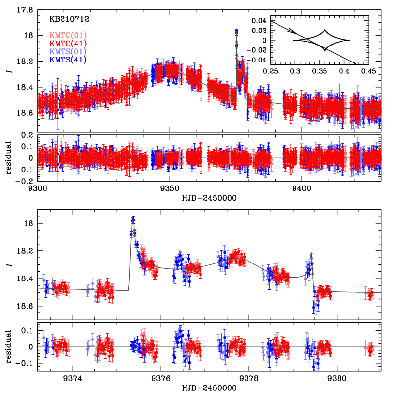
Figure 1: Light-curve data and models for KMT-2021-BLG-0712. Observations are color-coded by observatory and field, as indicated in the legend. Residuals to the model are shown for both the event as a whole (upper) and the anomaly region (lower) panels. The source trajectory relative to the (major-image planetary) caustic is shown in the inset.

Figure 1 shows an otherwise standard 1L1S light curve with Paczyński (1986) parameters $(t_{0},u_{0},t_{\rm E})=(9349.32,0.145,91\,{\rm day})$, punctuated by a 4.3-day double-horned profile, centered at $t_{\rm anom}=9377.35$. The double-horned profile is unusual in that it has a smooth bump in the middle, which is almost certainly generated by the source approaching an interior wall of the caustic.

3.2.1 Heuristic Analysis

These parameters imply $\tau_{\rm anom}=0.308$, $u_{\rm anom}=0.340$, and thus

$$\alpha=25^{\circ};\qquad s^{\dagger}_{+}=1.18.$$ (5)

Because the anomaly is clearly due to the source entering and leaving the caustic, we do not expect a degeneracy in $s$. Rather, we expect $s\simeq s^{\dagger}_{+}$.

3.2.2 Static Analysis

The grid search on the $(s,q)$ plane returns only one solution, whose refinement with all parameters set free is shown in Table 2. We find that $\alpha$ and $s$ are as expected, while $\log q=-3.3$ indicates a Saturn mass-ratio planet. The caustic entrance and exit are both well-covered, yielding a $\sim 8\%$ measurement of a relatively low value of $\rho=3.9\times 10^{-4}$. We will see in Section 4.1 that this implies a large value of $\theta_{\rm E}\sim 0.64\,{\rm mas}$, and so a relatively nearby lens $\pi_{\rm rel}\sim 0.05\,{\rm mas}/(M/M_{\odot})$ and thus a relatively large microlens parallax $\pi_{\rm E}\sim 0.08\,(\pi_{\rm rel}/0.05{\rm mas})$. Together with the relatively long timescale and the fact that the anomaly has three peaks (An & Gould, 2001), this encourages us to search for microlens parallax solutions, in spite of the relatively faint source, $I_{S,\rm KMTC01}\sim 21.6$.

3.2.3 Parallax Analysis

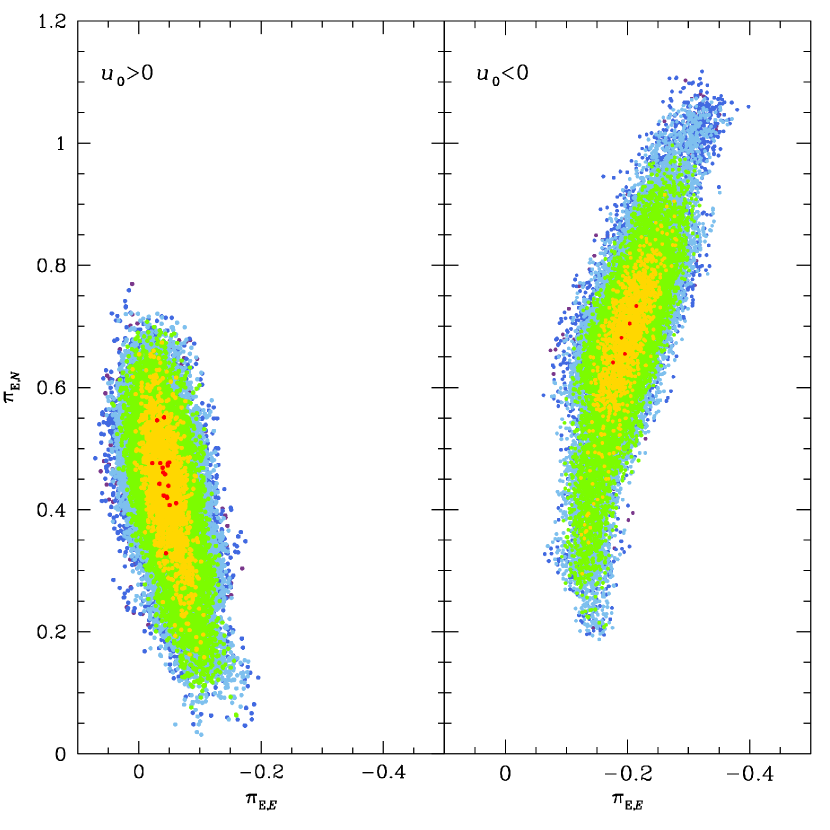
Figure 2: Scatter plot of MCMC trials in the ${\mbox{\boldmath$\pi$}}_{\rm E}=(\pi_{{\rm E},N},\pi_{{\rm E},E})$ plane for the $u_{0}>0$ (left) and $u_{0}<0$ (right) solutions of KMT-2021-BLG-0712. Points are colored (red, yellow, green, cyan, blue) if they are $\Delta\chi^{2}<(1,4,9,16,25)$ from the minimum.

As is almost always the case (except for some extremely long events), there are two parallax solutions, which are summarized in Table 2 and illustrated in Figure 2. As described in Section 3.1, we simultaneously fit for the first derivatives of the planet position due to its orbital motion $\gamma=[(ds/dt)/s,d\alpha/dt]$. While Table 2 gives ${\mbox{\boldmath$\pi$}}_{\rm E}$ in standard equatorial coordinates, it is also useful to present these solutions in terms of the principal axes of the error ellipses.

$$(\pi_{{\rm E},\parallel},\pi_{{\rm E},\perp},\psi)=(+0.123\pm 0.028,0.40\pm 0.11,280.4^{\circ})\qquad[u_{0}>0],$$ (6)

and

$$(\pi_{{\rm E},\parallel},\pi_{{\rm E},\perp},\psi)=(+0.033\pm 0.028,0.72\pm 0.14,256.4^{\circ})\qquad[u_{0}<0].$$ (7)

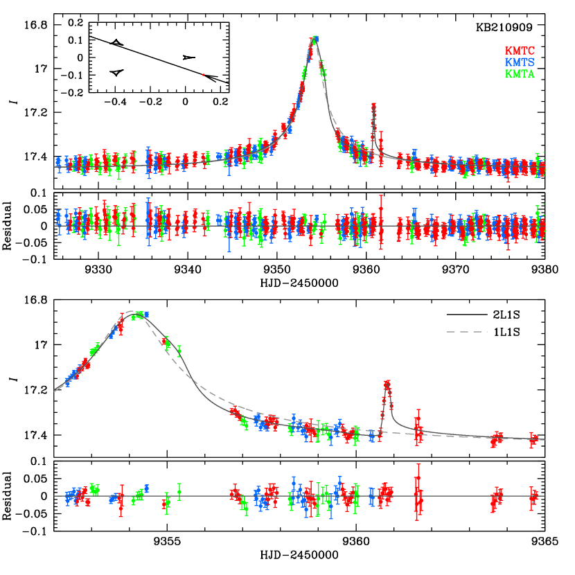
Figure 3: Light-curve data and models for KMT-2021-BLG-0909. Similar to Figure 1, except that the 1L1S model is also shown for comparison.

Here, $\pi_{{\rm E},\parallel}$ (so called because, for short events, it is approximately parallel to the projected position of the Sun) is the minor axis of the error ellipse, $\pi_{{\rm E},\perp}$ is the major axis, and $\psi$ is the angle of the minor axis, measured north through east. In line with the sign conventions of Figure 3 of Park et al. (2004) (keeping in mind that MOA-2003-BLG-037 peaked after opposition while KMT-2021-BLG-0712 peaked before opposition), $\pi_{{\rm E},\parallel}$ is approximately west and $\pi_{{\rm E},\perp}$ is approximately north. Note that the actual projected orientation of Earth relative to the Sun at the peak is $\psi_{\odot}=281.0^{\circ}$. Because the FWHM of the event, $\sqrt{12}u_{0}t_{\rm E}\sim 45\,$days, covers almost a radian of Earth’s orbit, the “short event” approximation (Smith et al., 2003; Gould, 2004; Park et al., 2004) is not expected to yield a precise characterization.

We find, from fitting the event (with the anomaly removed) to a point-lens model with parallax, that the presence of the anomaly reduces the axes of the error ellipses for the two solutions from (0.030:0.45) to (0.028:0.11) and from (0.032:0.39) to (0.028:0.14), in particular, reducing the aspect ratios by factors of 3.8 and 2.4 for the two cases. This confirms the important role of the relatively complex caustic features in improving the parallax measurement.

3.3 KMT-2021-BLG-0909

Figure 3 shows an otherwise approximately standard 1L1S light curve with parameters $(t_{0},u_{0},t_{\rm E})=(9354.1,0.060,16\,{\rm day})$, punctuated by a sharp bump, which erupts suddenly at 9360.65 and then peaks $\Delta t_{\rm rise}=4\,$hr later at $t_{\rm anom}=9360.82$. This is almost certainly a caustic entrance, although there is no obvious caustic exit.

3.3.1 Heuristic Analysis

These parameters imply $\tau_{\rm anom}=0.420$, $u_{\rm anom}=0.424$, and thus

$$\alpha=188.1^{\circ};\qquad s^{\dagger}_{+}=1.23.\qquad s^{\dagger}_{-}=0.81.$$ (8)

Note that because the nature of the caustic entrance is unclear, we report both $s^{\dagger}_{+}$ and $s^{\dagger}_{-}$. Moreover, because $u_{\rm anom}\sim 0.4$ is large, this is a planetary caustic crossing, so we do not expect a degeneracy in $s$. Rather, for a major-image caustic, we expect $s\simeq s^{\dagger}_{+}$, while for a minor-image caustic, we expect a less precise $s\sim s^{\dagger}_{-}$ because the caustic would not lie on the binary axis.

3.3.2 Static Analysis

The grid search returns only one solution, whose refinement is described by the parameters given in Table 3. The heuristic estimate of $\alpha$ proves to be too small by a factor of two relative to the binary axis, i.e., $\alpha-180^{\circ}=8.1^{\circ}$ versus $18.9^{\circ}$. This is because the source crosses the binary axis about half way between the central and planetary caustics, rather than at the planetary caustic. See Figure 3. This, in turn, is partly due to the fact that the planet is relatively massive, $\log q=-2.50$, for which the caustics are offset from the axis by $\eta_{c,-}=2[q(s^{-2}-1)]^{1/2}\rightarrow 0.078$ (Han, 2006). See Figure 3. Because the caustic entrance is well-covered by KMTC data, the normalized source radius, $\rho$, is determined to better than 10%. Given the short Einstein timescale $t_{\rm E}=16\,$day and the faintness of the source, we do not attempt a measurement of ${\mbox{\boldmath$\pi$}}_{\rm E}$.

3.4 KMT-2021-BLG-2478

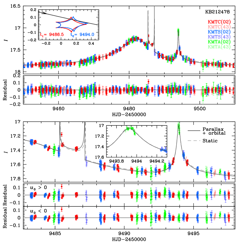
Figure 4: Light-curve data and models for KMT-2021-BLG-2478. Similar to Figure 1 except that the source-trajectory inset shows the caustic structure at two epochs and both the static and parallax models are indicated. In addition there is an inset in the lower panel that highlight the KMTA coverage of the peak of the “spike”.

Figure 4 shows an approximately standard 1L1S light curve with parameters $(t_{0},u_{0},t_{\rm E})=(9482.2,0.08,41\,{\rm day})$, but with two major features superposed: a poorly sampled caustic feature, centered at $\sim 9486$, lasting 1.5–2 days, and a roughly 2-day, roughly symmetric spike, peaking at 9493.9. The sparse coverage is primarily due to the fact that these anomalies occurred near the end of the microlensing season, when the field was visible only about 3 hours per night from each site, and partly due to episodes of adverse weather.

The first (i.e., caustic) structure implies that there must be a second lens. If the system is not more complicated than this, i.e., it is 2L1S, then the presence of two anomalies at $\tau_{1}\sim+0.09$ and $\tau_{2}\sim+0.29$ after peak almost certainly implies a very large resonant caustic. In principle, however, such multiple anomalies might require more complex systems, such as 3L1S.

3.4.1 Heuristic Analysis

Within the 2L1S framework, $t_{\rm anom}=9493.9$, i.e., $\tau_{\rm anom}=\tau_{2}=0.29$, and $u_{\rm anom}=0.30$, so

$$\alpha=14.9^{\circ};\qquad s^{\dagger}_{+}=1.16.$$ (9)

3.4.2 Static Analysis

The grid search yields only one solution, whose refined parameters are given in Table 4. Note that while the heuristic $\alpha$ prediction was approximately correct, the heuristic $s^{\dagger}_{+}$ (combined with $s=1.058$ from Table 4), predicts a second solution at $s_{\rm inner}=(s^{\dagger}_{+})^{2}/s_{\rm outer}=1.27$. Such solutions can generate a cusp-approach spike as the source passes over the ridge between the central and planetary caustics, but the central caustic is not large enough to induce the first caustic anomaly that is seen in the light curve. Hence, there is no degeneracy.

As with KMT-2021-BLG-0909, this planet has a super-Jovian mass ratio.

The Markov Chain Monte Carlo (MCMC) constraints on $\rho$ are not adequately summarized by the median and 68 percentile format of Table 4. The main takeaway would be that, at the $1\,\sigma$ level, $\rho<1\times 10^{-4}$. In Section 4.3, we will show that $\theta_{*}\sim 0.5\,\mu{\rm as}$. Hence, this limit would imply $\theta_{\rm E}>5\,{\rm mas}$, which would be quite extraordinary. We defer investigation of the reliability of such limits to Section 3.4.3, but for the moment we simply note that we must at least consider the possibility of very large $\theta_{\rm E}=\sqrt{\kappa M\pi_{\rm rel}}$ and so very nearby and/or very massive lenses. The former would imply a large, hence potentially measurable microlens parallax $\pi_{\rm E}$. As mentioned in Section 3.2.2, the complex caustic structure, spanning a significant fraction of $t_{\rm E}$, greatly enhances the prospects for making such a measurement.

3.4.3 Parallax Analysis

Including ${\mbox{\boldmath$\pi$}}_{\rm E}$ and $\gamma$ improves the fit by $\Delta\chi^{2}=146$, with the $u_{0}>0$ and $u_{0}<0$ being almost perfectly degenerate. See Table 4. The most important aspect of these fits is that $\pi_{\rm E}\simeq\pi_{{\rm E},E}=0.52\pm 0.07$ (because $|\pi_{{\rm E},E}|\gg|\pi_{{\rm E},N}|$) is indeed large.

However, these solutions imply that the $\rho$ measurement requires closer examination. In particular, the $1\,\sigma$ limit remains similar, which, if accepted at face value, would imply $M>1.2\,M_{\odot}$ and $D_{L}<0.4\,{\rm kpc}$. Clearly, such a lens would be so bright, $I_{L}\lesssim 12$, as to prevent microlensing observations in its neighborhood, unless it were a black hole or neutron star.

Hence, we must investigate the origins of the $\rho$ limit in the light curve and also consider the extent to which it can be relaxed within acceptable statistical limits.

The constraints on $\rho$ come entirely from the curvature in the KMTA data during the spike, which drop by $\sim 0.1\,$mag over the course of $\delta t\sim 0.25\,$hr. Because the source is crossing the ridge extending from the caustic at a steep angle $\alpha^{\prime}=\alpha+(d\alpha/dt)\Delta t_{2}=16^{\circ}$ (where $\Delta t_{2}=11.1\,$day), the intrinsic timescale of this feature is foreshortened to $\delta t\sin\alpha^{\prime}=0.07\,$hr, which is driving the extremely short $t_{*}<0.08\,$hr in Table 4.

These late-season, end-of-night data were taken at high (for KMT) airmass of $\sim 1.9$, which raises the possibility of a spurious decline in flux due to deteriorating seeing or other effects. Indeed, we find that the structure of the KMTA peak is remarkably well anti-correlated with seeing over the whole night. However, after conducting several tests, we find no evidence for flux-seeing correlations in other parts of the KMTA light curve. Thus, we cannot simply reject this light-curve structure as seeing-induced.

Next, we investigate in more detail the statistical limits on $\rho$ under the assumption that systematics play no role. We carry out fits including ${\mbox{\boldmath$\pi$}}_{\rm E}$ and $\gamma$ with $\rho$ fixed at various values. We find that values of $\rho=(1,2,4,8)\times 10^{-4}$ are disfavored at $\Delta\chi^{2}=(1.4,3.2,7.4,19.4)$. Thus, we regard $\rho=3\times 10^{-4}$ as marginally acceptable even assuming Gaussian statistics. If we further take account of possible systematics from end-of-night data taken at high airmass, even if we cannot identify a specific physical cause, the constraints become weaker. Therefore, we will treat the $\rho$ limits cautiously when we investigate the physical nature of the system in Section 5.3.

3.5 KMT-2021-BLG-1105

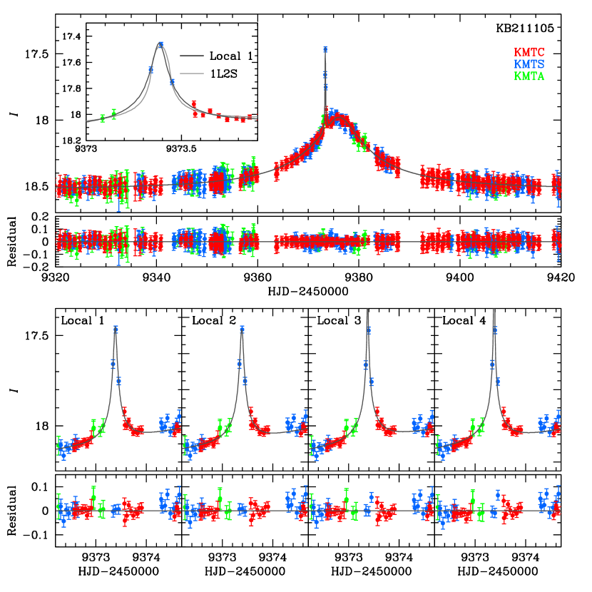
Figure 5: Light-curve data and models for KMT-2021-BLG-1105. Similar to Figure 1, except that the anomaly region is shown in separate panels for the four solutions at the bottom, while the inset at the top compares the 1L2S solution to the Local-1 2L1S solution. In addition, because there are four caustic topologies, these are shown separately in Figure 6.

Figure 5 shows an otherwise standard 1L1S light curve with parameters $(t_{0},u_{0},t_{\rm E})=(9375.8,0.11,35\,{\rm day})$, punctuated by a sharp spike at $t_{\rm anom}=9373.4$, i.e., 2.3 days before peak.

3.5.1 Heuristic Analysis

These parameters imply $\tau_{\rm anom}=0.07$, $u_{\rm anom}=0.13$, and so

$$\alpha=122^{\circ};\qquad s^{\dagger}_{+}=1.067.$$ (10)

3.5.2 Static Analysis

Somewhat surprisingly, the grid search returns 6 local minima. After refinement, we reject two of these because they have high $\Delta\chi^{2}=69$ and 109 and, moreover, have poor fits by eye. However, we briefly note that both have relatively high mass ratios $\log q\sim-1.75$ and for both, the spike arises from an off-axis cusp approach to a resonant caustic. While these models are certainly not correct, they emphasize the importance of making a systematic search of parameter space because the overall appearance of the models is not qualitatively different from the observed light curve.

The remaining four models are shown in Figure 5, with the corresponding geometries shown in Figure 6, while their refined parameters are given in Table 5. Locals 1 and 2 constitute an inner/outer degeneracy with $s^{\dagger}=1.068$, while Locals 3 and 4 constitute a second inner/outer degeneracy with $s^{\dagger}=1.066$, both in excellent agreement with Equation (10). This again emphasizes the importance of a systematic search. Because Locals 3 and 4 are each disfavored by $\Delta\chi^{2}>10$, we consider that these solutions are excluded. Nevertheless, it is notable that these two pairs of solutions differ in $q$ by more than a factor of 2.

This is another super-Jovian mass-ratio planet, $\log q=-2.7$.

We note that while $\rho$ is not measured, the constraint, $\rho<0.0013$, at $2.5\,\sigma$, corresponding to $t_{*}<1.1\,$hr, is strong enough to play a significant role. That is, in Section 4.4, we will show that $\theta_{*}=0.5\,\mu{\rm as}$, implying $\mu_{\rm rel}=\theta_{*}/t_{*}>4\,{\rm mas}\,{\rm yr}^{-1}$, which excludes a significant part of proper-motion parameter space. Hence, when we incorporate the $\rho$ constraint to estimate the physical parameters of the system in Section 5.4, we apply the full $\chi^{2}(\rho)$ envelope function, rather than a simple limit. For the moment, we simply note that even the $1\,\sigma$ “limit” corresponds to $\mu_{\rm rel}>6.5\,{\rm mas}\,{\rm yr}^{-1}$, and so still leaves a substantial range of values that are well-populated by Galactic models. This fact will become relevant in Section 3.5.3.

Due to the faintness of the source and the lack of complex anomaly structures, we do not attempt a parallax analysis.

3.5.3 Binary-Source Analysis

As with all bump-like anomalies that lack complex or caustic-crossing features, we must check whether the anomaly can be produced by a second source (1L2S) rather than a second lens (2L1S). The results are shown in Table 6.

There are two main features to note about this solution. First, while the $\chi^{2}$ difference, $\Delta\chi^{2}=\chi^{2}({\rm 1L2S})-\chi^{2}({\rm 2L1S})=5.5$, favors the 2L1S solution, it is not large enough, by itself, to definitively rule out the 1L2S solution.

Second, the value of the second-source self-crossing time, $t_{*,2}=1.28\,$hr, is well-measured in this model (contrary to 2L1S), with just a 5% error. At first sight, this value appears to be very “typical” of historic measurements of $t_{*}$ for dwarf-star sources in microlensing events. However, in this instance, the source is about 100 times fainter than typical cases, $I_{S,2}=26.3$. We will show in Section 4.4 that this implies $\theta_{*,2}=0.169\,\mu{\rm as}$ and thus $\mu_{\rm rel}=\theta_{*,2}/t_{*,2}=1.16\,{\rm mas}\,{\rm yr}^{-1}$. Only a fraction of $p<(\mu_{\rm rel}/\sigma_{\mu})^{3}/6\sqrt{\pi}\rightarrow 0.006$ microlensing events will have such low proper motions (e.g., Gould et al. 2021a, 2022b). Here, we have approximated the bulge proper-motion distribution as an isotropic Gaussian, with $\sigma_{\mu}=2.9\,{\rm mas}\,{\rm yr}^{-1}$. For example, in a systematic study of 30 1L1S events with finite-source effects (thus permitting $\mu_{\rm rel}$ measurements), which was sensitive to $\mu_{\rm rel}\geq 1.0\,{\rm mas}\,{\rm yr}^{-1}$, Gould et al. (2022a) found that the slowest (KMT-2019-BLG-0527) had $\mu_{\rm rel}=1.45\,{\rm mas}\,{\rm yr}^{-1}$, i.e., $\sigma_{\mu}/2$. See their Figure 5. Thus, the combination of the $\Delta\chi^{2}$ preference discussed above, together with this kinematic argument, overwhelmingly favors the 2L1S (i.e., planetary) interpretation.

For completeness, we remark that because the second source would be very red, the 1L2S model predicts that the bump-anomaly would be much less pronounced in the $V$ band than the $I$ band. See, e.g., Hwang et al. (2019) for a practical example. Unfortunately, however, there are no $V$-band data during the anomaly.

Because the interpretation of the event rests heavily on the kinematic argument, we must also consider the possibility that this argument can be evaded (at some cost in $\chi^{2}$) by solutions with much smaller $\rho$. We first check that the $1\,\sigma$ error bar on $\rho_{2}$ shown in Table 6 is actually representative of the $\chi^{2}$ surface out to $3\,\sigma$ by fixing $\rho_{2}$ at various values. We find that it is. See Table 6 for an example. Next, we search for solutions that are away from this local minimum by enforcing $\rho_{2}=0$. We find that there is such a solution, but it is disfavored by $\Delta\chi^{2}=13.4$. See Table 6. Thus, while this solution avoids the proper-motion constraint, it increases the total $\chi^{2}$ difference to $\Delta\chi^{2}=\chi^{2}({\rm 1L2S})-\chi^{2}({\rm 2L1S})=19$. This would be high enough to decisively reject 1L2S were we to adopt the low-$\rho_{2}$ solution.

Moreover, there is an additional statistical argument against the 1L2S solution, From the Local-1 panel of Figure 6, it is clear that there is a range of “$x$”, i.e., $u_{x}$, of about 0.15 Einstein radii that would generate a qualitatively similar non-caustic-crossing bump. However, the 1L2S solution requires the source to cross the face of the second source, which has a probability of $p=2\rho_{2}\simeq 0.003$, i.e., about 50 times smaller. To fully evaluate this relative probability, we would have to consider the relative probabilities of the presence of lens planetary companion, compared to a source M-dwarf companion, which we do not attempt here because it is unnecessary to make the basic argument. Nevertheless, it is clear that the 1L2S solution requires some fine tuning.

While we cannot absolutely rule out the 1L2S solution, the formal probability that it is correct is about $p\sim 4\times 10^{-4}$. Hence, this planet should be accepted as genuine. We note that its reality can be definitively tested at first adaptive optics (AO) light on next generation (30m) telescopes, roughly in 2030, i.e., $\Delta t=9\,$yr after the event. If, as anticipated, the 2L1S model is correct, then the source and lens will be separated by $\Delta\theta=\mu_{\rm rel}\Delta t\gtrsim 36\,{\rm mas}$, so they will be easily resolved. On the other hand, if the 1L2S model were correct, then the separation would be $\Delta\theta\sim 9\,{\rm mas}\,{\rm yr}^{-1}$, which would probably be too small to resolve, but even if resolved would provide a measurement that was consistent with 1L2S but not with 2L1S.

Before leaving the issue of 1L2S models, we note that as a matter of “due diligence”, we explored 1L2S models in which finite-source effects were permitted for both the primary and secondary sources, even though such effects are extremely unlikely for the primary, a priori, because $t_{\rm eff}\equiv u_{0}t_{\rm E}\sim 4\,$days is extremely long relative to the typical self-crossing time of dwarf stars, $t_{*}\sim 1\,$hr. Surprisingly, we did indeed find such solutions with $\Delta\chi^{2}\sim-6$ relative to the solution reported in Table 6 (so, comparable $\chi^{2}$ to the 2L1S solution). However, these had $(\rho_{1},\rho_{2})\simeq(0.2,0.002)$, which would imply grossly inconsistent estimates for $\theta_{\rm E}=\theta_{*}/\rho$ of $2.5\,\mu{\rm as}$ versus $85\,\mu{\rm as}$. Hence, it is unphysical. The $\chi^{2}$ improvement could be a purely statistical fluctuation ($p=0.05$) or it could be due to low level systematics in the photometry. In any case, we reject this solution.

Finally, we remark that this event was included in the present study only because our “mass production” project aims to document all 2021 events with viable planetary solutions, in the spirit pioneered by Gould et al. (2022b) and Jung et al. (2022) for 2018 events, irrespective of whether such planetary solutions are decisively preferred. Our initial assessment, based on detailed modeling of TLC reductions, was that its interpretation was ambiguous, and thus it would not enter planetary catalogs. It was only in the course of comprehensively evaluating all the evidence that we concluded that the planetary solution is decisively favored.

4 Source Properties

Our evaluation of the source properties exactly follows the goals and procedures of Paper I. In this introduction, we repeat only the most essential descriptions from Section 4 of that work, in particular (as in Section 3.1) documenting all notation.

We analyze the color-magnitude diagram (CMD) of each event, primarily to measure $\theta_{*}$ and so to determine

$$\theta_{\rm E}={\theta_{*}\over\rho};\ \qquad\mu_{\rm rel}={\theta_{\rm E}\over t_{\rm E}}.$$ (11)

We follow the method of Yoo et al. (2004). We first find the offset of the source from the red clump

$$\Delta[(V-I),I]=[(V-I),I]_{S}-[(V-I),I]_{\rm cl}.$$ (12)

We adopt $(V-I)_{\rm cl,0}=1.06$ from Bensby et al. (2013) and evaluate $I_{\rm cl,0}$ from Table 1 of Nataf et al. (2013), based on the Galactic longitude of the event, which yields the dereddened color and magnitude of the source,

$$[(V-I),I]_{S,0}=[(V-I),I]_{\rm cl,0}+\Delta[(V-I),I].$$ (13)

Next, we transform from $V/I$ to $V/K$ using the $VIK$ color-color relations of Bessell & Brett (1988), and we apply the color/surface-brightness relations of Kervella et al. (2004) to obtain $\theta_{*}$. After propagating the measurement errors, we add 5% to the error in quadrature to take account of systematic errors due to the method as a whole.

To obtain $[(V-I),I]_{S}$, we always begin with pyDIA reductions (Albrow, 2017), which put the light curve and field-star photometry on the same system. With one exception (see below), we determine $(V-I)_{S}$ by regression of the $V$-band data on the $I$-band data, and we determine $I_{S}$ by regression of the $I$-band data on the best-fit model. For 2 of the 4 events analyzed in this paper, there is calibrated OGLE-III field-star photometry (Szymański et al., 2011). For these 2 cases, we transform $[(V-I),I]_{S}$ to the OGLE-III system. For the 2 remaining cases, we work in the instrumental KMT pyDIA system.

For KMT-2021-BLG-0909, the source is too faint in the $V$ band to measure the source color from the light curve. We therefore employ a different technique, as described in Section 4.2.

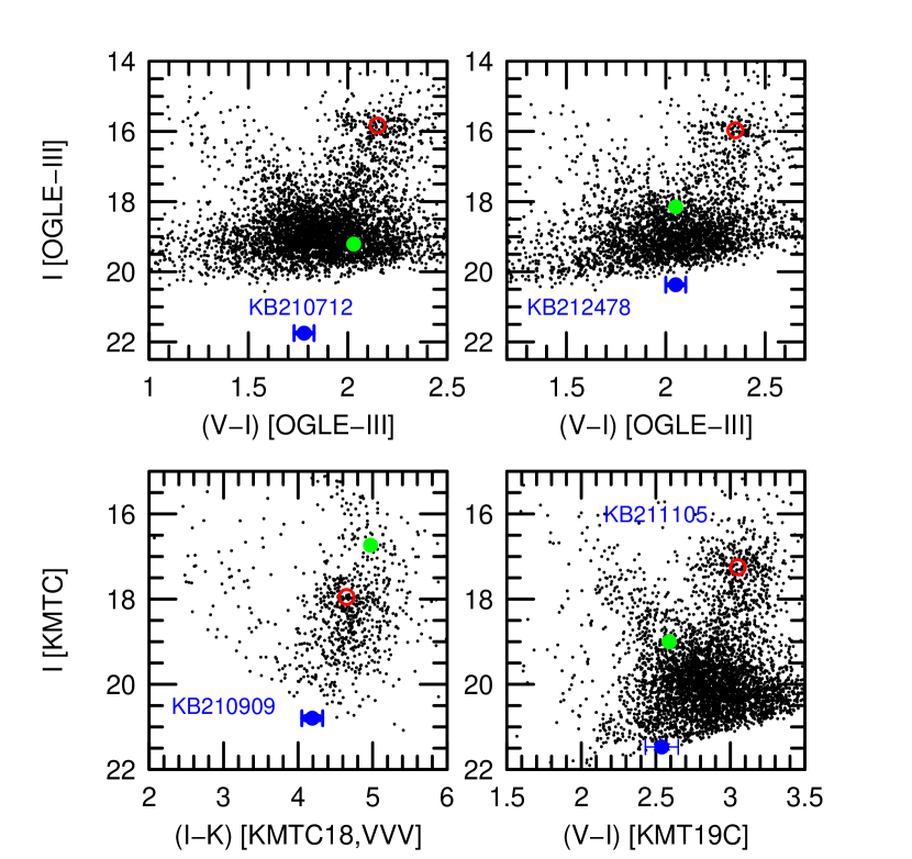
Figure 7: CMDs for each of the four planets reported here. The source positions (blue) and clump-giant centroids (red) are shown for all events. Where relevant, the blended light is shown in green.

The CMDs are shown in Figure 7.

The elements of these calculations are summarized in Table 7. In all cases, the source flux is that of the best solution. Under the assumption of fixed source color, $\theta_{*}$ scales as $10^{-\Delta I_{S}/5}$ for the other solutions, where $\Delta I_{S}$ is the difference in source magnitudes, as given in the Tables of Section 3. The inferred values (or limits upon) $\theta_{\rm E}$, and $\mu_{\rm rel}$ are given in the individual events subsections below, where we also discuss other issues, when relevant.

4.1 KMT-2021-BLG-0712

There are two issues related to the source that require some care for this event. First, the source color shown in Table 7, $(V-I)_{S,0}=0.69\pm 0.06$, is unusually blue given that the source lies $\Delta I=5.9$ magnitudes below the clump. If the source were a typical bulge star of this brightness, we would expect $(V-I)_{S,0}\sim 1.1$, based on Hubble Space Telescope images of Baade’s Window taken by Holtzman et al. (1998). Logically, there are three possibilities: our color measurement is incorrect; the source lies well behind the bulge and thus is much more luminous (and so bluer) than a bulge star of similar brightness; or the source is atypical, e.g., has much lower metallicity than typical bulge stars. The first of these explanations is the only one of direct concern here: if the color and magnitude of the source are correctly measured, regardless of the exact cause of it being so blue, then the derived $\theta_{*}$ will also be correct.

We therefore check the color determination as follows: The color and magnitude reported in Table 7 are based on the KMTC41 data set. We repeat the calculation using the KMTC01 data set, which is composed of a completely independent series of observations. While these observations are made with the same (KMTC) telescope, the observational times are different, and the positions on the focal plane are offset by $8^{\prime}$. Yet, the best-fit color is the same to within 0.01 mag. Neither of the other two explanations appear likely a priori. To be sufficiently more luminous to account for the color discrepancy, the source should be roughly a factor of 2 more distant than the bulge, which would place it almost 1 kpc below the Galactic plane. While there are certainly some stars at this height and this Galactocentric radius (i.e., similar to that of the Sun), they are relatively rare. Extremely metal-poor stars in the bulge are likewise rare.

Despite the low prior likelihood of either of these two options, they are not unphysical, and hence we adopt the measured color, and so the value of $\theta_{*}=0.255\,\mu{\rm as}$ given in Table 7, and we thereby derive,

$$\theta_{\rm E}=0.604\pm 0.095\,{\rm mas};\qquad\mu_{\rm rel}=2.19\pm 0.34\,{\rm mas}\,{\rm yr}^{-1},\qquad(u_{0}<0)$$ (14)

and

$$\theta_{\rm E}=0.636\pm 0.091\,{\rm mas};\qquad\mu_{\rm rel}=2.62\pm 0.37\,{\rm mas}\,{\rm yr}^{-1},\qquad(u_{0}>0)$$ (15)

The second issue that requires some care is the location of the blend relative to the source. If these were closely aligned, it would argue for the blend being associated with the event, either being the lens itself or a companion to the lens or the source.

In the KMTC41 pyDIA analysis, the baseline object appears to lie $\Delta{\mbox{\boldmath$\theta$}}(N,E)=(170,145)\,{\rm mas}$ northeast of the source. The issue that requires care is that there is another, slightly brighter star that lies $1^{\prime\prime}$ northwest of the baseline object, which could in principle corrupt the astrometry of the baseline object. (The position of the source is determined from difference images, for which no such issues arise.)  We conduct two tests. First, we repeat the analysis using the KMTC01 observations and find almost exactly the same result. Second, we find, after transforming coordinates to the OGLE-III system, that the offset is qualitatively similar: $\Delta{\mbox{\boldmath$\theta$}}(N,E)=(80,250)\,{\rm mas}$. Note that because the epoch of the OGLE-III data is 15 years earlier, we expect offsets of order 50 mas in each direction, in addition to normal measurement errors. The blend is 0.12 mag bluer and and 3.38 mag fainter than the clump (see Figure 7), and it is therefore likely to be a bulge subgiant. We conclude that it is most likely not related to the event. The lens must be fainter than the blend, but because the two are separated by just 220 mas, we cannot place more stringent constraints on the lens light than this.

4.2 KMT-2021-BLG-0909

Due to high extinction, $A_{I}\sim 4$, the source is too faint in the $V$ band to measure the source color from the light curve. In such cases, one generally estimates the source color based on its offset in the $I$ band from the centroid of the red clump. As often happens for such heavily reddened fields, it is difficult to precisely locate the red clump on the pyDIA (or, when available, OGLE-III) CMD because even red clump stars are near or below the measurement threshold in the $V$ band. In the present case, we find that red clump is detectable on the pyDIA CMD, but its centroid cannot be reliably determined because the lower part of the clump merges into the background noise of the diagram.

Therefore, we measure the clump centroid on an $[(I-K),I]$ CMD, which we construct by matching pyDIA $I$-band photometry with $K$-band photometry from the VVV catalog (Minniti et al., 2017). See Figure 7. To estimate the color, we first find the offset from the clump $\Delta I=I_{S}-I_{\rm cl}=2.85\pm 0.08$. See Table 7. If the source were exactly at the mean distance of the clump, it would therefore have an absolute magnitude, $M_{I}=2.73$. In fact, it is more likely to be toward the back of the bulge (because it must be behind the lens), so a plausible range of possibilities is $2.2\lesssim M_{I}\lesssim 2.9$. In this range, the source could be almost anywhere along the turnoff/subgiant branch. To account for this, we adopt a uniform distribution, $0.60<(V-I)_{S,0}<1.00$, which we summarize as a $1\,\sigma$ range of $(V-I)_{S,0}=0.80\pm 0.12$. This source position is illustrated in Figure 7 by transforming from $(V-I)$ to $(I-K)$ using the relations of Bessell & Brett (1988). These values lead to estimates of

$$\theta_{\rm E}=0.362\pm 0.049\,{\rm mas};\qquad\mu_{\rm rel}=8.24\pm 1.11\,{\rm mas}\,{\rm yr}^{-1}.$$ (16)

Also shown in the CMD is the position of the blended light, which is a bright giant that is more than 1 mag above the clump. We find that this star is displaced by $0.73^{\prime\prime}$ from the source toward the southwest. This bright star is almost certainly not associated with the event, but it prevents us from placing any useful limits on the lens light.

For completeness, we note that the coordinates shown for this event in Table 1 are, as usual, those of the nearest catalog star, namely the bright giant just discussed. However, these differ from the coordinates shown on the KMT webpage, which are about $1.5^{\prime\prime}$ yet farther south. When the event was originally triggered by AlertFinder (Kim et al., 2018b), it was identified with this more southerly catalog star. One day later, it was again triggered, this time by the closer (bright) catalog star, but our standard procedures enforce maintaining the coordinates of the original announcement on the web page to avoid confusion.

4.3 KMT-2021-BLG-2478

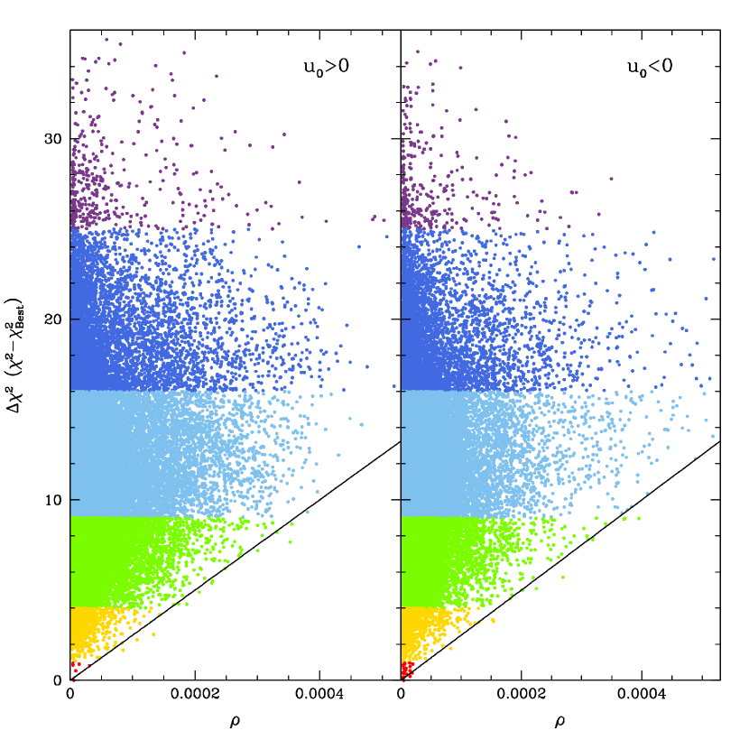
Figure 8: Envelope function (solid curve) of $\Delta\chi^{2}(\rho)$ derived from the lower limit of MCMC trials (colored points) for KMT-2021-BLG-2478.

The source star, whose parameters are given in Table 7 and whose CMD position is shown in Figure 7, lies 4.4 mag below the clump and is about $0.07\pm 0.06$ mag redder than the Sun. That is, it is a bulge middle-G dwarf. Unfortunately, as discussed in Section 3.4, we have only a $\chi^{2}$-envelope constraint on $\rho$, rather than a measurement. See Figure 8. For the present, we therefore present the estimates of $\theta_{\rm E}$ and $\mu_{\rm rel}$ scaled to that section’s “marginally acceptable limit” (assuming Gaussian errors),

$$\theta_{\rm E}={3\times 10^{-4}\over\rho}(1.78\pm 0.014)\,{\rm mas}\qquad\mu_{\rm rel}={3\times 10^{-4}\over\rho}(19.3\pm 1.6)\,{\rm mas}\,{\rm yr}^{-1}.$$ (17)

The high value of $\mu_{\rm rel}$ is particularly unexpected. If there were no reasons to suspect that this might be due to systematics in end-of-night data, it would have to be “cautiously accepted”. In our actual case, it invites serious doubt on the reliability of the $\rho$ measurement.

A more robust kinematic constraint comes from $\pi_{\rm E}=0.53\pm 0.07$, which yields a projected velocity of

$$\tilde{v}\equiv{{\rm au}\over\pi_{\rm E}t_{\rm E}}=97\pm 13\,{\rm km}\,{\rm s}^{-1}.$$ (18)

From this, one may make a rough estimate of the lens distance (e.g., Han & Gould 1995), $\pi_{\rm rel}=(v_{\rm rot}/\tilde{v})({\rm au}/R_{0})\rightarrow 0.30\,{\rm mas}$, i.e., $D_{L}\sim 2.4\,{\rm kpc}$, where $v_{\rm rot}\simeq 235\,{\rm km}\,{\rm s}^{-1}$ is the rotation speed of the Galaxy and $R_{0}\simeq 8\,{\rm kpc}$ is the Galactocentric distance. Because this rough estimate is in only mild tension with the “surprising” result in Equation (17), we will, in Section 5.3, consider and compare results that both include and remove the constraints on $\rho$.

Figure 7 shows the location of the blended light, which is 2.2 mag brighter than the source and of similar color. We find that the source is displaced from the baseline object by $\Delta\theta=220\,{\rm mas}$ to the southeast. It is consistent with being a bulge turnoff/subgiant star and thus could in principle be a companion to the source, but there is no strong evidence in favor of this hypothesis. In Section 5.3, we will impose the constraint on lens light: $I_{L}>I_{B}$. This constraint will further support the caution regarding the $\rho$ measurement. For example, if the lens has $\pi_{\rm rel}=0.30\,{\rm mas}$ as crudely estimated above from the kinematic argument (which ignores the $\rho$ constraint), then $M\simeq 0.12\,M_{\odot}$ and $D_{L}\simeq 2.4\,{\rm kpc}$, which would be far fainter than this limit on lens light. However, if we were to accept the “marginally acceptable limit” on $\rho$, then $M>0.4\,M_{\odot}$ and $D_{L}<1\,{\rm kpc}$, which would imply that the lens light exceeds this limit, unless the lens were a remnant.

4.4 KMT-2021-BLG-1105

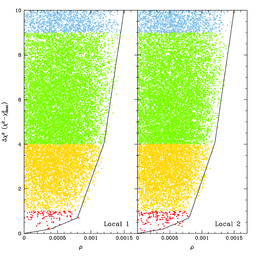
Figure 9: Envelope function (solid curve) of $\Delta\chi^{2}(\rho)$ derived from the lower limit of MCMC trials (colored points) for KMT-2021-BLG-1105.

As shown in Table 7, the source star lies 4.24 mag below the clump and is measured to have $(V-I)_{S,0}=0.51\pm 0.09$. This is unexpectedly blue, although it is within $1\,\sigma$ of a plausible value for a relatively metal-poor turn-off star. We attempt to check this measurement using KMTS data. However, these have too few magnified $V$-band points for a reliable measurement. We adopt the orientation that our normal error estimates adequately cover the measurement uncertainty. As discussed in Section 3.5, we obtain only a $\chi^{2}(\rho)$ envelope function which we will incorporate into the Bayesian analysis in Section 5.4. See Figure 9. Hence, the $\theta_{*}$ determination in Table 7 does not lead to unambiguous estimates of $\theta_{\rm E}$ and $\mu_{\rm rel}$. These can be fully investigated only in the context of the Bayesian analysis. For the moment, we express them in parametric form,

$$\theta_{\rm E}={8.2\times 10^{-4}\over\rho}\times(0.59\pm 0.07)\,{\rm mas};\qquad\mu_{\rm rel}={8.2\times 10^{-4}\over\rho}\times(6.1\pm 0.7)\,{\rm mas}\,{\rm yr}^{-1},$$ (19)

where the prefactor has values $\simeq(1,0.71,0.57)$ at $\Delta\chi^{2}=(1,4,9)$ of the envelope function. Thus, in contrast to many cases that lack a clear $\rho$ measurement, the $\rho$ constraint will play a significant role.

As also discussed in Section 3.5, evaluating the angular radius of the second source in the 1L2S solution, $\theta_{*,2}$, is critically important to the kinematic argument against this solution. We present a new method for doing so, which is particularly adapted to mid-late M dwarfs, for which it may be very difficult to make the color measurements that are needed for the traditional (Yoo et al., 2004) method. The first step is to note, from Tables 5 and 6, that this second source is 5.11 mag fainter than the source in the Local-1 2L1S model, which (from Table 7) is 4.22 mag fainter than the clump. That is, the second source is $9.33\pm 0.11$ mag fainter than the clump, where the error is the quadrature sum of the errors in $I_{S,2}$ (Table 6) and $I_{\rm cl}$ (Table 7). We adopt $I_{\rm cl,0}=14.37$ and $M_{I,\rm cl}=-0.12$.

We do not know, a priori, the exact distance of the source system along the line of sight. As noted above, the primary source appears to be a bulge turnoff star and so could in principle be anywhere in the bulge. We will consider below the full range of distances, but for the moment we adopt a fiducial distance modulus ${\rm Dmod}_{\rm fid}=14.37-(-0.12)+0.2=14.69$, i.e., 0.2 mag behind the clump centroid.

Next, we evaluate the second source radius under the assumption that it lies exactly at this distance, and we initially ignore the error in its flux measurement. That is, we initially assume that it has an absolute magnitude $M_{I,2}=9.33+(-0.12)-0.20=9.01$. Using the mass-luminosity relations of Benedict et al. (2016) in $V$ and $K$, together with the $VIK$ color-color relations of Bessell & Brett (1988), we find that the mass of the putative second source would be $M_{S,2}=0.314\,M_{\odot}$. We then adopt the M-dwarf mass-radius relation $(R/R_{\odot})=(M/M_{\odot})$ from Figure 7 of Parsons et al. (2018), and so obtain $R_{2}=0.314\,R_{\odot}$ and thus $\theta_{*,2}=0.169\,\mu{\rm as}$.

We now take account of the fact that the source system could be at other distance moduli in the bulge. For example, if it were at 0.1 mag larger Dmod, then it would likewise be 0.1 mag more luminous, and so would have correspondingly larger mass (and radius), but the impact of this larger physical size on $\theta_{*,2}$ would be countered by the larger distance of the system. Applying the above arguments to arbitrary distances (within the bulge), we find, $dM_{I}/d\ln M=-2.430$ and so (after a few steps),

$$\theta_{*,2}=0.169\,\mu{\rm as}\times 10^{-0.0213\,\Delta{\rm Dmod}},$$ (20)

where $\Delta{\rm Dmod}$ is the difference between the true distance modulus and the fiducial one adopted above. Stated alternatively, $\theta_{*,2}\propto D_{S}^{0.046}$. Thus, for example, if we adopt $\Delta{\rm Dmod}=0\pm 0.3$, then (still not taking account of the measurement error of $\sigma(I_{s,2})=0.11$), we find $\theta_{*,2}=0.169\pm 0.003\,\mu{\rm as}$. The main error then comes from this measurement error, $\sigma(\ln\theta_{*})=0.11/2.43=0.045$. This leads to $\mu_{\rm rel}=1.16\pm 0.08\,{\rm mas}\,{\rm yr}^{-1}$, which we argued in Section 3.5.3 is highly unlikely.

Finally, the blended light lies on the foreground main sequence of the CMD in Figure 7. In principle, it might therefore be the lens or a companion to lens. We therefore carefully investigate the offset between the magnified source and the baseline object $\Delta{\mbox{\boldmath$\theta$}}(N,E)={\mbox{\boldmath$\theta$}}_{\rm base}-{\mbox{\boldmath$\theta$}}_{S}$. We make four measurements by applying two independent algorithms (pyDIA and pySIS) to two independent data sets (KMTC and KMTS). The best-fit values of the measurements are (in mas), $\Delta{\mbox{\boldmath$\theta$}}_{\rm KMTC,pyDIA}=(+80,+72)$, $\Delta{\mbox{\boldmath$\theta$}}_{\rm KMTS,pyDIA}=(+59,+24)$, $\Delta{\mbox{\boldmath$\theta$}}_{\rm KMTC,pySIS}=(+61,+78)$, and $\Delta{\mbox{\boldmath$\theta$}}_{\rm KMTS,pySIS}=(+106,+142)$.

Before investigating the issue of measurement errors, we note that 3 of the 4 measurements lead to $|\Delta{\mbox{\boldmath$\theta$}}|\lesssim 0.1^{\prime\prime}$. The surface density of foreground-main-sequence stars that are brighter than the blend is just $39\,{\rm arcmin^{-2}}$, implying that the probability for a random field star to lie within $0.1^{\prime\prime}$ is just $p=3.4\times 10^{-4}$. Thus, we must seriously consider the possibility that the apparent offset is due to measurement error.

The offset measurements have two sources of error: the error in the source position (derived from difference images) and the error in the baseline-object position (derived from point-spread-function (PSF) photometry/astrometry of the baseline images). We expect the first of these to be small because the difference images are virtually free of systematic structures, apart from the magnified source. For example, in the two pySIS analyses, we find standard deviations from the 6 magnified images to be (again in mas) $\sigma_{\rm KMTC}=(21,22)$ and $\sigma_{\rm KMTS}=(50,25)$. The scatter is substantially smaller than the offsets, and it is plausible to treat these 6 measurements as independent, in which case the standard errors of the mean are substantially smaller yet.

However, it is substantially more difficult to estimate the errors in the DoPhot (Schechter et al., 1993) PSF-photometry measurement of the baseline-object position. While the baseline object appears isolated on the image, and the nearest neighbor in the star catalog is separated from the baseline object by $1.1^{\prime\prime}$, the astrometry of the baseline object could easily be corrupted by a faint field star. For example, an $I=20.75$ star separated by $0.5^{\prime\prime}$ would not be separately resolved and would generate $0.1^{\prime\prime}$ error in the measured position. The surface density of such stars (without accounting for incompleteness at these faint magnitudes) is $608\,{\rm arcmin^{-2}}$, implying that the expected number within $0.5^{\prime\prime}$ is $p=13\%$. Therefore, it is quite plausible that the blended light is primarily due to the lens or a companion to the lens, although the evidence in favor of this scenario is certainly not definitive. We discuss the implications of this further in Section 5.4.

5 Physical Parameters

None of the four planets have sufficient information to precisely specify the host mass and distance. Moreover, several have multiple solutions with significantly different mass ratios $q$ and/or different Einstein radii $\theta_{\rm E}$. For any given solution, we can incorporate Galactic-model priors into standard Bayesian techniques to obtain estimates of the host mass $M_{\rm host}$ and distance $D_{L}$, as well as the planet mass $M_{\rm planet}$ and planet-host projected separation $a_{\perp}$. See Jung et al. (2021) for a description of the Galactic model and Bayesian techniques. However, in most cases we still have to decide how to combine these separate estimates into a single “quotable result”. Moreover, in several cases, we also discuss how the nature of the planetary systems can ultimately be resolved by future AO observations. Hence, we discuss each event separately below.

5.1 KMT-2021-BLG-0712

Because $\theta_{\rm E}$ and $\pi_{\rm E}$ are both measured, it might appear that we could directly estimate the lens mass, $M=\theta_{\rm E}/\kappa\pi_{\rm E}$, and distance, $D_{L}={\rm au}(\pi_{\rm E}\theta_{\rm E}+\pi_{S})$, where $\pi_{S}\sim 120\,{\rm mas}$. However, because the two parallax solutions in Table 2 differ significantly, this procedure yields two different pairs of values: $(M/M_{\odot},D_{L}/{\rm kpc})=(0.18,2.7)$ and $(0.11,1.7)$. Moreover, because the errors in $\pi_{\rm E}$ are not negligible, phase-space considerations will generally favor more distant lenses within each solution. And furthermore, they will also favor the $u_{0}>0$ solution due to its smaller $\pi_{\rm E}$. Hence, in order to take account of phase space and properly weight these two solutions, it is essential conduct a Bayesian analysis. As constraints, we include $t_{\rm E}$ (Table 2), ${\mbox{\boldmath$\pi$}}_{\rm E}$ (Equations (6) and (7)) and $\theta_{\rm E}$ (Equations (14) and (15)). Note that the parallax error ellipses can also be expressed in Equatorial coordinates, in which case the errors in the cardinal directions are given by Table 2 and the correlation coefficients are $+0.53$ and $-0.73$ for the $u_{0}>0$ and $u_{0}<0$ solutions, respectively. Formally, we also include the constraint on the lens flux $I_{L}>I_{B}=19.21$, although as a practical matter it plays no role because the $\pi_{\rm E}$ and $\theta_{\rm E}$ measurements already imply $I_{L}\gtrsim 23$.

The results shown in Table 8 confirm the naive reasoning given above. First, the median lens distances are larger than the naive estimates, while the 68% confidence intervals are skewed toward even larger distances. Second, because $\theta_{\rm E}\equiv\sqrt{\kappa M\pi_{\rm rel}}$ is better constrained than $\pi_{\rm E}$, the “phase-space pressure” toward larger $D_{L}$ (smaller $\pi_{\rm rel}$), also pushes the host masses up relative to the naive estimates and likewise causes them to be asymmetric toward even higher values. Third, the “more populated” regions of phase space that are available to the $u_{0}>0$ solution due to its smaller $\pi_{\rm E}$, gives it substantially higher Galactic-model weight, which more than compensates for its slightly worse $\chi^{2}$.

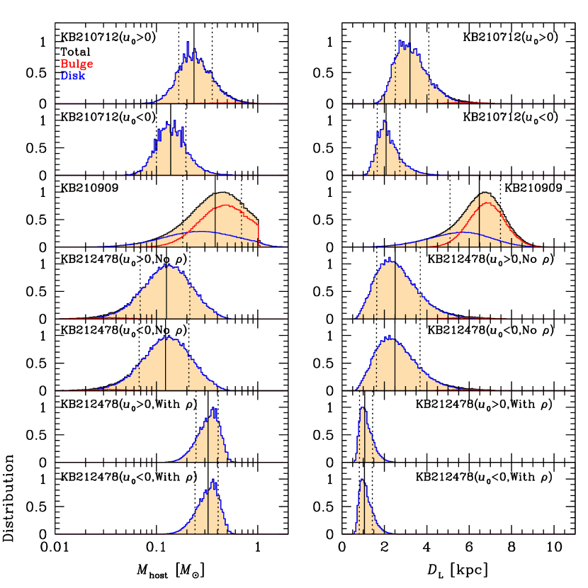
Figure 10: Host-mass and system-distance distributions from Bayesian analyses of various models (after imposing various constraints) for three of the events analyzed in this paper, KMT-2021-BLG-0712, KMT-2021-BLG-0909, and KMT-2021-BLG-2478. For the first and and last of these events, there are two models that are consistent with the light-curve data. For KMT-2021-BLG-2478, we consider two sets of constraints as described in Section 5.3. Bulge-lens and disk-lens distributions are shown in red and blue, respectively, while their total is shown in black.

The mass and distance distributions for the two solutions are shown in the top two rows of Figure 10.

The planet is intermediate in mass between Neptune and Saturn and orbits a mid-late M dwarf at about 3 kpc.

5.2 KMT-2021-BLG-0909

For this event, there is only one solution, for which there are two constraints: $t_{\rm E}=16.06\pm 0.73$ day (from Table 3) and $\theta_{\rm E}=0.362\pm 0.049$ mas (from Equation (16)). The mass and distance distributions are presented in the third row of Figure 10. These show that the system most likely lies in the Galactic bulge.

The planet is of Jovian mass and orbits a middle M dwarf at about 6.5 kpc.

5.3 KMT-2021-BLG-2478

For this event, there are three well-understood constraints (on $t_{\rm E}$, ${\mbox{\boldmath$\pi$}}_{\rm E}$, and $I_{L}$), and one constraint (on $\rho$) whose reliability must still be investigated. The first two constraints are given in Table 4, with the correlation coefficients for ${\mbox{\boldmath$\pi$}}_{\rm E}$ being $-0.02$ and $+0.04$ for $u_{0}>0$ and $u_{0}<0$, respectively. As discussed in Section 4.3, the constraint on lens light is $I_{L}>I_{B}=18.15$.

As discussed in Sections 3.4 and 4.3, the apparent constraints on $\rho$ from the light curve may be due to end-of-night systematics in the data, and they appear to be inconsistent with other constraints. We further investigate this by conducting Bayesian analyses with and without the $\rho$ constraint, which we implement as $\exp(-\chi^{2}(\rho)/2)$, where $\chi^{2}(\rho)$ is the envelope of $\chi^{2}$ with respect to $\rho$ (Figure 8) derived from the MCMC.

Table 8 shows the results of the Bayesian analysis with and without the constraint on $\rho$. It quantitatively confirms the concerns based on the qualitative reasoning given above. In particular, the “Galactic weights” are reduced by more than a factor of 100 by the imposition of the $\rho$ constraint, implying that this constraint is strongly inconsistent with the Bayesian priors from the Galactic model. When robust and well-understood measurements strongly conflict with priors, it can be strong evidence of new discoveries. However, in the present case, these conflicts arise from a handful of data points taken at high airmass. Hence, the “Adopted” parameters in Table 8 reflect the Bayesian analysis that suppresses the $\rho$ constraint.

The mass and distance distributions (bottom 4 rows of Figure 10) give another perspective on these same issues. In particular, the bottom two rows show that the $\rho$ constraint restricts the lens to being within $D_{L}<2\,{\rm kpc}$ of the Sun, which has very little phase space. Note, however, that with or without this constraint, bulge lenses are virtually excluded.

The planet is of Jovian mass and orbits a late M dwarf at about 2.5 kpc.

5.4 KMT-2021-BLG-1105

For this event there are two well-established constraints (on $t_{\rm E}$ and $\theta_{\rm E}$) as well as one potential constraint (on $I_{L}$) that remains to be investigated. The first, from Table 5, is $t_{\rm E}=35.0\pm 1.9\,$day (or $t_{\rm E}=35.4\pm 1.9\,$day). The second, as discussed in Section 4.4, is implemented via a $\chi^{2}(\rho)$ envelope function (Figure 9) together with an estimate for each simulated event with Einstein radius $\theta_{{\rm E},i}$, of $\rho_{i}=\theta_{*}/\theta_{{\rm E},i}$, with $\theta_{*}$ given by Table 7.

The potential constraint on $I_{L}$ comes from the limit $I_{L}\geq I_{B,\rm cal}$, where we calibrate the blend as $I_{B,\rm cal}=I_{B}-I_{\rm cl}+I_{\rm cl,0}+A_{I}=18.86$, with $I_{B}=19.00$ and $I_{\rm cl}-I_{\rm cl,0}=2.88$ coming from Table 7 and $A_{I}=2.75$ coming from the KMT webpage. The reason that this constraint is “potential” is that our investigation in Section 4.4 showed that the lens could be the origin of this blended light, in which case using it as a limit to exclude simulated events would bias the result toward lower masses. Thus, to check whether the “blend = lens” scenario is plausible within a Bayesian context, we first carry out the Bayesian analysis both with and without this constraint.

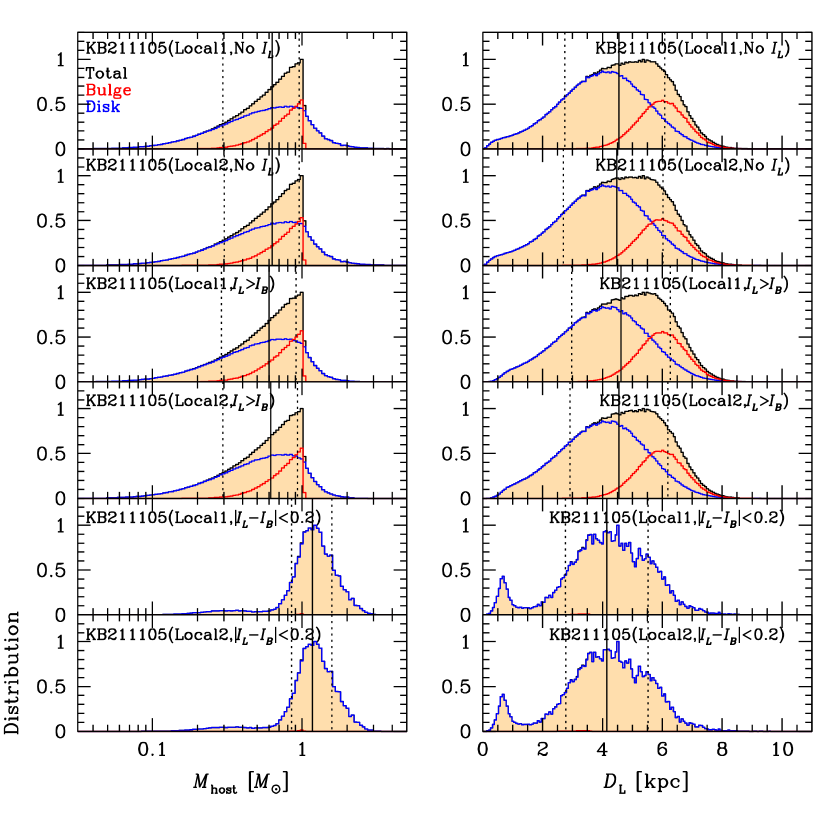
Figure 11: Host-mass and system-distance distributions from Bayesian analyses of two models (after imposing three different sets of constraints) for KMT-2021-BLG-1105. Color-coding is the same as Figure 10.

The results are given in Table 8 and illustrated in Figure 11. They show that the Bayesian estimates hardly change between the two cases. However, they also show that roughly 5% of the Galactic weight is eliminated by the flux constraint. This indicates that “blend = lens” hypothesis is consistent with the Bayesian priors at about the $2\,\sigma$ level (without yet taking into consideration the low probability of finding a random field star $\lesssim 0.1^{\prime\prime}$ of the event).

Therefore, we also conduct an additional Bayesian simulation under the constraint $|I_{L}-I_{B}|<0.2$. Note that the width of this interval is somewhat arbitrary: we just seek to distinguish simulated events that are roughly consistent with the “blend = lens” hypothesis from those that are not. The first point to note is that the host is a roughly solar mass star at $D_{L}\sim 4\,{\rm kpc}$. That is, it is substantially more massive than the unconstrained estimate, but roughly at the same distance. Second, at this distance, the lens system is located about 200 pc above the Galactic plane, and it therefore lies behind almost all the dust. Because $[(V-I)_{B}-(V-I)_{\rm cl}=-0.46$ (see Figure 7), this implies $(V-I)_{B,0}\simeq 0.60$, which is a very plausible value for a solar-mass (or slightly more massive) star.

Thus, we find that the “blend = lens” scenario is consistent with all the available constraints. On the other hand, the hypothesis that the blend is a companion to the lens is also plausible. In this case, the $\sim 0.1^{\prime\prime}$ astrometric offset would be explained by the companion being roughly 400 au from the host (rather than corruption of the astrometry by a faint field star).

We conclude that the blend is very likely to be either the host or a companion to the host. These scenarios could easily be distinguished by high resolution imaging by either AO on 8m class telescopes or the Hubble Space Telescope (HST). That is, a bright companion at $\sim 0.1^{\prime\prime}$ would easily be detected, which would verify the “blend = companion” scenario, while a contaminating random field star at several tenths of an arcsecond (verifying the “blend = lens” scenario) would be even more easily resolved. However, pending such a resolution, we advocate using the “no $I$ constraint” Bayesian analysis, which we treat as “Adopted” in Table 8.

If future high-resolution imaging (which could be done immediately) confirm the “blend = lens” hypothesis, then KMT-2021-BLG-1105Lb would be one of the rare microlensing planets that could be further studied using the radial velocity (RV) technique. If we adopt $M\simeq 1.1\,M_{\odot}$, which is consistent with both Table 8 and $(V-I)_{B,0}=0.60$, and we adopt $\pi_{\rm rel}\sim 0.13\,{\rm mas}$ (consistent with Table 8), then $\theta_{\rm E}\equiv\sqrt{\kappa M\pi_{\rm rel}}\simeq 1.1\,{\rm mas}$, and $a_{\perp}\sim 5.3\,{\rm au}$ (or 4.1 au). Considering that the semi-major axis is likely to be larger than the projected separation by a factor $\sim 1.5^{1/2}=1.22$, the orbital periods for Locals 1 and 2 are likely of order 16 and 11 years, respectively, with RV amplitudes of order $v\sin i\sim(25\,{\rm m\,s^{-1}})\sin i$ and $\sim(30\,{\rm m\,s^{-1}})\sin i$. Adopting $A_{I}/E(V-I)\sim 1.3$ from Figure 6 of Nataf et al. (2013), we obtain $V_{B,\rm cal}=I_{B,\rm cal}+(V-I)_{0}+A_{I}/1.3\simeq 21.6$. Hence, assuming that future high-resolution imaging confirms that the blend is the lens, it will be feasible to carry out RV measurements of the requisite precision on this $(I,V)\simeq(18.9,21.6)$ star on 30m class telescopes.

6 Discussion

This is the second in a series of papers that aims to publish all planets (and possible planets) that are detected by eye from 2021 KMTNet data and that are not published for other reasons. Together, we have presented a total of 8 such planets. In the course of these efforts, we identified a total of 7 other events that warranted detailed investigation but did not yield good planetary (or possibly planetary) solutions. Among the total of 15 events that were analyzed to prepare these two papers, none were possibly planetary but ultimately ambiguous. We have summarized that 8 other by-eye KMTNet planets have been published of which 7 will likely enter the AnomalyFinder statistical sample, as well as one possible planet. Thus, to date, there are a total of 16 planets from 2021 that are seemingly suitable for statistical analysis. These work-in-progress figures can be compared to 2018, which is the only year with a complete sample of KMTNet planets, as cataloged by Gould et al. (2022b) and Jung et al. (2022). In that case, of the 33 planets found by AnomalyFinder that were suitable for statistical studies, 22 were discovered by eye, while of the 8 possible planets, 3 were discovered by eye. That is, there were 22/3 discoveries for the full 2018 year compared to 16/1 discoveries for the partial 2021 year. Hence, this ongoing work is broadly consistent with the only previous comprehensive sample.

Table 1: Event Names, Cadences, Alerts, and Locations

Name	$\Gamma\,({\rm hr}^{-1})$	Alert Date	RAJ2000	DecJ2000	$l$	$b$
KMT-2021-BLG-0712	4.0	1 May 2021	17:57:08.56	$-$31:11:04.09	$-0.66$	$-3.29$
KMT-2021-BLG-0909	1.0	19 May 2021	17:42:28.85	$-$27:38:20.90	$+0.75$	$+1.27$
KMT-2021-BLG-2478	4.0	14 Sep 2021	17:57:14.21	$-29$:06:07.09	$+1.16$	$-2.27$
KMT-2021-BLG-1105	1.0	2 Jun 2021	17:42:55.74	$-25$:30:32.08	$+2.61$	$+2.30$

Note. — The coordinates given here are for the nearest catalog stars (i.e., baseline objects). In Section 4 we discuss the offsets from these locations of the actual events.

Table 2: Microlens Parameters for KMT-2021-BLG-0712

		Parallax models
Parameters	Standard	$u_{0}>0$	$u_{0}<0$
$\chi^{2}/\rm{dof}$	4263.666/4264	4224.244/4260	4222.276/4260
$t_{0}-2459340$	9.317 $\pm$ 0.115	9.954 $\pm$ 0.144	10.068 $\pm$ 0.129
$u_{0}$	0.147 $\pm$ 0.002	0.145 $\pm$ 0.002	-0.144 $\pm$ 0.002
$t_{\rm E}$ $(\rm{days})$	90.865 $\pm$ 0.951	88.503 $\pm$ 1.442	100.583 $\pm$ 2.039
$s$	1.196 $\pm$ 0.002	$1.196_{-0.012}^{+0.016}$	1.206 $\pm$ 0.020
$q$ $(10^{-4})$	4.751 $\pm$ 0.141	$5.121_{-0.654}^{+0.998}$	5.653 $\pm$ 1.157
log $q$ (mean)	-3.323 $\pm$ 0.014	-3.285 $\pm$ 0.062	-3.251 $\pm$ 0.079
$\alpha$ $(\rm{rad})$	0.467 $\pm$ 0.004	$0.452_{-0.034}^{+0.027}$	5.788 $\pm$ 0.039
$\rho$ $(10^{-4})$	3.903 $\pm$ 0.330	4.010 $\pm$ 0.449	4.221 $\pm$ 0.551
$\pi_{\rm{E},\it{N}}$	-	0.425 $\pm$ 0.104	0.701 $\pm$ 0.111
$\pi_{\rm{E},\it{E}}$	-	-0.047 $\pm$ 0.034	-0.204 $\pm$ 0.042
$ds/dt$ $(\rm{yr}^{-1})$	-	$0.008_{-0.199}^{+0.152}$	-0.149 $\pm$ 0.262
$d\alpha/dt$ $(\rm{yr}^{-1})$	-	$-0.688_{-0.321}^{+0.415}$	-0.902 $\pm$ 0.602
$I_{S}$ [KMTC01,pySIS]	21.618 $\pm$ 0.013	21.644 $\pm$ 0.017	21.653 $\pm$ 0.018
$I_{B}$ [KMTC01,pySIS]	18.676 $\pm$ 0.001	18.672 $\pm$ 0.002	18.673 $\pm$ 0.002
$t_{*}$ $(\rm{hours})$	0.851 $\pm$ 0.069	0.852 $\pm$ 0.092	1.019 $\pm$ 0.138

Table 3: Microlens Parameters for KMT-2021-BLG-0909

Parameters	2L1S
$\chi^{2}/\rm{dof}$	1636.961/1637
$t_{0}-2459350$	4.073 $\pm$ 0.017
$u_{0}$	0.060 $\pm$ 0.004
$t_{\rm E}$ $(\rm{days})$	16.046 $\pm$ 0.733
$s$	0.823 $\pm$ 0.008
$q$ $(10^{-3})$	3.174 $\pm$ 0.446
log $q$ (mean)	-2.497 $\pm$ 0.063
$\alpha$ $(\rm{rad})$	3.472 $\pm$ 0.012
$\rho$ $(10^{-3})$	3.326 $\pm$ 0.308
$I_{S}$ [KMTC,pySIS]	20.836 $\pm$ 0.060
$I_{B}$ [KMTC,pySIS]	17.503 $\pm$ 0.003
$t_{*}$ $(\rm{hours})$	1.284 $\pm$ 0.085

Table 4: Microlens Parameters for KMT-2021-BLG-2478

		Parallax + orbital motion models
Parameters	Standard	$u_{0}>0$	$u_{0}<0$
$\chi^{2}/\rm{dof}$	7720.303/7578	7573.830/7574	7574.077/7574
$t_{0}-2459480$	2.167 $\pm$ 0.018	2.243 $\pm$ 0.033	2.244 $\pm$ 0.033
$u_{0}$	0.081 $\pm$ 0.001	0.099 $\pm$ 0.002	-0.099 $\pm$ 0.002
$t_{\rm E}$ $(\rm{days})$	40.603 $\pm$ 0.402	33.689 $\pm$ 0.518	33.489 $\pm$ 0.511
$s$	1.058 $\pm$ 0.001	1.060 $\pm$ 0.002	1.060 $\pm$ 0.002
$q$ $(10^{-3})$	3.740 $\pm$ 0.121	6.087 $\pm$ 0.479	6.134 $\pm$ 0.480
log $q$ (mean)	-2.428 $\pm$ 0.015	-2.217 $\pm$ 0.034	-2.213 $\pm$ 0.034
$\alpha$ $(\rm{rad})$	0.274 $\pm$ 0.001	0.233 $\pm$ 0.014	6.051 $\pm$ 0.014
$\rho$ $(10^{-5})$	$2.403_{-1.736}^{+7.143}$	$2.452_{-1.763}^{+7.291}$	$1.915_{-1.392}^{+5.232}$
$\pi_{\rm{E},\it{N}}$	-	0.100 $\pm$ 0.209	0.113 $\pm$ 0.212
$\pi_{\rm{E},\it{E}}$	-	0.518 $\pm$ 0.064	0.522 $\pm$ 0.066
$ds/dt$ $(\rm{yr}^{-1})$	-	0.871 $\pm$ 0.165	0.872 $\pm$ 0.169
$d\alpha/dt$ $(\rm{yr}^{-1})$	-	1.285 $\pm$ 0.561	-0.918 $\pm$ 0.572
$I_{S}$ [KMTC(01),pySIS]	20.724 $\pm$ 0.013	20.497 $\pm$ 0.019	20.494 $\pm$ 0.019
$I_{B}$ [KMTC(01),pySIS]	17.971 $\pm$ 0.001	17.992 $\pm$ 0.002	17.992 $\pm$ 0.002
$t_{*}$ $(\rm{hours})$	$0.023_{-0.017}^{+0.070}$	$0.020_{-0.014}^{+0.059}$	$0.015_{-0.011}^{+0.042}$
$\beta$ $(\theta_{*}\equiv 0.4\mu{\rm as})$	-	$0.057_{-0.041}^{+0.145}$	$0.028_{-0.020}^{+0.083}$

Table 5: Microlens Parameters for KMT-2021-BLG-1105

Parameters	Local 1	Local 2	Local 3	Local 4
$\chi^{2}/\rm{dof}$	1784.854/1785	1788.955/1785	1795.837/1785	1806.507/1785
$t_{0}-2459370$	5.826 $\pm$ 0.036	5.856 $\pm$ 0.036	5.711 $\pm$ 0.036	5.780 $\pm$ 0.035
$u_{0}$	0.109 $\pm$ 0.007	0.107 $\pm$ 0.007	0.107 $\pm$ 0.007	0.101 $\pm$ 0.005
$t_{\rm E}$ $(\rm{days})$	34.965 $\pm$ 1.919	$35.374_{-1.739}^{+2.264}$	34.425 $\pm$ 1.985	$36.248_{-1.488}^{+1.887}$
$s$	1.214 $\pm$ 0.008	0.939 $\pm$ 0.008	1.265 $\pm$ 0.013	0.899 $\pm$ 0.010
$q$ $(10^{-3})$	1.984 $\pm$ 0.200	1.934 $\pm$ 0.191	4.939 $\pm$ 0.694	4.573 $\pm$ 0.614
log $q$ (mean)	-2.703 $\pm$ 0.044	-2.714 $\pm$ 0.043	-2.308 $\pm$ 0.062	-2.341 $\pm$ 0.058
$\alpha$ $(\rm{rad})$	2.140 $\pm$ 0.009	2.148 $\pm$ 0.010	2.136 $\pm$ 0.010	2.152 $\pm$ 0.009
$\rho$ $(10^{-3})$	$<1.3$	$<1.3$	$<1.3$	$<1.3$
$I_{S}$ [KMTC,pySIS]	21.233 $\pm$ 0.074	$21.258_{-0.070}^{+0.085}$	21.207 $\pm$ 0.080	21.294 $\pm$ 0.062
$I_{B}$ [KMTC,pySIS]	18.614 $\pm$ 0.006	18.612 $\pm$ 0.006	18.616 $\pm$ 0.006	18.609 $\pm$ 0.004
$t_{*}$ $(\rm{hours})$	$<1.1$	$<1.1$	$<1.1$	$<1.1$

Table 6: 1L2S for KMT-2021-BLG-1105

Parameters	1L2S	$\rho_{2}=0.001$	$\rho_{2}=0.0$
$\chi^{2}/\rm{dof}$	1790.359/1785	1800.137/1786	1803.805/1786
$t_{0,1}-2459370$	6.162 $\pm$ 0.041	6.151 $\pm$ 0.041	6.192 $\pm$ 0.043
$u_{0,1}$	0.105 $\pm$ 0.010	$0.077_{-0.005}^{+0.007}$	0.103 $\pm$ 0.010
$t_{\rm E}$ $(\rm{days})$	37.787 $\pm$ 3.115	49.293 $\pm$ 3.400	38.450 $\pm$ 3.202
$t_{0,2}-2459370$	3.389 $\pm$ 0.002	$3.388_{-0.004}^{+0.003}$	3.381 $\pm$ 0.004
$u_{0,2}$ $(10^{-3})$	0.000 $\pm$ 0.313	0.025 $\pm$ 0.322	0.654 $\pm$ 0.101
$\rho_{2}$ $(10^{-3})$	1.416 $\pm$ 0.139	1	-
$q_{F}$ $(10^{-2})$	1.021 $\pm$ 0.055	1.065 $\pm$ 0.072	1.186 $\pm$ 0.088
$I_{S}$ [KMTC,pySIS]	21.355 $\pm$ 0.113	$21.703_{-0.098}^{+0.080}$	21.381 $\pm$ 0.113
$I_{B}$ [KMTC,pySIS]	18.605 $\pm$ 0.007	$18.586_{-0.003}^{+0.005}$	18.603 $\pm$ 0.007
$I_{S,2}$ [KMTC,pySIS]	26.344 $\pm$ 0.103	$26.657_{-0.106}^{+0.065}$	26.211 $\pm$ 0.111
$t_{*,2}$ $(\rm{hours})$	1.284 $\pm$ 0.068	1.183 $\pm$ 0.082	-

Table 7: CMD Parameters for Four 2021 Planets

Parameter	KB210712	KB210909	KB212478	KB211105
$(V-I)_{\rm s}$	1.78$\pm$0.05	N.A.	2.05$\pm$0.05	2.50$\pm$0.08
$(V-I)_{\rm cl}$	2.15$\pm$0.03	N.A.	2.35$\pm$0.03	3.05$\pm$0.04
$(V-I)_{\rm cl,0}$	1.06	1.06	1.06	1.06
$(V-I)_{\rm s,0}$	0.69$\pm 0.06$	0.81$\pm$0.08	0.76$\pm$0.06	0.51$\pm$0.09
$I_{\rm s}$	21.75$\pm$0.02	20.80$\pm$0.06	20.37$\pm$0.03	21.49$\pm$0.07
$I_{\rm cl}$	15.83$\pm$0.05	17.95$\pm$0.05	15.97$\pm$0.05	17.25$\pm$0.05
$I_{\rm cl,0}$	14.48	14.41	14.39	14.37
$I_{\rm s,0}$	20.40$\pm$0.06	17.26$\pm$0.08	18.97$\pm$0.06	18.61$\pm$0.09
$\theta_{*}$ ($\mu{\rm as}$)	0.255$\pm 0.023$	1.205$\pm$0.163	0.533$\pm$0.043	0.482$\pm$0.053

Note. — Event names are abbreviations, e.g., KMT-2021-BLG-0712. $[(V-I),I]_{S}$ and $[(V-I),I]_{\rm cl}$ for KB210712 and KB212478 are based on calibrated OGLE-III photometry, while the other two events have instrumental KMT photometry.

Table 8: Physical properties

Event						Relative Weights
Models	Physical Properties					Gal.Mod.	$\chi^{2}$
KB210712	$M_{\rm host}$ $[M_{\sun}]$	$M_{\rm planet}$ $[M_{\earth}]$	$D_{\rm L}$ [kpc]	$a_{\bot}$ [au]
$u_{0}>0$	$0.23_{-0.07}^{+0.12}$	$39.90_{-11.90}^{+20.60}$	$3.20_{-0.68}^{+0.91}$	$2.29_{-0.42}^{+0.64}$		1.000	0.374
$u_{0}<0$	$0.14_{-0.04}^{+0.06}$	$25.76_{-7.11}^{+11.28}$	$2.08_{-0.42}^{+0.65}$	$1.57_{-0.26}^{+0.42}$		0.055	1.000
Adopted	$0.22_{-0.07}^{+0.12}$	$38.19_{-12.24}^{+20.52}$	$3.09_{-0.75}^{+0.94}$	$2.22_{-0.48}^{+0.66}$
KB210909	$M_{\rm host}$ $[M_{\sun}]$	$M_{\rm planet}$ $[M_{J}]$	$D_{\rm L}$ [kpc]	$a_{\bot}$ [au]
	$0.38_{-0.20}^{+0.30}$	$1.26_{-0.66}^{+1.01}$	$6.48_{-1.38}^{+1.00}$	1.75 $\pm$ 0.42
KB212478	$M_{\rm host}$ $[M_{\sun}]$	$M_{\rm planet}$ $[M_{J}]$	$D_{\rm L}$ [kpc]	$a_{\bot}$ [au]
No $\rho$ constraint
$u_{0}>0$	$0.12_{-0.06}^{+0.09}$	$0.80_{-0.35}^{+0.56}$	$2.51_{-0.87}^{+1.18}$	1.38 $\pm$ 0.26		1.000	1.000
$u_{0}<0$	$0.12_{-0.05}^{+0.09}$	$0.79_{-0.35}^{+0.56}$	$2.50_{-0.87}^{+1.18}$	1.37 $\pm$ 0.26		0.987	0.884
With $\rho$ constraint
$u_{0}>0$	0.33 $\pm$ 0.08	2.08 $\pm$ 0.52	$1.06_{-0.24}^{+0.37}$	1.64 $\pm$ 0.20		0.0008	1.000
$u_{0}<0$	0.32 $\pm$ 0.08	2.08 $\pm$ 0.52	$1.06_{-0.24}^{+0.37}$	1.64 $\pm$ 0.20		0.0008	0.884
Adopted	$0.12_{-0.06}^{+0.09}$	$0.80_{-0.35}^{+0.56}$	$2.50_{-0.87}^{+1.18}$	1.38 $\pm$ 0.26
KB211105	$M_{\rm host}$ $[M_{\sun}]$	$M_{\rm planet}$ $[M_{J}]$	$D_{\rm L}$ [kpc]	$a_{\bot}$ [au]
No $I_{L}$ constraint
Local 1	0.63 $\pm$ 0.33	1.30 $\pm$ 0.68	4.55 $\pm$ 1.67	$3.64_{-1.19}^{+0.93}$		1.000	1.000
Local 2	0.63 $\pm$ 0.33	1.28 $\pm$ 0.67	4.48 $\pm$ 1.66	$2.82_{-0.93}^{+0.72}$		0.975	0.129
$I_{L}>I_{B}$ constraint
Local 1	0.61 $\pm$ 0.31	1.27 $\pm$ 0.65	4.62 $\pm$ 1.65	$3.60_{-1.14}^{+0.89}$		0.946	1.000
Local 2	0.61 $\pm$ 0.32	1.24 $\pm$ 0.64	4.55 $\pm$ 1.64	$2.78_{-0.89}^{+0.69}$		0.920	0.129
$|I_{L}-I_{B}|<0.2$ const.
Local 1	$1.17_{-0.31}^{+0.42}$	$2.43_{-0.64}^{+0.88}$	4.14 $\pm$ 1.38	4.79 $\pm$ 0.87		0.023	1.000
Local 2	$1.17_{-0.31}^{+0.42}$	$2.37_{-0.63}^{+0.85}$	4.15 $\pm$ 1.38	3.70 $\pm$ 0.67		0.024	0.129
Adopted	0.63 $\pm$ 0.33	1.30 $\pm$ 0.68	4.54 $\pm$ 1.67	3.54 $\pm$ 1.06

Figure 6: Caustic topologies and source trajectories for each of the four solutions of KMT-2021-BLG-1105. Locals 1 and 2 constitute an “inner/outer” degenerate pair satisfying $s^{\dagger}_{+}\simeq s^{\dagger}\equiv\sqrt{s_{\rm inner}s_{\rm outer}}$ to high precision (Equation (10)), while Locals 3 and 4 constitute a second such pair that satisfy this equation equally well. The first pair are ridge-crossing, while the second pair are cusp crossing. The first pair are favored by $\Delta\chi^{2}>10$ and hence are adopted here.

References

- Alard & Lupton (1998) Alard, C. & Lupton, R.H.,1998, ApJ, 503, 325
- Albrow (2017) Albrow, M.D. Michaeldalbrow/Pydia: InitialRelease On Github., vv1.0.0, Zenodo
- Albrow et al. (2009) Albrow, M. D., Horne, K., Bramich, D. M., et al. 2009, MNRAS, 397, 2099
- An & Gould (2001) An, J.H., & Gould, A. 2001, ApJ, 563, L111
- An et al. (2002) An, J.H., Albrow, M.D., Beaulieu, J.-P. et al. 2002, ApJ, 572, 521
- Benedict et al. (2016) Benedict, G.F., Henry, T.J., Franz, O.G., et al. 2016, AJ, 152, 141
- Bensby et al. (2013) Bensby, T. Yee, J.C., Feltzing, S. et al. 2013, A&A, 549, A147
- Bessell & Brett (1988) Bessell, M.S., & Brett, J.M. 1988, PASP, 100, 1134
- Dong et al. (2009) Dong, S., Gould, A., Udalski, A., et al. 2009, ApJ, 695, 970
- Gaudi (1998) Gaudi, B.S. 1998, ApJ, 506, 533
- Gould (1992) Gould, A. 1992, ApJ, 392, 442
- Gould (2000) Gould, A. 2000, ApJ, 542, 785
- Gould (2004) Gould, A. 2004, ApJ, 606, 319
- Gould et al. (2021a) Gould, A., Zang, W., Mao, S., & Dong, S., 2021a, RAA, 21, 133
- Gould et al. (2022a) Gould, A., Jung, Y.K., Hwang, K.-H.,, et al. 2022a, JKAS, submitted, arXiv:2204.03269
- Gould et al. (2022b) Gould, A., Han, C., Zang, W., et al. 2022b, A&A, in press, arXiv:2204.04354
- Han & Gould (1995) Han, C. & Gould, A. 1995, ApJ, 447, 53
- Han (2006) Han, C. 2006, ApJ, 638, 1080
- Han et al. (2021a) Han, C., Udalski, A., Kim, D., et al. 2021a, A&A, 650A, 89
- Han et al. (2021b) Han, C., Gould, A., Hirao, Y., et al. 2021b, A&A, 655A, 24
- Han et al. (2022a) Han, C., Bond, I.A., Yee, J.C., et al. 2022a, A&A, 658A, 94
- Han et al. (2022b) Han, C., Gould, A., Bond, I.A., et al. 2022b, A&A, 662A, 70
- Han et al. (2022c) Han, C., Gould, A., Doeon, K., et al. 2022c, A&A, submitted, arXiV:2204.11378
- Han et al. (2022d) Han, C., Doeon, K., Yang, H., et al. 2022d, A&A, submitted, arXiV:2204.11383
- Han et al. (2022e) Han, C., Doeon, K., Gould, A., et al. 2022e, A&A, submitted,
- Herrera-Martin et al. (2020) Herrera-Martin, A., Albrow, A., Udalski, A., et al. 2020, AJ, 159, 134
- Holtzman et al. (1998) Holtzman, J.A., Watson, A.M., Baum, W.A., et al. 1998, AJ, 115, 1946
- Hwang et al. (2019) Hwang, K.-H., Udalski, A., Bond, I.A., et al. 2018, AJ, 155, 259
- Hwang et al. (2022) Hwang, K.-H., Zang, W., Gould, A., et al.., 2022, AJ, 163, 43
- Jung et al. (2022) Jung, Y. K., Zang, W., Han, C., et al. 2022, in prep
- Jung et al. (2021) Jung, Y. K., Han, C., Udalski, A.,. et al. 2021, AJ, 161, 293
- Kervella et al. (2004) Kervella, P., Thévenin, F., Di Folco, E., & Ségransan, D. 2004, A&A, 426, 297
- Kim et al. (2016) Kim, S.-L., Lee, C.-U., Park, B.-G., et al. 2016, JKAS, 49, 37
- Kim et al. (2018b) Kim, D.-J., Hwang, K.-H., Shvartzvald, et al. 2018b, arXiv:1806.07545
- Minniti et al. (2017) Minniti, D., Lucas, P., VVV Team, 2017, yCAT 2348, 0
- Nataf et al. (2013) Nataf, D.M., Gould, A., Fouqué, P. et al. 2013, ApJ, 769, 88
- Paczyński (1986) Paczyński, B. 1986, ApJ, 304, 1
- Park et al. (2004) Park, B.-G., DePoy, D.L.., Gaudi, B.S., et al. 2004, ApJ, 609, 166
- Parsons et al. (2018) Parsons, S.G., Gänsocle. B.T., Marsh, T.R., et al. 2018, MNRAS, 481, 1083
- Ryu et al. (2022) Ryu, Y.-H., Jung, Y.K., Yang, H., et al. 2022, AJ, submitted, arXiv:2202.03022
- Schechter et al. (1993) Schechter, P.L., Mateo, M., & Saha, A. 1993, PASP, 105, 1342
- Smith et al. (2003) Smith, M., Mao, S., & Paczyński, B., 2003, MNRAS, 339, 925
- Szymański et al. (2011) Szymański, M.K., Udalski, A., Soszyński, I., et al. 2011, Acta Astron., 61, 83
- Tomaney & Crotts (1996) Tomaney, A.B. & Crotts, A.P.S. 1996, au, 112, 2872
- Wang et al. (2022) Wang, H., Zang, W., Zhu, W, et al. 2022, MNRAS, 510, 1778
- Yang et al. (2022) Yang, H., Zang, W., Gould, A., et al. 2022, MNRAS, submitted, arXiv:2205.12584
- Yoo et al. (2004) Yoo, J., DePoy, D.L., Gal-Yam, A. et al. 2004, ApJ, 603, 139
- Zang et al. (2021b) Zang, W., Hwang, K.-H., Udalski, A., et al. 2021b, AJ, 162, 163
- Zang et al. (2022) Zang, W., Yang, H., Han, c., et al. 2022, arXiv:2204.02017
- Zhang & Gaudi (2022) Zhang, K. & Gaudi, B.S. 2022, arXiv:2205.05085