Riemannian Natural Gradient Methods

Abstract

This paper studies large-scale optimization problems on Riemannian manifolds whose objective function is a finite sum of negative log-probability losses. Such problems arise in various machine learning and signal processing applications. By introducing the notion of Fisher information matrix in the manifold setting, we propose a novel Riemannian natural gradient method, which can be viewed as a natural extension of the natural gradient method from the Euclidean setting to the manifold setting. We establish the almost-sure global convergence of our proposed method under standard assumptions. Moreover, we show that if the loss function satisfies certain convexity and smoothness conditions and the input-output map satisfies a Riemannian Jacobian stability condition, then our proposed method enjoys a local linear—or, under the Lipschitz continuity of the Riemannian Jacobian of the input-output map, even quadratic—rate of convergence. We then prove that the Riemannian Jacobian stability condition will be satisfied by a two-layer fully connected neural network with batch normalization with high probability, provided that the width of the network is sufficiently large. This demonstrates the practical relevance of our convergence rate result. Numerical experiments on applications arising from machine learning demonstrate the advantages of the proposed method over state-of-the-art ones.

90C06, 90C22, 90C26, 90C56

1 Introduction

Manifold constrained learning problems are ubiquitous in machine learning, signal processing, and deep learning. In this paper, we focus on manifold optimization problems of the form

(1.1) $$\min_{\Theta\in\mathcal{M}} \Psi(\Theta):=-\frac{1}{|\mathcal{S}|}\sum_{(x,y)\in\mathcal{S}}\log p(y|f(x,\Theta)),$$

where $\mathcal{M}\subseteq\mathbb{R}^{m\times n}$ is an embedded Riemannian manifold, $\Theta\in\mathcal{M}$ is the parameter to be estimated, $\mathcal{S}$ is a collection of $|\mathcal{S}|$ data pairs $(x,y)$ with $x\in\mathcal{X},y\in\mathcal{Y}$, $\mathcal{X}$ and $\mathcal{Y}$ are the input and output spaces, respectively, $f(\cdot,\Theta):\mathcal{X}\rightarrow\mathcal{Y}$ is a mapping from the input space to the output space, and $p(y|f(x,\Theta))$ is the conditional probability of taking $y$ conditioning on $f(x,\Theta)$. If the conditional distribution is assumed to be Gaussian, the objective function in (1.1) reduces to the square loss. When the conditional distribution $p(y|f(x,\Theta))$ obeys the multinomial distribution, the corresponding objective function is the cross-entropy loss. As an aside, it is worth noting the equivalence between the negative log probability loss and Kullback-Leibler (KL) divergence shown in [37].

Let us take the low-rank matrix completion (LRMC) problem [13, 31] as an example and explain how it can be fitted into the form (1.1). The goal of LRMC is to recover a low-rank matrix from an observed matrix $X$ of size $n\times N$. Denote by $\Omega$ the set of indices of known entries in $X$, the rank-$p$ LRMC problem amounts to solving

(1.2) $$\min_{U\in\mathrm{Gr}(n,p),A\in\mathbb{R}^{p\times N}}\frac{1}{2}\left\|\mathcal{P}_{\Omega}(UA-X)\right\|^{2},$$

where $\mathrm{Gr}(n,p)$ is the Grassmann manifold consists of all $p$-dimensional subspaces in $\mathbb{R}^{n}$. The operator $\mathcal{P}_{\Omega}(X)$ is defined in an element-wise manner with $\mathcal{P}_{\Omega}(X_{ij})=X_{ij}$ if $(i,j)\in\Omega$ and $0$ otherwise. Partitioning $X=\left[x_{1},\ldots,x_{N}\right]$ leads to the following equivalent formulation

$$\min_{U\in\mathrm{Gr}(n,p),a_{i}\in\mathbb{R}^{p}}\frac{1}{2N}\sum_{i=1}^{N}\left\|\mathcal{P}_{\Omega_{x_{i}}}\left(Ua_{i}-{x}_{i}\right)\right\|^{2},$$

where $x_{i}\in\mathbb{R}^{n}$ and the $j$-th element of $\mathcal{P}_{\Omega_{x_{i}}}(v)$ is $v_{j}$ if $(i,j)\in\Omega$ and $0$ otherwise. Given $U$, we can obtain ${a}_{i}$ by solving a least squares problem, i.e.,

$$a_{i}=a(U;x_{i}):=\operatorname*{arg\,min}_{a}\|\mathcal{P}_{\Omega_{x_{i}}}(Ua-x_{i})\|^{2}.$$

Then, the LRMC problem can be written as

(1.3) $$\min_{U\in\mathrm{Gr}(n,p)}\;\;\Psi(U):=\frac{1}{2N}\sum_{i=1}^{N}\|\mathcal{P}_{\Omega_{x_{i}}}\left(Ua(U;x_{i})-x_{i}\right)\|^{2}.$$

For the Gaussian distribution $p(y|z)=\frac{1}{\sqrt{(2\pi)^{n}}}\exp(-\frac{1}{2}(y-z)^{\top}(y-z))$, it holds that $-\log p(y|z)=\frac{1}{2}\|y-z\|^{2}+\frac{n\log(2\pi)}{2}$. Hence, problem (1.3) is a special case of problem (1.1), in which $\mathcal{S}=\{(x_{i},0)\}_{i=1}^{N}$, $\mathcal{X}=\mathbb{R}^{n}$, $\mathcal{Y}=\mathbb{R}^{n}$, $f(x,U)=\mathcal{P}_{\Omega_{x}}\left(Ua(U;x)-x\right)$, $\mathcal{M}=\mathrm{Gr}(n,p)$, and $p(y|z)=\frac{1}{\sqrt{(2\pi)^{n}}}\exp(-\frac{1}{2}(y-z)^{\top}(y-z))$. Other applications that can be fitted into the form (1.1) will be introduced in Section 4.

1.1 Motivation of this work

Since the calculation of the gradient of $\Psi$ in (1.1) can be expensive when the dataset $\mathcal{S}$ is large, various approximate or stochastic methods for solving (1.1) have been proposed. On the side of first-order methods, we have the stochastic gradient method [45], stochastic variance-reduced gradient method [30], and adaptive gradient methods [19, 34] for solving (1.1) in the Euclidean setting (i.e., $\mathcal{M}=\mathbb{R}^{m\times n}$). We refer the reader to the book [36] for variants of these algorithms and a comparison of their performance. For the general manifold setting, by utilizing manifold optimization techniques [1, 26, 12], Riemannian versions of the stochastic gradient method [11], stochastic variance-reduced gradient method [49, 64, 28], and adaptive gradient methods [10] have been developed.

On the side of second-order methods, existing algorithms for solving (1.1) in the Euclidean setting (i.e., $\mathcal{M}=\mathbb{R}^{m\times n}$) can be divided into two classes. The first is based on approximate Newton or quasi-Newton techniques; see, e.g., [46, 43, 15, 57, 58, 21, 44]. The second is the natural gradient-type methods, which are based on the Fisher information matrix (FIM) [4]. When the FIM can be approximated by a Kronecker-product form, the natural gradient direction can be computed using relative low computational cost. It is well known that second-order methods can accelerate convergence by utilizing curvature information. In particular, natural gradient-type methods can perform much better than the stochastic gradient method [38, 60, 7, 59, 9, 41] in the Euclidean setting. The connections between natural gradient methods and second-order methods have been established in [37]. Compared with the approximate Newton/quasi-Newton-type methods, methods based on FIM are shown to be more efficient when tackling large-scale learning problems. For the general manifold setting, Riemannian stochastic quasi-Newton-type and Newton-type methods [33, 32, 62] have been proposed by utilizing the second-order manifold geometry and variance reduction techniques. However, to the best of our knowledge, there is currently no Riemannian natural gradient-type method for solving (1.1). In view of the efficiency of Euclidean natural gradient-type methods, we are motivated to develop their Riemannian analogs for solving (1.1).

1.2 Our contributions

In this paper, we develop a new Riemannian natural gradient method for solving (1.1). Our main contributions are summarized as follows.

• We introduce the Riemannian FIM (RFIM) and Riemannian empirical FIM (REFIM) to approximate the Riemannian Hessian. These notions extend the corresponding ones for the Euclidean setting [4, 37] to the manifold setting. Then, we propose an adaptive regularized Riemannian natural gradient descent (RNGD) method. We show that for some representative applications, Kronecker-factorized approximations of RFIM and REFIM can be constructed, which reduce the computational cost of the Riemannian natural gradient direction. Our experiment results demonstrate that although RNGD is a second-order-type method, it has low per-iteration cost and enjoy favorable numerical performances.

• Under some mild conditions, we prove that RNGD globally converges to a stationary point of (1.1) almost surely. Moreover, if the loss function satisfies certain convexity and smoothness conditions and the input-output map $f$ satisfies a Riemannian Jacobian stability condition, then we can establish the local linear—or, under the Lipschitz continuity of the Riemannian Jacobian of $f$, even quadratic—rate of convergence of the method by utilizing the notion of second-order retraction. We then show that for a two-layer neural network with batch normalization, the Riemannian Jacobian stability condition will be satisfied with high probability when the width of the network is sufficiently large.

1.3 Notation

For an $m\times n$ matrix $\Theta$, we denote its Frobenius norm by $\|\Theta\|$ and its vectorization by $\theta=\mathrm{vec}(\Theta)\in\mathbb{R}^{mn}$. For a function $h:\mathbb{R}^{m\times n}\rightarrow\mathbb{R}$, we define its Euclidean gradient and Riemannian gradient on $\mathcal{M}$ by $\nabla h(\Theta)\in\mathbb{R}^{m\times n}$ and $\mbox{grad}\,h(\Theta)\in\mathbb{R}^{m\times n}$, respectively. For simplicity, we set $r=mn$. When no confusion can arise, we use $\nabla h(\theta)$ and $\mathrm{grad\!\;}h(\theta)$ to denote the vectorizations of $\nabla h(\Theta)$ and $\mathrm{grad\!\;}h(\Theta)$, respectively. We use $\nabla^{2}h(\theta)\in\mathbb{R}^{r\times r}$ and $\mathrm{Hess\!\;}h(\theta)\in\mathbb{R}^{r\times r}$ to denote the Euclidean Hessian and Riemannian Hessian of $h(\theta)$, respectively. We denote the tangent space to $\mathcal{M}$ at $\Theta$ by $T_{\Theta}\mathcal{M}$. We write $d\in T_{\theta}\mathcal{M}$ to mean ${\mathrm{mat}}(d)\in T_{\Theta}\mathcal{M}$, where $d\in\mathbb{R}^{r}$ and ${\mathrm{mat}}(d)$ converts $d$ into a $m$-by-$n$ matrix. For a retraction $R$ defined on $\mathcal{M}$, we write $R_{\theta}(d):=\mathrm{vec}(R_{\Theta}(D))\;\mathrm{for}\;D\in T_{\Theta}\mathcal{M}$, $\theta=\mathrm{vec}(\Theta)$, and $d=\mathrm{vec}(D)$. We shall use $\theta$ and $\Theta$ interchangeably when no confusion can arise. Basically, $\Theta$ is used when we want to utilize the manifold structure, while $\theta$ is used when we want to utilize the vector space structure of the ambient space.

1.4 Organization

We begin with the preliminaries on manifold optimization and natural gradient methods in Section 2. In Section 3, we introduce the RFIM and its empirical version REFIM and derive some of their properties. Then, we present our proposed RNGD method by utilizing the RFIM and REFIM. In Section 4, we discuss practical implementations of the RNGD method when problem (1.1) enjoys certain Kronecker-product structure. In Section 5, we study the convergence behavior of the RNGD method under various assumptions. Finally, we present numerical results in Section 6.

2 Preliminaries

2.1 Manifold optimization

Consider the optimization problem

(2.1) $$\min_{\Theta\in\mathcal{M}}\;\;h(\Theta),$$

where $\mathcal{M}\subseteq\mathbb{R}^{m\times n}$ is an embedded Riemannian manifold and $h:\mathbb{R}^{m\times n}\rightarrow\mathbb{R}$ is a smooth function. The design and analysis of numerical algorithms for tackling (2.1) have been extensively studied over the years; see, e.g., [1, 26, 12] and the references therein. One of the key constructs in the design of manifold optimization algorithms is the retraction operator. A smooth mapping $R:T\mathcal{M}:=\cup_{\Theta\in\mathcal{M}}T_{\Theta}\mathcal{M}\rightarrow\mathcal{M}$ is called a retraction operator if

• $R_{\Theta}(0)=\Theta$,

• $\mathrm{D}R_{\Theta}(0)[\xi]:=\frac{\mathrm{d}}{\mathrm{d}t}R_{\Theta}(t\xi)\mid_{t=0}=\xi$, for all $\xi\in T_{\Theta}\mathcal{M}$.

We call $R$ a second-order retraction [1, Proposition 5.5.5] if $\mathcal{P}_{T_{\Theta}\mathcal{M}}\left(\frac{\mathrm{d}^{2}}{\mathrm{d}t^{2}}R_{\Theta}(t\xi)|_{t=0}\right)\\ =0$ for all $\Theta\in\mathcal{M}$ and $\xi\in T_{\Theta}\mathcal{M}$. Some examples of second-order retraction can be found in [3, Theorem 22]. In the $k$-th iteration, retraction-based methods for solving (2.1) update $\Theta^{k+1}$ by

$$\Theta^{k+1}=R_{\Theta^{k}}(td^{k}),$$

where $d^{k}$ is a descent direction in the tangent space $T_{\Theta^{k}}\mathcal{M}$ and $t>0$ is the step size. The retraction operator $R$ constrains the iterates on $\mathcal{M}$. For a compact manifold, we have the following fact [14], which will be used in our later analysis.

Proposition 2.1.

Let $\mathcal{M}$ be a compact embedded submanifold of $\mathbb{R}^{m\times n}$. For all $\Theta\in\mathcal{M}$ and $\xi\in T_{\Theta}\mathcal{M}$, there exists a constant $\alpha>0$ such that the following inequality holds:

(2.2) $$\|R_{\Theta}(\xi)-\Theta\|\leq\alpha\|\Theta\|,\;\forall\Theta\in\mathcal{M},\;\forall\xi\in T_{\Theta}\mathcal{M}.$$

2.2 Natural gradient descent method

The natural gradient descent (NGD) method was originally proposed in [4] to solve (1.1) in the Euclidean setting (i.e., $\mathcal{M}=\mathbb{R}^{m\times n}$). Suppose that $y$ follows the conditional distribution $P_{y|f(x,\Theta)}$. Consider the population loss under $P_{y|x}(\Theta):=P_{y|f(x,\Theta)}$, i.e.,

(2.3) $$\Phi(\Theta):=-\mathbb{E}_{P_{x}}\left[\mathbb{E}_{P_{y|x}(\Theta)}\log p(y|f(x,\Theta))\right].$$

When $P_{y|x}(\Theta)$ and $P_{x}$ are replaced by their empirical counterparts defined using $\mathcal{S}$, the population loss $\Phi(\Theta)$ reduces to the empirical loss $\Psi(\Theta)$. Now, the FIM associated with $\Phi$ is defined as

$$F(\theta):=\mathbb{E}_{P_{x}}[\mathbb{E}_{P_{y|x}(\theta)}[\nabla\log p(y|f(x,\theta))\nabla\log p(y|f(x,\theta))^{\top}]]\in\mathbb{R}^{r\times r}.$$

Under certain regularity condition [20], we can interchange the order of expectation and derivative to obtain $F(\theta)=\nabla^{2}\Phi(\theta)$. In what follows, we assume that such a regularity condition holds. Since the distribution of $x$ is unknown, we set $P_{x}$ to be the empirical distribution defined by $\mathcal{S}$. In practice, we may only be able to get hold of an empirical counterpart of $P_{y|x}(\Theta)$. The empirical FIM (EFIM) associated with $\Psi$ is then defined by replacing $P_{y|x}(\Theta)$ with its empirical counterpart [51], i.e.,

$$\bar{F}(\theta):=\frac{1}{|\mathcal{S}|}\sum_{(x,y)\in\mathcal{S}}\nabla\log p(y|f(x,\theta))\nabla\log p(y|f(x,\theta))^{\top}.$$

With the FIM, the natural gradient direction is given by

$$\tilde{\nabla}\Phi(\theta):=(F(\theta))^{-1}\nabla\Phi(\theta)\in\mathbb{R}^{r}.$$

It is shown in [5, Theorem 1] and [42, Proposition 1] that $\tilde{\nabla}\Phi(\theta)$ is the steepest descent direction in the sense that

$$-\frac{\tilde{\nabla}\Phi(\theta)}{\|\nabla\Phi(\theta)\|_{(F(\theta))^{-1}}}=\lim_{\epsilon\rightarrow 0}\frac{1}{\epsilon}\operatorname*{arg\,min}_{d\in\mathbb{R}^{r}:\operatorname{KL}\left(P_{x,y}(\theta+d)\|P_{x,y}(\theta)\right)\leq\epsilon^{2}/2}{\Phi(\theta+d)},$$

where $\|\nabla\Phi(\theta)\|_{(F(\theta))^{-1}}:=\sqrt{\nabla\Phi(\theta)(F(\theta))^{-1}\nabla\Phi(\theta)}$.

In the $k$-th iteration, the iterative scheme of NGD for minimizing (2.3) is

$$\theta^{k+1}=\theta^{k}-t_{k}\tilde{\nabla}\Phi(\theta^{k}),$$

where $t_{k}>0$ is a proper step size. In the case where $F(\theta)$ is computationally expensive or inaccessible, we use the EFIM instead of the FIM. The connections between NGD and second-order methods are presented in [37].

3 Riemannian natural gradient method

3.1 Fisher information matrix on manifold

When the parameter to be estimated $\Theta$ lies on an embedded manifold $\mathcal{M}$, the Euclidean natural gradient direction needs not lie on the tangent space to $\mathcal{M}$ at $\Theta$ and thus cannot be used as a search direction in retraction-based methods. To overcome this difficulty, we first introduce the RFIM, which is defined as

(3.1) $$F^{R}(\theta):=\mathbb{E}_{P_{x}}\left[\mathbb{E}_{P_{y|x}(\theta)}\left[\mathrm{grad\!\;}\log p(y|f(x,\theta))\mathrm{grad\!\;}\log p(y|f(x,\theta))^{\top}\right]\right]\in\mathbb{R}^{r\times r},$$

where $\mathrm{grad\!\;}\log p(y|f(x,\theta))$ is the Riemannian gradient of $\log p(y|f(x,\theta))$ with respect to $\theta$. Then, we define the Riemannian natural gradient direction $d^{R}(\theta)$ as

(3.2) $$d^{R}(\theta):=(F^{R}(\theta))^{-1}\mathrm{grad\!\;}\Phi(\theta)\in\mathbb{R}^{r}.$$

The following theorem justifies our definition of RFIM. It extends the corresponding results on FIM given in [5, Theorem 1] and [42, Proposition 1].

Theorem 3.1.

Let $\mathcal{M}\subseteq\mathbb{R}^{m\times n}$ be an embedded manifold and $\Phi:\mathcal{M}\rightarrow\mathbb{R}$ be the function given in (2.3). For any second-order retraction $R$ on $\mathcal{M}$, the steepest descent direction in the tangent space to $\mathcal{M}$ at $\Theta$ is given by $-d^{R}(\theta)$ in (3.2), i.e.,

$$\frac{-d^{R}(\theta)}{\|\mathrm{grad\!\;}\Phi(\theta)\|_{(F^{R}(\theta))^{-1}}}=\lim_{\epsilon\rightarrow 0}\frac{1}{\epsilon}\operatorname*{arg\,min}_{d\in T_{\theta}\mathcal{M}:\mathbb{E}_{P_{x}}\left[\mathrm{KL}\left(P_{y|x}(R_{\theta}(d))\|P_{y|x}(\theta)\right)\right]\leq\epsilon^{2}/2}\Phi(R_{\theta}(d)),$$

where $\|\mathrm{grad\!\;}\Phi(\theta)\|_{(F^{R}(\theta))^{-1}}=\sqrt{\mathrm{grad\!\;}\Phi(\theta)^{\top}(F^{R}(\theta))^{-1}\mathrm{grad\!\;}\Phi(\theta)}$.

Proof 3.1.

For $\Theta\in\mathcal{M}$, from the definition

$$\mathrm{KL}(P_{y|x}(\theta)||P_{y|x}(R_{\theta}(td)))=\mathbb{E}_{P_{y|x}(\theta)}\log p(y|f(x,\theta))-\mathbb{E}_{P_{y|x}(\theta)}\log p(y|f(x,R_{\theta}(td))),$$

we have

$$\frac{\mathrm{d}}{\mathrm{d}t}\mathrm{KL}(P_{y|x}(\theta)||P_{y|x}(R_{\theta}(td)))\mid_{t=0} =-\frac{\mathrm{d}}{\mathrm{d}t}\mathbb{E}_{P_{y|x}(\theta)}\log p(y|f(x,R_{\theta}(td)))\mid_{t=0}$$

$$=-d^{\top}\nabla\mathbb{E}_{P_{y|x}(\theta)}\log p(y|f(x,\theta)).$$

By definition of the Riemannian gradient, we obtain

$$d^{\top}\mathrm{grad\!\;}\mathrm{KL}(P_{y|x}(\theta)||P_{y|x}(R_{\theta}(td)))\mid_{t=0}=-d^{\top}\nabla\mathbb{E}_{P_{y|x}(\theta)}\log p(y|f(x,\theta)),\quad\forall d\in T_{\theta}\mathcal{M},$$

where $\mathrm{grad\!\;}\mathrm{KL}(P_{y|x}(\theta)\parallel P_{y|x}(R_{\theta}(td)))\mid_{t=0}\in T_{\theta}\mathcal{M}$. Then, we have

$$\mathrm{grad\!\;}\mathrm{KL}(P_{y|x}(\theta)\parallel P_{y|x}(R_{\theta}(td)))\mid_{t=0}=-\mathrm{grad\!\;}\mathbb{E}_{P_{y|x}(\theta)}\log p(y|f(x,\theta)).$$

Accordingly, using the Leibniz integral rule and the property of second-order retractions [1, Proposition 5.5.5], we have the second-order derivative

$$\frac{\mathrm{d}^{2}}{\mathrm{d}t^{2}}\mathrm{KL}(P_{y|x}(\theta)||P_{y|x}(R_{\theta}(td)))\mid_{t=0}$$

$$= \mathbb{E}_{P_{y|x}(\theta)}[d^{\top}\mathrm{grad\!\;}\log p(y|f(x,\theta))\left(\mathrm{grad\!\;}\log p(y|f(x,\theta))\right)^{\top}d].$$

It follows that $\mathrm{grad\!\;}\mathbb{E}_{P_{y|x}(\theta)}\log p(y|f(x,\theta))=0$. By the definition of $F^{R}$, we conclude that

$$\mathbb{E}_{P_{x}}\mathrm{KL}(P_{y|x}(\theta)||P_{y|x}(R_{\theta}(d))=\frac{1}{2}d^{\top}F^{R}(\theta)d+O(d^{3}),\quad\forall d\in T_{\theta}\mathcal{M}.$$

From the fact [42, Proposition 1] that

$$\frac{-A^{-1}\nabla h(\theta)}{\|\nabla h(\theta)\|_{A^{-1}}}=\lim_{\epsilon\rightarrow 0}\frac{1}{\epsilon}\operatorname*{arg\,min}_{d:\|d\|_{A}\leq\epsilon}h(\theta+d),$$

where $A$ is a positive definite matrix and $\|d\|_{A^{-1}}=\sqrt{d^{\top}A^{-1}d}$, we have

(3.3) $$\frac{-B^{-1}\nabla(\Phi\circ R_{\theta})(0)}{\|\nabla(\Phi\circ R_{\theta})(0)\|_{B^{-1}}}=\lim_{\epsilon\rightarrow 0}\frac{1}{\epsilon}\operatorname*{arg\,min}_{d\;\in T_{\theta}\mathcal{M}:\|d\|_{A}\leq\epsilon}\Phi(R_{\theta}(d)),$$

where $B:T_{\theta}\mathcal{M}\rightarrow T_{\theta}\mathcal{M}$ is a positive definite linear operator. Note that for all $u\in T_{\theta}\mathcal{M}$, it holds that

$$\nabla(\Phi\circ R_{\theta})(0)[u]=\nabla\Phi(R_{\theta}(0))[\mathrm{D}R_{\theta}(0)[u]]=u^{\top}\mathrm{grad\!\;}\Phi(\theta).$$

This gives

$$\nabla(\Phi\circ R_{\theta})(0)=\mathrm{grad\!\;}\Phi(\theta).$$

Substituting the above into (3.3) and letting $B=F^{R}(\theta)$, we have

(3.4) $$\frac{-(F^{R}(\theta))^{-1}\mathrm{grad\!\;}\Phi(\theta)}{\|\mathrm{grad\!\;}\Phi(\theta)\|_{(F^{R}(\theta))^{-1}}}=\lim_{\epsilon\rightarrow 0}\frac{1}{\epsilon}\operatorname*{arg\,min}_{d\in T_{\theta}\mathcal{M}:\|d\|_{F^{R}(\theta)}\leq\epsilon}\Phi(R_{\theta}(d)).$$

Therefore, we conclude that

$$\frac{-(F^{R}(\theta))^{-1}\mathrm{grad\!\;}\Phi(\theta)}{\|\mathrm{grad\!\;}\Phi(\theta)\|_{(F^{R}(\theta))^{-1}}}=\lim_{\epsilon\rightarrow 0}\frac{1}{\epsilon}\underset{d\in T_{\theta}\mathcal{M}:\mathbb{E}_{P_{x}}\left[\operatorname{KL}\left(P_{y|x}(\theta)||P_{y|x}(R_{\theta}(d))\right)\right]\leq\epsilon^{2}/2}{\arg\min}\Phi(R_{\theta}(d))$$

for any second-order retraction $R$.

Note that the Riemannian Hessian [2, Equation 7] of $\Phi$ at $\theta$ along $u\in T_{\theta}\mathcal{M}$ is given by

$$\mathrm{Hess\!\;}\Phi(\theta)[u]=\mathcal{P}_{T_{\theta}\mathcal{M}}\left(\nabla^{2}\Phi(\theta)[u]\right)-\mathcal{P}_{T_{\theta}\mathcal{M}}\mathrm{D}_{u}(\mathrm{grad\!\;}\Phi(\theta)).$$

Hence, we have $\mathrm{Hess\!\;}\Phi(\theta)=F^{R}(\theta)$ due to the fact that $\mathrm{grad\!\;}\Phi(\theta)=0$. Similar to EFIM, we can define REFIM as

(3.5) $$\bar{F}^{R}(\theta):=\frac{1}{|\mathcal{S}|}\sum_{(x,y)\in\mathcal{S}}\mathrm{grad\!\;}\log p(y|f(x,\theta))\mathrm{grad\!\;}\log p(y|f(x,\theta))^{\top}.$$

3.2 Algorithmic framework

In the $k$-th iteration, once we obtain an estimate $F_{k}$ of the RFIM associated with $\Phi$ or the REFIM associated with $\Psi$ at $\theta^{k}$, the Riemannian natural gradient direction in the tangent space to $\mathcal{M}$ at $\theta^{k}$ is computed by solving the following optimization problem:

(3.6) $$\begin{aligned} d^{k}=\operatorname*{arg\,min}_{d\in T_{\theta^{k}}\mathcal{M}}\quad m_{k}(d):=\Psi_{k}+\left\langle g^{k},d\right\rangle+\frac{1}{2}\left\langle(F_{k}+\lambda_{k}I)d,d\right\rangle\end{aligned},$$

where $\Psi_{k}$ and $g^{k}$ are stochastic estimates of $\Psi(\theta^{k})$ and $\mathrm{grad\!\;}\Psi(\theta^{k})$, respectively and $\lambda_{k}>0$ is usually updated adaptively by a trust region-like strategy. Since $F_{k}+\lambda_{k}I:T_{\theta^{k}}\mathcal{M}\rightarrow T_{\theta^{k}}\mathcal{M}$ is positive definite and $g^{k}\in T_{\theta^{k}}\mathcal{M}$, the solution of (3.6) is $d^{k}=-(F_{k}+\lambda_{k}I)^{-1}g^{k}.$ If the inverse of $F_{k}+\lambda_{k}I$ is costly to compute, then the truncated conjugated gradient method can be utilized [40].

Once $d^{k}$ is obtained, we construct a trial point

(3.7) $$z^{k}=R_{\theta^{k}}(d^{k}).$$

To measure whether $z^{k}$ leads to a sufficient decrease in the objective value, we first calculate the ratio $\rho_{k}$ between the reduction of $\Psi$ and the reduction of $m_{k}$. Since the exact evaluation of $\Psi$ is costly, one popular way [16] is to construct estimates $\Psi_{k}^{0}$ and $\Psi_{k}^{z^{k}}$ of $\Psi(\theta^{k})$ and $\Psi(z^{k})$, respectively. Then, we compute the ratio as

(3.8) $$\rho_{k}=\frac{\Psi_{k}^{z^{k}}-\Psi_{k}^{0}}{m_{k}(d^{k})-\Psi_{k}^{0}}.$$

Here, we take $\Psi_{k}=\Psi_{k}^{0}$ in the calculation of $m_{k}(d^{k})$. Lastly, we perform the update

(3.9) $$\theta^{k+1}=\left\{\begin{array}[]{ll}z^{k},&\text{ if }\rho_{k}\geq\eta_{1}\text{~{}and~{}}\|g^{k}\|\geq\frac{\eta_{2}}{\sigma_{k}},\\ \theta^{k},&\text{ otherwise, }\end{array}\right.$$

where $\eta_{1}\in(0,1)$ and $\eta_{2}>0$ are constants and $\sigma_{k}>0$ is used to control the regularization parameter $\lambda_{k}$. Indeed, to ensure the descent property of the original function $\Psi$, some assumptions on the accuracy of the estimates of $\Psi(\theta^{k})$, $\Psi(z^{k})$ and the model $m_{k}$ are needed, and they will be introduced later in the convergence analysis. Due to the error in the estimates, the regularization parameter $\lambda_{k+1}$ should not only depend on the ratio $\rho_{k}$ but also on the norm of the estimated Riemannian gradient $g^{k}$. In particular, we set $\lambda_{k+1}:=\sigma_{k+1}\|g^{k+1}\|$ and update $\sigma_{k+1}$ as

(3.10) $$\sigma_{k+1}=\left\{\begin{array}[]{ll}\max\left\{\sigma_{\min},\frac{1}{\gamma}\sigma_{k}\right\},&\text{ if }\rho_{k}\geq\eta_{1}\text{~{}and~{}}\|g^{k}\|>\frac{\eta_{2}}{\sigma_{k}},\\ \gamma\sigma_{k},&\text{ otherwise},\\ \end{array}\right.$$

where $\eta_{1}\in(0,1)$, $\eta_{2}>0$ are as before and $\sigma_{\min}>0$, $\gamma>1$ are parameters. Our proposed RNGD method is summarized in Algorithm 1.

1 Choose an initial point $\theta^{0}$ and parameters $\sigma_{0}>0$, $\sigma_{\min}>0$, $\lambda_{0}=\sigma_{0}\|g^{0}\|$, $\eta_{1}\in(0,1)$, $\eta_{2}>0$, and $\gamma>1$. Set $k=0$.

2while stopping conditions not met do

3      

4      Compute the estimated Riemannian gradient $g^{k}$ and the estimated Riemannian Fisher information matrix $F_{k}$.

5       Compute the negative natural gradient direction $d^{k}$ by solving (3.6) and compute the trial point $z^{k}$ by (3.7).

6       Update $\theta^{k+1}$ based on (3.9).

7       Update $\lambda_{k+1}$ based on (3.10).

8       $k\leftarrow k+1$.

Algorithm 1 Riemannian natural gradient descent (RNGD) for solving (1.1).

4 Practical Riemannian natural gradient descent methods

From the definition of RFIM and REFIM in Section 3, the computational cost of solving subproblem (3.6) may be high because of the vectorization of $\Theta$. Fortunately, analogous to [38], the Riemannian natural gradient direction can be computed with a relatively low cost if the gradient of a single sample is of low rank, i.e., for a pair of observations $(x,y)\in\mathcal{S}$ and $\psi(\Theta;x,y):=-\log p(y|f(x,\Theta))$, $\nabla\psi$ takes the form

(4.1) $$\nabla\psi(\Theta;x,y)=G(x,y)A(x,y)^{\top},$$

where $G(x,y)\in\mathbb{R}^{m\times q}$ and $A(x,y)\in\mathbb{R}^{n\times q}$ with $q\ll\min(m,n)$. Let us now elaborate on this observation.

Recall that the Riemannian gradient of $\psi$ is given by

$$\mathrm{grad\!\;}\psi(\Theta;x,y)=\mathcal{P}_{T_{\Theta}\mathcal{M}}(\nabla\psi(\Theta;x,y)).$$

When $\nabla\psi$ has the form (4.1), the linearity of the projection operator implies that

(4.2) $$F^{R}(\theta) =\mathbb{E}_{P_{x,y}(\theta)}\left[\mathrm{grad\!\;}\psi(\theta;x,y)\mathrm{grad\!\;}\psi(\theta;x,y)^{\top}\right]$$

$$\approx\mathcal{P}\left(\mathbb{E}_{P_{x,y}(\theta)}\left[A(x,y)A(x,y)^{\top}\right]\otimes\mathbb{E}_{P_{x,y}(\theta)}\left[G(x,y)G(x,y)^{\top}\right]\right)\mathcal{P},$$

where $P_{x,y}(\theta)$ is the joint distribution of $(x,y)$ given $\theta$, $\mathcal{P}\in\mathbb{R}^{r\times r}$ is the matrix representation of $\mathcal{P}_{T_{\Theta}\mathcal{M}}$ (note that $\mathcal{P}^{\top}=\mathcal{P}$ due to the symmetry of orthogonal projection operators), and the approximation is due to the assumption that $A(x,y)$ and $G(x,y)$ are approximately independent; see also [23, Theorem 1] for a use of such an assumption to derive a simplified form of the FIM. By replacing $P_{x,y}(\theta)$ with its empirical distribution observed from $\mathcal{S}$, an approximate REFIM is given by

(4.3) $$\bar{F}^{R}(\theta)\approx\mathcal{P}\left(\left[\frac{1}{|\mathcal{S}|}\sum_{(x,y)\in\mathcal{S}}A(x,y)A(x,y)^{\top}\right]\otimes\left[\frac{1}{|\mathcal{S}|}\sum_{(x,y)\in\mathcal{S}}G(x,y)G(x,y)^{\top}\right]\right)\mathcal{P}.$$

When a direct inverse of $\bar{F}^{R}(\theta)$ is expensive to compute, the truncated conjugated gradient method can be used. In preparation for the applications, we now show how to construct computationally efficient approximations of the RFIM and REFIM on the Grassmann manifold.

4.1 RFIM and REFIM on Grassmann manifold

If the matrix representation $\mathcal{P}$ of the projection operator $\mathcal{P}_{T_{\Theta}\mathcal{M}}$ has dimensions $m$-by-$m$ or $n$-by-$n$, i.e.,

$$\mathrm{grad\!\;}\psi(\Theta;x,y)=B_{1}G(x,y)A(x,y)^{\top}\;\;\mathrm{or}\;\;\mathrm{grad\!\;}\psi(\Theta;x,y)=G(x,y)A(x,y)^{\top}B_{2}$$

with $B_{1}\in\mathbb{R}^{m\times m}$ and $B_{2}\in\mathbb{R}^{n\times n}$, then we can approximate the RFIM in (4.2) by

$$F^{R}(\theta)\approx\mathbb{E}_{P_{x,y}(\theta)}\left[A(x,y)A(x,y)^{\top}\right]\otimes\mathbb{E}_{P_{x,y}(\theta)}\left[B_{1}G(x,y)G(x,y)^{\top}B_{1}\right]$$

or

$$F^{R}(\theta)\approx\mathbb{E}_{P_{x,y}(\theta)}\left[B_{2}A(x,y)A(x,y)^{\top}B_{2}\right]\otimes\mathbb{E}_{P_{x,y}(\theta)}\left[G(x,y)G(x,y)^{\top}\right].$$

Moreover, if we replace $P_{x,y}(\theta)$ by its empirical distribution observed from $\mathcal{S}$, then we can approximate the REFIM in (4.3) by

$$\bar{F}^{R}(\theta)\approx\left(\frac{1}{|\mathcal{S}|}\sum_{(x,y)\in\mathcal{S}}A(x,y)A(x,y)^{\top}\right)\otimes\left(\frac{1}{|\mathcal{S}|}\sum_{(x,y)\in\mathcal{S}}B_{1}G(x,y)G(x,y)^{\top}B_{1}\right)$$

or

$$\bar{F}^{R}(\theta)\approx\left(\frac{1}{|\mathcal{S}|}\sum_{(x,y)\in\mathcal{S}}B_{2}A(x,y)A(x,y)^{\top}B_{2}\right)\otimes\left(\frac{1}{|\mathcal{S}|}\sum_{(x,y)\in\mathcal{S}}G(x,y)G(x,y)^{\top}\right).$$

Note that the Kronecker product form allows the inverse of $\bar{F}^{R}(\theta)$ to be calculated efficiently by inverting two smaller matrices [38]. A typical manifold that yields the above Kronecker product representations is the Grassmann manifold $\mathrm{Gr}(m,n)$, which consists of all $n\;(\mathrm{resp.},\,m)$ dimensional subspaces in $\mathbb{R}^{m}\;(\mathrm{resp.},\,\mathbb{R}^{n})$ if $m\geq n$ (resp., $m<n$). The matrix representation of the projection operator is $B_{1}=I_{m}-\Theta\Theta^{\top}$ ($m\geq n$) or $B_{2}=I_{n}-\Theta^{\top}\Theta$ ($m<n$). In what follows, we derive the RFIMs associated with three concrete applications involving the Grassmann manifold and explain how they can be computed efficiently.

4.2 Applications

4.2.1 Low-rank matrix completion

For simplicity, we derive the RFIM associated with problem (1.3) for the fully observed case, i.e., $\Omega=\{1,\ldots,n\}\times\{1,\ldots,N\}$. One can derive the RFIM for the partly observed case in a similar fashion. By definition, we have $f(x,U)=Ua(U;x)-x$ and $\psi(U;x,y)=-\log p(y|f(x,U))=\frac{1}{2}\|f(x,U)-y\|^{2}+\frac{n\log(2\pi)}{2}$. It follows from [13] that the Jacobian of $a$ along a tangent vector $H\in T_{U}\mathrm{Gr}(n,p)$ is given by $J_{a}(U;x)[H]=H^{\top}x$ and its adjoint $J^{\top}_{a}(U;x)$ satisfies $J^{\top}_{a}(U;x)[v]=x^{\top}v$ for $v\in\mathbb{R}^{p}$. The Riemannian gradient of $\psi(\cdot;x,y)$ is

$$\mathrm{grad\!\;}\psi(U;x,y)= (I-UU^{\top})((Ua(U;x)-x-y)a(U;x)^{\top})$$

$$+(I-UU^{\top})x(Ua(U;x)-x-y)^{\top}U.$$

By assuming that the residual $Ua(U;x)-x$ is close to zero, we have$(I-UU^{\top})x\approx(I-UU^{\top})Ua(U;x)=0$. This leads to the following approximate Riemannian gradient of $\psi(\cdot;x,y)$:

(4.4) $$\mathrm{grad\!\;}\psi(U;x,y)\approx(I-UU^{\top})((Ua(U;x)-x-y)a(U;x)^{\top}).$$

Plugging the above approximation into (4.2) leads to

$$F^{R}(u)= \mathbb{E}_{P_{x}}\left[\mathbb{E}_{P_{y|x}(u)}\left[\mathrm{grad\!\;}\psi(u;x,y)\mathrm{grad\!\;}\psi(u;x,y)^{\top}\right]\right]$$

$$\approx \mathbb{E}_{P_{x}}\left[\mathbb{E}_{P_{y|x}(U)}\left[[a(U;x)a(U;x)^{\top}]\otimes\left[(I-UU^{\top})(Ua(U;x)-x-y)\right.\right.\right.$$

$$\left.\left.\left.(Ua(U;x)-x-y)^{\top}(I-UU^{\top})\right]\right]\right]$$

$$\approx \left[\frac{1}{N}\sum_{i=1}^{N}a(U;x_{i})a(U;x_{i})^{\top}\right]\otimes(I-UU^{\top}),$$

where $u=\mathrm{vec}(U)$ is the vectorization of $U$, the second line is due to (4.4), $\mathrm{vec}(uv^{\top})=v\otimes u$, $(A\otimes B)^{\top}=A^{\top}\otimes B^{\top}$, and $(A\otimes B)(A^{\top}\otimes B^{\top})=(AA^{\top})\otimes(BB^{\top})$, and the last line follows from $\mathbb{E}_{P_{y|x}(U)}\left[(Ua(U;x)-x-y)(Ua(U;x)-x-y)^{\top}\right]=I$ and by substituting $P_{x}$ with its empirical distribution. For $H\in T_{U}\mathrm{Gr}(n,p)$, we have

(4.5) $$\mathrm{mat}(F^{R}(u)[\mathrm{vec}(H)]) \approx\left[\frac{1}{N}\sum_{i=1}^{N}a(U;x_{i})a(U;x_{i})^{\top}\right]\otimes(I-UU^{\top})\mathrm{vec}(H)$$

$$=H\left[\frac{1}{N}\sum_{i=1}^{N}a(U;x_{i})a(U;x_{i})^{\top}\right],$$

where $\mathrm{mat}(b)$ converts the vector $b\in\mathbb{R}^{np}$ into an $n$-by-$p$ matrix and the equality follows from $(I-UU^{\top})H=H$. For the partly observed case, the matrix $F^{R}(u)$ defined in the above equation can serve as a good approximation of the exact RFIM. Note that $\frac{1}{N}\sum_{i=1}^{N}a(U;x_{i})a(U;x_{i})^{\top}\in\mathbb{R}^{p\times p}$ is of low dimension since the rank $p$ is usually small. Thus, the Riemannian natural gradient direction can be calculated with a relatively low cost.

4.2.2 Low-dimension subspace learning

In multi-task learning [6, 39], different tasks are assumed to share the same latent low-dimensional feature representation. Specifically, suppose that the $i$-th task has the training set $X_{i}\in\mathbb{R}^{d_{i}\times n}$ and the corresponding label set $y_{i}\in\mathbb{R}^{d_{i}}$ for $i=1,\ldots,N$. The multi-task feature learning problem can then be formulated as

(4.6) $$\min_{U\in\text{Gr}(n,p)}\Psi(U)=\frac{1}{2N}\sum_{i=1}^{N}\|X_{i}Uw(U;X_{i},y_{i})-y_{i}\|^{2},$$

where $w(U;X_{i},y_{i})=\arg\min_{w}\frac{1}{2}\|X_{i}Uw-y_{i}\|^{2}+\lambda\|w\|^{2}$ and $\lambda>0$ is a regularization parameter. Suppose that $d_{1}=\cdots=d_{N}=d$. Then, problem (4.6) has the form (1.1), where $\mathcal{S}=\{((X_{i},y_{i}),0)\}_{i=1}^{N}$, $\mathcal{X}=\mathbb{R}^{d\times(n+1)},\;\mathcal{Y}=\mathbb{R}^{d}$, $f(X,y,U)=XUw(U;X,y)-y$, and $p(z|f(X,y,U))=\frac{1}{\sqrt{(2\pi)^{d}}}\exp(-\frac{1}{2}(z-f(X,y,U))^{\top}(z-f(X,y,U)))$. By ignoring the constant $\frac{d\log(2\pi)}{2}$ and slightly abusing the notation, we define $\psi(U;X,y,z)=\frac{1}{2}\|XUw(U;X,y)-y-z\|^{2}$. Using the optimality of $w(U;X,y)$, we have $U^{\top}X^{\top}(XU\\ w(U;X,y)-y)+\lambda w(U;X,y)=0$. Then, we can compute the Euclidean gradient of $\psi(\cdot;X,y,z)$ as

$$\nabla\psi(U;X,y,z)$$

$$= X^{\top}(XUw(U;X,y)-y-z)w(U;X,y)^{\top}+J_{w}^{\top}(U)\left[U^{\top}X^{\top}(XUw(U;X,y)-y-z)\right]$$

$$\approx X^{\top}(XUw(U;X,y)-y)w(U;X,y)^{\top},$$

where $J_{w}(U)$ is the Jacobian of $w(U;X,y)$, $J_{w}^{\top}(U)$ denotes the adjoint of $J_{w}(U)$, and the approximation holds for small $\lambda$ and $\|z\|$. Note that $z$ will lie in a small neighborhood of zero with high probability if $f(X,y,U)$ is close to 0. Besides, $z$ is always zero in the dataset $\mathcal{S}$. With the above, an approximate Riemannian gradient of $\psi(\cdot;X,y,z)$ is given by

(4.7) $$\mathrm{grad\!\;}\psi(U;X,y,z)\approx(I-UU^{\top})X^{\top}(XUw(U;X,y)-y-z)w(U;X,y)^{\top}.$$

Consequently, we have

(4.8) $$F^{R}(u) =\mathbb{E}_{P_{(X,y)}}\left[\mathbb{E}_{P_{z|(X,y)}(u)}[\mathrm{grad\!\;}\psi(u;X,y,z)\mathrm{grad\!\;}\psi(u;X,y,z)^{\top}]\right]$$

$$\approx \frac{1}{N}\sum_{i=1}^{N}(w_{i}\otimes((I-UU^{\top})X_{i}^{\top}))(w_{i}\otimes((I-UU^{\top})X_{i}^{\top}))^{\top}$$

$$= \frac{1}{N}\sum_{i=1}^{N}\left[(w_{i}w_{i}^{\top})\otimes((I-UU^{\top})X_{i}^{\top}X_{i}(I-UU^{\top}))\right]$$

$$\approx \frac{1}{N}\left[\sum_{i=1}^{N}w_{i}w_{i}^{\top}\right]\otimes\left[\frac{1}{N}\sum_{i=1}^{N}(I-UU^{\top})X_{i}^{\top}X_{i}(I-UU^{\top})\right],$$

where $u=\mathrm{vec}(U)$ is the vectorization of $U$, $w_{i}:=w(U;X_{i},y_{i})$, the second line follows from (4.7), $\mathbb{E}_{P_{z|(X,y)}(u)}[(XUw(U;X,y)-y-z)(XUw(U;X,y)-y-z)^{\top}]=I$, and the empirical approximation of $P_{(X,y)}$, and the last line holds under the same condition as in (4.2). Though the construction of $F^{R}(u)$ is for the case $d_{1}=\cdots=d_{N}$, it can be easily extended to the case where the $d_{i}$’s are not equal.

4.2.3 Fully connected network with batch normalization

Consider an $L$-layer neural network with input $a_{0}=x$. In the $l$-th layer, we have

(4.9) $$s_{l}=W_{l}a_{l-1}+b_{l},\;t_{l,i}=\frac{s_{l,i}-\mathbb{E}(s_{l,i})}{\operatorname{Var}(s_{l,i})}\times\gamma_{l,i}+\beta_{l,i},\;i=1,\ldots,n_{l},\;a_{l}=\varphi_{l}\left(t_{l}\right),$$

where $\varphi_{l}$ is an element-wise activation function, $W_{l}\in\mathbb{R}^{n_{l}\times n_{l-1}}$ is the weight, $b_{l}\in\mathbb{R}^{n_{l}}$ is the bias, $s_{l,i}$ is the $i$-th component of $s_{l}\in\mathbb{R}^{n_{l}}$, $\gamma_{l,i},\beta_{l,i}\in\mathbb{R}$ are two learnable parameters, $\mathrm{Var}(s_{l,i})$ is the variance of $s_{l,i}$, and $f(x,\Theta)=a_{L}\in\mathbb{R}^{m}$ is the output of the network with $\Theta$ being the collection of parameters $\{W_{l},b_{l},\gamma_{l},\beta_{l}\}$. By default, the elements of $\gamma_{l,i}$ are set to 1 and the elements of $\beta_{l,i}$ are set to 0. In [27], $t_{l,i}$ is called the batch normalization of $s_{l,i}$.

Given a dataset $\mathcal{S}$, our goal is to minimize the discrepancy between the network output $f(x,\Theta)$ and the observed output $y$, namely,

(4.10) $$\min_{\Theta}\;\;\Psi(\Theta)=-\frac{1}{|\mathcal{S}|}\sum_{(x,y)\in\mathcal{S}}\log p(y|f(x,\Theta)).$$

By [17], each row of $W_{l}$ lies on the Grassmann manifold $\mathrm{Gr}(1,n_{l-1})$. It follows that $W_{l}$ lies on the product of Grassmann manifolds, i.e., $W_{l}\in\mathrm{Gr}(1,n_{l-1})\times\cdots\times\mathrm{Gr}(1,n_{l-1})\in\mathbb{R}^{n_{l}\times n_{l-1}}$. The remaining parameters lie in the Euclidean space. Rather than batch normalization, layer normalization [8] and weight normalization [47] have also been widely investigated in the study of deep neural networks, where $\mathrm{vec}(W_{l})\in\mathrm{Gr}(n_{l}\times n_{l-1},1)$ and $W_{l}\in\mathrm{Sp}(n_{l-1}-1)\times\cdots\times\mathrm{Sp}(n_{l-1}-1)\in\mathbb{R}^{n_{l}\times n_{l-1}}$ with $\mathrm{Sp}(n_{l-1}-1):=\{u\in\mathbb{R}^{n_{l-1}}:\|u\|=1\}$, respectively.

By back-propagation, the Euclidean gradient of $\Psi$ with respect to $W_{l}$ is given by

$$g_{l}\leftarrow\mathrm{D}a_{l}\odot\varphi_{l}^{\prime}\left(t_{l}\right)\odot\mathrm{D}t_{l},\quad\nabla\Psi(W_{l})\leftarrow g_{l}a_{l-1}^{\top},\quad\mathrm{D}a_{l-1}\leftarrow W_{l}^{\top}g_{l}.$$

In particular, we see that $\nabla\Psi(W_{l})$ has the Kronecker product form (4.1). Moreover, note that $\Psi(w_{l,i})=\Psi(cw_{l,i}),\;\forall c\neq 0$. Now, we compute

$$\nabla\Psi(w_{l,i})w_{l,i}^{\top}=\lim_{t\rightarrow 0}\frac{\Psi(w_{l,i}+tw_{l,i})-\Psi(w_{l,i})}{t}=0.$$

By definition of the projection operator defined on the product of Grassmann manifolds, the Riemannian gradient $\mbox{grad}\,\Psi(W_{l})$ is actually the same as the Euclidean gradient $\nabla\Psi(W_{l})$. Specifically, for the $i$-th row of $\mathrm{grad\!\;}\Psi(W_{l})$, we have

$$\left[\mathrm{grad\!\;}\Psi(W_{l})\right]_{i}=\mathrm{grad\!\;}\Psi(w_{l,i})=\nabla\Psi(w_{l,i})-\nabla\Psi(w_{l,i})w_{l,i}^{\top}w_{l,i}=\nabla\Psi(w_{l,i}).$$

Therefore, the RFIM coincides with the FIM. The inverse of $F^{R}(\theta)$ can be computed easily when the FIM has a Kronecker product form.

5 Convergence Analysis

In this section, we study the convergence behavior of the RNGD method (Algorithm 1).

5.1 Global convergence to a stationary point

To begin, let us extend some of the definitions used in the study of Euclidean stochastic trust-region methods (see, e.g., [16]) to the manifold setting.

Definition 5.1.

Let $\kappa_{\rm ef},\kappa_{\rm eg}>0$ be given constants. A function $m_{k}$ is called a $(\kappa_{\rm ef},\kappa_{\rm eg})$-fully linear model of $\Psi$ on $B_{\theta^{k}}(0,1/\sigma_{k})$ if for any $y\in B_{\theta^{k}}(0,1/\sigma_{k})$,

(5.1) $$\|\nabla(\Psi\circ R_{\theta^{k}})(y)-\nabla m_{k}(y)\|\leq\frac{\kappa_{\rm eg}}{\sigma_{k}}\quad\textrm{and}\quad|\Psi\circ R_{\theta^{k}}(y)-m_{k}(y)|\leq\frac{\kappa_{\rm ef}}{\sigma_{k}^{2}},$$

where $B_{\theta}(0,\rho):=\left\{d\in T_{\theta}\mathcal{M}:\|d\|\leq\rho\right\}$.

Definition 5.2.

Let $\epsilon_{F},\sigma_{k}>0$ be given constants. The quantities $\Psi_{k}^{0}$ and $\Psi_{k}^{z^{k}}$ are called $\epsilon_{F}$-accurate estimates of $\Psi\left(\theta^{k}\right)$ and $\Psi_{k}\left(z^{k}\right)$, respectively if

(5.2) $$\left|\Psi_{k}^{0}-\Psi\left(\theta^{k}\right)\right|\leq\frac{\epsilon_{F}}{\sigma_{k}^{2}}\quad\text{ and }\quad\left|\Psi_{k}^{z^{k}}-\Psi_{k}\left(z^{k}\right)\right|\leq\frac{\epsilon_{F}}{\sigma_{k}^{2}},$$

where $z^{k}$ is defined in (3.7).

Analogous to [16, 55], the inequalities (5.1) and (5.2) can be guaranteed when $\mathcal{M}$ is compact, the number of samples is large enough, and $\nabla(\Psi\circ R)$ is Lipschitz continuous.

Next, we introduce the assumptions needed for our convergence analysis. Their Euclidean counterparts can be found in, e.g., [16, Assumptions 4.1 and 4.3].

Assumption 5.3.

Let $\theta^{0}\in\mathbb{R}^{r},\sigma_{\min}>0$ be given. Let $\mathcal{L}(\theta^{0})$ denote the set of iterates generated by Algorithm 1. Then, the function $\Psi$ is bounded from below on $\mathcal{L}(\theta^{0})$. Moreover, the function $\Psi\circ R$ and its gradient $\nabla(\Psi\circ R)$ are $L$-Lipschitz continuous on the set

$$\mathcal{L}_{\rm enl}(\theta^{0})=\bigcup_{\theta\in\mathcal{L}(\theta^{0})}B_{\theta}\left(0,\frac{1}{\sigma_{\min}}\right).$$

Assumption 5.4.

The RFIM or REFIM $F_{k}$ satisfies $\|F_{k}\|_{\rm op}\leq\kappa_{\rm fim}$ for all $k\geq 0$, where $\|\cdot\|_{\rm op}$ is the operator norm.

With the above assumptions, we can prove the convergence of Algorithm 1 by adapting the arguments in [16]. The main difference is that our analysis makes use of the pull-back function $\Psi\circ R$ and its Euclidean gradient; see Definitions 5.1 and 5.2.

Theorem 5.5.

Suppose that Assumptions 5.3 and 5.4 hold, $m_{k}$ is a $(\kappa_{\rm ef},\kappa_{\rm eg})$-fully linear model for some $\kappa_{\rm ef},\kappa_{\rm eg}>0$, and the estimates $\Psi_{k}^{0}$ and $\Psi_{k}^{z^{k}}$ are $\epsilon_{F}$-accurate for some $\epsilon_{F}>0$. Furthermore, suppose that $\eta_{2}\geq\max\left\{\kappa_{\rm fim},\frac{16\kappa_{\rm ef}}{1-\eta_{1}}\right\}$ and $\epsilon_{F}\leq\min\left\{\kappa_{\rm ef},\frac{1}{32}\eta_{1}\eta_{2}\right\}$. Then, the sequence of iterates $\{\theta^{k}\}$ generated by Algorithm 1 will almost surely satisfy

$$\liminf_{k\rightarrow\infty}\left\|\mathrm{grad\!\;}\Psi(\theta^{k})\right\|=0.$$

Proof 5.6.

One can prove the conclusion by following the arguments in [16, Theorem 4.16]. We here present a sketch of the proof. Define $\mathcal{F}_{k}$ as the $\sigma$-algebra generated by $\Psi_{1}^{0},\Psi_{1}^{z^{1}},\ldots,\Psi_{k}^{0},\Psi_{k}^{z^{k}}$ and $m_{1},\ldots,m_{k}$. Consider the random function $\Phi_{k}=v\Psi(\theta^{k})+(1-v)/\sigma_{k}^{2}$, where $v\in(0,1)$ is fixed. The idea is to prove that there exists a constant $\tau>0$ such that for all $k$,

(5.3) $$\mathbb{E}\left[\Phi_{k+1}-\Phi_{k}\mid\mathcal{F}_{k-1}\right]\leq-\frac{\tau}{\sigma_{k}^{2}}<0.$$

Summing (5.3) over $k\geq 1$ and taking expectations on both sides lead to $\sum_{k=1}^{\infty}1/\sigma_{k}^{2}<\infty$. The inequality (5.3) can be proved in the following steps. Firstly, a decrease on $\Psi$ of order $-\mathcal{O}(1/\sigma_{k}^{2})$ can be proved using the fully linear model approximation and the positive definiteness of $F_{k}+\sigma_{k}\|g^{k}\|I$ with a sufficiently large $\sigma_{k}$. Secondly, the trial point $z^{k}$ will be accepted provided that the estimates $\Psi_{k}^{0}$ and $\Psi_{k}^{z^{k}}$ are $\epsilon_{F}$-accurate with sufficiently small $\epsilon_{F}$ and large $\sigma_{k}$. In addition, with $\eta_{2}\geq\max\left\{\kappa_{\rm fim},\frac{16\kappa_{\rm ef}}{1-\eta_{1}}\right\}$, if $z^{k}$ is accepted (i.e., $\theta^{k+1}=z^{k}$), then a decrease of $-\mathcal{O}(1/\sigma_{k}^{2})$ on $\Psi$ can always be guaranteed when $\epsilon_{F}\leq\min\left\{\kappa_{\rm ef},\frac{1}{32}\eta_{1}\eta_{2}\right\}$ based on the update scheme (3.10). On the other hand, if $z^{k}$ is rejected (i.e., $\theta^{k+1}=\theta^{k}$), then $\mathbb{E}\left[\Phi_{k+1}-\Phi_{k}|\mathcal{F}_{k-1}\right]=(1-v)(1/\gamma^{2}-1)/\sigma_{k}^{2}$. By choosing $v$ to be sufficiently close to 1, the inequality (5.3) holds for any $k$.

Now, we have $\sigma_{k}\rightarrow\infty$ as $k\rightarrow\infty$ with probability 1. If there exist $\epsilon>0$ and $k_{0}\geq 1$ such that $\|\mathrm{grad\!\;}\Psi(\theta^{k})\|\geq\epsilon\;\mathrm{for~{}all}\;k\geq k_{0}$, then the trial point will be accepted eventually because the estimates $\Psi_{k}^{0}$ and $\Psi_{k}^{z^{k}}$ are $\epsilon_{F}$-accurate. Recall that $\sigma_{k}$ is decreasing in the case of accepting $z^{k}$. This means that $\sigma_{k}$ will be bounded above, which leads to a contradiction. Hence, we conclude that $\liminf_{k\rightarrow\infty}\|\mathrm{grad\!\;}\Psi(\theta^{k})\|=0$ will hold almost surely.

Remark 5.7.

Analogous to [16, Theorem 4.18], one can show that $\lim\limits_{k\rightarrow\infty}\|\mathrm{grad\!\;}\Psi(\theta^{k})\|\\ =0$ will hold almost surely by assuming the Lipschitz continuity of $\mathrm{grad\!\;}\Psi$.

5.2 Convergence rate analysis of RNGD

In this subsection, we study the local convergence rate of a deterministic version of the RNGD method. To begin, let us write $L(z,y):=-\log p(y|z)$ and suppose that $P_{x}$ is the empirical distribution defined by $\mathcal{S}$. Then, according to the definition of RFIM in (3.1) and the chain rule, we have

$$F^{R}(\theta)=\frac{1}{|\mathcal{S}_{x}|}\sum_{x\in\mathcal{S}_{x}}J^{R}(x,\theta)^{\top}F_{L}(x,\theta)J^{R}(x,\theta),$$

where $\mathcal{S}_{x}:=\{x:(x,y)\in\mathcal{S}\}$, $F_{L}(x,\theta):=\mathbb{E}_{P_{y|x}(\theta)}[\nabla_{z}\log p(y|z)\nabla_{z}\log p(y|z)^{\top}]|_{z=f(x,\theta)}$, and $J^{R}(x,\theta):=[\mathrm{grad\!\;}f_{1}(x,\theta),\ldots,\mathrm{grad\!\;}f_{q}(x,\theta)]^{\top}$ is the Riemannian Jacobian of $f(x,\theta)\\ =[f_{1}(x,\theta),\ldots,f_{q}(x,\theta)]^{\top}$ with respect to $\theta$. Throughout this subsection, we make the following assumptions on the loss function $L$.

Assumption 5.8.

For any $y\in\mathcal{S}_{y}:=\{y:(x,y)\in\mathcal{S}\}$, the loss function $L(\cdot,y)$ is smooth and $\mu$-strongly convex and has $\kappa_{L}$-Lipschitz gradient and $\kappa_{H}$-Lipschitz Hessian, namely,

$$\mu I\preceq\nabla_{zz}^{2}L(z,y)\preceq\kappa_{L}I,\quad\|\nabla_{zz}^{2}L(z,y)-\nabla_{zz}^{2}L(x,y)\|\leq\kappa_{H}\|z-x\|,\quad\forall z,x\in\mathbb{R}^{n}.$$

In addition, the following condition holds:

(5.4) $$F_{L}(x,\theta)=\nabla_{zz}^{2}L(z,y)|_{z=f(x,\theta)}:=H_{L}(f(x,\theta)).$$

We remark that the equality (5.4) holds if $\nabla_{zz}^{2}L(z,y)|_{z=f(x,\theta)}$ does not depend on $y$, which is the case for the square loss $L(z,y)=\|z-y\|^{2}$ and the cross-entropy loss $L(y,z)=-\sum_{j}y_{j}\log z_{j}$. We refer the reader to [37, Section 9.2] for other loss functions that satisfy (5.4). We remark that the square loss $L(z,y)=\|z-y\|^{2}$, which appears in both the LRMC and low-dimension subspace learning problems, satisfies Assumption 5.8.

Now, we write $\mathcal{S}=\{(x_{i},y_{i})\}_{i=1}^{N}$ with $N=|\mathcal{S}|$ and $u(\theta)=[f(x_{1},\theta),\ldots,f(x_{N},\theta)]^{\top}$. Define $J^{R}(\theta):=[J^{R}(x_{1},\theta),$ $\ldots,J^{R}(x_{N},\theta)]$ and $H_{L}(u(\theta)):=\mathrm{blkdiag}(H_{L}(u(\theta)_{1}),\ldots,$ $H_{L}(u(\theta)_{N}))$. Then, we have $F^{R}(\theta)=J^{R}(\theta)^{\top}H_{L}(u(\theta))J^{R}(\theta)$. For simplicity, let $u^{k}:=u(\theta^{k})$. Note that $F^{R}(\theta)$ may be singular when $J^{R}(\theta)$ is not of full column rank. In this case, provided that $\left(J^{R}(\theta^{k})J^{R}(\theta^{k})^{\top}\right)^{-1}$ exists, we can use the pseudo-inverse

$$F^{R}(\theta^{k})^{\dagger}=J^{R}(\theta^{k})^{\top}(J^{R}(\theta^{k})J^{R}(\theta^{k})^{\top})^{-1}H_{L}(u^{k})^{-1}(J^{R}(\theta^{k})J^{R}(\theta^{k})^{\top})^{-1}J^{R}(\theta^{k})$$

for computation. As mentioned at the beginning of this subsection, we focus on a deterministic version of the RNGD method, in which we adopt a fixed step size $t>0$ and perform the update

(5.5) $$d^{k}=(F^{R}(\theta^{k}))^{\dagger}J^{R}(x,\theta^{k})^{\top}\nabla L(u^{k},y),\quad\theta^{k+1}=R_{\theta^{k}}(-td^{k})).$$

For concreteness, let us take $R$ to be the exponential map for $\mathcal{M}$ in our subsequent development. Our convergence rate analysis of this deterministic RNGD method can be divided into two steps. The first step is to prove that the iterates $\{\theta^{k}\}$ always stay in a neighborhood of $\theta^{0}$ if $J^{R}$ satisfies certain stability condition. The second step is to establish the convergence rate of the method by utilizing the strong convexity of $L$. Motivated by [63], we now formulate the aforementioned stability condition on $J^{R}$.

Assumption 5.9.

For any $\theta$ satisfying $\|\theta-\theta^{0}\|\leq 4\kappa_{L}(\mu\sigma_{0})^{-1}\|u^{0}-y\|$, where $\sigma_{0}:=\sqrt{\lambda_{\min}(J^{R}(\theta^{0})J^{R}(\theta^{0})^{\top})}>0$, it holds that

(5.6) $$\|J^{R}(\theta)-J^{R}(\theta^{0})\|\leq\min\left\{\frac{1}{2},\frac{\mu}{6\kappa_{L}}\right\}\sigma_{0}.$$

As will be seen in Section 5.3, Assumption 5.9 is satisfied by the Riemannian Jacobian that arises in a two-layer fully connected neural network with batch normalization and sufficiently large width. We are now ready to prove the following theorem.

Theorem 5.10.

Let $R$ be the exponential map for $\mathcal{M}$. Suppose that Assumptions 5.8 and 5.9 hold. Let $\{\theta^{k}\}$ be the iterates generated by (5.5).

• There exists a constant $\kappa_{R}>0$ such that if $\|u^{0}-y\|<\frac{\mu}{3\kappa_{H}}$ and $t\leq\min\left\{1,\left(\frac{1}{6|\|u^{0}-y\|}-\frac{\kappa_{H}}{2\mu}\right)\cdot\frac{3\mu^{2}\sigma_{0}}{8\kappa_{R}\kappa_{L}^{2}}\right\}$, then

  (5.7) $$\|u^{k+1}-y\|\leq\left(1-\frac{t}{2}\right)\|u^{k}-y\|.$$

• Suppose further that $J^{R}$ is $\kappa_{J}$-Lipschitz continuous with respect to $\theta$, i.e.,

  (5.8) $$\|J^{R}(\theta)-J^{R}(\nu)\|\leq\kappa_{J}\|\theta-\nu\|,\quad\forall\theta,\nu\in\mathbb{R}^{r}.$$

  The rate of convergence is quadratic when $t=1$, namely, there is a constant $\kappa_{q}>0$ such that

  (5.9) $$\|u^{k+1}-y\|\leq\kappa_{q}\|u^{k}-y\|^{2}.$$

Proof 5.11.

(a). We proceed by induction. Assume that for $j\leq k$, we have

$$\|\theta^{j}-\theta^{0}\|\leq 4\kappa_{L}(\mu\sigma_{0})^{-1}\|u^{0}-y\|,\;\;\|u^{j}-y\|\leq\left(1-\frac{\eta}{2}\right)\|u^{j-1}-y\|.$$

By the definition of $d^{k}$ in (5.5),

(5.10) $$\|d^{k}\| \leq\|J^{R}(\theta^{k})^{\top}(J^{R}(\theta^{k})J^{R}(\theta^{k})^{\top})^{-1}\|\|H_{L}(\theta^{k})^{-1}\|\|\nabla_{u}L(u^{k},y)-\nabla_{u}L(y,y)\|$$

$$\leq\mu^{-1}\kappa_{L}\sigma_{\min}^{-1}(J^{R}(\theta^{k}))\|u^{k}-y\|$$

$$\leq 2\kappa_{L}(\mu\sigma_{0})^{-1}\|u^{k}-y\|,$$

where the first inequality is due to $\nabla L(y,y)=0$ and the last inequality is from Assumption 5.9. Now, define the map $c_{k}:[0,1]\rightarrow\mathcal{M}$ as $c_{k}(s)=R_{\theta^{k}}(-std^{k})$. Note that for the exponential map $R$, the geodesic distance between $\theta$ and $R_{\theta}(\xi)$ is equal to $\|\xi\|$ [1, Equation (7.25)], and inequality (2.2) holds with $\alpha=1$ when we take the Euclidean metric as the Riemannian metric on $\mathcal{M}$. Thus, for any $s\in[0,1]$,

$$\|c_{k}(s)-\theta^{0}\| \leq\|c_{k}(s)-\theta^{k}\|+\sum_{j=0}^{k-1}\|\theta^{j+1}-\theta^{j}\|\leq t\sum_{j=0}^{k}\|d^{j}\|$$

$$\leq 2\kappa_{L}(\mu\sigma_{0})^{-1}t\sum_{j=0}^{k}\|u^{j}-y\|,$$

where the second inequality is due to (2.2). Since $\|u^{j}-y\|\leq(1-\frac{\eta}{2})\|u^{j-1}-y\|$ for all $j\leq k$, we have $\|c_{k}(s)-\theta^{0}\|\leq 4\kappa_{L}(\mu\sigma_{0})^{-1}\|u^{0}-y\|\;\mathrm{for~{}all~{}}s\in(0,1]$. This gives $\|\theta^{k+1}-\theta^{0}\|\leq 4\mu\kappa_{L}\sigma_{0}^{-1}\|u^{0}-y\|$. To prove (5.7), we split $\|u^{k+1}-y\|$ into three terms, namely,

(5.11) $$u^{k+1}-y= u^{k+1}-u^{k}+u^{k}-y=\int_{0}^{1}J^{R}(c_{k}(s))c_{k}^{\prime}(s){\rm d}s+u^{k}-y$$

$$= \underbrace{\int_{0}^{1}J^{R}(c_{k}(s))(c^{\prime}_{k}(s)-td^{k}){\rm d}s}_{b_{1}}+\underbrace{t\int_{0}^{1}(J^{R}(c_{k}(s))-J^{R}(\theta^{k}))d^{k}{\rm d}s}_{b_{2}}$$

$$+\underbrace{t\int_{0}^{1}J^{R}(\theta^{k})d^{k}{\rm d}s+u^{k}-y}_{b_{3}}.$$

For the exponential map $R$ [1, Equation (5.24)], it holds that

(5.12) $$c^{\prime}_{k}(s)-td^{k}=c^{\prime\prime}_{k}(s)[-std^{k}]+\tilde{\kappa}_{R}s^{2}t^{2}\|d^{k}\|^{2},$$

where $c^{\prime\prime}_{k}(s)[-std^{k}]$ belongs to the normal space to $\mathcal{M}$ at $c_{k}(s)$ and $\tilde{\kappa}_{R}>0$ is the smoothness constant. Plugging (5.12) into (5.11), we have

$$\|b_{1}\| \leq\int_{0}^{1}(\|J^{R}(\theta^{0})\|+\|J^{R}(c_{k}(s))-J^{R}(\theta^{0})\|)\tilde{\kappa}_{R}s^{2}t^{2}\|d^{k}\|^{2}{\rm d}s$$

$$\leq\int_{0}^{1}2\sigma_{0}\kappa_{R}s^{2}t^{2}\|d^{k}\|^{2}{\rm d}s=\frac{2}{3}\sigma_{0}\kappa_{R}t^{2}\|d^{k}\|^{2},$$

where $\kappa_{R}:=\tilde{\kappa}_{R}\cdot(1/4+\|J^{R}(\theta^{0})\|/(2\sigma_{0}))$. By (5.6) and (5.10), we have

$$\|b_{2}\|\leq t\int_{0}^{1}\min\left\{\frac{1}{2},\frac{\mu}{6\kappa_{L}}\right\}\sigma_{0}\cdot 2\kappa_{L}(\mu\sigma_{0})^{-1}\|u^{k}-y\|{\rm d}s\leq\frac{t}{3}\|u^{k}-y\|.$$

Now, the update (5.5) yields $J^{R}\left(u^{k}\right)d^{k}=H_{L}\left(u^{k}\right)^{-1}\nabla L\left(u^{k},y\right)$. It follows that

$$\|b_{3}\| =\|u^{k}-y-tH_{L}\left(u^{k}\right)^{-1}\left(\nabla L\left(u^{k},y\right)-\nabla L(y,y)\right)\|$$

$$=\|H_{L}\left(u^{k}\right)^{-1}\left(H_{L}\left(u^{k}\right)\left(u^{k}-y\right)-t\left(\nabla L\left(u^{k},y\right)-\nabla L(y,y)\right)\right)\|$$

$$=\left\|H_{L}\left(u^{k}\right)^{-1}\left(H_{L}\left(u^{k}\right)\left(u^{k}-y\right)-t\int_{0}^{1}H_{L}\left(u^{k}+s\left(y-u^{k}\right)\right)\left(u^{k}-y\right){\rm d}s\right)\right\|$$

$$=\left\|H_{L}\left(u^{k}\right)^{-1}\left[\int_{0}^{1}\left(H_{L}\left(u^{k}\right)-tH_{L}\left(u^{k}+s\left(y-u^{k}\right)\right)\right){\rm d}s\right]\left(u^{k}-y\right)\right\|$$

$$\leq\int_{0}^{1}\left(1-t+t\mu^{-1}\kappa_{H}s\left\|u^{k}-y\right\|\right){\rm d}s\cdot\left\|u^{k}-y\right\|$$

$$=\left(1-t+\frac{\kappa_{H}t}{2\mu}\left\|u^{k}-y\right\|\right)\left\|u^{k}-y\right\|,$$

where the first inequality is due to Assumption 5.8. Combining the estimates on $b_{1},b_{2},b_{3}$, we conclude that

(5.13) $$\|u^{k+1}-y\| \leq\left(1-\frac{2t}{3}+\frac{\kappa_{H}t}{2\mu}\|u^{k}-y\|\right)\|u^{k}-y\|+\frac{8}{3}\mu^{-2}\kappa_{R}\kappa_{L}^{2}\sigma_{0}^{-1}t^{2}\|u^{k}-y\|^{2}$$

$$\leq\left(1-\frac{t}{2}\right)\|u^{k}-y\|$$

whenever $\|u^{k}-y\|<\frac{\mu}{3\kappa_{H}}$ and $t\leq\left(\frac{1}{6\|u^{k}-y\|}-\frac{\kappa_{H}}{2\mu}\right)\cdot\frac{3\mu^{2}\sigma_{0}}{8\kappa_{R}\kappa_{L}^{2}}$. Therefore, the inequality (5.7) holds by using the inductive hypothesis $\|u^{k}-y\|\leq\|u^{0}-y\|$.

(b). The proof is similar to that for (a). Substituting $t=1$ into (5.11), we obtain

$$\|u^{k+1}-y\| \leq\frac{\kappa_{H}}{2\mu}\|u^{k}-y\|^{2}+\frac{1}{2}\kappa_{J}\|d^{k}\|^{2}+\frac{8}{3}\mu^{-2}\kappa_{R}\kappa_{L}^{2}\sigma_{0}^{-1}\|u^{k}-y\|^{2}$$

$$\leq\left[\frac{\kappa_{H}}{2\mu}+2\kappa_{L}^{2}(\mu\sigma_{0})^{-2}\left(\kappa_{J}+\frac{4}{3}\sigma_{0}\kappa_{R}\right)\right]\|u^{k}-y\|^{2},$$

where we use (5.8) to get

$$\left\|\int_{0}^{1}(J^{R}(c_{k}(s))-J^{R}(\theta^{k}))d^{k}{\rm d}s\right\|$$

$$\leq \kappa_{J}\int_{0}^{1}\|c_{k}(s)-\theta^{k}\|\|d^{k}\|{\rm d}s\leq\frac{1}{2}\kappa_{J}\|d^{k}\|^{2}\leq 2\kappa_{J}\kappa_{L}^{2}(\mu\sigma_{0})^{-2}\|u^{k}-y\|^{2}.$$

The verification of the neighborhood condition for $\theta^{k}$ is similar to that in (a). This completes the proof.

5.3 Jacobian stability of two-layer neural network with batch normalization

From the previous subsection, we see that the Jacobian stability condition in Assumption 5.9 plays an important role in the convergence rate analysis of the RNGD method. Let us now show that such a condition is satisfied by a two-layer neural network with batch normalization, thereby demonstrating its relevance. The difference between our setting and that of [63] lies in the use of batch normalization. To begin, consider the input-output map $f$ given by

(5.14) $$f(x,\theta,a)=\frac{1}{\sqrt{m}}\sum_{j=1}^{m}a_{j}\phi\left(\frac{\theta_{j}^{\top}(x-\mathbb{E}[x])}{\sqrt{\theta_{j}^{\top}V\theta_{j}}}\right),$$

where $x\in\mathbb{R}^{n}$ is the (random) input vector, $V=\mathbb{E}[(x-\mathbb{E}[x])(x-\mathbb{E}[x])^{\top}]$ is the covariance matrix, $\theta=[\theta_{1}^{\top},\theta_{2}^{\top},\dots,\theta_{m}^{\top}]^{\top}\in\mathbb{R}^{mn}$ is the weight vector of the first layer, $a_{j}\in\mathbb{R}$ is the output weight of hidden unit $j$, and $\phi$ is the ReLU activation function. This represents a single-output two-layer neural network with batch normalization. We fix the $a_{j}$’s throughout as in [63] and apply the RNGD method with a fixed step size on $\theta$, in which each weight vector $\theta_{j}$ is assumed to be normalized. For the Grassmann manifold ${\rm Gr}(1,n)$, we choose $d$ with $\|d\|=1$ as the representative element of the one-dimensional subspace $\{cd:c\neq 0\}$. With a slight abuse of notation, we write ${\rm Gr}(1,n):=\{d\in\mathbb{R}^{n}:\|d\|=1\}$. Then, we can regard the vector $\theta$ as lying on a Cartesian product of $\mbox{Gr}(1,n)$’s.

It is well known that if $\theta_{j}$ is a standard Gaussian random vector, then the random vector $\theta_{j}/\|\theta_{j}\|$ is uniformly distributed on ${\rm Gr}(1,n)$. We draw each $\theta_{j}$ uniformly from ${\rm Gr}(1,n)$ and each $a_{j}$ uniformly from $\{-1,+1\}$. As mentioned in Section 4.2.3, we have $J^{R}(\theta)=J(\theta)$. Thus, our goal now is to establish the stability of $J$. To begin, let $\mathcal{S}=\{(x_{i},y_{i})\}_{i=1}^{N}$ denote the dataset and $u(\theta)=[f(x_{1},\theta,a),$ $f(x_{2},\theta,a),\dots,f(x_{N},\theta,a)]^{\top}$ denote the output vector. Following [18, 56, 63], we make the following assumption on $\mathcal{S}$.

Assumption 5.12.

For any $(x,y)\in\mathcal{S}$, it holds that $\|x\|=1\text{ and }\left|y\right|=\mathcal{O}(1)$. For any $x_{i},x_{j}\in\mathcal{S}_{x}$ with $i\neq j,$ it holds that $x_{i}\neq\pm x_{j}.$ In addition, the input vector $x$ satisfies $\mathbb{E}[x]={\bf 0}$ and the covariance matrix $V=\mathbb{E}[xx^{\top}]$ is positive definite with minimum eigenvalue $\sigma_{V}>0$.

Motivated by [63], we use $[x_{i}^{\top}\theta_{j}^{0}]_{k-}$ to represent the $k$-th smallest entry of $[x_{i}^{\top}\theta_{1}^{0},\\ x_{i}^{\top}\theta_{2}^{0},\dots,x_{i}^{\top}\theta_{m}^{0}]$ in absolute value. Since $V$ is positive definite and $\mbox{Gr}(1,n)=\{d\in\mathbb{R}^{n}:\|d\|=1\}$ is compact, for $i=1,\ldots,N$, the function $u\mapsto\varphi_{i}(u)=\frac{x_{i}}{\sqrt{u^{\top}Vu}}-\frac{Vuu^{\top}x_{i}}{(u^{\top}Vu)^{3/2}}$ is $L$-Lipschitz on ${\rm Gr}(1,n)$ for some constant $L>0$, i.e., $\|\varphi_{i}(u)-\varphi_{i}(v)\|\leq L\|u-v\|$ for any $u,v\in\mbox{Gr}(1,n)$. To prove the desired Jacobian stability result, we need the following lemmas. They extend those in [63], which are developed for the Euclidean setting, to the Grassmann manifold setting. In what follows, we use $\delta_{A}$ to denote the indicator function of an event $A$, i.e., $\delta_{A}$ takes the value $1$ if the event $A$ happens and $0$ otherwise.

Lemma 5.13.

Let $\theta_{j},\theta_{j}^{0}\in{\rm Gr}(1,n)$, where $j=1,\ldots,m$, be given. Suppose that for some $k\in\{1,\ldots,m\}$, we have $\left\|\theta-\theta^{0}\right\|\leq\sqrt{k}[x_{i}^{\top}\theta_{j}^{0}]_{k-}$ for $i=1,2,\dots,N$ and $j=1,2,\dots,m$. Then, we have

(5.15) $$\left\|J(\theta)-J(\theta^{0})\right\|^{2}\leq\frac{2NkM+NkL}{m},$$

where $M=\max_{i\in\{1,\ldots,N\}}\left(\max_{u\in{\rm Gr}(1,n)}\left\|\frac{x_{i}}{\sqrt{u^{\top}Vu}}-\frac{Vuu^{\top}x_{i}}{(u^{\top}Vu)^{3/2}}\right\|^{2}\right)$.

Proof 5.14.

Let $A_{i,j}$ denote the event that the signs of $x_{i}^{\top}\theta_{j}$ and $x_{i}^{\top}\theta_{j}^{0}$ are different. We claim that, for $i=1,2,\dots,N$, there are at most $2k$ non-zero entries of $\{\delta_{A_{i,j}}\}_{j=1}^{m}$. Otherwise, there exists an $i\in\{1,\ldots,N\}$ such that

$$\|\theta-\theta^{0}\|^{2}\geq\sum_{j=1}^{m}|x_{i}^{\top}\theta_{j}-x_{i}^{\top}\theta_{j}^{0}|^{2}$$

$$\geq \sum_{j\in\{j:\delta_{A_{i,j}}=1\}}|x_{i}^{\top}\theta_{j}-x_{i}^{\top}\theta_{j}^{0}|^{2}\geq\sum_{j\in\{j:\delta_{A_{i,j}}=1\}}|x_{i}^{\top}\theta_{j}^{0}|^{2}>k[x_{i}^{\top}\theta_{j}^{0}]_{k-}^{2},$$

which contradicts our assumption. Now, the generalized Jacobian of $f$ with respect to $\theta$ is given by

$$J(\theta)=\frac{1}{\sqrt{m}}\sum_{j=1}^{m}\sum_{i=1}^{N}a_{j}\\ \left[\delta_{x_{i}^{\top}\theta_{1}\geq 0}\cdot\varphi_{i}(\theta_{1})^{\top},\ldots,\delta_{x_{i}^{\top}\theta_{m}\geq 0}\cdot\varphi_{i}(\theta_{m})^{\top}\right].$$

When $x_{i}^{\top}\theta_{j}$ and $x_{i}^{\top}\theta_{j}^{0}$ have the same sign, the difference $\delta_{x_{i}^{\top}\theta_{j}\geq 0}\cdot\frac{a_{j}}{\sqrt{m}}\varphi_{i}(\theta_{j})-\delta_{x_{i}^{\top}\theta_{j}^{0}\geq 0}\cdot\frac{a_{j}}{\sqrt{m}}\varphi_{i}(\theta_{j}^{0})$ is either $\mathbf{0}$ or $\frac{a_{j}}{\sqrt{m}}(\varphi_{i}(\theta_{j})-\varphi_{i}(\theta_{j}^{0}))$. Splitting $\|J(\theta)-J(\theta^{0})\|^{2}$ into two parts according to the event $A_{i,j}$ yields

$$\|J(\theta)-J(\theta^{0})\|^{2}$$

$$\leq \frac{M}{m}\sum_{(x_{i},y_{i})\in\mathcal{S}}\sum_{j=1}^{m}\delta_{A_{i,j}}+\frac{L}{m}\sum_{(x_{i},y_{i})\in\mathcal{S}}\sum_{j=1}^{m}\|\theta_{j}-\theta_{j}^{0}\|^{2}$$

$$\leq \frac{2NkM}{m}+\frac{L}{m}\sum_{(x_{i},y_{i})\in\mathcal{S}}\|\theta-\theta^{0}\|^{2}$$

$$\leq \frac{2NkM+NkL}{m},$$

where the last inequality follows from the assumption on $\|\theta-\theta^{0}\|$ and the fact that $|[x_{i}^{\top}\theta_{j}^{0}]_{k-}|\leq 1$ for $i=1,\ldots,N$ and $j=1,\ldots,m$.

The next lemma gives an upper bound on the probability of the event $\{|x_{i}^{\top}\theta_{j}|\leq\gamma\}$ for all $\gamma>0$, which will be used to estimate $[x_{i}^{\top}\theta_{j}^{0}]_{k-}$ in Lemma 5.17.

Lemma 5.15.

Let $v$ be uniformly distributed on ${\rm Gr}(1,n)$, $x\in{\rm Gr}(1,n)$ be a given unit-norm vector, and $\gamma>0$ be a given positive number, where $n\geq 2$. Then, we have $\mathbb{P}(|x^{\top}v|\leq\gamma)\leq\sqrt{\pi n}\gamma$. Moreover, the dependence on $n$ in the bound is optimal up to constant factors.

Proof 5.16.

Without loss of generality, we may assume that $x=(1,0,\dots,0)$ since the Euclidean inner product and the distribution of $v$ are invariant under orthogonal transformation. Then, we have $x^{\top}v=v_{1}$. Let $Z_{1},\dots,Z_{n}$ be standard Gaussian random variables. Then, the random variable $x^{\top}v$ has the same distribution as $B:=\frac{Z_{1}}{\sqrt{Z_{1}^{2}+\dots+Z_{n}^{2}}}$. It is well known that $B^{2}$ follows the distribution $\mbox{Beta}(\frac{1}{2},\frac{n-1}{2})$ [29, Section 25.2]. As a result, the density function $h$ of $B$ can be explicitly written as

(5.16) $$h(r)=\frac{\Gamma(\frac{n}{2})}{\sqrt{\pi}\Gamma(\frac{n-1}{2})}(1-r^{2})^{\frac{n-3}{2}},\quad|r|<1.$$

It follows directly that

(5.17) $$\mathbb{P}(|x^{\top}v|\leq\gamma)=\mathbb{P}(|B|\leq\gamma)=\int_{-\gamma}^{\gamma}h(r)dr\leq\frac{\gamma\Gamma(\frac{n}{2})}{\sqrt{\pi}\Gamma(\frac{n-1}{2})}\leq\sqrt{\pi n}\gamma,$$

where the last step uses the classic result $\Gamma(\frac{n}{2})\leq\pi\sqrt{n}\Gamma(\frac{n-1}{2})$ in calculus.

To see the optimality of the dependence on $n$ in the bound, note that for $\gamma\leq\frac{1}{\sqrt{n}}$, we have

$$\mathbb{P}(|x^{\top}v|\leq\gamma)=\mathbb{P}(|B|\leq\gamma)=\int_{-\gamma}^{\gamma}h(r)dr\geq\frac{\gamma\Gamma(\frac{n}{2})}{2\sqrt{\pi}\Gamma(\frac{n-1}{2})}\geq\frac{5}{12\sqrt{2e}}\sqrt{n},$$

where the third step uses $(1-r^{2})^{\frac{n-3}{2}}\geq 1-\frac{n-3}{2}r^{2}$ and the fact that $\gamma\leq\frac{1}{\sqrt{n}}$, and the last step follows from an application of Stirling’s formula; see, e.g., [53, Eq. (33)]. Hence, the dependence on $n$ in the bound is optimal up to constant factors.

Using the above lemmas, we show that Assumption 5.9 will hold with high probability.

Lemma 5.17.

Let $\theta_{j},\theta_{j}^{0}\in{\rm Gr}(1,n)$, where $j=1,\ldots,m$, be given. For any given $Q,\epsilon>0$, if $\|\theta-\theta^{0}\|\leq Q$, then with probability at least $1-\epsilon$, we will have

(5.18) $$\|J(\theta)-J(\theta^{0})\|^{2}\leq\frac{2(\pi n)^{\frac{1}{3}}N^{\frac{5}{3}}MQ^{\frac{2}{3}}}{\epsilon^{\frac{2}{3}}m^{\frac{1}{3}}}+\frac{(\pi n)^{\frac{1}{3}}N^{\frac{5}{3}}LQ^{\frac{2}{3}}}{\epsilon^{\frac{2}{3}}m^{\frac{1}{3}}}.$$

Proof 5.18.

For given integers $k\in\{1,\ldots,m\}$ and $i\in\left\{1,2\dots,N\right\}$, we prove that with probability at least $1-\epsilon/N$, there will be at most $k-1$ hidden units $\theta_{j}^{0}$ such that $|x_{i}^{\top}\theta_{j}^{0}|\leq\frac{k\epsilon}{Nm\sqrt{\pi n}}$. For $\tau>0$, let $\gamma_{\tau}$ be the positive number such that $\mathbb{P}(|g|\leq\gamma_{\tau})=\tau$, where $g$ follows the same distribution as $x_{i}^{\top}\theta_{j}^{0}$. It follows from Lemma 5.15 that $\gamma_{\tau}\geq\frac{1}{\sqrt{\pi n}}\tau$. Let $\tau=\frac{k\epsilon}{Nm}$. Then, we have

(5.19) $$\mathbb{E}\left[\sum_{j=1}^{m}\delta_{\left|x_{i}^{\top}\theta_{j}^{0}\right|\leq\gamma_{\tau}}\right]=\sum_{j=1}^{m}\mathbb{P}\left[\left|x_{i}^{\top}\theta_{j}^{0}\right|\leq\gamma_{\tau}\right]\leq\frac{k\epsilon}{N}.$$

Applying the Markov inequality yields

(5.20) $$\mathbb{P}\left[\sum_{j=1}^{m}\delta_{\left|x_{i}^{\top}\theta_{j}^{0}\right|\leq\gamma_{\tau}}\geq k\right]\leq\frac{\epsilon}{N}.$$

Therefore, by taking $k=\frac{Q^{\frac{2}{3}}m^{\frac{2}{3}}(\pi n)^{\frac{1}{3}}N^{\frac{2}{3}}}{\epsilon^{\frac{2}{3}}}$, the inequalities $\sqrt{k}[x_{i}^{\top}\theta^{0}]_{k-}\geq\frac{k^{\frac{3}{2}}\epsilon}{Nm\sqrt{\pi n}}=Q$ will hold simultaneously for $i=1,\ldots,N$ with probability at least $1-\epsilon$. The desired conclusion then follows from Lemma 5.13.

With the help of Lemma 5.17, we are now ready to establish the convergence rate of the RNGD method when applied to the two-layer neural network with batch normalization.

Theorem 5.19.

Suppose that Assumptions 5.8 and 5.12 hold. Let $\epsilon>0$ be a given constant. Suppose that the number $m$ of hidden units satisfy

$$m=\Omega\left(\frac{128(L+2M)^{3}\pi nN^{6}\kappa_{L}^{2}}{\mu^{2}\sigma_{0}^{8}\sigma_{V}\epsilon^{3}\min\left\{\frac{1}{2},\frac{\mu}{6\kappa_{L}}\right\}^{6}}\right),$$

where the constants $L,M,\kappa_{L},\mu,\sigma_{0},\sigma_{V}$ are defined previously. If we draw $\theta_{j}^{0}$ uniformly from ${\rm Gr}(1,n)$ and $a_{j}$ uniformly from $\{-1,+1\}$ for $j=1,2\dots,m$, then the Riemannian Jacobian stability condition in Assumption 5.9 will hold with probability at least $1-\epsilon$. Furthermore, when $m\geq\frac{16(L+2M)^{3}\pi nN^{5}\kappa_{L}^{2}}{9\sigma_{0}^{8}\kappa_{H}^{2}\epsilon^{2}\min\left\{\frac{1}{2},\frac{\mu}{6\kappa_{L}}\right\}^{6}}$, $\|u^{0}-y\|\leq\frac{\mu}{3\kappa_{H}}$, and $\eta\leq\min\left\{1,\left(\frac{1}{6|\|u^{0}-y\|}-\frac{\kappa_{H}}{2\mu}\right)\cdot\frac{3\mu^{2}\sigma_{0}}{8\kappa_{R}\kappa_{L}^{2}}\right\}$, with probability at least $1-\epsilon$, we will have

(5.21) $$\|u^{k+1}-y\|\leq\left(1-\frac{1}{2}\eta\right)\|u^{k}-y\|.$$

Proof 5.20.

By Assumption 5.12 and the fact that $a_{j}$ is drawn uniformly from $\{-1,+1\}$, we have $\mathbb{E}\left[u^{0}\right]=\mathbf{0}$ and

$$\mathbb{E}\left[(u_{j}^{0})^{2}\right] =\mathbb{E}\left[\frac{1}{m}\left(\sum_{j=1}^{m}a_{j}\phi\left(\frac{(\theta_{j}^{0})^{\top}(x-\mathbb{E}[x])}{\sqrt{(\theta_{j}^{0})^{\top}V\theta_{j}^{0}}}\right)\right)^{2}\right]$$

$$=\mathbb{E}\left[\frac{1}{m}\sum_{j=1}^{m}\phi\left(\frac{(\theta_{j}^{0})^{\top}x}{\sqrt{(\theta_{j}^{0})^{\top}V\theta_{j}^{0}}}\right)^{2}\right]=\mathcal{O}\left(\frac{1}{\sigma_{V}}\right),\quad j=1,\ldots,N.$$

This gives

(5.22) $$\mathbb{E}\left[\|u^{0}-y\|^{2}\right]=\|y\|^{2}+2y^{\top}\mathbb{E}[u^{0}]+\mathbb{E}\left[\|u^{0}\|^{2}\right]=\mathcal{O}\left(\frac{N}{\sigma_{V}}\right).$$

Applying the Markov inequality, we see that $\|u^{0}-y\|^{2}=\mathcal{O}\left(\frac{2N}{\epsilon\sigma_{V}}\right)$ will hold with probability at least $1-\frac{1}{2}\epsilon$. This, together with the result of Lemma 5.17 with $Q=4\kappa_{L}(\mu\sigma_{0})^{-1}\|u^{0}-y\|$, implies that Assumption 5.9 will hold with probability at least $1-\epsilon$ for $m=\Omega\left(\frac{128(L+2M)^{3}\pi nN^{6}\kappa_{L}^{2}}{\mu^{2}\sigma_{0}^{8}\sigma_{V}\epsilon^{3}\min\left\{\frac{1}{2},\frac{\mu}{6\kappa_{L}}\right\}^{6}}\right)$.

To establish the convergence rate result, observe from Theorem 5.10 that $\|\theta^{k}-\theta^{0}\|\leq 4\kappa_{L}(\mu\sigma_{0})^{-1}\|u^{0}-y\|$ when $\|u^{0}-y\|\leq\frac{\mu}{3\kappa_{H}}$ and $\eta\leq\min\left\{1,\left(\frac{1}{6|\|u^{0}-y\|}-\frac{\kappa_{H}}{2\mu}\right)\cdot\frac{3\mu^{2}\sigma_{0}}{8\kappa_{R}\kappa_{L}^{2}}\right\}$. By taking $Q=4\kappa_{L}\sigma_{0}^{-1}/(3\kappa_{H})$ in Lemma 5.17, we see that Assumption 5.9 will hold with probability at least $1-\epsilon$ if $m\geq\frac{16(L+2M)^{3}\pi nN^{5}\kappa_{L}^{2}}{9\sigma_{0}^{8}\kappa_{H}^{2}\epsilon^{2}\min\left\{\frac{1}{2},\frac{\mu}{6\kappa_{L}}\right\}^{6}}$. Following the proof of Theorem 5.10, we conclude that (5.21) will hold for all $k\geq 0$ with probability at least $1-\epsilon$. This completes the proof.

6 Numerical results

6.1 Low-rank matrix completion

We compare our proposed RNGD method with the Riemannian stochastic gradient descent (RSGD) method [11], the Riemannian stochastic variance-reduced gradient (RSVRG) method [50], and the Riemannian conjugate gradient (RCG) method without preconditioner [13]. All algorithms are initialized by the QR decomposition of a random $n$-by-$p$ matrix whose entries are generated from the standard Gaussian distribution. We consider two real datasets. One is taken from the Jester joke recommender system, which contains ratings (with scores from $-10.00$ to $+10.00$) of 100 jokes from 24983 users. The other is the movie rating dataset MovieLens-1M, which contains ratings (with stars from $1$ to $5$) of 3952 movies from 6040 users. In the experiments, each dataset is randomly divided into 2 sets, one for training and the other for testing. We utilize the implementations of RSGD and RSVRG given in the RSOpt package and the implementation of RCG given in the Manopt package. The default parameters therein are used. For RNGD, the same variance reduction technique as that in RSVRG is adopted to update both the estimated gradient and the approximate RFIM (4.5). Specifically, we compute $a_{i}(U)$ for all $i$ in each outer iteration and update $a_{i}(U)$ if the $i$-th sample is used in the estimation of the gradient. We use fixed step sizes for RNGD and RSVRG. For RSGD, the step size $\eta_{k}$ is set to $\eta_{k}=\frac{\eta_{0}}{1+\eta_{0}k/10}$. We search in the set $\{2,1,0.5,\ldots,2\times 10^{-8},10^{-8},5\times 10^{-9}\}$ to find the best initial step size $\eta_{0}$ for RSGD and the best step size for RSVRG. The step size for RNGD is set to $0.05$ for both datasets.

Figure 1 reports the mean squared error (MSE) on both the training and testing datasets, which are defined as $\|\mathcal{P}_{\Omega_{\rm{train}}}(UA-X)\|^{2}/|\Omega_{{\rm train}}|$ and $\|\mathcal{P}_{\Omega_{\rm{test}}}(UA-X)\|^{2}/|\Omega_{{\rm test}}|$, respectively, where $\Omega_{{\rm train}}$ and $\Omega_{{\rm test}}$ are the sets of known indices in the training and testing datasets, respectively. The label $\#\mathrm{grad}/N$ on the $x$-axis means the number of epochs, which is defined as the number of cycles through the full dataset. We run all algorithms with a specified number of epochs for different datasets. We can see that RNGD converges the fastest among the four methods on both datasets.

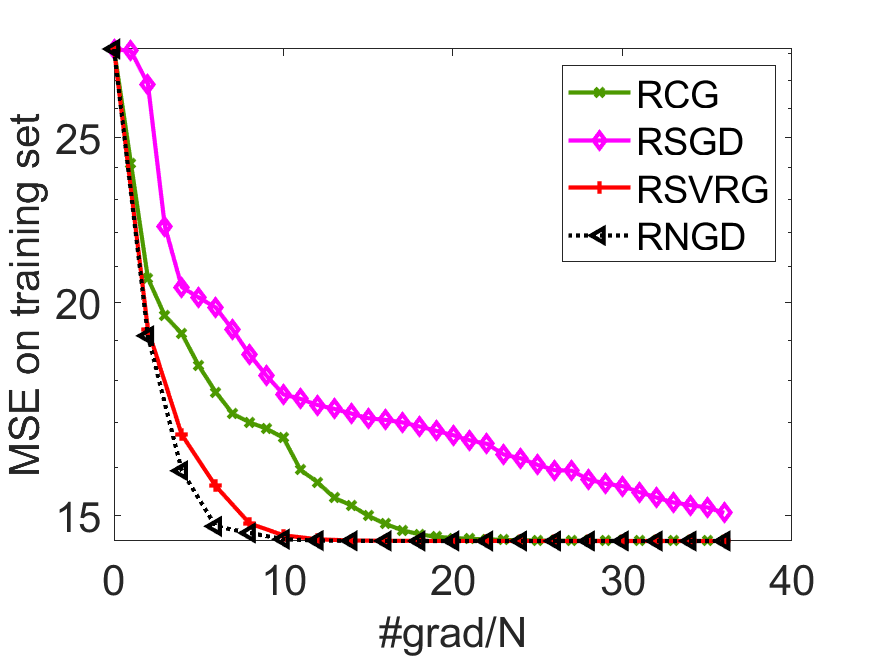
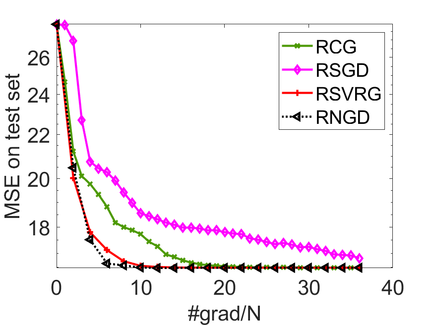
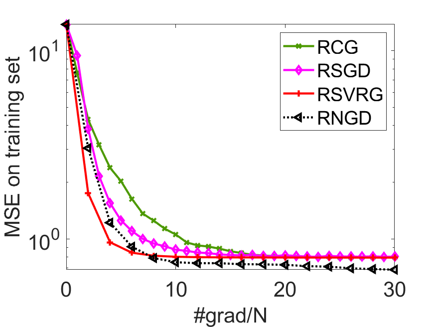
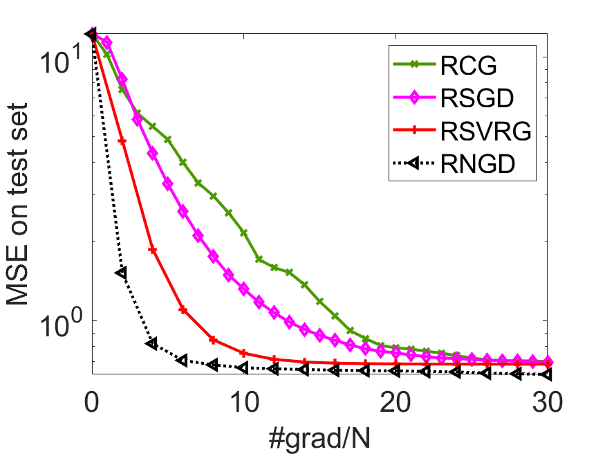
Figure 1: Numerical results for LRMC on the Jester dataset (first row) and the MovieLens-1M dataset (second row).

6.2 Low-dimension subspace learning

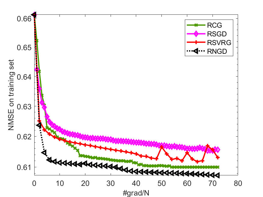
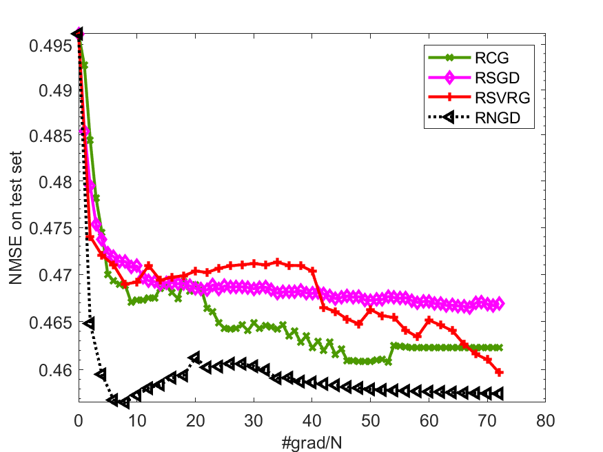
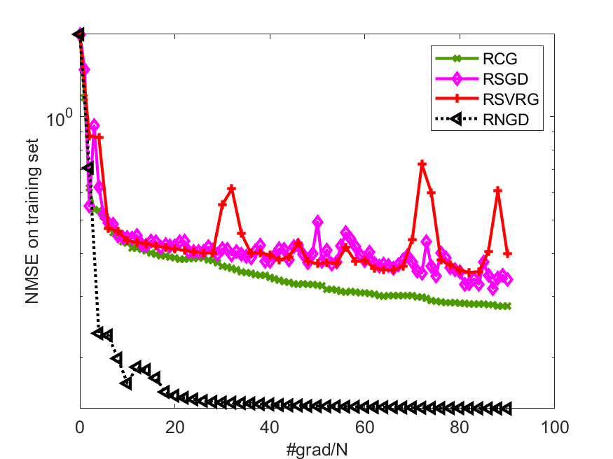
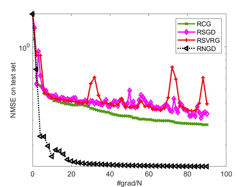
Figure 2: Numerical results for multitask learning on the $School$ dataset (first row) and the $Sarcos$ dataset (second row).

We compare our proposed RNGD with RCG, RSGD, and RSVRG on two real-world datasets: $School$ [22] and $Sarcos$ [54]. The dimension $p$ is set to be $6$ for both datasets. We choose the best step sizes for RSVRG and RSGD from the set $\{1,0.5,0.2,0.1,0.05,0.02,\ldots,10^{-8},5$ $\times 10^{-9},2\times 10^{-9},10^{-9}\}$. We use the step size 4 (resp., 1) on the $School$ (resp., Sarcos) dataset for RNGD. All the codes are implemented within the RSOpt framework and the other parameters of the algorithms are set to the default values therein.

Figure 2 reports the normalized MSE (NMSE) [39] on both datasets, which is the mean of the normalized squared error of all tasks. For both datasets, RNGD returns a point with the lowest NMSE. Especially for the $Sarcos$ dataset, a significant difference in the NMSE between RNGD and other methods is observed. Another noteworthy phenomenon is that RGD and RSVRG tend to be less efficient than RCG. This demonstrates the advantage of using the Fisher information.

6.3 Deep Learning

Batch normalization and momentum-based optimizer are standard techniques to train state-of-the-art image classification models [24, 48, 52]. We evaluate the proposed method with Kronecker-factorized approximate RFIM described in Section 4, denoted by MKFAC, on VGG16BN [52] and WRN-16-4 [61] while the benchmark datasets CIFAR-10/100 [35] are used. The detailed network structures are described in [52, 61]. In VGG16BN, batch normalization layers are added before every ReLU activation layer. Additionally, we change the number of neurons in fully connected layers from 4096 to 512 and remove the middle layer of the last three in VGG due to memory allocation problems (otherwise, one has to compute the inverse of $4096^{2}$-by-$4096^{2}$ matrices). This setting is also adopted in [17, 60].

The baseline algorithms are SGD, Adam, KFAC [38], AdamP, and SGDP [25]. The tangential projections are used to control the increase in norms of the weight parameters in AdamP and SGDP. These methods can be seen as approximate Riemannian first-order methods. We fine tune the initial learning rates of the baseline algorithms by searching in the set $\{0.5,0.2,0.1,0.05,0.02,0.01,\dots,5\times 10^{-5},2\times 10^{-5},10^{-5}\}.$ The learning rate decays in epoch 30, 60, and 90 with a decay rate $0.1$, where an epoch is defined as one cycle through the full training dataset. We choose the parameters $\beta_{1},\beta_{2}$ in Adam and AdamP from the set $\{0.9,0.99,0.999\}$. We search in the set $\{0.05,0.1,0.2,0.5,1,2\}$ to determine the damping parameter $\lambda$ used in calculating the natural direction $(F_{k}+\lambda I)^{-1}g^{k}$ and update the KFAC matrix in epoch 30, 60, and 90. The initial damping parameter of KFAC is set to $2$ in all four tasks. We set the weight decay to $5\times 10^{-4}$ for all algorithms. Each mini-batch contains 128 samples. The maximum number of epochs is set to $100$ for all algorithms. For MKFAC, we use RNGD for parameters constrained on the Grassmann manifold and SGD for the remaining parameters. Let $\eta,\eta_{g}$ denote the learning rates for the Euclidean space and Grassmann manifold, respectively. For the dataset CIFAR-10, we set $\eta_{g}=0.25$ and $\eta=0.05$ with decay rates $0.2$ and $0.1$, respectively. The weight decay is only applied to the unconstrained weights with parameter $5\times 10^{-4}$. The initial MKFAC damping parameters for WRN-16-4 and VGG16BN are set to 1 and 2 with decay rates $0.8$ and $0.5$, respectively, when the preconditioners update in epoch 30, 60, and 90. For the dataset CIFAR-100, we set $\eta_{g}=0.3$ for WRN-16-4, $\eta_{g}=0.15$ for VGG16BN, and $\eta=0.05$ for both. The learning rate $\eta_{g}$ has a decay rate $0.15$ for WRN-16-4 and $0.2$ for VGG16BN, while $\eta$ has a decay rate $0.1$ for both of them. The initial MKFAC damping parameters for VGG16BN and WRN16-4 are set to 0.5 and 1 with decay rates $0.5$ and $0.8$, respectively. Other settings are the same as KFAC.

Table 1: Classification accuracy of various networks on CIFAR-10/100 (median of five runs).

Dataset	CIFAR-10		CIFAR-100
Model	WRN-16-4	VGG16BN	WRN-16-4	VGG16BN
SGD	$93.84$	$92.88$	$74.30$	$71.79$
SGDP	$93.42$	$92.49$	$73.67$	$71.54$
Adam	$92.53$	$89.88$	$71.64$	$62.79$
AdamP	$92.55$	$91.43$	$71.23$	$58.88$
KFAC	$93.90$	$94.36$	$74.31$	$76.38$
MKFAC	94.06	94.76	74.55	77.28

Table 1 presents the comparison of the baseline and the proposed algorithms on CIFAR-10 and CIFAR-100 datasets. We list the best classification accuracy in 100 epochs, where the results are obtained from the median of 5 runs. The performance of our proposed MKFAC method is the best in all four tasks. Compared with the second-order type method KFAC, our MKFAC method reaches higher accuracy, though KFAC has a much better behavior than SGD on these tasks. Compared with the manifold geometry-based first-order algorithms SGDP and AdamP, we see that using second-order information can give better accuracy than using first-order information alone.

7 Conclusion

In this paper, we developed a novel efficient RNGD method for tackling the problem of minimizing a sum of negative log-probability losses over a manifold. Key to our development is a new notion of FIM on manifolds, which we introduced in this paper and could be of independent interest. We established the global convergence of RNGD and the local convergence rate of a deterministic version of RNGD. Our numerical results on representative machine learning applications demonstrate the efficiency and efficacy of the proposed method.

References

- [1] P.-A. Absil, R. Mahony, and R. Sepulchre, Optimization algorithms on matrix manifolds, Princeton University Press, Princeton, NJ, 2008.
- [2] P.-A. Absil, R. Mahony, and J. Trumpf, An extrinsic look at the Riemannian Hessian, in Geometric science of information, Springer, 2013, pp. 361–368.
- [3] P.-A. Absil and J. Malick, Projection-like retractions on matrix manifolds, SIAM Journal on Optimization, 22 (2012), pp. 135–158.
- [4] S.-i. Amari, Neural learning in structured parameter spaces-natural Riemannian gradient, International Conference on Neural Information Processing Systems, 9 (1996).
- [5] S.-I. Amari, Natural gradient works efficiently in learning, Neural computation, 10 (1998), pp. 251–276.
- [6] R. K. Ando, T. Zhang, and P. Bartlett, A framework for learning predictive structures from multiple tasks and unlabeled data, Journal of Machine Learning Research, 6 (2005).
- [7] R. Anil, V. Gupta, T. Koren, K. Regan, and Y. Singer, Scalable second order optimization for deep learning, arXiv:2002.09018, (2020).
- [8] J. L. Ba, J. R. Kiros, and G. E. Hinton, Layer normalization, International Conference on Neural Information Processing Systems, (2016).
- [9] A. Bahamou, D. Goldfarb, and Y. Ren, A mini-block natural gradient method for deep neural networks, arXiv:2202.04124, (2022).
- [10] G. Bécigneul and O.-E. Ganea, Riemannian adaptive optimization methods, International Conference on Learning Representations, (2019).
- [11] S. Bonnabel, Stochastic gradient descent on Riemannian manifolds, IEEE Transactions on Automatic Control, 58 (2013), pp. 2217–2229.
- [12] N. Boumal, An introduction to optimization on smooth manifolds, Available online, May, 3 (2020).
- [13] N. Boumal and P.-A. Absil, Low-rank matrix completion via preconditioned optimization on the Grassmann manifold, Linear Algebra and its Applications, 475 (2015), pp. 200–239.
- [14] N. Boumal, P.-A. Absil, and C. Cartis, Global rates of convergence for nonconvex optimization on manifolds, IMA Journal of Numerical Analysis, 39 (2018), pp. 1–33.
- [15] R. H. Byrd, S. L. Hansen, J. Nocedal, and Y. Singer, A stochastic quasi-Newton method for large-scale optimization, SIAM Journal on Optimization, 26 (2016), pp. 1008–1031.
- [16] R. Chen, M. Menickelly, and K. Scheinberg, Stochastic optimization using a trust-region method and random models, Mathematical Programming, 169 (2018), pp. 447–487.
- [17] M. Cho and J. Lee, Riemannian approach to batch normalization, International Conference on Neural Information Processing Systems, 30 (2017).
- [18] S. S. Du, X. Zhai, B. Poczos, and A. Singh, Gradient descent provably optimizes over-parameterized neural networks, International Conference on Learning Representations, (2019).
- [19] J. Duchi, E. Hazan, and Y. Singer, Adaptive subgradient methods for online learning and stochastic optimization., Journal of machine learning research, 12 (2011).
- [20] H. Flanders, Differentiation under the integral sign, The American Mathematical Monthly, 80 (1973), pp. 615–627.
- [21] D. Goldfarb, Y. Ren, and A. Bahamou, Practical quasi-Newton methods for training deep neural networks, International Conference on Neural Information Processing Systems, 33 (2020), pp. 2386–2396.
- [22] H. Goldstein, Multilevel modelling of survey data, Journal of the Royal Statistical Society. Series D (The Statistician), 40 (1991), pp. 235–244.
- [23] R. Grosse and J. Martens, A Kronecker-factored approximate Fisher matrix for convolution layers, in International Conference on Machine Learning, 2016, pp. 573–582.
- [24] K. He, X. Zhang, S. Ren, and J. Sun, Deep residual learning for image recognition, in Proceedings of the IEEE conference on computer vision and pattern recognition, 2016, pp. 770–778.
- [25] B. Heo, S. Chun, S. J. Oh, D. Han, S. Yun, G. Kim, Y. Uh, and J.-W. Ha, Adamp: Slowing down the slowdown for momentum optimizers on scale-invariant weights, International Conference on Learning Representations, (2021).
- [26] J. Hu, X. Liu, Z.-W. Wen, and Y.-X. Yuan, A brief introduction to manifold optimization, Journal of the Operations Research Society of China, 8 (2020), pp. 199–248.
- [27] S. Ioffe and C. Szegedy, Batch normalization: Accelerating deep network training by reducing internal covariate shift, in International conference on machine learning, 2015, pp. 448–456.
- [28] B. Jiang, S. Ma, A. M.-C. So, and S. Zhang, Vector transport-free SVRG with general retraction for Riemannian optimization: Complexity analysis and practical implementation, arXiv:1705.09059, (2017).
- [29] N. L. Johnson, S. Kotz, and N. Balakrishnan, Continuous univariate distributions, volume 2, vol. 289, John wiley & sons, 1995.
- [30] R. Johnson and T. Zhang, Accelerating stochastic gradient descent using predictive variance reduction, International Conference on Neural Information Processing Systems, 26 (2013), pp. 315–323.
- [31] H. Kasai, P. Jawanpuria, and B. Mishra, Riemannian adaptive stochastic gradient algorithms on matrix manifolds, in International Conference on Machine Learning, 2019, pp. 3262–3271.
- [32] H. Kasai and B. Mishra, Inexact trust-region algorithms on Riemannian manifolds., in NeurIPS, 2018, pp. 4254–4265.
- [33] H. Kasai, H. Sato, and B. Mishra, Riemannian stochastic quasi-Newton algorithm with variance reduction and its convergence analysis, in International Conference on Artificial Intelligence and Statistics, 2018, pp. 269–278.
- [34] D. P. Kingma and J. Ba, Adam: A method for stochastic optimization, International Conference for Learning Representations, (2015).
- [35] A. Krizhevsky, G. Hinton, et al., Learning multiple layers of features from tiny images, (2009).
- [36] Y. LeCun, Y. Bengio, and G. Hinton, Deep learning, Nature, 521 (2015), p. 436.
- [37] J. Martens, New insights and perspectives on the natural gradient method, The Journal of Machine Learning Research, 21 (2020), pp. 5776–5851.
- [38] J. Martens and R. Grosse, Optimizing neural networks with Kronecker-factored approximate curvature, in International conference on machine learning, 2015, pp. 2408–2417.
- [39] B. Mishra, H. Kasai, P. Jawanpuria, and A. Saroop, A Riemannian gossip approach to subspace learning on Grassmann manifold, Machine Learning, 108 (2019), pp. 1783–1803.
- [40] J. Nocedal and S. J. Wright, Numerical Optimization, Springer Series in Operations Research and Financial Engineering, Springer, New York, second ed., 2006.
- [41] L. Nurbekyan, W. Lei, and Y. Yang, Efficient natural gradient descent methods for large-scale optimization problems, arXiv:2202.06236, (2022).
- [42] Y. Ollivier, L. Arnold, A. Auger, and N. Hansen, Information-geometric optimization algorithms: A unifying picture via invariance principles, Journal of Machine Learning Research, 18 (2017), pp. 1–65.
- [43] M. Pilanci and M. J. Wainwright, Newton sketch: A near linear-time optimization algorithm with linear-quadratic convergence, SIAM Journal on Optimization, 27 (2017), pp. 205–245.
- [44] Y. Ren and D. Goldfarb, Kronecker-factored quasi-Newton methods for convolutional neural networks, arXiv:2102.06737, (2021).
- [45] H. Robbins and S. Monro, A stochastic approximation method, The Annals of Mathematical Statistics, (1951), pp. 400–407.
- [46] F. Roosta-Khorasani and M. W. Mahoney, Sub-sampled Newton methods, Mathematical Programming, 174 (2019), pp. 293–326.
- [47] T. Salimans and D. P. Kingma, Weight normalization: A simple reparameterization to accelerate training of deep neural networks, International Conference on Neural Information Processing Systems, 29 (2016), pp. 901–909.
- [48] M. Sandler, A. Howard, M. Zhu, A. Zhmoginov, and L.-C. Chen, Mobilenetv2: Inverted residuals and linear bottlenecks, in Proceedings of the IEEE conference on computer vision and pattern recognition, 2018, pp. 4510–4520.
- [49] H. Sato, H. Kasai, and B. Mishra, Riemannian stochastic variance reduced gradient algorithm with retraction and vector transport, SIAM Journal on Optimization, 29 (2019), pp. 1444–1472.
- [50] H. Sato, H. Kasai, and B. Mishra, Riemannian stochastic variance reduced gradient algorithm with retraction and vector transport, SIAM Journal on Optimization, 29 (2019), pp. 1444–1472.
- [51] N. N. Schraudolph, Fast curvature matrix-vector products for second-order gradient descent, Neural computation, 14 (2002), pp. 1723–1738.
- [52] K. Simonyan and A. Zisserman, Very deep convolutional networks for large-scale image recognition, arXiv:1409.1556, (2014).
- [53] A. M.-C. So, Non-asymptotic performance analysis of the semidefinite relaxation detector in digital communications. Preprint, 2010.
- [54] S. Vijayakumar, A. D’souza, T. Shibata, J. Conradt, and S. Schaal, Statistical learning for humanoid robots, Autonomous Robots, 12 (2002), pp. 55–69.
- [55] X. Wang and Y.-x. Yuan, Stochastic trust region methods with trust region radius depending on probabilistic models, arXiv:1904.03342, (2019).
- [56] X. Wu, S. S. Du, and R. Ward, Global convergence of adaptive gradient methods for an over-parameterized neural network, arXiv:1902.07111, (2019).
- [57] M. Yang, A. Milzarek, Z. Wen, and T. Zhang, A stochastic extra-step quasi-Newton method for nonsmooth nonconvex optimization, Mathematical Programming, (2021), pp. 1–47.
- [58] M. Yang, D. Xu, H. Chen, Z. Wen, and M. Chen, Enhance curvature information by structured stochastic quasi-Newton methods, in Proceedings of the IEEE/CVF Conference on Computer Vision and Pattern Recognition, 2021, pp. 10654–10663.
- [59] M. Yang, D. Xu, Q. Cui, Z. Wen, and P. Xu, NG+: A multi-step matrix-product natural gradient method for deep learning, arXiv:2106.07454, (2021).
- [60] M. Yang, D. Xu, Z. Wen, M. Chen, and P. Xu, Sketchy empirical natural gradient methods for deep learning, arXiv:2006.05924, (2020).
- [61] S. Zagoruyko and N. Komodakis, Wide residual networks, arXiv:1605.07146, (2016).
- [62] D. Zhang and S. D. Tajbakhsh, Riemannian stochastic variance-reduced cubic regularized Newton method, arXiv:2010.03785, (2020).
- [63] G. Zhang, J. Martens, and R. Grosse, Fast convergence of natural gradient descent for overparameterized neural networks, in International Conference on Neural Information Processing Systems, 2019, pp. 8082–8093.
- [64] H. Zhang, S. J. Reddi, and S. Sra, Riemannian SVRG: Fast stochastic optimization on Riemannian manifolds, in International Conference on Neural Information Processing Systems, 2016, pp. 4592–4600.