Parameterization of Cross-Token Relations with Relative Positional Encoding for Vision MLP

Parameterization of Cross-Token Relations with Relative Positional Encoding for Vision MLP

Abstract.

Vision multi-layer perceptrons (MLPs) have shown promising performance in computer vision tasks, and become the main competitor of CNNs and vision Transformers. They use token-mixing layers to capture cross-token interactions, as opposed to the multi-head self-attention mechanism used by Transformers. However, the heavily parameterized token-mixing layers naturally lack mechanisms to capture local information and multi-granular non-local relations, thus their discriminative power is restrained. To tackle this issue, we propose a new positional spacial gating unit (PoSGU). It exploits the attention formulations used in the classical relative positional encoding (RPE), to efficiently encode the cross-token relations for token mixing. It can successfully reduce the current quadratic parameter complexity $O(N^{2})$ of vision MLPs to $O(N)$ and $O(1)$. We experiment with two RPE mechanisms, and further propose a group-wise extension to improve their expressive power with the accomplishment of multi-granular contexts. These then serve as the key building blocks of a new type of vision MLP, referred to as PosMLP. We evaluate the effectiveness of the proposed approach by conducting thorough experiments, demonstrating an improved or comparable performance with reduced parameter complexity. For instance, for a model trained on ImageNet1K, we achieve a performance improvement from 72.14% to 74.02% and a learnable parameter reduction from $19.4M$ to $18.2M$. Code could be found at https://github.com/Zhicaiwww/PosMLP.

1. Introduction

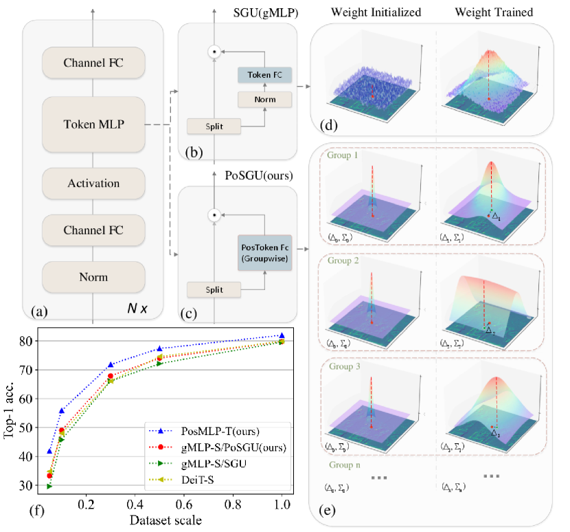
Figure 1. (a), (b) and (c) present the basic network block, the SGU used by gMLP (Liu et al., 2021a), and the proposed PoSGU in a group-wise implementation,respectively. (d) and (e) visualize the projection weights of the SGU and PoSGU,respectively. Here, the red anchor represents a query token. The rainbow distribution shows the intensity of attention logits to its surrounding tokens. (f) shows the sample efficiency results for ImageNet2012 with modified sample ratio setting per class.

In computer vision, the three types of mainstream architecture CNN, Transformer and MLP support the backbone neural network design. CNNs directly operate on 2D images, while vision transformers and MLPs convert each input image to a sequence of tokens. Subsequently, they rely on different operational approaches to extract information from the images. CNNs use convolutions to model local content patterns, and use the weight sharing mechanism to improve design efficiency (Simoncelli and Olshausen, 2001; Krizhevsky et al., 2012). To capture cross-token interaction, vision transformers use the multi-head self-attention (MHSA) mechanism, and MLPs use the token-mixing layers. As compared to CNNs, the vision transformers and MLPs are notably better at their global receptive field, i.e. MHSA and token-mixing, and have the advantage of unsaturated discriminatory power when processing hyper-scale datasets (Tolstikhin et al., 2021; Dosovitskiy et al., 2021). But they bear the weakness of requiring large-scale pre-training, e.g., having more model parameters and thus consuming more training examples, due to the weak inductive bias (Touvron et al., 2021b; Tolstikhin et al., 2021; Ding et al., 2021). Various research effort has been made to address this limitation for vision transformers, resulting in a series of new transformer design, e.g., locality-enhanced transformers (LocalViT) (Hu et al., 2019), Swin transformer (Liu et al., 2021b) and NesT transformer (Zhang et al., 2021b).

However, there is a research gap in vision MLP development, where the latest designs are still demanding in parameterization and pre-training. For instance, to improve over MLP-Mixer (Tolstikhin et al., 2021) that is the first MLP-based vision model, gMLP (Liu et al., 2021a) uses a gating mechanism and a single-token fully connected (FC) layer, referred to as the spacial gating unit (SGU), to achieve efficient aggregation of spacial information. But it results in a dramatically increased parameter number as the token number grows larger. More recently, building on the idea of token-free substitute, axial shifted MLP (AS-MLP) (Lian et al., 2021), Permute-MLP (Hou et al., 2022), Hire-MLP (Guo et al., 2021) and spatial shift MLP (s²-MLP) (Yu et al., 2022) design different spatial shift variants to simulate token interaction. As a result, they have managed to remove parameters depending on token dimensions but created extra FC layers instead. This has actually increased their parameter numbers. Additionally, their spatial shift replacement has caused a loss of intrinsic property when aggregating the global features in a token FC layer, i.e., explicit shift operation should gain global receptive field by deepening the network.

To fill in this research gap, we propose to utilize the relative positional encoding (RPE) (Shaw et al., 2018) to improve the vision MLPs, aiming at reducing the model parameterization but without sacrificing the model expressive power. Our enhanced MLP is named as PosMLP. The design is motivated by the fact that the ultimate goal of a token-mixing MLP is to model the relations across tokens (spatial pixels), why not directly parameterize the relations in an efficient way. Therefore, we make the following contributions:

• We propose a positional spacial gating unit (PoSGU) to model cross-token interactions. Its main building block is a PosToken FC layer developed based on RPE that has been proven to be efficient to encode the interaction between the key and query items in attention modelling.

• We implement two RPE mechanisms in the PoSGU. As compared to the quadratic parameter complexity $O(N^{2})$ of gMLP, the first mechanism can reduce the complexity to $O(N)$ while the later to $O(1)$.

• Additionally, we propose a group-wise extension to achieve the multi-granular spacial feature aggregation and enhance the expressive power of the RPE.

Figure 1 highlights the architecture difference between PoSGU (the GGQPE version by default, see Sec 4.1) and SGU from the gMLP that both are sharing the same basic network block design. Subgraphs (d) and (e) show that our token-mixing logits initialized in PoSGU are highly concentrated around the query token and the cross-token correlation is modeled by learned non-isotropic Gaussian distribution. After a thorough evaluation, the results show that a simple PoSGU can result in satisfactory performance with a significantly reduced parameter number, e.g. a comparable performance to the transformer-based DeiT-S (Touvron et al., 2021b) as in Figure 1 (f). For instance, for a model trained on ImageNet1K with 0.5 sample ratio, our approach can achieve a performance improvement from 72.14% to 74.02% and a parameter (learnable) reduction from $19.4M$ to $18.2M$.

2. Related Work

Vision transformers. In recent years, vision transformers have shown promising image classification results for his strong power on modeling long-range dependencies over pixels (Liu et al., 2021b; Zhang et al., 2021a; Fang et al., 2022; Cheng et al., 2018). The vision transformer (ViT) (Dosovitskiy et al., 2021) is the pilot work that extends the linguistical-style transformers on visual content modeling by treating a 2D image as a sequence of 1D tokens (patches) while remaining the vision robustness (Bhojanapalli et al., 2021). DeiT(Touvron et al., 2021b) further adopts distillation (Hinton et al., 2015) from a CNN teacher and extensive data augmentations to successfully boost the image classification performance. To be friendly to more downstream tasks like object detection and segmentation (Lin et al., 2014), PVT (Wang et al., 2021) provides the hierarchical architecture for efficient vision transformer. Swin transformer (Liu et al., 2021b) further manipulates shifted windows into the hierarchical architecture and gains notable performance improvement. To further enhance with local information, CoAtNet (Dai et al., 2021) explicitly integrates convolutional blocks into the feedforward transformer network.

Vision MLPs. MLP-like models were also developed under the premise of large-scale pre-training(Tolstikhin et al., 2021; Touvron et al., 2021a). Equipped with normalization (Ba et al., 2016) and residual connection (He et al., 2016), the architecture of stacking pure linear layers can also achieve comparable results with CNNs. However, the token mixing MLP in MLP-Mixer (Tolstikhin et al., 2021) and gMLP (Liu et al., 2021a) introduce few inductive biases and constraint the input resolution. To overcome these, bunch of works are built upon the consumption-free shift&rearrange operation, e.g. s²-MLP (Yu et al., 2022) that uses spatial shifing MLP to replace token mixing MLP, AS-MLP(Lian et al., 2021) that axially shift feature in the spacial dimension, Vision Permutator (Hou et al., 2022) that uses Permute-MLP to mix height and width information simultaneously, and Hire-MLP (Guo et al., 2021) that uses the pairwise rearrange&restore manipulations to realize local and global feature exchanging over patches. Besides, Rep-MLP (Ding et al., 2021) implemented reparameterization to merge trained convolution layers into a pure MLP network for evaluation. Different from these aforementioned methods, our PosMLP first implements positional encoding as a fully prior to explicitly model token interactions in MLP, and hence achieves better sample and parameter efficiency.

Positional Encoding. Transformer is inherently lack of sensitivity to token position, and so is MLPs. Positional encoding (PE) is a fairly mature method implemented in transformer to overcome this problem (Radford et al., 2019, 2018; Ju et al., 2020). There are commonly two kinds of positional encoding (PE) methods, i.e., absolute PE (APE) and relative PE (RPE). Sinusoidal positional encoding is the first APE implemented in vanilla transformer (Vaswani et al., 2017), aiming to introduce a prior of absolute token position distinction. RPE was first introduced to amplify the natural sensitivity of relative distance in linguistic expressions(Shaw et al., 2018; He et al., 2020; Huang et al., 2020) and late extensively adopted in vision transformers (Ke et al., 2020) which requires a strong prior of 2D displacement between pixels. Original RPE is based on a learnable relative positional embedding and thus introduces a soft positional inductive bias. CAPE (Likhomanenko et al., 2021) utilizes an enhaced APE strategy to realize the model generalization as introduced by RPE. By contrast, Quadratic Positional Encoding (QPE) (Cordonnier et al., 2019) was proposed to bring a pre-defined relative position embedding to multi-head self attention (MHSA) such that it can act like a convolutional layer. ConViT (d’Ascoli et al., 2021) integrates QPE into DeiT (Touvron et al., 2021b) and achieves a higher sample efficiency. Our work further develops Generalized QPE into a group-wise variant for vision MLPs, such that it obtains better expression ability.

3. Preliminaries

In this section, we first introduce the design of spacial gating unit (SGU) of gMLP. Next, we summarize a general representation for two representative relative positional encoding (RPE) methods, i.e., learnable relative positional encoding (LRPE) and generalized quadratic positional encoding (GQPE), which are commonly used by vision Transformers.

3.1. Spatial Gating Unit

SGU is the main building block of gMLP (Liu et al., 2021a), used to enable cross-token interactions. Let $\mathbf{X}\in\mathbb{R}^{N\times d}$ be the token representations, where $N$ and $d$ denotes the token number and embedding (channel) dimension, respectively. SGU splits the token representations into two independent parts along the dimension, denoted by $\mathbf{X}^{1}\in\mathbb{R}^{N\times\frac{d}{2}}$ and $\mathbf{X}^{2}\in\mathbb{R}^{N\times\frac{d}{2}}$. It uses a linear projection on one part to calculate a gating mask, then uses the mask to refine element-wisely the other part. Denote the refined token representations by $\mathbf{Z}\in\mathbb{R}^{N\times\frac{d}{2}}$, and it is computed by

(1) $$\mathbf{Z}=\left(\mathbf{W}\textmd{Norm}(\mathbf{X}^{1})+\bm{b}\right)\odot\mathbf{X}^{2},$$

where $\mathbf{W}\in\mathbb{R}^{N\times N}$, $\bm{b}\in\mathbb{R}^{N}$ and $\odot$ denotes the Hadamard product. $\textmd{Norm}(\cdot)$ here is the $LayerNorm$ (Ba et al., 2016). The projection matrix $\mathbf{W}$ is for feature refinement, and the gating operation encourages higher-order information interactions (Liu et al., 2021a). As shown in the SGU diagram in Figure 1(b), the operation $\tilde{\mathbf{X}}^{1}=\textmd{Norm}(\mathbf{X}^{1})$ is referred to as the Norm layer, and the operation of $\left(\mathbf{W}\tilde{\mathbf{X}}^{1}+\bm{b}\right)$ is referred to as the Token FC layer. Specifically, the Hadamard product is representing as the gating operation.

3.2. Relative Positional Encoding

Both absolute and relative positional encoding mechanisms have been widely used in vision transformers (Ke et al., 2020; Chu et al., 2021; Dong et al., 2021). We introduce only RPE since our research focus is to model the pairwise relations between tokens. The core idea of RPE is to enhance the calculation of the attention $\mathbf{A}\in\mathbb{R}^{N\times N}$ by considering the position difference between tokens. In general, the token position is marked in a square window $\left(\sqrt{N},\sqrt{N}\right)$ and therefore $\bm{\delta}$ lies in the range $\left[-\sqrt{N}+1,\sqrt{N}-1\right]\times\left[-\sqrt{N}+1,\sqrt{N}-1\right]$. A relative position is a $2$-dimensional vector $\bm{\delta}_{i,j}=\bm{p}_{j}-\bm{p}_{i}$ where $\bm{p}_{i},\bm{p}_{j}$ are the positions of the $i$th and $j$th tokens in the square window. For simplicity, we omit the head dimension (i.e., single-head). The pipeline formulation of RPE can be generalized as

(2) $$\mathbf{A}_{i,j}:= \;\textmd{Softmax}_{j}\left(\mathbf{W}_{i,j}+\mathbf{W}^{r}_{i,j}\right),$$

(3) $$\mathbf{W}^{r}_{i,j}:= \;\bm{v}\bm{r}^{\top}_{\bm{\delta}_{i,j}},$$

(4) $$\mathbf{W}_{i,j}:= \;\mathbf{Q}_{i,:}\mathbf{K}^{\top}_{j,:},$$

where $1\leq i,j\leq N$, $\mathbf{Q}$ and $\mathbf{K}$ are the query and key matrices in a transformer, and $\bm{v}\in\mathbb{R}^{D_{pos}}$ is a projection vector that aggregates the relative positional embedding $\bm{r}_{\bm{\delta}}\in\mathbb{R}^{D_{pos}}$ to obtain the attention bias. Different RPE approaches vary in the formulation of $\bm{r}_{\bm{\delta}}$ and $\mathbf{W}_{i,j}^{r}$. The two representative RPE algorithms of learnable relative positional encoding (LRPE) (Hu et al., 2018; He et al., 2017; Raffel et al., 2019) and generalized quadratic positional encoding (GQPE) (Cordonnier et al., 2019) are used in our work.

Learnable Relative Positional Encoding: LRPE simply sets $D_{pos}=1$. Consequently, both $\bm{v}$ and $\bm{r}$ in $\mathbf{W}^{r}$ collapse to a single scalar and $v$ is further set to constant 1. It constructs a learnable relative positional embedding dictionary $\bm{r}_{\bm{\delta}}^{\textmd{lrpe}}\in\mathbb{R}^{\left(2\sqrt{N}-1\right)^{2}}$ with a parameter complexity of $\mathcal{O}(N)$. Here, $\bm{\delta}$ is used as an index.

Generalized Quadratic Positional Encoding: GQPE was firstly proposed for MHSA. It mimics the function of the convolutional layer by forming a non-isotropic Gaussian distribution over the query token:

(5) $$\vspace{-0.1cm}\mathbf{A}^{\textmd{gqpe}}_{i,j} :=\textmd{Softmax}_{j}\left(-\frac{1}{2}\left(\bm{\delta}_{i,j}-\bm{\Delta}\right)\mathbf{\Sigma}^{-1}\left(\bm{\delta}_{i,j}-\bm{\Delta}\right)^{\top}\right),$$

(6) $$=\textmd{Softmax}_{j}\left(\bm{v}\bm{r}^{\top}_{\bm{\delta}_{i,j}}\right).$$

To obtain such a distribution pattern, the learnable vector $\bm{v}$ is parameterized by a center of attention $\mathbf{\Delta}\in\mathbb{R}^{2}$ and a positive semi-definite covariance matrix $\mathbf{\Sigma}=\mathbf{\Gamma}\mathbf{\Gamma}^{\top}$, where $\mathbf{\Gamma}\in\mathbb{R}^{2\times 2}$. In total, there are 6 parameters. The parameter complexity is $\mathcal{O}(1)$. Subsequently,

(7) $$\bm{v}^{\textmd{gqpe}}= \left[\left(\mathbf{\Sigma}^{-1}\mathbf{\Delta}\right)_{1},\left(\mathbf{\Sigma}^{-1}\mathbf{\Delta}\right)_{2},-\frac{1}{2}\mathbf{\Sigma}_{1,1}^{-1},-\frac{1}{2}\mathbf{\Sigma}^{-1}_{2,2},-\mathbf{\Sigma}^{-1}_{1,2}\right]^{\top},$$

(8) $$\bm{r}^{\textmd{gqpe}}_{\bm{\delta}}= \left[\bm{\delta}_{x},\bm{\delta}_{y},\bm{\delta}^{2}_{x},\bm{\delta}^{2}_{y},\bm{\delta}_{x}\bm{\delta}_{y}\right]^{\top}.$$

The relative positions $\bm{r}_{\bm{\delta}}$ of GQPE is not learnable and is determined only by the relative position $\bm{\delta}=(\bm{\delta}_{x},\bm{\delta}_{y})$. For the attention map of the $i$-th query token, $\bm{\Delta}$ controls the displacement of the distribution center relative to the position $\bm{p}_{i}$, and $\mathbf{\Sigma}$ controls the distribution function where it is semi-definite positive such that the attention maximum will always be guaranteed at $\bm{\Delta}=\bm{\delta}$.

Since GQPE introduces a hard relative position prior, we view it as a hard RPE similar to the hard inductive bias introduced by CNN (d’Ascoli et al., 2021).

4. Positional MLP (PosMLP)

The Token FC layer used in classical vision MLPs bears the weakness of poor inductive biases (Tolstikhin et al., 2021) and has a quadratic parameter complexity $\mathcal{O}(N^{2})$ with respect to the number of tokens. We propose to transfer the idea of RPE used in attention formulation for transformers to formulate the projection matrix in SGU. This introduces extra positional information in the Token FC layer of SGU. Therefore, we name the improved SGU as PoSGU, and the improved vision MLP with such new units as PosMLP. This proposal can successfully reduce the parameter complexity of token-mixing to only $\mathcal{O}(N)$ or $\mathcal{O}(1)$ without sacrificing the model performance.

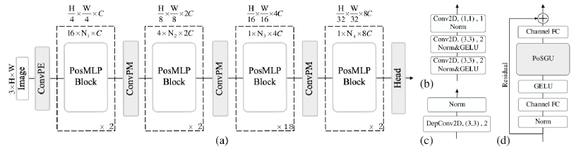
Figure 2. The proposed PosMLP: (a) Overall architecture; (b) Convolutional Patch Embedding block; (c) Convolutional Patch Merging block; (d) Architecture of PosMLP block with PoSGU.

4.1. Positional SGU (PoSGU)

Starting from the classical SGU operation $\left(\mathbf{W}\tilde{\mathbf{X}}^{1}+\bm{b}\right)\odot\mathbf{X}^{2}$ as explained in preliminaries, we omit $\bm{b}$ since the bias term $\bm{b}$ operates independently on $\mathbf{X}^{2}$. We will also discuss this in the experiment later. This results in $\left(\mathbf{W}\tilde{\mathbf{X}}^{1}\right)\odot\mathbf{X}^{2}$, based on which we propose the base formulation of PoSGU, as

(9) $$\vspace{-0.1cm}\mathbf{Z}=\left(\left(\mathbf{W}+\mathbf{W}^{r}\right)\tilde{\mathbf{X}}^{1}\right)\odot\mathbf{X}^{2},$$

where $\mathbf{W}^{r}$ encodes the positional information and is formulated by taking advantage of the attention weight formulation in Eq. (3).

LRPE-based PoSGU: When following the LRPE principal, $\mathbf{W}$ can be simply modified to $\mathbf{W}+\bm{r}^{\textmd{lrpe}}_{\bm{\delta}}$ in order to cooperate the positional information. This results in

(10) $$\mathbf{Z}^{\textmd{lrpe-M}}=\left(\mathbf{W}+\bm{r}^{\textmd{lrpe}}_{\bm{\delta}}\right)\textmd{Norm}(\mathbf{X}^{1})\odot\mathbf{X}^{2},$$

where the relative positional encoding matrix $\mathbf{W}^{r}$ can be calculated by $\bm{r}^{\textmd{lrpe}}_{\bm{\delta}}$. It is worth to mention that we remove the Softmax operation, due to its co-occurrence with the LayerNorm operation will cause a significant performance drop. Note that our LRPE-M shares a similar spirit with the bias mode of the iRPE (Wu et al., 2021). Through empirical observations, e.g., in the Figure S7 where we visualized each projection matrix and plotted the logits intensity corresponding to the query token. We notice that the positional embedding $\bm{r}^{\textmd{lrpe}}_{\bm{\delta}}$ can learn more localities and can reserve partially its non-locality in deeper layers, while the effect of W is weak and sometimes it can be redundant. Therefore, we remove W and this results in

(11) $$\mathbf{Z}^{\textmd{lrpe}}=\bm{r}^{\textmd{lrpe}}_{\bm{\delta}}\textmd{Norm}(\mathbf{X}^{1})\odot\mathbf{X}^{2}.$$

More importantly, this revised operation significantly decreases the parameter complexity.

GQPE-based Group-wise PoSGU: An alternative is to follow the GQPE principal. The particular benefit is its extremely low parameter complexity $\mathcal{O}(1)$. Meanwhile, to increase the model expressive power, we enhance it with a group-wise strategy (Hao et al., 2022). Inspired by the multi-head operation used by transformers and the group convolution operation used by CNNs, we find it beneficial to split further the token embeddings along their channel dimension, and then project different splits with different learnable vectors. Specifically, after splitting the token representations $\mathbf{X}\in\mathbb{R}^{N\times d}$ into $\mathbf{X}^{1}\in\mathbb{R}^{N\times\frac{d}{2}}$ and $\mathbf{X}^{2}\in\mathbb{R}^{N\times\frac{d}{2}}$, we further split each into $s$ feature groups: $\left\{\mathbf{X}^{1}_{1},\mathbf{X}^{1}_{2},\cdots,\mathbf{X}^{1}_{s}\right\}\in\mathbb{R}^{N\times\frac{d}{2s}}$ and $\left\{\mathbf{X}^{2}_{1},\mathbf{X}^{2}_{2},\cdots,\mathbf{X}^{2}_{s}\right\}\in\mathbb{R}^{N\times\frac{d}{2s}}$. Following the idea of Eq. ( 6), we have, for the $s$-th group,

(12) $$\mathbf{Z}^{\textmd{gqpe}}_{s}=\mathbf{A}^{\textmd{gqpe}}_{s}\mathbf{X}^{1}_{s}\odot\mathbf{X}^{2}_{s},$$

(13) $$\mathbf{A}^{\textmd{gqpe}}_{s,i,j}=\textmd{Softmax}_{j}\left(\bm{v}^{\textmd{gqpe}}_{s}\bm{r}^{\textmd{gqpe}^{\top}}_{\bm{\delta}_{i,j}}\right).$$

Then, we concatenate all the group representations:

(14) $$\mathbf{Z}^{\textmd{gqpe}}=\textmd{Concat}\left(\mathbf{Z}^{\textmd{gqpe}}_{2},\mathbf{Z}^{\textmd{gqpe}}_{2},\cdots,\mathbf{Z}^{\textmd{gqpe}}_{s}\right).$$

The $s$ groups share the same relative positional embedding $\bm{r}^{\textmd{gqpe}}_{\bm{\delta}}$ but different learnable vector $\bm{v}^{\textmd{gqpe}}_{s}$. We omit the Norm layer here since the co-occurrence of Norm and Softmax will cause a performance drop (check Section 3) The calculation builds on multiple pairwise shift attention centers $\{\mathbf{\Delta}_{1},\mathbf{\Delta}_{2},\cdots,\mathbf{\Delta}_{s}\}$ and covariance matrices $\{\mathbf{\Sigma}_{1},\mathbf{\Sigma}_{2},\cdots,\mathbf{\Sigma}_{s}\}$. A {shift attention center, covariance matix} pair can lead to a particular granularity of contextual information (local or non-local, mostly determined by the form of $\mathbf{\Sigma}$ as Sec.5.3 shows). Therefore, this group-wise operation can improve over the original GQPE, being able to flexibly attend multiple granularities of contextual information in a single layer. It can potentially enrich the captured spatial information and ease the training (see Section 5.1 for results). It is worth to mention that this group-wise strategy can be easily transferred to the LRPE mechanism, resulting in the GLRPE. We provide a simple illustration in Figure S6, to highlight the difference between the classical Token FC and the proposed token-mixing methods based on LRPE and GQPE.PE and GQPE-based token-mixing methods in this section, see Figure S6.

4.2. PosMLP Architecture

We propose a new vision MLP model PosMLP, of which each basic block is integrated with our proposed PoSGU. For illustration purpose, Figure 2 depicts the model architecture of a tiny PosMLP, which is mainly composed of the convolutional downsampling (ConvPE + ConvPM) and PosMLP block.

Convolutional Patch Embedding (ConvPE): The ConvPE block receives the input of a raw image with a shape $H\times W\times 3$ and outputs the patch embeddings. The module shares the similar spirit as (Xiao et al., 2021) in transformers, which stacks several convolutional layers to improve the stability of the model training. In our implementation, as shown in Figure 2(b), the block contains three consecutive convolutional layers. The use of convolutions adequately encodes the local information in visual modelling. Finally, this operation results in a $\frac{H}{4}\times\frac{W}{4}\times C$ feature map.

Convolutional Patch Merging (ConvPM): Inspired by Nest Transformer (Zhang et al., 2021b) that uses the “Convolution+Maxpooling” to perform the spacial downsampling with the ratio of $2$ and a channel expansion ratio of $2$, we adopt a depth-wise convolution with stride 2 to achieve a similar effect.

Positional encoding MLP: The architecture of a PosMLP block is illustrated in Figure 2 (d). It has a similar structure to gMLP, but replaces the SGU with the proposed PoSGU. Thanks to the RPE mechanisms, it is able to model both local and non-local information, thus can entirely replace the token-mixing operations in the original vision MLPs.

Windows Partitioning: To be fed into a PosMLP block, the image input is blocked into multiple non-overlapping windows of the given size and sequenced as tokens. Then it is reshaped back to a feature map for performing convolutional downsampling. In our implementation, we assign different window sizes to different stages by considering the feature map size, i.e., $14\times 14$ for the first three stages “Stage 1,2,3”, resulting in the $14\times 14=196$ (i.e., $N=196$) tokens (pixels) and the corresponding $16,4,1$ feature windows respectively, and $7\times 7$ for the “Stage 4” and $49$ tokens with $1$ feature windows. The most obvious advantage of using a windows-based structure is that it can significantly reduce the computational cost (Liu et al., 2021b) and realize parameters sharing among windows.

Architecture Variant: We build our model variants similar to the classic works like Swin-Transformer, including three 4-stages PosMLP-T/S/B where the capital letters “T, S, B” refer to “Tiny, Small, Base” models. The main difference between PosMLP-T, PosMLP-S, and PosMLP-B lies in the model size which is led by separately setting the feature channel $C$ to 96, 128, and 192. All the other hyper-parameters such as window size, group numbrt $s$, and channel expansion ratio $\gamma$ are kept the same among the three variants. Table S11 lists the detailed settings of these model architectures.

5. Experiments

In this section, we report the experimental results evaluated on ImageNet1K and COCO2017. We also conduct an ablation study to validate the impacts of hyperparameters and key components of our model. Moreover, we also give the visualized results to clearly observe the functions of the introduced positional encoding in spatial relation modeling. All the experiments are conducted on 4/8$\times$ 3090 GPUs.

5.1. RPE in Vision MLP

We firstly give a comprehensive comparison for the proposed PoSGU modules. Both gMLP and our PosMLP are employed as backbone architectures. Table 1 lists their model complexity w.r.t token-mixing, extra FLOPs and top-1 accuracy by performing image classification on ImageNet1K^0.5. Note that the extra FLOPs means the additional computational cost of gating unit compared with base SGU.

Table 1. Comparison of different RPE module variants with respect to mode complexity, extra FLOPs and top-1 accuracy using gMLP and our PosMLP as backbones. SGU refers to the spatial gating unit proposed by gMLP. PoSGU refers to our proposed positional spatial gating unit. PoSGU has four variants, i.e., LRPE-M, LRPE, and two corresponding group-wise modules GLRPE and GGQPE.

Model	Module		Token-mixing complexity	Extra FLOPs	Top-1 acc.
gMLP	SGU		$\mathcal{O}(N^{2})$	✗	72.14
	PoSGU	LRPE-M	$\mathcal{O}(N^{2})$	$\mathcal{O}(N^{2})$	73.96(+1.82)
		LRPE	$\mathcal{O}(N)$	$\mathcal{O}(N^{2})$	72.44(+0.30)
		GLRPE	$\mathcal{O}(N)$	$\mathcal{O}(sN^{2})$	74.56(+2.42)
		GGQPE	$\mathcal{O}(1)$	$\mathcal{O}(sN^{2})$	74.02(+1.88)
PosMLP	SGU		$\mathcal{O}(N^{2})$	✗	76.33
	PoSGU	LRPE-M	$\mathcal{O}(N^{2})$	$\mathcal{O}(N^{2})$	76.95(+0.62)
		LRPE	$\mathcal{O}(N)$	$\mathcal{O}(N^{2})$	76.93(+0.60)
		GLRPE	$\mathcal{O}(N)$	$\mathcal{O}(sN^{2})$	$\mathbf{77.41(+1.08)}$
		GGQPE	$\mathcal{O}(1)$	$\mathcal{O}(sN^{2})$	77.40(+1.07)

Observation and analysis. As shown in this table, the proposed PoSGU modules consistently outperform SGU regardless of backbones. This provides a strong proof for the feasibility of the idea of manually parameterizing cross-token correlation. Specifically, LRPE, which is a simplified LRPE-M by removing the Token FC weights $\mathbf{W}$ in Eq. (9), has almost the same top-1 accuracy (76.93 vs. 76.95 of LRPE-M for PosMLP) but significantly reduces the model complexity from $\mathcal{O}(N^{2})$ to $\mathcal{O}(N)$. Moreover, the group-wise RPE versions GLRPE and GGQPE, which further emphasizes the multiple granularities of token contexts, achieve better performance than the non-group-wise counterparts. Finally, by considering the parameter efficiency, we choose GGQPE with only $\mathcal{O}(1)$ parameter complexity as the instantiation of our PoSGU. It is worth noting that the extra FLOPs of LRPE comes from the assignment operation while GQPE has an extra cost of Multiply-Add cumulation (MACs). However, as analyzed in Appendix, the extra FLOPs incurred by GGQPE is negligible compared with the model architecture block that has an $\mathcal{O}(rmdN^{2})$ ($rmd>>s$, $s$ denotes the group number). Thus, for better illustration of direct parameterization of cross-token relation, we use GGQPE as our defalut setting for our PosMLP.

Table 2. Performance comparison of PosMLP variants with the state-of-the-arts such as CNNs, vision transformers and vision MLPs on ImageNet1K dataset.

Method	Input Size	#Param.	FLOPs	Top-1 Acc.
Tiny Models
RegNetY-4G (Radosavovic et al., 2020)	$224^{2}$	21M	4.0G	80.0
Swin-T (Liu et al., 2021b)	$224^{2}$	29M	4.5G	81.3
Nest-T (Zhang et al., 2021b)	$224^{2}$	17M	5.8G	81.5
gMLP-S (Liu et al., 2021a)	$224^{2}$	20M	4.5G	79.6
Hire-MLP-S (Guo et al., 2021)	$224^{2}$	33M	4.2G	81.8
ViP-Small/7 (Hou et al., 2022)	$224^{2}$	25M	6.9G	81.5
PosMLP-T	$224^{2}$	21M	5.2G	82.1
PosMLP-T	$384^{2}$	21M	17.7G	83.0
Small Models
RegNetY-8G (Radosavovic et al., 2020)	$224^{2}$	39M	8.0G	81.7
Swin-S (Liu et al., 2021b)	$224^{2}$	50M	8.7G	83.0
Nest-S (Zhang et al., 2021b)	$224^{2}$	38M	10.4G	83.3
Mixer-B/16 (Tolstikhin et al., 2021)	$224^{2}$	59M	11.7G	76.4
S2-MLP-deep (Yu et al., 2022)	$224^{2}$	51M	9.7G	80.7
ViP-Medium/7 (Hou et al., 2022)	$224^{2}$	55M	16.3G	82.7
Hire-MLP-B (Guo et al., 2021)	$224^{2}$	58M	8.1G	83.1
AS-MLP-S(Lian et al., 2021)	$224^{2}$	50M	8.5G	83.1
PosMLP-S	$224^{2}$	37M	8.7G	83.0
Base Models
RegNetY-16G (Radosavovic et al., 2020)	$224^{2}$	84M	16.0G	82.9
Swin-B (Liu et al., 2021b)	$224^{2}$	88M	15.4G	83.3
Nest-B (Zhang et al., 2021b)	$224^{2}$	68M	17.9G	83.8
gMLP-B (Liu et al., 2021a)	$224^{2}$	73M	15.8G	81.6
ViP-Large/7 (Hou et al., 2022)	$224^{2}$	88M	24.3G	83.2
Hire-MLP-L (Guo et al., 2021)	$224^{2}$	96M	13.5G	83.4
PosMLP-B	$224^{2}$	82M	18.6G	83.6

5.2. Image Classification

Dataset and implementation. The image classification is benchmarked on the popular ImageNet1K (Deng et al., 2009) dataset. The training/validation partitioning follows the official protocol, where $\sim$1.2M images are for training and 50K images are for validation under 1K semantic categories. The top-1 accuracy (%) is reported for performance comparison. In the training, we adopt the same data augmentations used in DeiT (Touvron et al., 2021b), including RandAugment (Cubuk et al., 2020), Mixup (Zhang et al., 2017), Cutmix (Yun et al., 2019), random erasing (Zhong et al., 2020) and stochastic depth (Huang et al., 2016). Exponential moving average (EMA) (Polyak and Juditsky, 1992) is also used for training acceleration. We train the model for 300 epochs with batch-size 120 per GPU and the cosine learning rate schedule where the initial value is set to $1\times 10^{-3}$ and minimal value is of $1\times 10^{-5}$. The AdamW (Loshchilov and Hutter, 2017) optimizer with the momentum of 0.9 and weight decay of 0.067 is adopted. Inference is performed on a single $224\times 224$ center crop using the validation set.

Results. We compare our PosMLPs with current SOTAs on ImageNet1K, including the CNN-based ResNetY models, Transformer-based Nest and Swin models, and other vision MLPs, like gMLP and AS-MLP. Table 2 reports their performance comparison regarding parameters, computations (FLOPs) and top-1 accuracies.

Amongst tiny models, our PosMLP-T achieves the 82.1% top-1 accuracy, which is better than the results of CNN-based and Transformer-based, i.e., ResNetY-4G, Nest-T, and Swin-T. Benefiting from the hierarchical structure and replacing the vanilla Token FC layer with RPE based token-mixing layer, PosMLP-T requires fewer parameters and performed well on the tiny version. While under the small and base settings, our PosMLP still exhibits its strong competitiveness. Considering the model complexity, our PosMLP-S is more efficient than Swin-S (parameters: 37M vs 50M; FLOPs: 8.7G vs 8.7G). Compared to its mostly related gMLP, PosMLP variants consistently outperform the gMLP counterparts. For example, PosMLP-B outperforms gMLP-B by a margin of 2.0%, which in a sense demonstrates the effectiveness of our implements in MLPs.

5.3. Ablation Study

In this section, we separately study the impacts of the model components, PoSGU variants, feature group number $s$ and window size. All the ablation study experiments are based on the tiny version of PosMLP and conducted on the $\text{ImageNet1K}^{0.5}$.

Table 3. Comparison with different model components.

Model	#Param.	Flops	Top-1 acc.	Top-5 acc.
gMLP (original)	19.4M	4.42G	72.18	90.52
gMLP+GGQPE	18.2M	4.45G	74.02	92.00
gMLP+ConvLHS	21.8M	5.10G	76.33	93.07
gMLP+ConvLHS+GGQPE	20.9M	5.21G	77.40	93.58

Model components The key components in PosMLP can be generalized in twos: the convolution-linked hierarchical structure (ConvLHS) and the PoSGU components. ConvLHS composes the window-based architecture and convolutional operations (ConvPE + ConvPM) to realize efficient parameter sharing and local information modeling. As shown in Table 3, we first perform the comparison between the original gMLP and the gMLP with the proposed ConvLHS. It can be found that gMLP+ConvLHS significantly improves gMLP by a large margin of $76.33-72.18=4.15$. Secondly, we directly replace the Token FC layers of gMLP with the proposed group-wise PosToken FC and observe 1.84 percentage points of performance improvement with fewer parameters and negligible extra FLOPs (we assign $s=8$ for all layers), which echoes our statement that Token FC can be replaced with positional encoding for more efficient token mixing. Finally, the combination of GGQPE and ConvLHS results in the highest performance of 77.40.

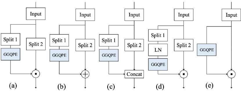
PoSGU	(a)	(b)	(c)	(d)	(e)
Top-1 acc.	$\mathbf{77.40^{*}}$	76.97	76.98	76.95	75.49

Figure 3. PoSGU variants. (a) Standard; (b) Element-wise Addition; (c) Concat; (d) LayerNorm; (e) NonSplit. ‘*’ denotes our defalut settings for PosMLP

PoSGU configurations The proposed PoSGU works in a gating manner as gMLP that splits the token embedding tensor into two parts. We study several potential configurations of PoSGU to verify the rationality of the design. Figure 8 illustrates the studied PoSGU configurations, including Element-wise Addition, Concat, LayerNorm and NonSplit variants, as well as their corresponding classification performances. Firstly, when replacing the gating operation with element-wise addition (subfigure-(b)) and channel concatenation (subfigure-(c)), we observe that performances degrade. This indicate the effectiveness of the gating operation. Secondly, when additionally adding a LayerNorm before the GGQPE (subfigure-(d)), there is also a performance degradation (77.40$\rightarrow$76.95). The potential reason could be that the Softmax used by GGQPE (see Eq. (13)) contribute to normalized token-mixed information, and extra LayerNorm will break the feature homogeneity for two splits. Finally, we empirically omit the channel splitting operation (subfigure-(e)) and find the same trend observed by gMLP that channel splitting is more effective (75.49 vs. 77.40).

Table 4. Comparison with different group numbers $s$.

$s$ each stage	Top-1 acc.	Top-5 acc.
$(1,1,1,1)$	76.70	93.02
$(4,4,4,4)$	76.87	93.40
$(4,8,16,32)$	77.10	93.24
$(32,32,32,32)$	77.02	93.14
$(8,16,32,64)^{*}$	$\mathbf{77.40}^{*}$	$\mathbf{93.58}^{*}$

Group number $s$. We compare different settings of group number $s$, which is introduced for group operation in the proposed PosToken FC module (Here we inplemented on GGQPE design), in Table 4. We observe that using group operation (76.70$\rightarrow$76.87$\rightarrow$77.02) and hierarchically increasing it (76.87$\rightarrow$77.10$\rightarrow$77.40) in each stage can significantly improve the performance. By jointly considering the channel dimensions in different stages and the performance, we finally set $s=8\times StageID$ for each stage, leading to $(8,16,32,64)$ for stages 1/2/3/4.

Table 5. Comparison using different window sizes $(k,k)$.

Win size ( $1_{th}$ stage)	#param.	FLOPs	Top-1 acc.	Top-5 acc.
$28\times 28$	20.8M	5.95G	77.81	93.91
$14\times 14^{*}$	20.8M	5.21G	$77.40^{*}$	$93.58^{*}$
$7\times 7$	20.8M	5.01G	76.98	93.45

window size. The window size decides the number of tokens $N$ in a PosMLP block. We compare three settings in the first stage, i.e., $7\times 7$, $14\times 14$ and $28\times 28$. From Table 5, it can be found that larger window size leads to monotonic performance increasing and also dramatically raises the FLOPs. To consider the trade-off between performance and efficiency, we set the patch window size as $14\times 14$ for all model variants.

Table 6. Ablation study of changing the property of covariance matrices $\bm{\tilde{}}{\Sigma}$ and whether freeze $\bm{\Delta}$ or not.

$\mathbf{\Sigma}$ form	$\alpha\mathbf{I}$	$\bm{\Gamma}$	$\bm{\Gamma}\bm{\Gamma}^{\top}$	$\bm{\Gamma}\bm{\Gamma}^{\top}$
$\mathbf{\Delta}$ freezed	✓	✓	✓	✗
Top-1 acc.	76.49	77.61	$77.40^{*}$	77.20

$\mathbf{\Sigma}$ and $\mathbf{\Delta}$ terms in GGQPE. Recall that the positional weight $\mathbf{W}^{\textmd{gqpe}}$ in Eq. (13) is determined by two terms: covariance matrix $\mathbf{\Sigma}$ and shift attention center $\mathbf{\Delta}$. Firstly, we investigate three different implementations for the covariance matrix $\mathbf{\Sigma}$, i.e., $\mathbf{\Sigma}=\alpha\mathbf{I}$ where $\mathbf{I}$ denotes the identity matrix, $\mathbf{\Sigma}=\mathbf{\Gamma}$ and the standard $\mathbf{\Sigma}=\mathbf{\Gamma}\mathbf{\Gamma}^{\top}$. Specifically, $\mathbf{\Sigma}=\alpha\mathbf{I}$, which is known as Quadratic Encoding (Cordonnier et al., 2019), only forms isotropic Gaussian distributions. By contrast, both $\mathbf{\Sigma}=\mathbf{\Gamma}$ and $\mathbf{\Sigma}=\mathbf{\Gamma}\mathbf{\Gamma}^{\top}$ can learn non-isotropic Gaussian distributions over tokens. The positive semi-definite matrix $\mathbf{\Gamma}\mathbf{\Gamma}^{\top}$ makes the attention weights maximized at the learned shift attention center $\mathbf{\Delta}$, while under $\mathbf{\Sigma}=\mathbf{\Gamma}$ this will not be guaranteed any more. Among the three settings, as shown in Table 6, $\mathbf{\Sigma}=\mathbf{\Gamma}$ and $\mathbf{\Sigma}=\mathbf{\Gamma}\mathbf{\Gamma}^{\top}$ can significantly outperform $\mathbf{\Sigma}=\alpha\mathbf{I}$, which demonstrates the superior of non-isotropic Gaussian distribution in attention learning. The three attention maps also visually give cues that $\mathbf{\Sigma}=\mathbf{\Gamma}$ and $\mathbf{\Sigma}=\mathbf{\Gamma}\mathbf{\Gamma}^{\top}$ successfully learn flexible local&non-local patterns, whereas the $\mathbf{\Sigma}=\alpha\mathbf{I}$ only learn a relative local information, as shown in Figure 4. For the deep layers in $\mathbf{\Sigma}=\mathbf{\Gamma}\mathbf{\Gamma}^{\top}$ same groups learn a global average pool attention map, potently supporting our original intention of preserving the non-localilty of MLPs. Secondly, since a learnable $\mathbf{\Delta}$ can lead to floating shift attention center, we thus ablate on what if freezing $\mathbf{\Delta}=(0,0)$ which meats the shifted attention center is fixed to the anchor pixel itself. As shown in the table, the limited displacement flexibility causes a certain degree of but not fatal degradation.

Table 7. Ablation study on the relationship between bias term in Eq.(15) and absolute positional encoding (APE).

Bias $\bm{b}$	✗	✗	✓	✓
APE	✗	✓	✗	✓
Top-1 acc.	76.8	77.3	$\mathbf{77.4}^{*}$	77.3

Table 8. Performance comparison with state-of-the-arts on object detection using COCO2017 dataset.

Backbone	#Param.	Mask R-CNN $1\times$						#Param.	RetinaNet $1\times$
		AP	$\text{AP}_{50}$	$\text{AP}_{75}$	$\text{AP}^{\text{m}}$	$\text{AP}^{\text{m}}_{50}$	$\text{AP}^{\text{m}}_{75}$		AP	$\text{AP}_{50}$	$\text{AP}_{75}$	$\text{AP}_{S}$	$\text{AP}_{M}$	$\text{AP}_{L}$
ResNet50(He et al., 2016)	44.2M	38.0	58.6	41.4	34.4	55.1	36.7	37.7M	36.3	55.3	38.6	19.3	40.0	48.8
PVT-Small(Wang et al., 2021)	44.1M	40.4	62.9	43.8	37.8	60.1	40.3	34.2M	40.4	61.3	43.0	25.0	42.9	55.7
CycleMLP-B2(Chen et al., 2022)	46.5M	41.7	63.6	45.8	38.2	60.4	41.0	36.5M	40.9	61.8	43.4	23.4	44.7	53.4
PosMLP-T(ours)	40.5M	41.6	64.1	45.6	38.4	61.1	41.0	31.1M	41.9	63.2	44.7	25.1	45.7	55.6
ResNet101(He et al., 2016)	63.2M	40.4	61.1	44.2	36.4	57.7	38.8	56.7M	38.5	57.8	41.2	21.4	42.6	51.1
PVT-Medium(Wang et al., 2021)	63.9M	42.0	64.4	45.6	39.0	61.6	42.1	53.9M	41.9	63.1	44.3	25.0	44.9	57.6
CycleMLP-B3(Chen et al., 2022)	58.0M	43.4	65.0	47.7	39.5	62.0	42.4	48.1M	42.5	63.2	45.3	25.2	45.5	56.2
PosMLP-S(ours)	56.1M	43.2	65.5	47.4	39.4	62.5	42.1	47.3M	42.4	63.6	45.1	26.5	45.7	56.3

5.4. Bias May Reveal the Absolute Positional Information

The proposed GGQPE explicitly learns the relative positional relation between a pair of tokens/pixels. Here we rewrite Eq. (12) with the presence of the bias term $b\in\mathbb{R}^{N\times 1}$. The bias $b$ is an feature agnostic term and can assign an offset value to each pixel/token at the $\sqrt{N}\times\sqrt{N}$ feature map.

(15) $$\vspace{-0.05cm}\mathbf{Z}^{\textmd{gqpe}^{s}}=(\mathbf{W}^{\textmd{gqpe}^{s}}\mathbf{X}^{1}_{s}+\bm{b})\odot\mathbf{X}^{2}_{s}.$$

So far, we still have the question that whether GGQPE can capture absolute positional information of pixels and how important the absolute position is to PosMLP. To answer it, we purposefully add the absolute position embedding to the tokens following ViT (Dosovitskiy et al., 2021), that is, element-wisely adding a learnable parameter to each element of the token embedding before the first stage, resulting in a $\sqrt{N}\times\sqrt{N}\times C$ learnable matrix. Meanwhile, we also remove the bias term $\bm{b}$ in Eq. (15) so that the GGQPE focuses entirely on the relative positional encoding. Table 8 shows the performance changes of PosMLP w/ and w/o $\bm{b}$ and absolute position encoding (APE). It can be found that (1) PosMLP w/o $\bm{b}$ underperforms PosMLP w/ APE by 0.5 percent (76.8 vs 77.3), (2) PosMLP w/ $\bm{b}$ and PosMLP w/ APE have almost the same results (77.4 and 77.3), and (3) PosMLP w/ both $\bm{b}$ and APE does not obtain any performance gain. Based on these observations, we speculate that (1) the absolute position encoding is indeed essential for our PosMLP when modeling images and (2) the bias term $\bm{b}$ in GGQPE can achieve similar function with APE which explains why our PosMLP does not need any extra absolute positions. As shown in Figure 5, we plot the logits intensity of bias $\bm{b}$ of SGU and PoSGU, respectively. We observe that the center area of an image generally has high bias values in the most stages of PoSGU, which is reasonable as the most of the informative objects locate at the center area in the ImageNet dataset.

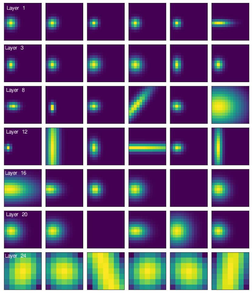
(a) $\mathbf{\Sigma}=\mathbf{\Gamma}\mathbf{\Gamma}^{\top}$

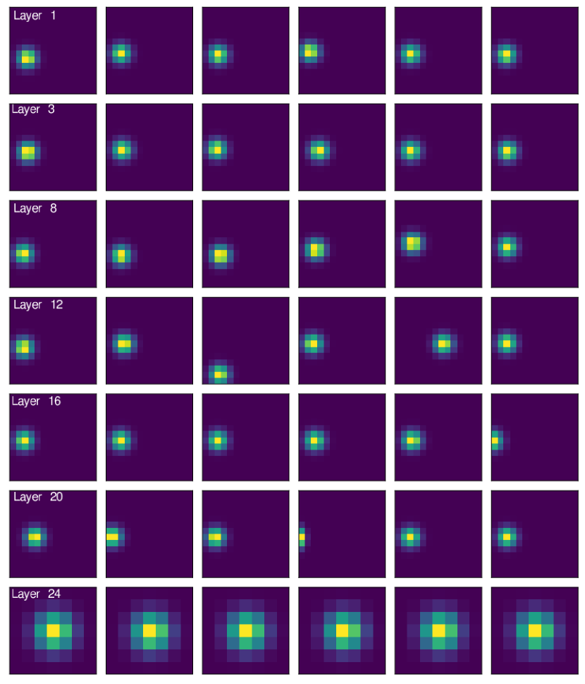
(b) $\mathbf{\Sigma}=\alpha\mathbf{I}$

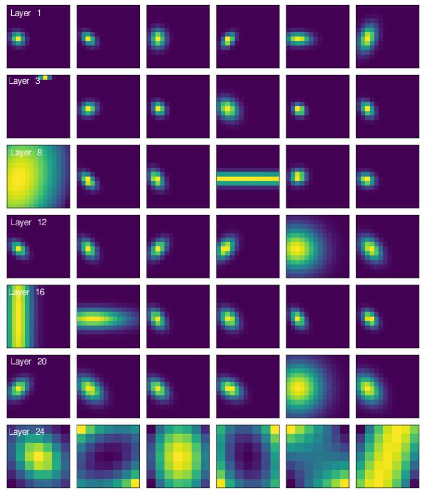
(c) $\mathbf{\Sigma}=\mathbf{\Gamma}$

Figure 4. Visualization of attention logits for a given query token with different form of covariance matrix $\mathbf{\Sigma}$. Row represents different layers and column represents the selected groups in GGQPE. Results is based on PosMLP-T

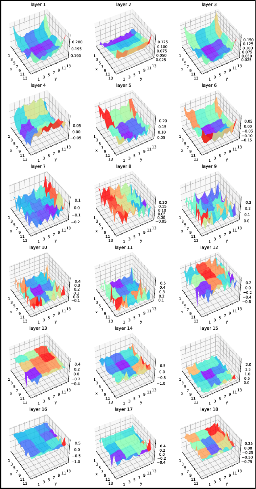
(a) gMLP/SGU

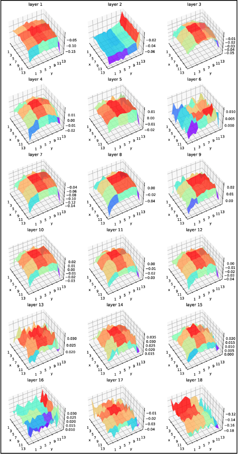
(b) PosMLP/PoSGU

Figure 5. Visualization of logits map of $\sqrt{N}\times\sqrt{N}$ bias map. (a) comes from first 18 Token FC layers (blocks) pretrained from gMLP-S and (b) uses the 18 layers of 3$th$ stages in our pretrained PosMLP-T.

5.5. Object Detection

Dataset and setting. We further examine our model on object detection using COCO2017 dataset (Lin et al., 2014). COCO2017 has 118k training images and 5k validation images. The implementation is based on the mmdetection (Chen et al., 2019) package, where two classic object detection frameworks, i.e. RetinaNet (Lin et al., 2017) and Mask R-CNN (He et al., 2017), are used. Here, the training and validation settings follow the basic protocol of Mask R-CNN and RetinaNet: 1$\times$ training scheduler (i.e., 12 epochs), batch-size 2 per GPU, resizing an image to the shorter side 800 and the longer side at most 1333, AdamW (Loshchilov and Hutter, 2017) optimizer with the initial learning rate of $1\times 10^{-4}$ and weight decay of $0.067$.

Implementation. We adopts windows shifting operation in PosMLP-T following Swin Transformer (Liu et al., 2021b) since for the large resolution dataset the non-overlap window partition will cause performance degeneration. Generally, the windows shifting operation can smooth partitioning traces and enhance windows interactions demonstrated by Swin Transformer.

Results. Table 8 shows the object detection results as well as the performance comparison with PVT (Wang et al., 2021), ResNet (He et al., 2016) and CycleMLP (Chen et al., 2022) that have similar computational complexity with our PosMLP. All PosMLP variants achieve consistent better performances than the standard convolutional networks. Secondly, PosMLP outperforms Transformer-based PVT-small on most metrics and obtain comparable results to CycleMLP but requires less parameters (e.g., 40.5M vs 46.5M, 31.1M vs 36.5M).

6. Conclusion

In this work, we have presented a new gating unit PoSGU and used it as the key building block to develop a new vision MLP architecture referred to as the PosMLP. It has the advantage of reduced parameter complexity but without sacrificed model expressive power. We have adopted two RPE mechanisms and proposed the group-wise extension to boost their performance, and these improve the weak locality and single granular non-locality in the original vision MLP design. We have conducted thorough experiments to evaluate the proposed approach, where the PosMLP exhibits high parameter and sample efficiency, e.g., Table 1 and Figure 1 (f). In the current version, we have demonstrated the merit of direct parameterization of cross-token relations for vision MLP. However, for an even larger scale pre-train dataset, a more flexible combination between RPE and TokenFC should be carefully designed, i.e., the trade-off between inductive bias and capability. We also hope this work will inspire further theoretical study of positional encoding in vision MLPs and could have a mature application as in vision Transformers.

7. ACKNOWLEDGEMENT

The work was supported in part by the National Key Research and Development Program of China (2020YFB1406703), and by the National Natural Science Foundation of China (U21B2026).

Appendix

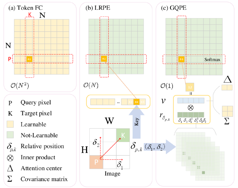
Figure 6. The demonstration of three token mixing method mentioned in this work. (a) Token FC needs to pairwisely compare the $N$ tokens; (b) The LRPE builds a learnable relation dictionary; (c) The GQPE learns the relation matrix with a constant number of parameters that is independent of $N$.

.1. Bias and APE in Object Detection

We are curious the effect of bias term and additional absolute positional encoding (APE) in the Object Detection task (under the Mash-RCNN 1x setting). This result is presented in Table 9, and it is generally consistent with the observation presented in Swim Transformer (Liu et al., 2021b), that APE is effective in image classification while it will not promote the performance in objection detection. Instead in their implementation, the extra APE will slightly degrade the performance in object detection because the APE does harm to the translation invariance . According to this phenomenon, one possible explanation is that, in comparison with the non-overlap downsample strategy adopted in Swim, we are using a convolutional downsample strategy that inherits the nature of translation invariance and will weaken the inductive bias at the end of each stage. Besides, APE is playing an important role in DETR (Carion et al., 2020) in contrast to Swim and our observation, we argue the possible explanation might be the use of multi-stage FPN and convolution-based RPN rather than the end-to-end transformer-based structure in DETR.

Table 9. Ablation study on the bias term and absolute positional encoding (APE) in objection detection.

Bias $\bm{b}$	✗	✗	✓	✓
APE	✗	✓	✗	✓
$AP^{box}$	41.6	41.6	41.6	$\mathbf{41.7}$
$AP^{mask}$	38.3	38.4	$\mathbf{38.5}$	38.4

.2. Convolutional Downsample Module

We add the ablation study at different downsampling strategy, i.e., Patch Embedding (PE) module and Patch Mearging (PM) moudle. We here demonstrates the effectiveness of using overlapping downsampling (convolutional mapping) comparing with non-overlapping downsampling (Linear mapping). Using non-overlap PM tends to introduce more redundant parameters, and substitute it with single depthwise convolution operation will siginificantly decrease both the parameter and computation complexity. The overlap PE module will slightly increase computation cost, but compared with base model it improves the accuracy of 0.75$\%$

Table 10. Performance comparison with different downsampling strategy for gMLP (with SGU).

Architecture	PE	PM	#Param.	Flops	Top-1 acc.
Original	None	None	19.4M	4.42G	72.18
Hierarchical	Linear	Linear	23.3M	5.10G	74.68
	Conv	Linear	23.3M	5.27G	75.43
	Linear	Conv	21.8M	4.93G	75.81
	Conv	Conv	21.8M	5.10G	$\mathbf{76.33}^{*}$

(a) Layer1

(b) Layer9

(c) Layer17

(d) Layer21

Figure 7. Visualization of mapping weights after training in Eq. (10.) Within each subfigure we visualize each component of projection weight matrics of different layers. In each subgraph ,the upper-left is the Token FC’s; the upper-right is the LRPE’s; The down-left is the TokenFC + LRPE’s; The down-right shows the cut line of the row index 40 in each three mapping matrics. The LRPE matrics generally have more regular patterns and keep playing a dominant term in early layers.

	Ouput size	PosMLP-T	PosMLP-S	PosMLP-B
stage 1	$C\times(56\times 56)$	$\begin{bmatrix}\text{sz.}16\times(14\times 14)\\ \text{dim}96,s8,\gamma 4,\end{bmatrix}\times 2$	$\begin{bmatrix}\text{sz.}16\times(14\times 14)\\ \text{dim}128,s8,\gamma 4,\end{bmatrix}\times 2$	$\begin{bmatrix}\text{sz.}16\times(14\times 14)\\ \text{dim}192,s8,\gamma 4,\end{bmatrix}\times 2$
stage 2	$2C\times(28\times 28)$	$\begin{bmatrix}\text{sz.}4\times(14\times 14)\\ \text{dim}192,s16,\gamma 4,\end{bmatrix}\times 2$	$\begin{bmatrix}\text{sz.}4\times(14\times 14)\\ \text{dim}256,s16,\gamma 4,\end{bmatrix}\times 2$	$\begin{bmatrix}\text{sz.}4\times(14\times 14)\\ \text{dim}384,s16,\gamma 4,\end{bmatrix}\times 2$
stage 3	$4C\times(14\times 14)$	$\begin{bmatrix}\text{sz.}1\times(14\times 14)\\ \text{dim}384,s32,\gamma 4,\end{bmatrix}\times 18$	$\begin{bmatrix}\text{sz.}1\times(14\times 14)\\ \text{dim}512,s32,\gamma 4,\end{bmatrix}\times 18$	$\begin{bmatrix}\text{sz.}1\times(14\times 14)\\ \text{dim}768,s32,\gamma 4,\end{bmatrix}\times 18$
stage 4	$8C\times(7\times 7)$	$\begin{bmatrix}\text{sz.}1\times(7\times 7)\\ \text{dim}768,s64,\gamma 2,\end{bmatrix}\times 2$	$\begin{bmatrix}\text{sz.}1\times(7\times 7)\\ \text{dim}1024,s64,\gamma 2,\end{bmatrix}\times 2$	$\begin{bmatrix}\text{sz.}1\times(7\times 7)\\ \text{dim}1536,s64,\gamma 2,\end{bmatrix}\times 2$

Table 11. Detailed architecture specifications of PosMLP.

.3. Non-Localilty

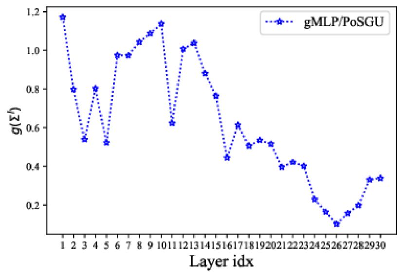
(a) gMLP/PoSGU

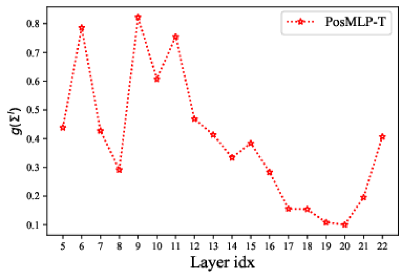
(b) PosMLP/PoSGU

Figure 8. Degree of non-local property in each PoSGU layer. The non-locality is measured by the designed matrix $g(\tilde{\Sigma}^{l})$ where $\mathbf{\Sigma}$ is the covariance matrix. The smaller of $g(\tilde{\Sigma}^{l})$ indicates this layer tends to capture more non-local patterns.

Since a $\mathbf{\Sigma}$ determines the logits distribution, it can reveal the non-locality property of the model. Typically the smaller eigenvalues of $\mathbf{\Sigma}$ will help query token attend more to other tokens. Thus we define a matrix to quantitatively visualize the non-localilty as follow:

(16) $$g(\mathbf{\Sigma}^{l})=\frac{1}{s}\sum\limits_{i=1}^{s}\sqrt{\prod\limits_{j=1}^{2}\mathbf{\lambda}^{l}_{i,j}}.$$

Where, $\lambda$ is the eigenvalue of $\mathbf{\Sigma}$ and $l$ indicates the layer index. As discussed by Cordonnier et al (Cordonnier et al., 2019), some $\mathbf{\Sigma}$ tend to be singular or close to $\mathbf{0}$, i.e., some $\lambda$ are extremely small. We do not take those $\mathbf{\Sigma}$ into account and visualize the results of gMLP/PoSGU and PoSMLP ($3th$ stage) in Figure 8. The deeper layer tends to have smaller $g(\mathbf{\Sigma}^{l})$ which indicates the stronger capability of modeling non-locality. Though the deepest layers slightly become more local, it is consistent with the observation in ConViT (d’Ascoli et al., 2021) that the localilty is not monotonically decreasing.

.4. Model Complexity Analysis

In this part, we give the parameter and computational complexities of the PosMLP block (Single window) and gMLP block. For notation clarity, we denote: input tensor map size as $(H,W,d)$; token number $N=H\times W$; channel expansion ratio in PosMLP block as $\gamma$; group number is denoted as $s$. As such, the parameters number of FC layers in the PosMLP block and gMLP block can be calculated as follows:

$$P(gMLP) =\frac{3}{2}\gamma d^{2}+(\gamma+1)d+N^{2}+N,$$

$$P(PosMLP/GLRPE) =\frac{3}{2}\gamma d^{2}+(\gamma+1)d+(4s+1)N-4s\sqrt{N}+4s,$$

$$P(PosMLP/GGRPE) =\frac{3}{2}\gamma d^{2}+(\gamma+1)d+N+6s.$$

The parameters modeling token-mixing significantly shrinks (i.e., $N^{2}\rightarrow 6s$). Their computational complexities are:

$$\Omega(gMLP) =\frac{3}{2}\gamma d^{2}N+\frac{1}{2}\gamma dN^{2},$$

$$\Omega(PosMLP/GLRPE) =\frac{3}{2}\gamma d^{2}N+\frac{1}{2}\gamma dN^{2}+sN^{2},$$

$$\Omega(PosMLP/GGRPE) =\frac{3}{2}\gamma d^{2}N+\frac{1}{2}\gamma dN^{2}+5sN^{2}.$$

Compared with the first two terms, the extra term $5sN^{2}$ is typically small and bearable.

References

- (1)
- Ba et al. (2016) Jimmy Lei Ba, Jamie Ryan Kiros, and Geoffrey E Hinton. 2016. Layer normalization. arXiv preprint arXiv:1607.06450 (2016).
- Bhojanapalli et al. (2021) Srinadh Bhojanapalli, Ayan Chakrabarti, Daniel Glasner, Daliang Li, Thomas Unterthiner, and Andreas Veit. 2021. Understanding robustness of transformers for image classification. In Proceedings of the IEEE/CVF International Conference on Computer Vision. 10231–10241.
- Carion et al. (2020) Nicolas Carion, Francisco Massa, Gabriel Synnaeve, Nicolas Usunier, Alexander Kirillov, and Sergey Zagoruyko. 2020. End-to-end object detection with transformers. In European Conference on Computer Vision. Springer, 213–229.
- Chen et al. (2019) Kai Chen, Jiaqi Wang, Jiangmiao Pang, Yuhang Cao, Yu Xiong, Xiaoxiao Li, Shuyang Sun, Wansen Feng, Ziwei Liu, Jiarui Xu, et al. 2019. MMDetection: Open mmlab detection toolbox and benchmark. arXiv preprint arXiv:1906.07155 (2019).
- Chen et al. (2022) Shoufa Chen, Enze Xie, Chongjian GE, Runjian Chen, Ding Liang, and Ping Luo. 2022. CycleMLP: A MLP-like Architecture for Dense Prediction. In International Conference on Learning Representations. https://openreview.net/forum?id=NMEceG4v69Y
- Cheng et al. (2018) Lechao Cheng, Chengyi Zhang, and Zicheng Liao. 2018. Intrinsic image transformation via scale space decomposition. In Proceedings of the IEEE conference on computer vision and pattern recognition. 656–665.
- Chu et al. (2021) Xiangxiang Chu, Zhi Tian, Bo Zhang, Xinlong Wang, Xiaolin Wei, Huaxia Xia, and Chunhua Shen. 2021. Conditional positional encodings for vision transformers. arXiv preprint arXiv:2102.10882 (2021).
- Cordonnier et al. (2019) Jean-Baptiste Cordonnier, Andreas Loukas, and Martin Jaggi. 2019. On the relationship between self-attention and convolutional layers. arXiv preprint arXiv:1911.03584 (2019).
- Cubuk et al. (2020) Ekin D Cubuk, Barret Zoph, Jonathon Shlens, and Quoc V Le. 2020. Randaugment: Practical automated data augmentation with a reduced search space. In Proceedings of the IEEE/CVF Conference on Computer Vision and Pattern Recognition Workshops. 702–703.
- Dai et al. (2021) Zihang Dai, Hanxiao Liu, Quoc Le, and Mingxing Tan. 2021. Coatnet: Marrying convolution and attention for all data sizes. Advances in Neural Information Processing Systems 34 (2021).
- Deng et al. (2009) Jia Deng, Wei Dong, Richard Socher, Li-Jia Li, Kai Li, and Li Fei-Fei. 2009. Imagenet: A large-scale hierarchical image database. In 2009 IEEE conference on computer vision and pattern recognition. Ieee, 248–255.
- Ding et al. (2021) Xiaohan Ding, Xiangyu Zhang, Jungong Han, and Guiguang Ding. 2021. RepMLP: Re-parameterizing Convolutions into Fully-connected Layers for Image Recognition. arXiv preprint arXiv:2105.01883 (2021).
- Dong et al. (2021) Xiaoyi Dong, Jianmin Bao, Dongdong Chen, Weiming Zhang, Nenghai Yu, Lu Yuan, Dong Chen, and Baining Guo. 2021. Cswin transformer: A general vision transformer backbone with cross-shaped windows. arXiv preprint arXiv:2107.00652 (2021).
- Dosovitskiy et al. (2021) Alexey Dosovitskiy, Lucas Beyer, Alexander Kolesnikov, Dirk Weissenborn, Xiaohua Zhai, Thomas Unterthiner, Mostafa Dehghani, Matthias Minderer, Georg Heigold, Sylvain Gelly, Jakob Uszkoreit, and Neil Houlsby. 2021. An Image is Worth 16x16 Words: Transformers for Image Recognition at Scale. In International Conference on Learning Representations. https://openreview.net/forum?id=YicbFdNTTy
- d’Ascoli et al. (2021) Stéphane d’Ascoli, Hugo Touvron, Matthew L Leavitt, Ari S Morcos, Giulio Biroli, and Levent Sagun. 2021. Convit: Improving vision transformers with soft convolutional inductive biases. In International Conference on Machine Learning. PMLR, 2286–2296.
- Fang et al. (2022) Chaowei Fang, Dingwen Zhang, Liang Wang, Yulun Zhang, Lechao Cheng, and Junwei Han. 2022. Cross-Modality High-Frequency Transformer for MR Image Super-Resolution. arXiv preprint arXiv:2203.15314 (2022).
- Guo et al. (2021) Jianyuan Guo, Yehui Tang, Kai Han, Xinghao Chen, Han Wu, Chao Xu, Chang Xu, and Yunhe Wang. 2021. Hire-MLP: Vision MLP via Hierarchical Rearrangement. arXiv preprint arXiv:2108.13341 (2021).
- Hao et al. (2022) Yanbin Hao, Hao Zhang, Chong-Wah Ngo, and Xiangnan He. 2022. Group Contextualization for Video Recognition. In Proceedings of the IEEE/CVF Conference on Computer Vision and Pattern Recognition. 928–938.
- He et al. (2017) Kaiming He, Georgia Gkioxari, Piotr Dollár, and Ross Girshick. 2017. Mask r-cnn. In Proceedings of the IEEE international conference on computer vision. 2961–2969.
- He et al. (2016) Kaiming He, Xiangyu Zhang, Shaoqing Ren, and Jian Sun. 2016. Deep residual learning for image recognition. In Proceedings of the IEEE conference on computer vision and pattern recognition. 770–778.
- He et al. (2020) Pengcheng He, Xiaodong Liu, Jianfeng Gao, and Weizhu Chen. 2020. Deberta: Decoding-enhanced bert with disentangled attention. arXiv preprint arXiv:2006.03654 (2020).
- Hinton et al. (2015) Geoffrey Hinton, Oriol Vinyals, and Jeff Dean. 2015. Distilling the knowledge in a neural network. arXiv preprint arXiv:1503.02531 (2015).
- Hou et al. (2022) Qibin Hou, Zihang Jiang, Li Yuan, Ming-Ming Cheng, Shuicheng Yan, and Jiashi Feng. 2022. Vision permutator: A permutable mlp-like architecture for visual recognition. IEEE Transactions on Pattern Analysis and Machine Intelligence (2022).
- Hu et al. (2018) Han Hu, Jiayuan Gu, Zheng Zhang, Jifeng Dai, and Yichen Wei. 2018. Relation networks for object detection. In Proceedings of the IEEE conference on computer vision and pattern recognition. 3588–3597.
- Hu et al. (2019) Han Hu, Zheng Zhang, Zhenda Xie, and Stephen Lin. 2019. Local relation networks for image recognition. In Proceedings of the IEEE/CVF International Conference on Computer Vision. 3464–3473.
- Huang et al. (2016) Gao Huang, Yu Sun, Zhuang Liu, Daniel Sedra, and Kilian Q Weinberger. 2016. Deep networks with stochastic depth. In European conference on computer vision. Springer, 646–661.
- Huang et al. (2020) Zhiheng Huang, Davis Liang, Peng Xu, and Bing Xiang. 2020. Improve transformer models with better relative position embeddings. arXiv preprint arXiv:2009.13658 (2020).
- Ju et al. (2020) Xincheng Ju, Dong Zhang, Junhui Li, and Guodong Zhou. 2020. Transformer-based label set generation for multi-modal multi-label emotion detection. In Proceedings of the 28th ACM International Conference on Multimedia. 512–520.
- Ke et al. (2020) Guolin Ke, Di He, and Tie-Yan Liu. 2020. Rethinking positional encoding in language pre-training. arXiv preprint arXiv:2006.15595 (2020).
- Krizhevsky et al. (2012) Alex Krizhevsky, Ilya Sutskever, and Geoffrey E Hinton. 2012. Imagenet classification with deep convolutional neural networks. Advances in neural information processing systems 25 (2012), 1097–1105.
- Lian et al. (2021) Dongze Lian, Zehao Yu, Xing Sun, and Shenghua Gao. 2021. As-mlp: An axial shifted mlp architecture for vision. arXiv preprint arXiv:2107.08391 (2021).
- Likhomanenko et al. (2021) Tatiana Likhomanenko, Qiantong Xu, Gabriel Synnaeve, Ronan Collobert, and Alex Rogozhnikov. 2021. CAPE: Encoding relative positions with continuous augmented positional embeddings. Advances in Neural Information Processing Systems 34 (2021), 16079–16092.
- Lin et al. (2017) Tsung-Yi Lin, Priya Goyal, Ross Girshick, Kaiming He, and Piotr Dollár. 2017. Focal loss for dense object detection. In Proceedings of the IEEE international conference on computer vision. 2980–2988.
- Lin et al. (2014) Tsung-Yi Lin, Michael Maire, Serge Belongie, James Hays, Pietro Perona, Deva Ramanan, Piotr Dollár, and C Lawrence Zitnick. 2014. Microsoft coco: Common objects in context. In European conference on computer vision. Springer, 740–755.
- Liu et al. (2021a) Hanxiao Liu, Zihang Dai, David So, and Quoc Le. 2021a. Pay attention to MLPs. Advances in Neural Information Processing Systems 34 (2021).
- Liu et al. (2021b) Ze Liu, Yutong Lin, Yue Cao, Han Hu, Yixuan Wei, Zheng Zhang, Stephen Lin, and Baining Guo. 2021b. Swin transformer: Hierarchical vision transformer using shifted windows. In Proceedings of the IEEE/CVF International Conference on Computer Vision. 10012–10022.
- Loshchilov and Hutter (2017) Ilya Loshchilov and Frank Hutter. 2017. Decoupled weight decay regularization. arXiv preprint arXiv:1711.05101 (2017).
- Polyak and Juditsky (1992) Boris T Polyak and Anatoli B Juditsky. 1992. Acceleration of stochastic approximation by averaging. SIAM journal on control and optimization 30, 4 (1992), 838–855.
- Radford et al. (2018) Alec Radford, Karthik Narasimhan, Tim Salimans, and Ilya Sutskever. 2018. Improving language understanding by generative pre-training. (2018).
- Radford et al. (2019) Alec Radford, Jeffrey Wu, Rewon Child, David Luan, Dario Amodei, Ilya Sutskever, et al. 2019. Language models are unsupervised multitask learners. OpenAI blog 1, 8 (2019), 9.
- Radosavovic et al. (2020) Ilija Radosavovic, Raj Prateek Kosaraju, Ross Girshick, Kaiming He, and Piotr Dollár. 2020. Designing network design spaces. In Proceedings of the IEEE/CVF Conference on Computer Vision and Pattern Recognition. 10428–10436.
- Raffel et al. (2019) Colin Raffel, Noam Shazeer, Adam Roberts, Katherine Lee, Sharan Narang, Michael Matena, Yanqi Zhou, Wei Li, and Peter J Liu. 2019. Exploring the limits of transfer learning with a unified text-to-text transformer. arXiv preprint arXiv:1910.10683 (2019).
- Shaw et al. (2018) Peter Shaw, Jakob Uszkoreit, and Ashish Vaswani. 2018. Self-attention with relative position representations. arXiv preprint arXiv:1803.02155 (2018).
- Simoncelli and Olshausen (2001) Eero P Simoncelli and Bruno A Olshausen. 2001. Natural image statistics and neural representation. Annual review of neuroscience 24, 1 (2001), 1193–1216.
- Tolstikhin et al. (2021) Ilya O Tolstikhin, Neil Houlsby, Alexander Kolesnikov, Lucas Beyer, Xiaohua Zhai, Thomas Unterthiner, Jessica Yung, Andreas Steiner, Daniel Keysers, Jakob Uszkoreit, et al. 2021. Mlp-mixer: An all-mlp architecture for vision. Advances in Neural Information Processing Systems 34 (2021).
- Touvron et al. (2021a) Hugo Touvron, Piotr Bojanowski, Mathilde Caron, Matthieu Cord, Alaaeldin El-Nouby, Edouard Grave, Gautier Izacard, Armand Joulin, Gabriel Synnaeve, Jakob Verbeek, et al. 2021a. Resmlp: Feedforward networks for image classification with data-efficient training. arXiv preprint arXiv:2105.03404 (2021).
- Touvron et al. (2021b) Hugo Touvron, Matthieu Cord, Matthijs Douze, Francisco Massa, Alexandre Sablayrolles, and Hervé Jégou. 2021b. Training data-efficient image transformers & distillation through attention. In International Conference on Machine Learning. PMLR, 10347–10357.
- Vaswani et al. (2017) Ashish Vaswani, Noam Shazeer, Niki Parmar, Jakob Uszkoreit, Llion Jones, Aidan N Gomez, Łukasz Kaiser, and Illia Polosukhin. 2017. Attention is all you need. In Advances in neural information processing systems. 5998–6008.
- Wang et al. (2021) Wenhai Wang, Enze Xie, Xiang Li, Deng-Ping Fan, Kaitao Song, Ding Liang, Tong Lu, Ping Luo, and Ling Shao. 2021. Pyramid vision transformer: A versatile backbone for dense prediction without convolutions. In Proceedings of the IEEE/CVF International Conference on Computer Vision. 568–578.
- Wu et al. (2021) Kan Wu, Houwen Peng, Minghao Chen, Jianlong Fu, and Hongyang Chao. 2021. Rethinking and improving relative position encoding for vision transformer. In Proceedings of the IEEE/CVF International Conference on Computer Vision. 10033–10041.
- Xiao et al. (2021) Tete Xiao, Mannat Singh, Eric Mintun, Trevor Darrell, Piotr Dollár, and Ross Girshick. 2021. Early convolutions help transformers see better. arXiv preprint arXiv:2106.14881 (2021).
- Yu et al. (2022) Tan Yu, Xu Li, Yunfeng Cai, Mingming Sun, and Ping Li. 2022. S2-mlp: Spatial-shift mlp architecture for vision. In Proceedings of the IEEE/CVF Winter Conference on Applications of Computer Vision. 297–306.
- Yun et al. (2019) Sangdoo Yun, Dongyoon Han, Seong Joon Oh, Sanghyuk Chun, Junsuk Choe, and Youngjoon Yoo. 2019. Cutmix: Regularization strategy to train strong classifiers with localizable features. In Proceedings of the IEEE/CVF International Conference on Computer Vision. 6023–6032.
- Zhang et al. (2017) Hongyi Zhang, Moustapha Cisse, Yann N Dauphin, and David Lopez-Paz. 2017. mixup: Beyond empirical risk minimization. arXiv preprint arXiv:1710.09412 (2017).
- Zhang et al. (2021a) Hao Zhang, Yanbin Hao, and Chong-Wah Ngo. 2021a. Token shift transformer for video classification. In Proceedings of the 29th ACM International Conference on Multimedia. 917–925.
- Zhang et al. (2021b) Zizhao Zhang, Han Zhang, Long Zhao, Ting Chen, and Tomas Pfister. 2021b. Aggregating nested transformers. arXiv preprint arXiv:2105.12723 (2021).
- Zhong et al. (2020) Zhun Zhong, Liang Zheng, Guoliang Kang, Shaozi Li, and Yi Yang. 2020. Random erasing data augmentation. In Proceedings of the AAAI Conference on Artificial Intelligence, Vol. 34. 13001–13008.