Steer: Beam Selection for Full-Duplex
Millimeter Wave Communication Systems

Abstract

Modern millimeter wave (mmWave) communication systems rely on beam alignment to deliver sufficient beamforming gain to close the link between devices. We present a novel beam selection methodology for multi-panel, full-duplex mmWave systems, which we call Steer, that delivers high beamforming gain while significantly reducing the full-duplex self-interference coupled between the transmit and receive beams. Steer does not necessitate changes to conventional beam alignment methodologies nor additional over-the-air feedback, making it compatible with existing cellular standards. Instead, Steer uses conventional beam alignment to identify the general directions beams should be steered, and then it makes use of a minimal number of self-interference measurements to jointly select transmit and receive beams that deliver high gain in these directions while coupling low self-interference. We implement Steer on an industry-grade 28 GHz phased array platform and use further simulation to show that full-duplex operation with beams selected by Steer can notably outperform both half-duplex and full-duplex operation with beams chosen via conventional beam selection. For instance, Steer can reliably reduce self-interference by more than $20$ dB and improve SINR by more than $10$ dB, compared to conventional beam selection. Our experimental results highlight that beam alignment can be used not only to deliver high beamforming gain in full-duplex mmWave systems but also to mitigate self-interference to levels near or below the noise floor, rendering additional self-interference cancellation unnecessary with Steer.

I Introduction

To equip millimeter wave (mmWave) transceivers with full-duplex capability, recent work has proposed leveraging dense antenna arrays to mitigate self-interference spatially via strategic beamforming [1, 2, 3, 4, 5, 6, 7, 8, 9, 10, 11, 12, 13, 14, 15, 16, 17]. For instance, in [9, 10, 11, 16, 15, 12, 13, 14], designs are presented that tailor hybrid beamformers at a mmWave transceiver to mitigate self-interference while maintaining transmission and reception. Proposed solutions [17, 18, 19, 20, 21, 22, 23] have also suggested using analog and digital self-interference cancellation to enable mmWave full-duplex; solutions like these require additional hardware, demand complex digital signal processing, and/or do not scale well to systems with many antennas. For these reasons, the scope of the present paper focuses on using beamforming alone to mitigate self-interference spatially, which does not require dedicated hardware nor complex signal processing. If successfully equipped with full-duplex capability, mmWave communication systems could see impressive throughput and latency enhancements, which magnify at the network level and facilitate integrated access and backhaul (IAB) deployments [24].

Most proposed beamforming-based solutions to mitigate self-interference are not well-suited for practical systems for a few reasons. First, many practical mmWave systems are equipped with analog beamforming but lack digital beamforming, rendering proposed hybrid beamforming designs (e.g., [9, 10, 11, 16, 15, 12, 13, 14]) unfit for such systems. This is especially problematic since digital beamforming mitigates the large majority of self-interference in most of these designs. Proposed designs [6, 5, 7, 8] that rely solely on analog beamforming (rather than hybrid beamforming) are also impractical for a few reasons. These rely on instantaneous knowledge of the self-interference channel—a high-dimensional multiple-input multiple-output (MIMO) channel—whose real-time estimation is currently impractical due to complications posed by analog beamforming and its sheer size. Furthermore, [6, 10, 7, 8, 9, 15, 11, 12, 13, 14] require instantaneous knowledge of the downlink and uplink MIMO channels between a full-duplex transceiver and the devices it serves; even this is currently impractical in mmWave networks, which circumvent MIMO channel estimation via beam alignment. Some designs [9, 6, 10, 8, 7, 11, 15] do not account for phase shifters and/or attenuators with limited resolution that practical analog beamforming networks are subjected to.

Many proposed beamforming designs for full-duplex mmWave systems do not accommodate beam alignment and subsequent analog beam selection [6, 10, 9, 8, 7, 11, 12, 13, 14]. Beam alignment is a critical component of practical mmWave systems to provide sufficient link margin to sustain communication without the need for uplink/downlink MIMO channel knowledge [25, 26]. Using measurements from beam alignment, a mmWave system can configure its analog beamformers through beam selection. Conventional half-duplex systems typically aim to overcome severe path loss by selecting beams that maximize received signal-to-noise ratio (SNR). Like half-duplex mmWave systems, a full-duplex one will presumably execute beam selection and will do so on its transmit link and receive link. Naively applying conventional beam selection on the two links independently, however, does not account for self-interference that couples between the transmit and receive beams when operating in a full-duplex fashion. This has motivated us to create the first beam selection methodology for full-duplex systems. The two principal contributions of this paper are summarized as follows.

A beam selection methodology for full-duplex systems. We present Steer, the first beam selection methodology for jointly selecting the transmit and receive beams of a full-duplex mmWave transceiver. To do so, we leverage our observations from a recent measurement campaign of mmWave self-interference [27, 28], which showed that small shifts in the steering directions of the transmit and receive beams (on the order of one degree) can lead to noteworthy reductions in self-interference. Steer makes use of self-interference measurements across small spatial neighborhoods to jointly select transmit and receive beams at the full-duplex device that offer reduced self-interference while delivering high beamforming gain on the uplink and downlink. Following its formulation, we present an algorithm for executing Steer with a minimal number of self-interference measurements. The execution of Steer takes place only at the full-duplex device, introducing no changes to the devices being served nor additional over-the-air feedback, making it compatible with existing beam alignment schemes.

Validation of Steer through measurement and simulation. We validate Steer by combining simulation with self-interference measurements from an industry-grade 28 GHz phased array platform. These experimental results illustrate that full-duplex operation with Steer can offer a sum spectral efficiency notably higher than both half-duplex and full-duplex operation with beams from conventional beam alignment. In fact, in most cases, Steer can reduce self-interference to levels such that no additional cancellation is warranted (i.e., near or below the noise floor). With Steer, beamforming alone can deliver self-interference mitigation sufficient for full-duplex while importantly accommodating beam alignment, even in the presence of cross-link interference arising when serving devices simultaneously and in-band.

II System Model

As a relevant application of this work, we consider the mmWave communication system shown in Figure 1, where a sectorized, multi-panel IAB node maintains backhaul and serves access in a full-duplex fashion (i.e., on the same time-frequency resources) [29]. This is particularly attractive application of full-duplex in mmWave cellular systems [30, 31], but the contributions of this work are not limited to IAB. Illustrated in Figure 1 is the downlink-downlink (DL-DL) operating mode, where an IAB node receives backhaul from a fiber-connected donor and transmits access to a user equipment (UE). In this work, we present a formulation and design that generalizes to both the DL-DL operating mode and the analogous uplink-uplink (UL-UL) mode where the IAB node receives access and transmits backhaul. We are particularly interested in these full-duplex operating modes since they unlock scheduling opportunities that can reduce latency in IAB networks while also increasing throughput [24]. It is important to consider and evaluate both full-duplexing modes since there may exist significant disparities between the donor and UE—most notably transmit power, noise power, and number of antennas.

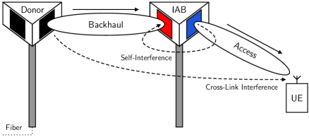
Figure 1: A full-duplex IAB node receives backhaul from a fiber-connected donor node while simultaneously transmitting access to a UE, giving rise to self-interference at the IAB node and cross-link interference at the UE. We refer to this as the DL-DL operating mode. We also consider the UL-UL mode where the UE transmits uplink access and the IAB node transmits backhaul.

Separate uniform planar arrays (UPAs) are present at the IAB node, each of which can either transmit or receive and can be independently configured via a network of analog beamforming weights. In this multi-panel full-duplex setting, one array will transmit while the other receives. To simplify notation between the DL-DL and UL-UL modes, we assume each array at the IAB node is equipped with $N_{\mathrm{a}}$ antennas. We denote the vector of transmit beamforming weights at the IAB node as ${\mathbf{f}}\in\mathbb{C}^{N_{\mathrm{a}}\times 1}$. Likewise, the receive beamforming vector at the IAB node is denoted ${\mathbf{w}}\in\mathbb{C}^{N_{\mathrm{a}}\times 1}$. For transmit power and noise power normalizations, we assume that the beamforming weights have unit power as ${\left\|{\mathbf{f}}\right\|}_{2}^{2}={\left\|{\mathbf{w}}\right\|}_{2}^{2}=1$. Extending this work to systems with multiple beams at the transmitter and receiver would be great future work.

For simplicity, we assume the UE is a single-antenna device, though the work herein could extend naturally to those with multiple antennas. Let the row vector ${\mathbf{h}}_{\mathrm{AC}}^{{*}}\in\mathbb{C}^{1\times N_{\mathrm{a}}}$ be the access channel between the transmit array of the IAB node and the UE. Practically, the donor will have an antenna array through which it serves backhaul. With an array at the donor and an array at the IAB node, we use ${\mathbf{H}}_{\mathrm{BH}}$ to denote the MIMO backhaul channel matrix between the donor and the receive panel of the IAB node. We assume the donor transmits with some beamforming weights ${\mathbf{v}}$ and instead consider henceforth the column vector

$${\mathbf{h}}_{\mathrm{BH}}\triangleq{\mathbf{H}}_{\mathrm{BH}}{\mathbf{v}}\in\mathbb{C}^{N_{\mathrm{a}}\times 1}$$ (1)

which is the effective backhaul channel from the beamformed donor to the IAB node—abstracting out beamforming at the donor. We normalize the access and backhaul channel vectors as ${\left\|{\mathbf{h}}_{\mathrm{AC}}\right\|}_{2}^{2}={\left\|{\mathbf{h}}_{\mathrm{BH}}\right\|}_{2}^{2}=N_{\mathrm{a}}$ and abstract out their large-scale path gains (inverse path loss) as $G_{\mathrm{AC}}^{2}$ and $G_{\mathrm{BH}}^{2}$, respectively. We invite readers to assume access and backhaul channels that are line-of-sight (LOS) for simplicity, but this work does not depend on such.

In the DL-DL operating mode—when transmitting access and receiving backhaul from the IAB node in a full-duplex fashion—a MIMO self-interference channel ${\mathbf{H}}_{\mathrm{SI}}\in\mathbb{C}^{N_{\mathrm{a}}\times N_{\mathrm{a}}}$ manifests between the transmit and receive arrays of the IAB node. We similarly abstract out its large-scale path gain as $G_{\mathrm{SI}}^{2}$ and enforce ${\left\|{\mathbf{H}}_{\mathrm{SI}}\right\|}_{\mathrm{F}}^{2}=N_{\mathrm{a}}^{2}$. In addition, during DL-DL, since the donor transmits backhaul while the UE receives access, a cross-link interference channel ${\mathbf{h}}_{\mathrm{CL}}^{{*}}$ (a row vector) manifests between the donor’s antenna array and the UE. Having conditioned on some beamforming weights ${\mathbf{v}}$ at the donor, the effective cross-link interference channel is the scalar

$$h_{\mathrm{CL}}\triangleq{\mathbf{h}}_{\mathrm{CL}}^{{*}}{\mathbf{v}}\in\mathbb{C}^{1\times 1}.$$ (2)

We similarly abstract out its large-scale gain as $G_{\mathrm{CL}}^{2}$ by letting ${\left|h_{\mathrm{CL}}\right|}^{2}=1$. Symbols are transmitted by the donor, IAB node, and UE with powers (in watts) $P_{\mathrm{tx}}^{\mathrm{Don}}$, $P_{\mathrm{tx}}^{\mathrm{IAB}}$, and $P_{\mathrm{tx}}^{\mathrm{UE}}$, respectively. Additive noise incurred at the donor, IAB node, and UE have respective powers (in watts) $P_{\mathrm{noise}}^{\mathrm{Don}}$, $P_{\mathrm{noise}}^{\mathrm{IAB}}$, and $P_{\mathrm{noise}}^{\mathrm{UE}}$. With these definitions in hand, we can formulate the quality of each link in the DL-DL and UL-UL modes.

III Problem Formulation and Motivation

TABLE I: The transmit and receive links during different full-duplexing modes.

Mode	Transmit Link	Receive Link
Downlink-Downlink	Access	Backhaul
Uplink-Uplink	Backhaul	Access

We leverage our formulations of the DL-DL and UL-UL modes to present a general formulation of the system. Taking the perspective of the full-duplex IAB node, we introduce the terms transmit link and receive link, which correspond to either access or backhaul depending on if the system operates in DL-DL or UL-UL mode, as summarized in Table I. In the DL-DL mode, for instance, the SNR of the transmit link and receive link can be expressed respectively as

$$\mathsf{SNR}_{\mathrm{tx}} =\frac{P_{\mathrm{tx}}^{\mathrm{IAB}}\cdot G_{\mathrm{AC}}^{2}\cdot{\left|{\mathbf{h}}_{\mathrm{AC}}^{{*}}{\mathbf{f}}\right|}^{2}}{P_{\mathrm{noise}}^{\mathrm{UE}}},\qquad\mathsf{SNR}_{\mathrm{rx}}=\frac{P_{\mathrm{tx}}^{\mathrm{Don}}\cdot G_{\mathrm{BH}}^{2}\cdot{\left|{\mathbf{w}}^{{*}}{\mathbf{h}}_{\mathrm{BH}}\right|}^{2}}{P_{\mathrm{noise}}^{\mathrm{IAB}}}.$$ (3)

By virtue of the fact that $N_{\mathrm{a}}=\max_{{\mathbf{x}}}\ {\left|{\mathbf{h}}^{{*}}{\mathbf{x}}\right|}^{2}\ \mathrm{s.t.~{}}{\left\|{\mathbf{x}}\right\|}_{2}^{2}=1,{\left\|{\mathbf{h}}\right\|}_{2}^{2}=N_{\mathrm{a}}$, the maximum SNRs during the DL-DL mode, which we denote with an overline, are

$$\overline{\mathsf{SNR}}_{\mathrm{tx}}=\frac{P_{\mathrm{tx}}^{\mathrm{IAB}}\cdot G_{\mathrm{AC}}^{2}\cdot N_{\mathrm{a}}}{P_{\mathrm{noise}}^{\mathrm{UE}}}\geq\mathsf{SNR}_{\mathrm{tx}},\qquad\overline{\mathsf{SNR}}_{\mathrm{rx}}=\frac{P_{\mathrm{tx}}^{\mathrm{Don}}\cdot G_{\mathrm{BH}}^{2}\cdot N_{\mathrm{a}}}{P_{\mathrm{noise}}^{\mathrm{IAB}}}\geq\mathsf{SNR}_{\mathrm{rx}}.$$ (4)

These are achieved by beamforming directly toward the UE and donor to deliver maximum gain. In the DL-DL mode, access is corrupted by cross-link interference and backhaul is corrupted by self-interference, leading to the interference-to-noise ratio (INR) of the transmit and receive links being respectively

$$\mathsf{INR}_{\mathrm{tx}} =\frac{P_{\mathrm{tx}}^{\mathrm{Don}}\cdot G_{\mathrm{CL}}^{2}\cdot{\left|h_{\mathrm{CL}}\right|}^{2}}{P_{\mathrm{noise}}^{\mathrm{UE}}},\qquad\mathsf{INR}_{\mathrm{rx}}=\frac{P_{\mathrm{tx}}^{\mathrm{IAB}}\cdot G_{\mathrm{SI}}^{2}\cdot{\left|{\mathbf{w}}^{{*}}{\mathbf{H}}_{\mathrm{SI}}{\mathbf{f}}\right|}^{2}}{P_{\mathrm{noise}}^{\mathrm{IAB}}}.$$ (5)

Notice that the degree of self-interference depends on its channel ${\mathbf{H}}_{\mathrm{SI}}$ and the beamformers ${\mathbf{f}}$ and ${\mathbf{w}}$ at the IAB node. Cross-link interference, on the other hand, does not depend on ${\mathbf{f}}$ nor ${\mathbf{w}}$ and is fixed for a given setting, having conditioned on the donor’s beamformer ${\mathbf{v}}$. All terms presented here for the DL-DL mode can be defined analogously for the UL-UL mode, with backhaul as the transmit link and access as the receive link. Note that, regardless of operating mode, the transmit link is plagued by cross-link interference and the receive link is plagued by self-interference.

With these formulations of the transmit and receive links, their signal-to-interference-plus-noise ratios (SINRs) can be written as

$$\mathsf{SINR}_{\mathrm{tx}}=\frac{\mathsf{SNR}_{\mathrm{tx}}}{1+\mathsf{INR}_{\mathrm{tx}}},\qquad\mathsf{SINR}_{\mathrm{rx}}=\frac{\mathsf{SNR}_{\mathrm{rx}}}{1+\mathsf{INR}_{\mathrm{rx}}}.$$ (6)

Treating interference as noise, the maximum achievable spectral efficiencies on each link are

$$R_{\mathrm{tx}} =\mathrm{log}_{2}{\left(1+\mathsf{SINR}_{\mathrm{tx}}\right)},\qquad R_{\mathrm{rx}}=\mathrm{log}_{2}{\left(1+\mathsf{SINR}_{\mathrm{rx}}\right)}$$ (7)

whereas the individual Shannon capacities of each of these links are

$$C_{\mathrm{tx}} =\mathrm{log}_{2}{\left(1+\overline{\mathsf{SNR}}_{\mathrm{tx}}\right)},\qquad C_{\mathrm{rx}}=\mathrm{log}_{2}{\left(1+\overline{\mathsf{SNR}}_{\mathrm{rx}}\right)}.$$ (8)

In this paper, we seek a means to strategically select beams ${\mathbf{f}}$ and ${\mathbf{w}}$ such that self-interference can be significantly reduced and spectral efficiency can be improved over conventional/naive approaches. Taking a full-duplex perspective, we desire a sum spectral efficiency $R_{\mathrm{tx}}+R_{\mathrm{rx}}$ that approaches the full-duplex capacity $C_{\mathrm{tx}}+C_{\mathrm{rx}}$. In this pursuit, we account for a number of practical considerations in this work, most notably limited channel knowledge and practical codebook-based beam alignment.

In this work, we aim to leverage small-scale phenomena observed in our recent measurement campaign [27, 28] by slightly shifting transmit and receive beams so that self-interference (i.e., $\mathsf{INR}_{\mathrm{rx}}$) can be reduced while still delivering high beamforming gain (i.e., high $\mathsf{SNR}_{\mathrm{tx}}$ and $\mathsf{SNR}_{\mathrm{rx}}$) in the desired directions. To do this in a systematic manner, we introduce the first beam selection methodology specifically for full-duplex mmWave systems, called Steer, that makes use of self-interference measurements to choose beams that reduce self-interference and facilitate full-duplex operation. In fact, we show that Steer can reduce self-interference to levels sufficiently low for full-duplex operation without the need for any additional analog nor digital cancellation. This is particularly desirable because it removes the need for additional hardware and signal processing that conventional self-interference cancellation strategies demand. In the sections that follow, we present the three components of Steer:

1. initial beam selection via conventional beam alignment (Section IV);

2. measurements of self-interference across small spatial neighborhoods (Section V); these are not necessarily taken in real-time but rather periodically as needed;

3. final beam selection to minimize self-interference (Section VI).

A block diagram summarizing Steer is shown in Figure 2, whose details will become clear as we present our design in the next three sections.

Figure 2: A block diagram summarizing beam selection via Steer, which jointly selects transmit and receive beams to reduce self-interference. Conventional beam selection chooses transmit and receive beams independently, ignoring self-interference.

IV Initial Beam Selection: Conventional Beam Alignment

Practical mmWave communication systems rely on beam alignment schemes to deliver high beamforming gain. These schemes typically involve sweeping candidate beams, measuring the reference signal received power (RSRP) for each candidate, and delivering feedback before determining the beam(s) for the mmWave link [25, 26]. Candidate beams often come from a codebook, which is constructed by first defining a service region (some portion of space based on an assumed user distribution) and then discretizing it based on the desired number of beams in the codebook or their beamwidth.

In a traditional half-duplex fashion, we suppose the IAB node conducts beam alignment on its transmit link with $N_{\mathrm{tx}}$ beams and on its receive link with $N_{\mathrm{rx}}$ beams. The $N_{\mathrm{tx}}$ transmit beams and $N_{\mathrm{rx}}$ receive beams are spatially distributed over their desired coverage regions, where each beam is responsible for serving some portion of its respective region. Describing the steering direction of each beam in an azimuth-elevation fashion, the collection of transmit directions $\mathcal{A}_{\mathrm{tx}}$ and receive directions $\mathcal{A}_{\mathrm{rx}}$ we write as

$$\mathcal{A}_{\mathrm{tx}} ={\left\{{\left(\theta_{\mathrm{tx}}^{{\left(i\right)}},\phi_{\mathrm{tx}}^{{\left(i\right)}}\right)}:i=1,\dots,N_{\mathrm{tx}}\right\}},\qquad\mathcal{A}_{\mathrm{rx}}={\left\{{\left(\theta_{\mathrm{rx}}^{{\left(j\right)}},\phi_{\mathrm{rx}}^{{\left(j\right)}}\right)}:j=1,\dots,N_{\mathrm{rx}}\right\}}.$$ (9)

For instance, suppose $\mathcal{A}_{\mathrm{tx}}$ and $\mathcal{A}_{\mathrm{rx}}$ are each comprised of $N_{\mathrm{tx}}=N_{\mathrm{rx}}$ directions distributed uniformly from $-60^{\circ}$ to $60^{\circ}$ in azimuth and from $-30^{\circ}$ to $30^{\circ}$ in elevation.

Practical phased array systems are often equipped with a mapping from desired steering direction to beamforming weights based on some beam design methodology. As such, let $\mathcal{F}={\left\{{\mathbf{f}}{\left(\theta,\phi\right)}:{\left(\theta,\phi\right)}\in\mathcal{A}_{\mathrm{tx}}\right\}}$ and $\mathcal{W}={\left\{{\mathbf{w}}{\left(\theta,\phi\right)}:{\left(\theta,\phi\right)}\in\mathcal{A}_{\mathrm{rx}}\right\}}$ be the transmit and receive codebooks used for conventional beam alignment, where ${\mathbf{f}}{\left(\theta,\phi\right)}$ and ${\mathbf{w}}{\left(\theta,\phi\right)}$ are transmit and receive weights designed to steer toward some ${\left(\theta,\phi\right)}$. Let ${\mathbf{h}}_{\mathrm{tx}}^{{*}}$ and ${\mathbf{h}}_{\mathrm{rx}}$ be the transmit and receive channels corresponding to the particular operating mode. Conventional beam alignment on the transmit link aims to solve (or approximately solve)

$$i^{\star}=\operatorname*{\mathrm{argmax}}_{i\in{\left\{1,\dots,N_{\mathrm{tx}}\right\}}}\ {\left|{\mathbf{h}}_{\mathrm{tx}}^{{*}}{\mathbf{f}}{\left(\theta_{\mathrm{tx}}^{{\left(i\right)}},\phi_{\mathrm{tx}}^{{\left(i\right)}}\right)}\right|}^{2}$$ (10)

to identify the transmit beam ${\mathbf{f}}{\left(\theta_{\mathrm{tx}}^{{\left(i^{\star}\right)}},\phi_{\mathrm{tx}}^{{\left(i^{\star}\right)}}\right)}\in\mathcal{F}$ that maximizes beamforming gain delivered on the transmit link. In other words, the transmit link user—either the donor or the UE depending on the mode—is approximately located in the direction ${\left(\theta_{\mathrm{tx}}^{{\left(i^{\star}\right)}},\phi_{\mathrm{tx}}^{{\left(i^{\star}\right)}}\right)}$ from the transmit panel of the IAB node. Likewise, beam alignment on the receive link aims to solve

$$j^{\star}=\operatorname*{\mathrm{argmax}}_{j\in{\left\{1,\dots,N_{\mathrm{rx}}\right\}}}\ {\left|{\mathbf{w}}{\left(\theta_{\mathrm{rx}}^{{\left(j\right)}},\phi_{\mathrm{rx}}^{{\left(j\right)}}\right)}^{{*}}{\mathbf{h}}_{\mathrm{rx}}\right|}^{2}$$ (11)

which identifies the approximate direction of the receive link user. In practice, solving these optimization problems is typically done through a series of of RSRP measurements and feedback between the IAB node and the user it aims to serve; recall, we do not have knowledge of ${\mathbf{h}}_{\mathrm{tx}}$ nor ${\mathbf{h}}_{\mathrm{rx}}$. As the first stage of our design, we propose that beam alignment be executed in a half-duplex fashion to yield some ${\left(\theta_{\mathrm{tx}}^{{\left(i^{\star}\right)}},\phi_{\mathrm{tx}}^{{\left(i^{\star}\right)}}\right)}$ and ${\left(\theta_{\mathrm{rx}}^{{\left(j^{\star}\right)}},\phi_{\mathrm{rx}}^{{\left(j^{\star}\right)}}\right)}$, though we do not suggest any particular scheme for doing so. As such, our design can accommodate existing beam alignment schemes without changes (including hierarchical schemes) and does not introduce any additional over-the-air feedback. If using the beams from conventional beam alignment, the nominal SNRs of the transmit and receive links are

$$\mathsf{SNR}_{\mathrm{tx}}^{\mathrm{nom}} \triangleq\overline{\mathsf{SNR}}_{\mathrm{tx}}\cdot\frac{{\left|{\mathbf{h}}_{\mathrm{tx}}^{{*}}{\mathbf{f}}{\left(\theta_{\mathrm{tx}}^{{\left(i^{\star}\right)}},\phi_{\mathrm{tx}}^{{\left(i^{\star}\right)}}\right)}\right|}^{2}}{N_{\mathrm{a}}},\quad\mathsf{SNR}_{\mathrm{rx}}^{\mathrm{nom}}\triangleq\overline{\mathsf{SNR}}_{\mathrm{rx}}\cdot\frac{{\left|{\mathbf{w}}{\left(\theta_{\mathrm{rx}}^{{\left(j^{\star}\right)}},\phi_{\mathrm{rx}}^{{\left(j^{\star}\right)}}\right)}^{{*}}{\mathbf{h}}_{\mathrm{rx}}\right|}^{2}}{N_{\mathrm{a}}}.$$ (12)

These SNRs are some fraction of the maximum link SNRs based on how effectively the selected beams from conventional beam alignment steer toward the transmit and receive users, which naturally depends on their locations, the environment, and the beam codebooks. The beams output by conventional beam selection will initialize Steer’s pursuit to find beams that offer high SNR and reduced self-interference. In doing so, Steer relies on measurements outlined in the following section.

V Measuring Self-Interference Across Small Spatial Neighborhoods

Our recent measurement campaign [27, 28] illustrated that slightly shifting the steering directions of the transmit and receive beams (on the order of one degree) can greatly reduce self-interference. To find promising transmit and receive beams (ones that offer reduced self-interference) that steer in approximately the same directions as those identified by conventional beam alignment, we explicitly measure self-interference incurred by a number of candidate beams over a small spatial neighborhood. As we will cover shortly, these measurements will not necessarily be taken in real-time (upon each beam selection) but rather may be collected periodically then referenced in real-time, according to the dynamics of self-interference.

If transmitting toward ${\left(\theta_{\mathrm{tx}},\phi_{\mathrm{tx}}\right)}$ and receiving toward ${\left(\theta_{\mathrm{rx}},\phi_{\mathrm{rx}}\right)}$, the IAB node incurs some degree of self-interference, which can be theoretically computed based on (5), assuming knowledge of ${\mathbf{f}}{\left(\theta_{\mathrm{tx}},\phi_{\mathrm{tx}}\right)}$, ${\mathbf{w}}{\left(\theta_{\mathrm{rx}},\phi_{\mathrm{rx}}\right)}$, $G_{\mathrm{SI}}$, and ${\mathbf{H}}_{\mathrm{SI}}$. Practically, however, it is difficult to efficiently and accurately estimate the self-interference channel matrix ${\mathbf{H}}_{\mathrm{SI}}$ (which is large). Moreover, characterization and modeling of mmWave self-interference is extremely limited, and it is currently impractical for a system to predict what level of self-interference it would incur with a particular transmit beam ${\mathbf{f}}{\left(\theta_{\mathrm{tx}},\phi_{\mathrm{tx}}\right)}$ and receive beam ${\mathbf{w}}{\left(\theta_{\mathrm{rx}},\phi_{\mathrm{rx}}\right)}$. All of this—combined with the fact that minor errors in self-interference power can make a significant difference in full-duplex system performance—motivates us to explicitly measure self-interference incurred at the IAB node for particular transmit and receive beams, rather than attempt to estimate it.

To identify attractive steering directions for full-duplex operation, we are interested in measuring the self-interference incurred when transmitting and receiving around the spatial neighborhoods surrounding a given transmit direction and receive direction, as illustrated in Figure 3. Quantifying the size of these spatial neighborhoods, let $\Delta\theta$ and $\Delta\phi$ be maximum absolute azimuthal and elevational deviations from the given transmit direction and receive direction. The spatial neighborhood can be thought of as living within the codebook beam spacing; for instance, ${\left(\Delta\theta,\Delta\phi\right)}={\left(2^{\circ},2^{\circ}\right)}$ when the codebook beams are separated by $(8^{\circ},8^{\circ})$. Discretizing these neighborhoods, let $\delta\theta$ and $\delta\phi$ be the measurement resolution in azimuth and elevation, respectively, which should not be larger than ${\left(\Delta\theta,\Delta\phi\right)}$—e.g., ${\left(\delta\theta,\delta\phi\right)}={\left(1^{\circ},1^{\circ}\right)}$. The spatial neighborhood $\mathcal{N}$ surrounding a transmit/receive direction can be expressed using the azimuthal neighborhood $\mathcal{N}_{\theta}$ and elevational neighborhood $\mathcal{N}_{\phi}$ defined as

$$\mathcal{N}_{\theta}{\left(\Delta\theta,\delta\theta\right)} ={\left\{m\cdot\delta\theta:m\in{\left[-\left\lfloor{\frac{\Delta\theta}{\delta\theta}}\right\rfloor,\left\lfloor{\frac{\Delta\theta}{\delta\theta}}\right\rfloor\right]}\right\}}$$ (13)

$$\mathcal{N}_{\phi}{\left(\Delta\phi,\delta\phi\right)} ={\left\{n\cdot\delta\phi:n\in{\left[-\left\lfloor{\frac{\Delta\phi}{\delta\phi}}\right\rfloor,\left\lfloor{\frac{\Delta\phi}{\delta\phi}}\right\rfloor\right]}\right\}}$$ (14)

where $\left\lfloor{\cdot}\right\rfloor$ is the floor operation and ${\left[a,b\right]}={\left\{a,a+1,\dots,b-1,b\right\}}$. The complete neighborhood is the Cartesian product of the azimuthal and elevational neighborhoods as

$$\mathcal{N}{\left(\Delta\theta,\Delta\phi,\delta\theta,\delta\phi\right)} =\mathcal{N}_{\theta}{\left(\Delta\theta,\delta\theta\right)}\times\mathcal{N}_{\phi}{\left(\Delta\phi,\delta\phi\right)}$$ (15)

$$={\left\{{\left(\theta,\phi\right)}:\theta\in\mathcal{N}_{\theta}{\left(\Delta\theta,\delta\theta\right)},\phi\in\mathcal{N}_{\phi}{\left(\Delta\phi,\delta\phi\right)}\right\}}.$$ (16)

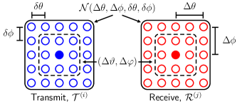
Figure 3: The spatial neighborhoods surrounding a given transmit direction and receive direction (shown as filled circles). The size of the neighborhoods is dictated by ${\left(\Delta\theta,\Delta\phi\right)}$ and their resolution by ${\left(\delta\theta,\delta\phi\right)}$. ${\left(\Delta\vartheta,\Delta\varphi\right)}$ will be relevant in Section VI.

The spatial neighborhoods $\mathcal{T}^{{\left(i^{\star}\right)}}$ and $\mathcal{R}^{{\left(j^{\star}\right)}}$ surrounding the transmit and receive directions output by conventional beam alignment from the previous section are respectively written as

$$\mathcal{T}^{{\left(i^{\star}\right)}} ={\left(\theta_{\mathrm{tx}}^{{\left(i^{\star}\right)}},\phi_{\mathrm{tx}}^{{\left(i^{\star}\right)}}\right)}+\mathcal{N}{\left(\Delta\theta,\Delta\phi,\delta\theta,\delta\phi\right)}$$ (17)

$$\mathcal{R}^{{\left(j^{\star}\right)}} =\underbrace{{\left(\theta_{\mathrm{rx}}^{{\left(j^{\star}\right)}},\phi_{\mathrm{rx}}^{{\left(j^{\star}\right)}}\right)}}_{\mathsf{initial~{}selection}}+\underbrace{\mathcal{N}{\left(\Delta\theta,\Delta\phi,\delta\theta,\delta\phi\right)}}_{\mathsf{neighborhood}}.$$ (18)

The size of these sets is

$${\left|\mathcal{T}^{{\left(i^{\star}\right)}}\right|}={\left|\mathcal{R}^{{\left(j^{\star}\right)}}\right|}={\left|\mathcal{N}{\left(\Delta\theta,\Delta\phi,\delta\theta,\delta\phi\right)}\right|}={\left(2\cdot K_{\theta}+1\right)}\cdot{\left(2\cdot K_{\phi}+1\right)}$$ (19)

where $K_{\theta}=\left\lfloor{\frac{\Delta\theta}{\delta\theta}}\right\rfloor$ and $K_{\phi}=\left\lfloor{\frac{\Delta\phi}{\delta\phi}}\right\rfloor$, indicating that neighborhoods naturally grow with widened ${\left(\Delta\theta,\Delta\phi\right)}$ or finer resolution ${\left(\delta\theta,\delta\phi\right)}$.

When steering its transmit beam toward ${\left(\theta_{\mathrm{tx}},\phi_{\mathrm{tx}}\right)}$ and receive beam toward ${\left(\theta_{\mathrm{rx}},\phi_{\mathrm{rx}}\right)}$, the IAB node incurs an INR of $\mathsf{INR}_{\mathrm{rx}}{\left(\theta_{\mathrm{tx}},\phi_{\mathrm{tx}},\theta_{\mathrm{rx}},\phi_{\mathrm{rx}}\right)}$. In DL-DL mode, $\mathsf{INR}_{\mathrm{rx}}$ can be expressed as

$$\mathsf{INR}_{\mathrm{rx}}{\left(\theta_{\mathrm{tx}},\phi_{\mathrm{tx}},\theta_{\mathrm{rx}},\phi_{\mathrm{rx}}\right)}=\frac{P_{\mathrm{tx}}^{\mathrm{IAB}}\cdot G_{\mathrm{SI}}^{2}\cdot{\left|{\mathbf{w}}{\left(\theta_{\mathrm{rx}},\phi_{\mathrm{rx}}\right)}^{{*}}{\mathbf{H}}_{\mathrm{SI}}{\mathbf{f}}{\left(\theta_{\mathrm{tx}},\phi_{\mathrm{tx}}\right)}\right|}^{2}}{P_{\mathrm{noise}}^{\mathrm{IAB}}}$$ (20)

and that during UL-UL mode can be stated analogously. For each potential initial beam selection ${\left(i^{\star},j^{\star}\right)}$, we propose that the IAB node measure and record $\mathsf{INR}_{\mathrm{rx}}{\left(\theta_{\mathrm{tx}},\phi_{\mathrm{tx}},\theta_{\mathrm{rx}},\phi_{\mathrm{rx}}\right)}$ for all transmit-receive combinations across the neighborhoods $\mathcal{T}^{{\left(i^{\star}\right)}}$ and $\mathcal{R}^{{\left(j^{\star}\right)}}$ to populate

$$\mathcal{I}_{\mathrm{rx}}^{{\left(i^{\star},j^{\star}\right)}} ={\left\{\mathsf{INR}_{\mathrm{rx}}{\left(\theta_{\mathrm{tx}},\phi_{\mathrm{tx}},\theta_{\mathrm{rx}},\phi_{\mathrm{rx}}\right)}:{\left(\theta_{\mathrm{tx}},\phi_{\mathrm{tx}}\right)}\in\mathcal{T}^{{\left(i^{\star}\right)}},{\left(\theta_{\mathrm{rx}},\phi_{\mathrm{rx}}\right)}\in\mathcal{R}^{{\left(j^{\star}\right)}}\right\}}.$$ (21)

The total number of INR measurements collected in $\mathcal{I}_{\mathrm{rx}}^{{\left(i^{\star},j^{\star}\right)}}$ is

$${\left|\mathcal{I}_{\mathrm{rx}}^{{\left(i^{\star},j^{\star}\right)}}\right|} ={\left|\mathcal{T}^{{\left(i^{\star}\right)}}\right|}\cdot{\left|\mathcal{R}^{{\left(j^{\star}\right)}}\right|}={\left(2\cdot K_{\theta}+1\right)}^{2}\cdot{\left(2\cdot K_{\phi}+1\right)}^{2}$$ (22)

which is equal for all $(i^{\star},j^{\star})$ since we have assumed a fixed neighborhood size. This set of receive link INR measurements $\mathcal{I}_{\mathrm{rx}}^{{\left(i^{\star},j^{\star}\right)}}$ will enable the next stage of our proposed design.

Remark 1: Measurement overhead and frequency.

Naturally, conducting these INR measurements at the full-duplex device may become practically prohibitive if the number of measurements grows too large. This depends on the neighborhood size ${\left(\Delta\theta,\Delta\phi\right)}$ and spatial resolution ${\left(\delta\theta,\delta\phi\right)}$, along with how frequently these measurements need to be collected. System engineers can throttle the neighborhood size and/or spatial resolution to reduce the measurement overhead, though this may reduce the effectiveness of Steer, as we will see. In addition to neighborhood size and spatial resolution, the time-variability of self-interference will heavily dictate the overhead of these measurements. In the extreme case, a nearly static self-interference demands infrequent self-interference measurements. Highly dynamic self-interference, on the other hand, will demand more frequent measurements for reliability. Notice that these measurements need not be taken strictly following beam alignment; instead, they can be collected for all $(i,j)$ and referenced for particular $(i^{\star},j^{\star})$, assuming a sufficiently static self-interference channel. In such a case, the set of all INR measurements can be written as $\mathcal{I}_{\mathrm{rx}}=\bigcup_{i=1}^{N_{\mathrm{tx}}}\ \bigcup_{j=1}^{N_{\mathrm{rx}}}\ \mathcal{I}_{\mathrm{rx}}^{{\left(i,j\right)}}$, which has cardinality ${\left|\mathcal{I}_{\mathrm{rx}}\right|}=N_{\mathrm{tx}}\cdot N_{\mathrm{rx}}\cdot{\left(2\cdot K_{\theta}+1\right)}^{2}\cdot{\left(2\cdot K_{\phi}+1\right)}^{2}$ assuming no overlapping transmit neighborhoods or receive neighborhoods. It is important to keep in mind that there is no over-the-air feedback associated with these measurements since they are taken between the transmit and receive panels of the full-duplex IAB node. Reliably measuring $\mathsf{INR}_{\mathrm{rx}}$ is key to the methodology that follows, though small measurement errors would be inherently tolerated; exploring in detail how reliable INR measurements must be would be interesting future work. Note that measuring $\mathsf{INR}_{\mathrm{rx}}$ for some beam pairs may lead to levels of self-interference that saturate the receive chain of the full-duplex transceiver, complicating measurement. It would be valuable future work to develop a means to estimate $\mathsf{INR}_{\mathrm{rx}}$ in such cases (e.g., via transmit power control to avoid saturation), though accuracy would not be especially important, as these beam pairs coupling high self-interference would presumably not be selected by Steer, as we will see.

VI Steer: Joint Transmit-Receive Beam Selection

In this section, we present Steer, our methodology for choosing beams that the IAB node uses to serve the transmit link and receive link. Steer incorporates self-interference during beam selection rather than blindly aiming to maximize SNR, as is typically done in conventional beam alignment. To do so, Steer relies on conventional beam alignment from Section IV to identify the general directions in which beams should be steered. Then, based on some design parameters, transmit and receive beams (${\mathbf{f}}$ and ${\mathbf{w}}$) are jointly selected to serve access and backhaul while simultaneously minimizing the degree of self-interference they couple. This is done by leveraging self-interference measurements taken at the full-duplex IAB node as described in Section V.

Using the initial beam selections ${\left(\theta_{\mathrm{tx}}^{{\left(i^{\star}\right)}},\phi_{\mathrm{tx}}^{{\left(i^{\star}\right)}}\right)}$ and ${\left(\theta_{\mathrm{rx}}^{{\left(j^{\star}\right)}},\phi_{\mathrm{rx}}^{{\left(j^{\star}\right)}}\right)}$ from beam alignment, along with the INR measurements $\mathcal{I}_{\mathrm{rx}}^{{\left(i^{\star},j^{\star}\right)}}$, the objective of Steer is to fetch the transmit beam and receive beam from the neighborhoods $\mathcal{T}^{{\left(i^{\star}\right)}}$ and $\mathcal{R}^{{\left(j^{\star}\right)}}$ that offers full-duplexing gains (in terms of spectral efficiency) over simply using ${\mathbf{f}}{\left(\theta_{\mathrm{tx}}^{{\left(i^{\star}\right)}},\phi_{\mathrm{tx}}^{{\left(i^{\star}\right)}}\right)}$ and ${\mathbf{w}}{\left(\theta_{\mathrm{rx}}^{{\left(j^{\star}\right)}},\phi_{\mathrm{rx}}^{{\left(j^{\star}\right)}}\right)}$ to serve the transmit and receive links. Naturally, when the SNRs of the transmit and receive links are maximized and the interference on each are simultaneously driven to zero, the achievable spectral efficiencies approach their capacities. In pursuit of appreciable $R_{\mathrm{tx}}$ and $R_{\mathrm{rx}}$, we therefore aim to achieve high SNR on each link while reducing interference. However, note that the INR on the transmit link $\mathsf{INR}_{\mathrm{tx}}$ (i.e., cross-link interference) is fixed since we have conditioned on the donor’s beamforming weights. Thus, Steer aims to select ${\mathbf{f}}$ and ${\mathbf{w}}$—the transmit and receive beams at the IAB node—so that high SNR can be achieved on each link while simultaneously reducing self-interference. Note that we do not require the final beam selections output by Steer to be from the codebooks $\mathcal{F}$ and $\mathcal{W}$ but rather will be drawn to steer within $\mathcal{T}^{{\left(i^{\star}\right)}}$ and $\mathcal{R}^{{\left(j^{\star}\right)}}$.

VI-A Target Self-Interference Level

Suppose there exists some target receive link INR threshold $\mathsf{INR}_{\mathrm{rx}}^{\mathrm{tgt}}$ our system desires. For instance, one may choose $\mathsf{INR}_{\mathrm{rx}}^{\mathrm{tgt}}\approx 0$ dB to ensure self-interference does not overwhelmingly exceed noise. Our design that follows does not guarantee that $\mathsf{INR}_{\mathrm{rx}}\leq\mathsf{INR}_{\mathrm{rx}}^{\mathrm{tgt}}$ but rather attempts to meet this target and does not incentivize Steer to provide an $\mathsf{INR}_{\mathrm{rx}}$ further below it. As we will see in our results in Section VIII, choosing a modest $\mathsf{INR}_{\mathrm{rx}}^{\mathrm{tgt}}$ will help Steer yield a more fair and globally optimal solution in terms of sum spectral efficiency since it throttles the sacrifices made in its effort to reduce self-interference. Nonetheless, to force Steer to minimize $\mathsf{INR}_{\mathrm{rx}}$, engineers can use $\mathsf{INR}_{\mathrm{rx}}^{\mathrm{tgt}}=-\infty$ dB.

VI-B Joint Transmit-Receive Beam Selection

Before beginning our design process, we record the receive link INR when steering along the initial beam selections ${\left(\theta_{\mathrm{tx}}^{{\left(i^{\star}\right)}},\phi_{\mathrm{tx}}^{{\left(i^{\star}\right)}}\right)}$ and ${\left(\theta_{\mathrm{rx}}^{{\left(j^{\star}\right)}},\phi_{\mathrm{rx}}^{{\left(j^{\star}\right)}}\right)}$, which we call the nominal receive link INR and express as

$$\mathsf{INR}_{\mathrm{rx}}^{\mathrm{nom}}\triangleq\mathsf{INR}_{\mathrm{rx}}{\left(\theta_{\mathrm{tx}}^{{\left(i^{\star}\right)}},\phi_{\mathrm{tx}}^{{\left(i^{\star}\right)}},\theta_{\mathrm{rx}}^{{\left(j^{\star}\right)}},\phi_{\mathrm{rx}}^{{\left(j^{\star}\right)}}\right)}.$$ (23)

This is the receive link INR incurred if our full-duplex system were to use conventional beam selection and will thus be a useful benchmark to compare against. Desirably, our final beam selections will yield $\mathsf{INR}_{\mathrm{rx}}<\mathsf{INR}_{\mathrm{rx}}^{\mathrm{nom}}$ to make our design worthwhile. Note that if $\mathsf{INR}_{\mathrm{rx}}^{\mathrm{nom}}\leq\mathsf{INR}_{\mathrm{rx}}^{\mathrm{tgt}}$, we need not proceed with our design for this particular ${\left(\theta_{\mathrm{tx}}^{{\left(i^{\star}\right)}},\phi_{\mathrm{tx}}^{{\left(i^{\star}\right)}},\theta_{\mathrm{rx}}^{{\left(j^{\star}\right)}},\phi_{\mathrm{rx}}^{{\left(j^{\star}\right)}}\right)}$ since the target is met inherently by the beams from conventional beam alignment. In such a case, we can simply set the transmit beam and receive beam as ${\mathbf{f}}{\left(\theta_{\mathrm{tx}}^{{\left(i^{\star}\right)}},\phi_{\mathrm{tx}}^{{\left(i^{\star}\right)}}\right)}$ and ${\mathbf{w}}{\left(\theta_{\mathrm{rx}}^{{\left(j^{\star}\right)}},\phi_{\mathrm{rx}}^{{\left(j^{\star}\right)}}\right)}$. When this is not the case, we proceed with our design as follows.

We begin by denoting the minimum INR over the measured spatial neighborhood as

$$\mathsf{INR}_{\mathrm{rx}}^{\mathrm{min}}\triangleq\mathrm{min}{\left(\mathcal{I}_{\mathrm{rx}}^{{\left(i^{\star},j^{\star}\right)}}\right)}.$$ (24)

Then, we form the following beam selection problem to retrieve the transmit direction ${\left(\theta_{\mathrm{tx}}^{\star},\phi_{\mathrm{tx}}^{\star}\right)}$ and receive direction ${\left(\theta_{\mathrm{rx}}^{\star},\phi_{\mathrm{rx}}^{\star}\right)}$ that the full-duplex IAB node will steer toward.

$${\left(\theta_{\mathrm{tx}}^{\star},\phi_{\mathrm{tx}}^{\star}\right)},{\left(\theta_{\mathrm{rx}}^{\star},\phi_{\mathrm{rx}}^{\star}\right)}=\operatorname*{\mathrm{argmin}}_{\begin{subarray}{c}{\left(\theta_{\mathrm{tx}},\phi_{\mathrm{tx}}\right)}\\ {\left(\theta_{\mathrm{rx}},\phi_{\mathrm{rx}}\right)}\end{subarray}} \min_{{\left(\Delta\vartheta,\Delta\varphi\right)}}\ \Delta\vartheta^{2}+\Delta\varphi^{2}$$ (25a)

$$\mathrm{s.t.~{}}\ \mathsf{INR}_{\mathrm{rx}}{\left(\theta_{\mathrm{tx}},\phi_{\mathrm{tx}},\theta_{\mathrm{rx}},\phi_{\mathrm{rx}}\right)}\leq\mathrm{max}{\left(\mathsf{INR}_{\mathrm{rx}}^{\mathrm{tgt}},\mathsf{INR}_{\mathrm{rx}}^{\mathrm{min}}\right)}$$ (25b)

$${\left(\theta_{\mathrm{tx}},\phi_{\mathrm{tx}}\right)}\in{\left(\theta_{\mathrm{tx}}^{{\left(i^{\star}\right)}},\phi_{\mathrm{tx}}^{{\left(i^{\star}\right)}}\right)}+\mathcal{N}{\left(\Delta\vartheta,\Delta\varphi,\delta\theta,\delta\phi\right)}$$ (25c)

$${\left(\theta_{\mathrm{rx}},\phi_{\mathrm{rx}}\right)}\in{\left(\theta_{\mathrm{rx}}^{{\left(j^{\star}\right)}},\phi_{\mathrm{rx}}^{{\left(j^{\star}\right)}}\right)}+\mathcal{N}{\left(\Delta\vartheta,\Delta\varphi,\delta\theta,\delta\phi\right)}$$ (25d)

$$0\leq\Delta\vartheta\leq\Delta\theta,\ 0\leq\Delta\varphi\leq\Delta\phi$$ (25e)

The outer maximization aims to find the transmit and receive steering directions ${\left(\theta_{\mathrm{tx}},\phi_{\mathrm{tx}}\right)}$ and ${\left(\theta_{\mathrm{rx}},\phi_{\mathrm{rx}}\right)}$ that abide by three constraints. First, the steering directions must satisfy (25b), meaning the resulting receive link INR should either be below the desired target $\mathsf{INR}_{\mathrm{rx}}^{\mathrm{tgt}}$ or be the minimum INR offered in the surrounding ${\left(\Delta\theta,\Delta\phi\right)}$-neighborhood (i.e., $\mathsf{INR}_{\mathrm{rx}}^{\mathrm{min}}$). Second, the transmit direction ${\left(\theta_{\mathrm{tx}},\phi_{\mathrm{tx}}\right)}$ should be within the ${\left(\Delta\vartheta,\Delta\varphi\right)}$-neighborhood surrounding the initial transmit beam selection ${\left(\theta_{\mathrm{tx}}^{{\left(i^{\star}\right)}},\phi_{\mathrm{tx}}^{{\left(i^{\star}\right)}}\right)}$, as illustrated in Figure 3. Third, the receive direction ${\left(\theta_{\mathrm{rx}},\phi_{\mathrm{rx}}\right)}$ should be within the ${\left(\Delta\vartheta,\Delta\varphi\right)}$-neighborhood surrounding the initial receive beam selection ${\left(\theta_{\mathrm{rx}}^{{\left(j^{\star}\right)}},\phi_{\mathrm{rx}}^{{\left(j^{\star}\right)}}\right)}$. To constrain the distance of ${\left(\theta_{\mathrm{tx}},\phi_{\mathrm{tx}}\right)}$ from ${\left(\theta_{\mathrm{tx}}^{{\left(i^{\star}\right)}},\phi_{\mathrm{tx}}^{{\left(i^{\star}\right)}}\right)}$ and of ${\left(\theta_{\mathrm{rx}},\phi_{\mathrm{rx}}\right)}$ from ${\left(\theta_{\mathrm{rx}}^{{\left(j^{\star}\right)}},\phi_{\mathrm{rx}}^{{\left(j^{\star}\right)}}\right)}$, we minimize the neighborhood size ${\left(\Delta\vartheta,\Delta\varphi\right)}$ by minimizing $\Delta\vartheta^{2}+\Delta\varphi^{2}$; other distance measures could also be used. Solving this problem will find the transmit and receive steering directions that meet the INR threshold while minimally deviating from those output by conventional beam alignment. In the next section, we present an algorithm for solving problem (25) more efficiently and with fewer INR measurements than an exhaustive search.

Notice that, since $0\leq\Delta\vartheta\leq\Delta\theta$ and $0\leq\Delta\varphi\leq\Delta\phi$, we have

$${\left(\theta_{\mathrm{tx}}^{{\left(i^{\star}\right)}},\phi_{\mathrm{tx}}^{{\left(i^{\star}\right)}}\right)}+\mathcal{N}{\left(\Delta\vartheta,\Delta\varphi,\delta\theta,\delta\phi\right)} \subseteq\mathcal{T}^{{\left(i^{\star}\right)}}$$ (26)

$${\left(\theta_{\mathrm{rx}}^{{\left(j^{\star}\right)}},\phi_{\mathrm{rx}}^{{\left(j^{\star}\right)}}\right)}+\mathcal{N}{\left(\Delta\vartheta,\Delta\varphi,\delta\theta,\delta\phi\right)} \subseteq\mathcal{R}^{{\left(j^{\star}\right)}}$$ (27)

meaning ${\left(\theta_{\mathrm{tx}},\phi_{\mathrm{tx}}\right)}\in\mathcal{T}^{{\left(i^{\star}\right)}}$ and ${\left(\theta_{\mathrm{rx}},\phi_{\mathrm{rx}}\right)}\in\mathcal{R}^{{\left(j^{\star}\right)}}$ for feasible ${\left(\theta_{\mathrm{tx}},\phi_{\mathrm{tx}}\right)}$ and ${\left(\theta_{\mathrm{rx}},\phi_{\mathrm{rx}}\right)}$, and thus $\mathsf{INR}_{\mathrm{rx}}{\left(\theta_{\mathrm{tx}},\phi_{\mathrm{tx}},\theta_{\mathrm{rx}},\phi_{\mathrm{rx}}\right)}\in\mathcal{I}_{\mathrm{rx}}^{{\left(i^{\star},j^{\star}\right)}}$. Hence, solving problem (25) simply requires referencing the receive link INR measurements $\mathcal{I}_{\mathrm{rx}}^{{\left(i^{\star},j^{\star}\right)}}$ to find the transmit direction ${\left(\theta_{\mathrm{tx}}^{\star},\phi_{\mathrm{tx}}^{\star}\right)}$ and receive direction ${\left(\theta_{\mathrm{rx}}^{\star},\phi_{\mathrm{rx}}^{\star}\right)}$ that satisfies the INR target while minimizing the deviation from ${\left(\theta_{\mathrm{tx}}^{{\left(i^{\star}\right)}},\phi_{\mathrm{tx}}^{{\left(i^{\star}\right)}}\right)}$ and ${\left(\theta_{\mathrm{rx}}^{{\left(j^{\star}\right)}},\phi_{\mathrm{rx}}^{{\left(j^{\star}\right)}}\right)}$. After solving this problem, our design concludes by setting the beamforming weights as ${\mathbf{f}}{\left(\theta_{\mathrm{tx}}^{\star},\phi_{\mathrm{tx}}^{\star}\right)}$ and ${\mathbf{w}}{\left(\theta_{\mathrm{rx}}^{\star},\phi_{\mathrm{rx}}^{\star}\right)}$. When transmitting and receiving with these beams output by Steer, we net $\mathsf{SNR}_{\mathrm{tx}}^{\mathrm{ours}}$ and $\mathsf{SNR}_{\mathrm{rx}}^{\mathrm{ours}}$ analogous to those in (12) and a receive link INR of

$$\mathsf{INR}_{\mathrm{rx}}^{\mathrm{ours}} \triangleq\mathsf{INR}_{\mathrm{rx}}{\left(\theta_{\mathrm{tx}}^{\star},\phi_{\mathrm{tx}}^{\star},\theta_{\mathrm{rx}}^{\star},\phi_{\mathrm{rx}}^{\star}\right)}\leq\mathsf{INR}_{\mathrm{rx}}{\left(\theta_{\mathrm{tx}}^{{\left(i^{\star}\right)}},\phi_{\mathrm{tx}}^{{\left(i^{\star}\right)}},\theta_{\mathrm{rx}}^{{\left(j^{\star}\right)}},\phi_{\mathrm{rx}}^{{\left(j^{\star}\right)}}\right)}=\mathsf{INR}_{\mathrm{rx}}^{\mathrm{nom}}.$$ (28)

The receive link INR achieved by Steer is guaranteed to be no more than that with conventional beam selection. Equality in (28) holds when the target $\mathsf{INR}_{\mathrm{rx}}^{\mathrm{tgt}}$ is inherently met by the beams output by beam selection. When this target is not inherently met by initial beam selection, Steer will deviate from the initial steering directions ${\left(\theta_{\mathrm{tx}}^{{\left(i^{\star}\right)}},\phi_{\mathrm{tx}}^{{\left(i^{\star}\right)}}\right)}$ and ${\left(\theta_{\mathrm{rx}}^{{\left(j^{\star}\right)}},\phi_{\mathrm{rx}}^{{\left(j^{\star}\right)}}\right)}$ only if it leads to lower self-interference.

The steering directions output by Steer relative to those from conventional beam selection are bounded as

$${\left|\theta_{\mathrm{tx}}^{\star}-\theta_{\mathrm{tx}}^{{\left(i^{\star}\right)}}\right|},{\left|\theta_{\mathrm{rx}}^{\star}-\theta_{\mathrm{rx}}^{{\left(j^{\star}\right)}}\right|} \leq\Delta\theta,\qquad{\left|\phi_{\mathrm{tx}}^{\star}-\phi_{\mathrm{tx}}^{{\left(i^{\star}\right)}}\right|},{\left|\phi_{\mathrm{rx}}^{\star}-\phi_{\mathrm{rx}}^{{\left(j^{\star}\right)}}\right|}\leq\Delta\phi.$$ (29)

As such, increasing ${\left(\Delta\theta,\Delta\phi\right)}$ may lead to beams that offer lower SNRs since Steer may use beams that are shifted slightly further away from the transmit and receive devices. However, by throttling ${\left(\Delta\theta,\Delta\phi\right)}$ and courtesy of the INR variability observed over small neighborhoods (on the order of one degree), this potential SNR loss can be constrained and may be greatly outweighed by the reduction in INR, netting it an improved SINR over conventional beam selection. Experimental evaluation of Steer in Section VIII confirms this. Note that SNR actually may improve with Steer since it may output beams that are shifted slightly more toward the downlink and uplink devices, compared to those from conventional beam alignment.

Remark 2: Choosing a target self-interference level.

The optimal choice of $\mathsf{INR}_{\mathrm{rx}}^{\mathrm{tgt}}$ (in a sum spectral efficiency sense) cannot be stated analytically since it depends on how much Steer must deviate to meet this target INR, which itself depends on the self-interference channel. In Section VIII, we find an optimal target heuristically, which shows that $\mathsf{INR}_{\mathrm{rx}}^{\mathrm{tgt}}\approx-7$ dB is generally near-optimal in maximizing the sum spectral efficiency achieved by Steer. It is difficult to offer commentary on choosing a suitable $\mathsf{INR}_{\mathrm{rx}}^{\mathrm{tgt}}$ that generalizes to systems beyond the platform we used to evaluate Steer, since each will have a unique self-interference profile.

Remark 3: Design decisions and motivations.

We would now like to comment on some of the design decisions and motivations behind Steer. First, we point out that a more attractive beam selection solution would perhaps be one that maximizes the sum spectral efficiency of the transmit and receive links, rather than minimize the receive link INR as is done by Steer. It is practically implausible to reliably maximize sum spectral efficiency since such a problem requires knowing the SNR achieved by a given beam (which would require prohibitive feedback) or downlink and uplink channel knowledge. Minimizing receive link INR by Steer was chosen deliberately, as it relieves the beam selection problem from requiring SNR knowledge. Instead, Steer solely minimizes self-interference through measurements taken at the IAB node and can preserve SNR by reducing its deviation from those output by conventional beam alignment. We also would like to point out that neighborhood size ${\left(\Delta\theta,\Delta\phi\right)}$ and spatial resolution ${\left(\delta\theta,\delta\phi\right)}$ could be uniquely defined for transmit and receive beam selection, rather than having a common one as we have assumed herein. In cases where transmit and receive beam selection are not executed at the same time (e.g., due to a fixed backhaul link), one could simply condition on the beam not being selected (fixing its steering direction) when running Steer. In cases where Steer cannot offer sufficiently low INR to justify full-duplex operation when serving particular transmit and receive users, there is the potential to serve them instead in a half-duplex fashion.

VII Efficiently Implementing Steer in Real Systems

Having presented its core components, we now present an algorithm for efficiently executing Steer (by which we mean solving problem (25)), along with commentary on key practical considerations. We begin with presentation of Algorithm 1. As it was presented in the previous sections, Steer may be executed by first collecting a set of self-interference measurements and then solving problem (25), presumably by exhaustive search. While this exhaustive search has fairly low computational complexity, the radio resources consumed to conduct self-interference measurements may be a key bottleneck in practical settings. Motivated by this, we now present an algorithm that executes Steer with a minimal number of measurements.

Algorithm 1 begins by sorting all transmit-receive direction pairs $\mathcal{V}=\mathcal{T}^{{\left(i^{\star}\right)}}\times\mathcal{R}^{{\left(j^{\star}\right)}}$ based on their deviation from the nominal directions ${\left(\theta_{\mathrm{tx}}^{{\left(i^{\star}\right)}},\phi_{\mathrm{tx}}^{{\left(i^{\star}\right)}}\right)}$ and ${\left(\theta_{\mathrm{rx}}^{{\left(j^{\star}\right)}},\phi_{\mathrm{rx}}^{{\left(j^{\star}\right)}}\right)}$ output by beam alignment. The indices of this sorting we denote $\mathcal{J}$, and the sorted set of transmit-receive direction pairs we write as ${\left[\mathcal{V}\right]}_{\mathcal{J}}$, which can be precomputed and is fixed for some neighborhood. In other words, the transmit-receive direction pairs in ${\left[\mathcal{V}\right]}_{\mathcal{J}}$ increase in distance from the nominal direction pair. Starting with the nominal direction pair ${\left(\theta_{\mathrm{tx}}^{{\left(i^{\star}\right)}},\phi_{\mathrm{tx}}^{{\left(i^{\star}\right)}}\right)}$ and ${\left(\theta_{\mathrm{rx}}^{{\left(j^{\star}\right)}},\phi_{\mathrm{rx}}^{{\left(j^{\star}\right)}}\right)}$, the INR of each transmit-receive direction pair in ${\left[\mathcal{V}\right]}_{\mathcal{J}}$ is measured until a transmit-receive pair yields a measured $\mathsf{INR}_{\mathrm{rx}}$ less than the target $\mathsf{INR}_{\mathrm{rx}}^{\mathrm{tgt}}$. Once this target is met, the transmit-receive pair is guaranteed to satisfy all constraints of problem (25) and minimizes the distance $\Delta\vartheta^{2}+\Delta\varphi^{2}$, courtesy of our sorting of $\mathcal{V}$. No further measurements are required, having only measured a fraction of the full spatial neighborhood. If no beam pairs meet the threshold, the entire ${\left(\Delta\theta,\Delta\phi\right)}$-neighborhood is measured, with the beam pair offering the lowest INR being selected. Rather than collecting all measurements in $\mathcal{I}_{\mathrm{rx}}^{{\left(i^{\star},j^{\star}\right)}}$ and then exhaustively solving problem (25), Algorithm 1 provides a means to solve problem (25) while collecting measurements. This reduces its computational overhead since its extremely simple logic can be executed while taking measurements, and more importantly, the overhead consumed to collect INR measurements can be dramatically reduced. We illustrate this reduction in measurement overhead in Section VIII using an actual 28 GHz phased array platform.

0:  ${\left(\theta_{\mathrm{tx}}^{{\left(i^{\star}\right)}},\phi_{\mathrm{tx}}^{{\left(i^{\star}\right)}}\right)}$, ${\left(\theta_{\mathrm{rx}}^{{\left(j^{\star}\right)}},\phi_{\mathrm{rx}}^{{\left(j^{\star}\right)}}\right)}$, $\mathcal{T}^{{\left(i^{\star}\right)}}$, $\mathcal{R}^{{\left(j^{\star}\right)}}$, $\mathsf{INR}_{\mathrm{rx}}^{\mathrm{tgt}}$

  $\mathsf{INR}_{\mathrm{rx}}^{\mathrm{min}}=\infty$

  $\mathcal{V}=\mathcal{T}^{{\left(i^{\star}\right)}}\times\mathcal{R}^{{\left(j^{\star}\right)}}$

  $\mathcal{D}_{\vartheta}={\left\{\Delta\vartheta=\mathrm{max}{\left({\left|\theta_{\mathrm{tx}}-\theta_{\mathrm{tx}}^{{\left(i^{\star}\right)}}\right|},{\left|\theta_{\mathrm{rx}}-\theta_{\mathrm{rx}}^{{\left(j^{\star}\right)}}\right|}\right)}:{\left({\left(\theta_{\mathrm{tx}},\phi_{\mathrm{tx}}\right)},{\left(\theta_{\mathrm{rx}},\phi_{\mathrm{rx}}\right)}\right)}\in\mathcal{V}\right\}}$

  $\mathcal{D}_{\varphi}={\left\{\Delta\varphi=\mathrm{max}{\left({\left|\phi_{\mathrm{tx}}-\phi_{\mathrm{tx}}^{{\left(i^{\star}\right)}}\right|},{\left|\phi_{\mathrm{rx}}-\phi_{\mathrm{rx}}^{{\left(j^{\star}\right)}}\right|}\right)}:{\left({\left(\theta_{\mathrm{tx}},\phi_{\mathrm{tx}}\right)},{\left(\theta_{\mathrm{rx}},\phi_{\mathrm{rx}}\right)}\right)}\in\mathcal{V}\right\}}$

  $\mathcal{D}={\left\{\Delta\vartheta^{2}+\Delta\varphi^{2}:\Delta\vartheta\in\mathcal{D}_{\vartheta},\Delta\varphi\in\mathcal{D}_{\varphi}\right\}}$

  ${\left[\sim,\mathcal{J}\right]}=\mathrm{sort}{\left(\mathcal{D},\mathsf{ascend}\right)}$

  for ${\left({\left(\theta_{\mathrm{tx}},\phi_{\mathrm{tx}}\right)},{\left(\theta_{\mathrm{rx}},\phi_{\mathrm{rx}}\right)}\right)}\in{\left[\mathcal{V}\right]}_{\mathcal{J}}$ do

     Measure (or reference) $\mathsf{INR}_{\mathrm{rx}}{\left(\theta_{\mathrm{tx}},\phi_{\mathrm{tx}},\theta_{\mathrm{rx}},\phi_{\mathrm{rx}}\right)}$.

     if $\mathsf{INR}_{\mathrm{rx}}{\left(\theta_{\mathrm{tx}},\phi_{\mathrm{tx}},\theta_{\mathrm{rx}},\phi_{\mathrm{rx}}\right)}<\mathsf{INR}_{\mathrm{rx}}^{\mathrm{min}}$ then

        $\mathsf{INR}_{\mathrm{rx}}^{\mathrm{min}}=\mathsf{INR}_{\mathrm{rx}}{\left(\theta_{\mathrm{tx}},\phi_{\mathrm{tx}},\theta_{\mathrm{rx}},\phi_{\mathrm{rx}}\right)}$

        ${\left(\theta_{\mathrm{tx}}^{\star},\phi_{\mathrm{tx}}^{\star}\right)}={\left(\theta_{\mathrm{tx}},\phi_{\mathrm{tx}}\right)}$

        ${\left(\theta_{\mathrm{rx}}^{\star},\phi_{\mathrm{rx}}^{\star}\right)}={\left(\theta_{\mathrm{rx}},\phi_{\mathrm{rx}}\right)}$

        if $\mathsf{INR}_{\mathrm{rx}}{\left(\theta_{\mathrm{tx}},\phi_{\mathrm{tx}},\theta_{\mathrm{rx}},\phi_{\mathrm{rx}}\right)}\leq\mathsf{INR}_{\mathrm{rx}}^{\mathrm{tgt}}$ then

           Break for-loop; target met; no further measurements required.

        end if

     end if

  end for

  ${\left(\theta_{\mathrm{tx}}^{\star},\phi_{\mathrm{tx}}^{\star}\right)}$, ${\left(\theta_{\mathrm{rx}}^{\star},\phi_{\mathrm{rx}}^{\star}\right)}$

Algorithm 1 Executing Steer by solving problem (25) with a minimal number of measurements.

Remark 4: Practical considerations.

We highlight that the execution of Steer, along with its associated self-interference measurements, take place solely at the full-duplex IAB node. In fact, the donor and user presumably need not be informed of the beams selected by Steer since only the beams at the IAB node are slightly shifted from those output by conventional beam alignment. This is a practically desirable property of Steer. We would also like to emphasize that a practical implementation of Steer is highly dependent on a number of things. First and foremost, it depends heavily on the time-variability of self-interference, which is currently not well investigated. If self-interference is highly dynamic, measurements will need to be collected more frequently and, with updated measurements, Steer will need to be rerun. However, it may be preferable to first re-measure existing Steer solutions to locate ones that may have become stale, no longer offering sufficiently low INR. Note that, when swapping from the DL-DL operating mode to the UL-UL mode, the self-interference measurements may not be symmetric since the panels presumably swap transmit/receive roles, meaning measurements may need to be collected uniquely for each of the two full-duplexing modes. Characterizing the time-variability and reciprocity of self-interference, along with practical implementations of Steer at mmWave frequencies beyond 28 GHz, are good topics for future work.

Remark 5: Precomputing Steer solutions.

With collected measurements and known codebooks $\mathcal{F}$ and $\mathcal{W}$, the IAB node can precompute the solution output by Steer for all possible $(i^{\star},j^{\star})$, keeping a record of ${\left(\theta_{\mathrm{tx}}^{\star},\phi_{\mathrm{tx}}^{\star},\theta_{\mathrm{rx}}^{\star},\phi_{\mathrm{rx}}^{\star}\right)}$ for each. Thereafter, the IAB node can directly map initial beam selection indices to the precomputed solution via a lookup table, rather than re-running Steer. This is another practically desirable property of Steer.

$$(i^{\star},j^{\star})\xrightarrow{\mathsf{lookup}}{\left(\theta_{\mathrm{tx}}^{\star},\phi_{\mathrm{tx}}^{\star},\theta_{\mathrm{rx}}^{\star},\phi_{\mathrm{rx}}^{\star}\right)}$$ (30)

In such a case, the IAB node will need to store $N_{\mathrm{tx}}\cdot N_{\mathrm{rx}}\cdot 4$ values for a given ${\left(\Delta\theta,\Delta\phi\right)}$ and ${\left(\delta\theta,\delta\phi\right)}$. Note that, when the phased arrays are equipped with functions that internally map steering direction to beamforming weights, precomputing Steer solutions only requires storing the steering directions ${\left(\theta_{\mathrm{tx}}^{\star},\phi_{\mathrm{tx}}^{\star}\right)}$, ${\left(\theta_{\mathrm{rx}}^{\star},\phi_{\mathrm{rx}}^{\star}\right)}$ and not the explicit beamforming weights ${\mathbf{f}}^{\star}$ and ${\mathbf{w}}^{\star}$, reducing storage requirements.

Remark 6: Summary of Steer .

A summary of our entire beam selection methodology is illustrated in Figure 2 and is outlined in Algorithm 2. Steer begins by executing conventional beam alignment using codebooks $\mathcal{F}$ and $\mathcal{W}$ to yield initial transmit and receive beam selections that steer toward ${\left(\theta_{\mathrm{tx}}^{{\left(i^{\star}\right)}},\phi_{\mathrm{tx}}^{{\left(i^{\star}\right)}}\right)}$ and ${\left(\theta_{\mathrm{rx}}^{{\left(j^{\star}\right)}},\phi_{\mathrm{rx}}^{{\left(j^{\star}\right)}}\right)}$. Then, based on some defined neighborhood size ${\left(\Delta\theta,\Delta\phi\right)}$ and spatial resolution ${\left(\delta\theta,\delta\phi\right)}$, the spatial neighborhoods surrounding these initial transmit and receive beams are constructed as $\mathcal{T}^{{\left(i^{\star}\right)}}$ and $\mathcal{R}^{{\left(j^{\star}\right)}}$. A receive link INR target $\mathsf{INR}_{\mathrm{rx}}^{\mathrm{tgt}}$ is specified by system engineers, likely based on simulation, experimentation, and field trials. Solving problem (25) via Algorithm 1 will yield the transmit and receive steering directions ${\left(\theta_{\mathrm{tx}}^{\star},\phi_{\mathrm{tx}}^{\star}\right)}$ and ${\left(\theta_{\mathrm{rx}}^{\star},\phi_{\mathrm{rx}}^{\star}\right)}$ that minimally deviate from the initial steering directions while attempting to meet the target INR and minimizing the number of INR measurements collected.

  1. Define transmit and receive coverage regions $\mathcal{A}_{\mathrm{tx}}$ and $\mathcal{A}_{\mathrm{rx}}$ and corresponding transmit and receive codebooks $\mathcal{F}$ and $\mathcal{W}$ for beam alignment.

  2. Conduct conventional beam alignment to yield ${\left(\theta_{\mathrm{tx}}^{{\left(i^{\star}\right)}},\phi_{\mathrm{tx}}^{{\left(i^{\star}\right)}}\right)}$ and ${\left(\theta_{\mathrm{rx}}^{{\left(j^{\star}\right)}},\phi_{\mathrm{rx}}^{{\left(j^{\star}\right)}}\right)}$.

  3. Define the measurement spatial resolution ${\left(\delta\theta,\delta\phi\right)}$ and neighborhood size ${\left(\Delta\theta,\Delta\phi\right)}$.

  4. Construct transmit and receive neighborhoods $\mathcal{T}^{{\left(i^{\star}\right)}}$ and $\mathcal{R}^{{\left(j^{\star}\right)}}$.

  5. Define a desired receive link INR threshold $\mathsf{INR}_{\mathrm{rx}}^{\mathrm{tgt}}$.

  6. Solve problem (25) for ${\left(\theta_{\mathrm{tx}}^{\star},\phi_{\mathrm{tx}}^{\star}\right)}$ and ${\left(\theta_{\mathrm{rx}}^{\star},\phi_{\mathrm{rx}}^{\star}\right)}$ using Algorithm 1, collecting/referencing a minimal number of measurements of self-interference.

  7. Set transmit weights as ${\mathbf{f}}{\left(\theta_{\mathrm{tx}}^{\star},\phi_{\mathrm{tx}}^{\star}\right)}$ and receive weights as ${\mathbf{w}}{\left(\theta_{\mathrm{rx}}^{\star},\phi_{\mathrm{rx}}^{\star}\right)}$.

Algorithm 2 A summary of our beam selection methodology Steer.

VIII Evaluating Steer Through Measurement and Simulation

We experimentally evaluate Steer by combining Monte Carlo simulation with INR measurements taken with a 28 GHz phased array platform. A donor and UE are randomly dropped around an IAB node within simulation [32], followed by beam alignment, and then execution of Steer using actual INR measurements. In other words, $\mathsf{INR}_{\mathrm{rx}}$ values have been measured, while SNR terms are based on simulation. We consider the case where a full-duplex IAB node transmits and receives using panels on two sides of a sectorized triangular platform, as illustrated in Figure 4. The transmit and receive arrays are identical $28$ GHz $16\times 16$ half-wavelength UPAs [33]. Using the platform in Figure 4, we measure $\mathsf{INR}_{\mathrm{rx}}$ as described in Section V using a fixed spatial resolution of ${\left(\delta\theta,\delta\phi\right)}={\left(1^{\circ},1^{\circ}\right)}$; it would be valuable future work would explore finer resolutions. We take measurements in an anechoic chamber to first explore the impacts of the direct coupling between arrays; investigating the effects of reflections off of realistic environments is also a good topic for dedicated future work. We transmit upconverted Zadoff-Chu sequences with 100 MHz of bandwidth and apply correlation-based processing to reliably estimate self-interference well below the noise floor. Our $\mathsf{INR}_{\mathrm{rx}}$ measurements are typically accurate to within $1$ dB, based on validation with high-fidelity test equipment [34] and stepped attenuators [35]. We refer readers to our prior work [28] for more details regarding our measurement methodology, which we also employ herein. We consider identical transmit and receive codebooks comprised of $N_{\mathrm{tx}}=N_{\mathrm{rx}}=105$ narrow beams that span in azimuth from $-56^{\circ}$ to $56^{\circ}$ and in elevation from $-24^{\circ}$ to $24^{\circ}$, each with $8^{\circ}$ spacing. The transmit and receive beams are steered using conjugate beamforming weights (i.e., equal gain/matched filter beamforming), described as ${\mathbf{f}}{\left(\theta_{\mathrm{tx}}^{{\left(i\right)}},\phi_{\mathrm{tx}}^{{\left(i\right)}}\right)}=\mathbf{a}_{\mathrm{tx}}{\left(\theta_{\mathrm{tx}}^{{\left(i\right)}},\phi_{\mathrm{tx}}^{{\left(i\right)}}\right)}$ and ${\mathbf{w}}{\left(\theta_{\mathrm{rx}}^{{\left(j\right)}},\phi_{\mathrm{rx}}^{{\left(j\right)}}\right)}=\mathbf{a}_{\mathrm{rx}}{\left(\theta_{\mathrm{rx}}^{{\left(j\right)}},\phi_{\mathrm{rx}}^{{\left(j\right)}}\right)}$, where $\mathbf{a}_{\mathrm{tx}}{\left(\cdot\right)}$ and $\mathbf{a}_{\mathrm{rx}}{\left(\cdot\right)}$ are the transmit and receive array response vectors. The transmit array radiates at an effective isotropic radiated power (EIRP) of $60$ dBm and the receive array output has a noise floor of $P_{\mathrm{noise}}^{\mathrm{IAB}}=-68$ dBm over $100$ MHz. The transmit and receive beams each have a $3$ dB beamwidth of about $7^{\circ}$. In a Monte Carlo fashion, we randomly drop a donor and UE in the coverage region supplied by our codebooks, from $-60^{\circ}$ to $60^{\circ}$ in azimuth and from $-28^{\circ}$ to $28^{\circ}$ in elevation. We assume the donor and UE are in LOS of the IAB node for simplicity and to more straightforwardly evaluate Steer against conventional beam selection. We make initial beam selections by choosing transmit and receive beams that maximize their SNRs (e.g., exhaustive beam search), though Steer could be applied atop any beam alignment scheme.

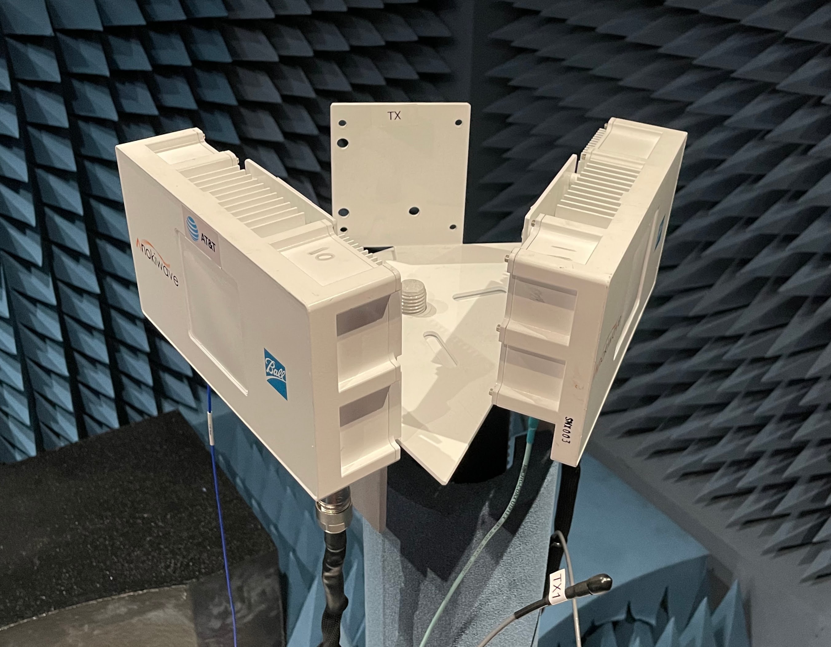
Figure 4: The multi-panel 28 GHz phased array platform used to evaluate Steer through INR measurements. Each phased array is a $16\times 16$ half-wavelength UPA. Measurements were taken in an anechoic chamber, free from significant reflectors.

VIII-A Reducing Measurement Overhead via Algorithm 1

To begin our evaluation of Steer, we first consider Figure 5a, which highlights the reduction in measurements needed when using Algorithm 1 to solve problem (25), compared to measuring the entire spatial neighborhood and then applying exhaustive search. Here, we consider a neighborhood of size ${\left(\Delta\theta,\Delta\phi\right)}={\left(2^{\circ},2^{\circ}\right)}$ with resolution ${\left(\delta\theta,\delta\phi\right)}={\left(1^{\circ},1^{\circ}\right)}$. Figure 5a shows the empirical cumulative density function (CDF) of the fraction of $\mathcal{I}_{\mathrm{rx}}^{{\left(i^{\star},j^{\star}\right)}}$ measured after running Algorithm 1 across all possible $(i^{\star},j^{\star})$. With $\mathsf{INR}_{\mathrm{rx}}^{\mathrm{tgt}}=0$ dB, for instance, nearly $65\%$ of all beam pairs $(i^{\star},j^{\star})$ require at most $20\%$ of the neighborhood to be measured. This highlights the impressive savings Algorithm 1 can offer in terms of measurement overhead, a key practical consideration. Around $12\%$ of beam pairs $(i^{\star},j^{\star})$ require the entire neighborhood $\mathcal{I}_{\mathrm{rx}}^{{\left(i^{\star},j^{\star}\right)}}$ to be measured for $\mathsf{INR}_{\mathrm{rx}}^{\mathrm{tgt}}=0$ dB. With stricter $\mathsf{INR}_{\mathrm{rx}}^{\mathrm{tgt}}$, more measurements are required in order to locate a transmit-receive beam pair that can meet the target. Notice that some fraction of beam pairs require the entire neighborhood to be measured, which is almost exclusively due to the fact that $\mathsf{INR}_{\mathrm{rx}}^{\mathrm{tgt}}$ cannot be met within the neighborhood. In Figure 5b, we show the fraction of beam pairs $(i^{\star},j^{\star})$ that yield each possible ${\left(\Delta\vartheta,\Delta\varphi\right)}$ when ${\left(\Delta\theta,\Delta\phi\right)}={\left(2^{\circ},2^{\circ}\right)}$ and $\mathsf{INR}_{\mathrm{rx}}^{\mathrm{tgt}}=-7$ dB. For example, around $29.5\%$ of beam pairs make use of the full ${\left(2^{\circ},2^{\circ}\right)}$ tolerance allowed. Around $20\%$ of beam pairs reach $\mathsf{INR}_{\mathrm{rx}}\leq-7$ dB with ${\left(1^{\circ},1^{\circ}\right)}$ of shifting.

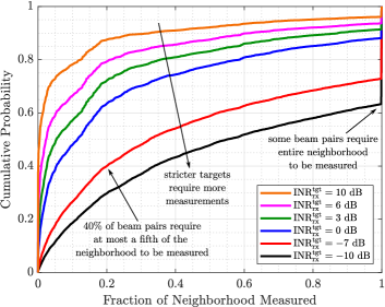
(a) Reducing measurement overhead via Algorithm 1.

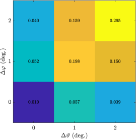
(b) Empirical probability of ${\left(\Delta\vartheta,\Delta\varphi\right)}$.

Figure 5: (a) Illustrating the reduction in measurement overhead necessitated by Steer when using Algorithm 1. $65\%$ of beam pairs only require $20\%$ of measurements to locate a beam pair that meets a target of $\mathsf{INR}_{\mathrm{rx}}^{\mathrm{tgt}}=0$ dB. (b) The empirical probability of the resulting ${\left(\Delta\vartheta,\Delta\varphi\right)}$ after executing Steer on the collected INR measurements for $\mathsf{INR}_{\mathrm{rx}}^{\mathrm{tgt}}=-7$ dB.

VIII-B Performance Metrics

We now introduce performance metrics used to evaluate Steer. Recall, the Shannon capacities of the links we denote $C_{\mathrm{tx}}$ and $C_{\mathrm{rx}}$ are based on the inherent link qualities $\overline{\mathsf{SNR}}_{\mathrm{tx}}$ and $\overline{\mathsf{SNR}}_{\mathrm{rx}}$, respectively. Perhaps more practically meaningful, the capacities of the links after conventional beam alignment we refer to as the codebook capacities, which are

$$C_{\mathrm{tx}}^{\mathrm{cb}} =\mathrm{log}_{2}{\left(1+\mathsf{SNR}_{\mathrm{tx}}^{\mathrm{nom}}\right)}\leq C_{\mathrm{tx}},\quad C_{\mathrm{rx}}^{\mathrm{cb}}=\mathrm{log}_{2}{\left(1+\mathsf{SNR}_{\mathrm{rx}}^{\mathrm{nom}}\right)}\leq C_{\mathrm{rx}}$$ (31)

with these nominal SNRs defined in (12) and the sum codebook capacity as $C_{\mathrm{sum}}^{\mathrm{cb}}=C_{\mathrm{tx}}^{\mathrm{cb}}+C_{\mathrm{rx}}^{\mathrm{cb}}$. Using conventional beam alignment, the achievable sum spectral efficiency of the transmit and receive links under equal time-division duplexing (TDD) with fixed power control (i.e., an instantaneous transmit power constraint) are

$$R_{\mathrm{sum}}^{\mathrm{TDD}}=0.5\cdot\mathrm{log}_{2}{\left(1+\mathsf{SNR}_{\mathrm{tx}}^{\mathrm{nom}}\right)}+0.5\cdot\mathrm{log}_{2}{\left(1+\mathsf{SNR}_{\mathrm{rx}}^{\mathrm{nom}}\right)}.$$ (32)

Under an average power constraint, power control can be used during equal TDD operation to boost transmit power inversely proportional to the transmit duration. In such a case, the sum spectral efficiency becomes

$$R_{\mathrm{sum}}^{\mathrm{TDD}\textrm{-}\mathrm{PC}}=0.5\cdot\mathrm{log}_{2}{\left(1+2\cdot\mathsf{SNR}_{\mathrm{tx}}^{\mathrm{nom}}\right)}+0.5\cdot\mathrm{log}_{2}{\left(1+2\cdot\mathsf{SNR}_{\mathrm{rx}}^{\mathrm{nom}}\right)}.$$ (33)

Note that this achievable sum spectral efficiency coincides with that of equal frequency-division duplexing (FDD). While instantaneous transmit power constraints are more practical, it is still useful for us to compare against an average power constraint to better examine the gains offered by full-duplex. The achievable sum spectral efficiency under Steer we denote as $R_{\mathrm{sum}}^{\mathrm{ours}}=R_{\mathrm{tx}}^{\mathrm{ours}}+R_{\mathrm{rx}}^{\mathrm{ours}}$, which can be computed using (7) with the SINRs achieved by Steer. The achievable sum spectral efficiency under conventional beam selection is defined analogously.

To normalize these achievable sum spectral efficiencies to the sum codebook capacity, we translate them to quantities denoted by $\gamma_{\mathrm{sum}}$ by dividing by $C_{\mathrm{tx}}^{\mathrm{cb}}+C_{\mathrm{rx}}^{\mathrm{cb}}$; for instance, the fraction of the codebook capacity achieved when full-duplexing with Steer is

$$\gamma_{\mathrm{sum}}^{\mathrm{ours}}=\frac{R_{\mathrm{sum}}^{\mathrm{ours}}}{C_{\mathrm{sum}}^{\mathrm{cb}}}=\frac{R_{\mathrm{tx}}^{\mathrm{ours}}+R_{\mathrm{rx}}^{\mathrm{ours}}}{C_{\mathrm{tx}}^{\mathrm{cb}}+C_{\mathrm{rx}}^{\mathrm{cb}}}.$$ (34)

Note that $\gamma_{\mathrm{sum}}$ is typically less than $1$ but is not truly bounded since the codebook capacity is not a true upper bound on achievable spectral efficiency. Nonetheless, codebook capacity is a useful metric since it provides insight on best-case full-duplex performance with a conventional beam codebook (i.e., in the presence of no cross-link or self-interference).

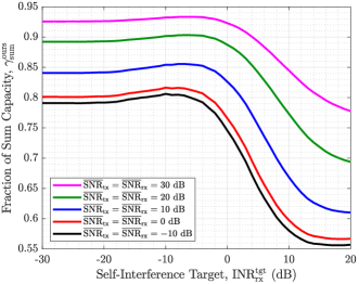
Figure 6: The fraction $\gamma_{\mathrm{sum}}^{\mathrm{ours}}$ of the sum capacity $C_{\mathrm{sum}}^{\mathrm{cb}}$ achieved by Steer as a function of the design parameter $\mathsf{INR}_{\mathrm{rx}}^{\mathrm{tgt}}$ for various $\overline{\mathsf{SNR}}_{\mathrm{tx}}=\overline{\mathsf{SNR}}_{\mathrm{rx}}$. Heuristically, $\mathsf{INR}_{\mathrm{rx}}^{\mathrm{tgt}}=-7$ dB proves to be broadly optimal or near-optimal.

VIII-C Choosing the Receive Link INR Target, $\mathsf{INR}_{\mathrm{rx}}^{\mathrm{tgt}}$.

In Figure 6, we plot the fraction of the sum capacity $\gamma_{\mathrm{sum}}^{\mathrm{ours}}$ achieved by Steer as a function of the design parameter $\mathsf{INR}_{\mathrm{rx}}^{\mathrm{tgt}}$ for various $\overline{\mathsf{SNR}}_{\mathrm{tx}}=\overline{\mathsf{SNR}}_{\mathrm{rx}}$, where we have used ${\left(\Delta\theta,\Delta\phi\right)}={\left(2^{\circ},2^{\circ}\right)}$ and $\mathsf{INR}_{\mathrm{tx}}=0$ dB for this illustration. Heuristically, we observe that the $\mathsf{INR}_{\mathrm{rx}}^{\mathrm{tgt}}$ which maximizes sum spectral efficiency ranges from $-10$ dB to $0$ dB across this broad range of $\overline{\mathsf{SNR}}_{\mathrm{tx}}=\overline{\mathsf{SNR}}_{\mathrm{rx}}$. While choosing $\mathsf{INR}_{\mathrm{rx}}^{\mathrm{tgt}}=-\infty$ dB is near-optimal (especially at high SNR), the optimal $\mathsf{INR}_{\mathrm{rx}}^{\mathrm{tgt}}$ is finite. This is thanks to the fact that choosing a modest $\mathsf{INR}_{\mathrm{rx}}^{\mathrm{tgt}}$ can throttle the deviation that Steer makes from the nominal beams, reducing the chance the donor and/or UE sees low beamforming gain. Henceforth, these numerical results use $\mathsf{INR}_{\mathrm{rx}}^{\mathrm{tgt}}=-7$ dB since it is observed to be optimal or near-optimal broadly across $\overline{\mathsf{SNR}}_{\mathrm{tx}}$ and $\overline{\mathsf{SNR}}_{\mathrm{rx}}$.

VIII-D How Does Full-Duplexing with Steer Compare to Other Multiplexing Strategies?

In Figure 7, we compare full-duplexing with Steer to both half-duplexing and full-duplexing with beams from conventional beam selection. We let ${\left(\Delta\theta,\Delta\phi\right)}={\left(2^{\circ},2^{\circ}\right)}$ with a spatial resolution of ${\left(\delta\theta,\delta\phi\right)}={\left(1^{\circ},1^{\circ}\right)}$ and $\mathsf{INR}_{\mathrm{rx}}^{\mathrm{tgt}}=-7$ dB when running Steer. First, let us examine Figure 7a, which shows the fraction of the sum capacity $\gamma_{\mathrm{sum}}$ achieved by various multiplexing strategies as a function of $\overline{\mathsf{SNR}}_{\mathrm{tx}}=\overline{\mathsf{SNR}}_{\mathrm{rx}}$. (For now, we let $\overline{\mathsf{SNR}}_{\mathrm{tx}}=\overline{\mathsf{SNR}}_{\mathrm{rx}}$ for simplicity and examine $\overline{\mathsf{SNR}}_{\mathrm{tx}}\neq\overline{\mathsf{SNR}}_{\mathrm{rx}}$ shortly.) We aim for the codebook capacity $\gamma_{\mathrm{sum}}=1$ during full-duplex operation, whereas half of this, $\gamma_{\mathrm{sum}}=0.5$, can be achieved via half-duplexing with equal TDD. With TDD-PC, high $\gamma_{\mathrm{sum}}$ can be had at low SNR thanks to $\log{\left(1+x\right)}\approx x$ at low $x$, though these gains diminish toward $0.5$ as SNR increases. Without cross-link interference (when $\mathsf{INR}_{\mathrm{tx}}=-\infty$ dB; shown in black), Steer vastly outperforms TDD across SNRs, achieving $80$% of the codebook capacity at low SNR and over $90$% at high SNR. Albeit less practical, TDD-PC can outperform Steer at low SNR, where doubling SNR approximately doubles spectral efficiency, but falls short for $\overline{\mathsf{SNR}}_{\mathrm{tx}}=\overline{\mathsf{SNR}}_{\mathrm{rx}}\geq 1$ dB. Conventional beam selection also broadly outperforms TDD but only outperforms TDD-PC at $\overline{\mathsf{SNR}}_{\mathrm{tx}}=\overline{\mathsf{SNR}}_{\mathrm{rx}}\geq 13$ dB. The sizable gap between Steer and conventional beam alignment of around $20$% of the codebook capacity is attributed to better self-interference mitigation of Steer. With cross-link interference that is equal to noise (when $\mathsf{INR}_{\mathrm{tx}}=0$ dB; shown in red), we naturally see a drop in performance of both Steer and conventional beam selection. In this case, Steer still broadly outperforms half-duplexing with TDD, while the same cannot be said about conventional beam selection. Rather, attempting to full-duplex with beams from conventional beam selection falls short of TDD for $\overline{\mathsf{SNR}}_{\mathrm{tx}}=\overline{\mathsf{SNR}}_{\mathrm{rx}}\leq 12$ dB. This is due to higher self-interference with conventional beams, which plagues the receive link, and the presence of cross-link interference, which plagues the transmit link. Steer can reduce self-interference to levels that make full-duplex operation worthwhile, even in the presence of cross-link interference.

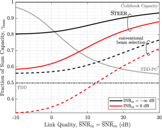
(a) As a function of link quality, $\overline{\mathsf{SNR}}_{\mathrm{tx}}=\overline{\mathsf{SNR}}_{\mathrm{rx}}$.

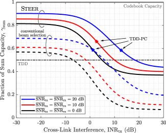
(b) As a function of cross-link interference, $\mathsf{INR}_{\mathrm{tx}}$.

Figure 7: (a) The fraction of the sum capacity $\gamma_{\mathrm{sum}}$ as a function of $\overline{\mathsf{SNR}}_{\mathrm{tx}}=\overline{\mathsf{SNR}}_{\mathrm{rx}}$ for various $\mathsf{INR}_{\mathrm{tx}}$. (b) The fraction of the sum capacity $\gamma_{\mathrm{sum}}$ as a function of $\mathsf{INR}_{\mathrm{tx}}$ for various $\overline{\mathsf{SNR}}_{\mathrm{tx}}=\overline{\mathsf{SNR}}_{\mathrm{rx}}$. $\star$ markers indicate intersections with TDD-PC.

In Figure 7b, we plot the fraction of the sum capacity $\gamma_{\mathrm{sum}}$ achieved by Steer as a function of cross-link interference $\mathsf{INR}_{\mathrm{tx}}$ for various $\overline{\mathsf{SNR}}_{\mathrm{tx}}=\overline{\mathsf{SNR}}_{\mathrm{rx}}$. The starred markers indicate the intersection with performance of TDD-PC. At low cross-link interference, full-duplexing with conventional beam selection outperforms half-duplexing with TDD across SNRs. With Steer, significantly higher spectral efficiencies are obtained largely thanks to its ability to better mitigate self-interference on the receive link. As cross-link interference increases, conventional beam selection degrades as its marginal full-duplexing gains are negated, eventually falling below TDD. At $\overline{\mathsf{SNR}}_{\mathrm{tx}}=\overline{\mathsf{SNR}}_{\mathrm{rx}}=10$ dB, for instance, conventional beam selection can only tolerate $\mathsf{INR}_{\mathrm{tx}}\leq-2$ dB, whereas Steer can tolerate $\mathsf{INR}_{\mathrm{tx}}\leq 10$ dB—a gain of about $12$ dB in robustness to cross-link interference. Here, the rightward and upward shift of Steer compared to conventional beam selection captures its increased robustness to cross-link interference and its improved sum spectral efficiency. Nonetheless, these results emphasize that justifying full-duplex operation with Steer over half-duplexing strategies depends on cross-link interference levels and the inherent transmit and receive link qualities. This motivates the need to study and measure practical cross-link interference levels and routes to mitigate it as needed, potentially via user selection, which may also be used to meet SNR requirements.

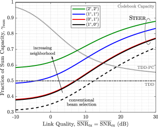
(a) Fraction of the sum capacity, $\gamma_{\mathrm{sum}}$.

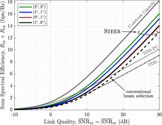
(b) Sum spectral efficiency, $R_{\mathrm{tx}}+R_{\mathrm{rx}}$.

Figure 8: (a) The fraction of the sum capacity $\gamma_{\mathrm{sum}}$ as a function of $\overline{\mathsf{SNR}}_{\mathrm{tx}}=\overline{\mathsf{SNR}}_{\mathrm{rx}}$ for various ${\left(\Delta\theta,\Delta\phi\right)}$, where cross-link interference $\mathsf{INR}_{\mathrm{tx}}=0$ dB. (b) The unnormalized counterpart of (a). Enlarging ${\left(\Delta\theta,\Delta\phi\right)}$ offers noteworthy spectral efficiency gains, especially at high SNR.

VIII-E The Impact of Neighborhood Size ${\left(\Delta\theta,\Delta\phi\right)}$ on Steer’s Peformance

Having examined the performance of Steer versus other multiplexing strategies for a fixed neighborhood size ${\left(\Delta\theta,\Delta\phi\right)}={\left(2^{\circ},2^{\circ}\right)}$, we now inspect its performance for various neighborhood sizes while fixing the spatial resolution to ${\left(\delta\theta,\delta\phi\right)}={\left(1^{\circ},1^{\circ}\right)}$. A larger neighborhood size ${\left(\Delta\theta,\Delta\phi\right)}$ improves Steer’s ability to reduce self-interference since it widens the search space, though this comes at the cost of additional measurement overhead and the potential for gaps in coverage (i.e., reduced SNR). In Figure 8a, we plot the fraction of the sum capacity $\gamma_{\mathrm{sum}}$ achieved by Steer for various ${\left(\Delta\theta,\Delta\phi\right)}$ as a function of $\overline{\mathsf{SNR}}_{\mathrm{tx}}=\overline{\mathsf{SNR}}_{\mathrm{rx}}$, where $\mathsf{INR}_{\mathrm{tx}}=0$ dB. The dashed line shows the performance with conventional beam selection. In Figure 8b, we plot the unnormalized counterpart of Figure 8a (i.e., absolute sum spectral efficiency $R_{\mathrm{tx}}+R_{\mathrm{rx}}$).

Full-duplexing with conventional beam selection offers gains over TDD only beyond SNRs of $12$ dB, which are fairly modest until high SNR. By allowing Steer to shift beams by at most $1^{\circ}$ in azimuth and elevation (i.e., ${\left(\Delta\theta,\Delta\phi\right)}={\left(1^{\circ},1^{\circ}\right)}$), it can choose beams that greatly reduce self-interference to levels such that full-duplex operation matches or significantly outperforms TDD. Notice, with ${\left(1^{\circ},1^{\circ}\right)}$, Steer only requires $\overline{\mathsf{SNR}}_{\mathrm{tx}}=\overline{\mathsf{SNR}}_{\mathrm{rx}}\geq-5$ dB to justify full-duplex operation over TDD. Compared to full-duplexing with conventional beam alignment, this is an SNR gain of over $15$ dB. It is important to realize that this ${\left(1^{\circ},1^{\circ}\right)}$-neighborhood lives well within the $7^{\circ}$ beamwidth of our beams. A gain of about $0.17$ in $\gamma_{\mathrm{sum}}$ is observed with ${\left(1^{\circ},1^{\circ}\right)}$ and this jumps to around $0.27$ with ${\left(2^{\circ},2^{\circ}\right)}$.

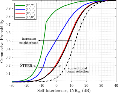
(a) CDF of $\mathsf{INR}_{\mathrm{rx}}$.

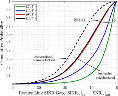
(b) CDF of ${\left[\mathsf{SINR}_{\mathrm{rx}}\right]}_{\mathrm{dB}}-{\left[\overline{\mathsf{SNR}}_{\mathrm{rx}}\right]}_{\mathrm{dB}}$.

Figure 9: (a) The CDF of $\mathsf{INR}_{\mathrm{rx}}$ for various neighborhood sizes ${\left(\Delta\theta,\Delta\phi\right)}$. (b) The CDF of the gap between $\mathsf{SINR}_{\mathrm{rx}}$ and $\overline{\mathsf{SNR}}_{\mathrm{rx}}$ for various neighborhood sizes ${\left(\Delta\theta,\Delta\phi\right)}$. Steer reliably reduces $\mathsf{INR}_{\mathrm{rx}}$, as evident in (a), while maintaining high beamforming gain, shifting $\mathsf{SINR}_{\mathrm{rx}}$ closer to $\overline{\mathsf{SNR}}_{\mathrm{rx}}$ (its upper bound) as shown in (b).

In Figure 9a, we plot the CDF of receive link INR offered by Steer for various neighborhood sizes ${\left(\Delta\theta,\Delta\phi\right)}$. Under conventional beam selection, the INR distribution undesirably lay largely above $0$ dB, where self-interference is stronger than noise. Notice that shifting the transmit and receive beams by at most $1^{\circ}$ in azimuth and elevation, the $\mathsf{INR}_{\mathrm{rx}}$ distribution shifts notably leftward—by about $13$ dB in median. Half of all possible transmit-receive user pairs enjoy an $\mathsf{INR}_{\mathrm{rx}}\leq 0$ dB with Steer when ${\left(\Delta\theta,\Delta\phi\right)}={\left(1^{\circ},1^{\circ}\right)}$. With ${\left(2^{\circ},2^{\circ}\right)}$, almost $90$% of user pairs enjoy $\mathsf{INR}_{\mathrm{rx}}\leq 0$ dB. As a result of using $\mathsf{INR}_{\mathrm{rx}}^{\mathrm{tgt}}=-7$ dB, we see a sharp bend around $\mathsf{INR}_{\mathrm{rx}}=-7$ dB since Steer is not incentivized to reduce the INR below such. Note that there exist select user pairs that require further deviation beyond ${\left(2^{\circ},2^{\circ}\right)}$ in order to deliver low INR. Around $4$% of user pairs see $\mathsf{INR}_{\mathrm{rx}}\geq 10$ dB even with searching for beams across a ${\left(2^{\circ},2^{\circ}\right)}$-neighborhood. Enlarging the neighborhood ${\left(\Delta\theta,\Delta\phi\right)}$ or using a finer spatial resolution ${\left(\delta\theta,\delta\phi\right)}$ may facilitate full-duplexing these user pairs or perhaps they are better off served in a half-duplex fashion.

In Figure 9b, we plot the CDF of the difference in ${\left[\mathsf{SINR}_{\mathrm{rx}}\right]}_{\mathrm{dB}}$ and ${\left[\overline{\mathsf{SNR}}_{\mathrm{rx}}\right]}_{\mathrm{dB}}$ (its upper bound) of Steer for various neighborhood sizes ${\left(\Delta\theta,\Delta\phi\right)}$. This difference is useful in capturing two artifacts of Steer: (i) its reduction in $\mathsf{INR}_{\mathrm{rx}}$ and (ii) its effectiveness in receive beamforming. Recall that $\overline{\mathsf{SNR}}_{\mathrm{rx}}$ is the maximum achievable SNR on the receive link and is only achieved by beamforming directly toward the receive device; a conventional codebook would only achieve this SNR if the receive device was precisely in the direction of one of its receive beams. With conventional beam alignment, $\mathsf{SINR}_{\mathrm{rx}}$ is typically well over $10$ dB short of $\overline{\mathsf{SNR}}_{\mathrm{rx}}$ and is not unlikely to fall over $20$ dB short. When Steer is supplied a ${\left(1^{\circ},1^{\circ}\right)}$-neighborhood, the distribution greatly shifts rightward. Around $40$% of the time, Steer delivers an $\mathsf{SINR}_{\mathrm{rx}}$ that is within $5$ dB of $\overline{\mathsf{SNR}}_{\mathrm{rx}}$. This is thanks to Steer’s ability to reduce $\mathsf{INR}_{\mathrm{rx}}$ and simultaneously deliver high beamforming gain (i.e., high $\mathsf{SNR}_{\mathrm{rx}}$). With ${\left(2^{\circ},2^{\circ}\right)}$, even better performance is delivered by Steer: around $70$% of the time $\mathsf{SINR}_{\mathrm{rx}}$ is within $6$ dB and around $40$% of the time, within $3$ dB. As highlighted before, a tail exists even with a ${\left(2^{\circ},2^{\circ}\right)}$-neighborhood since some user pairs simply cannot be offered low $\mathsf{INR}_{\mathrm{rx}}$ without further deviation (or potentially finer spatial resolution)—a characteristic of the self-interference channel. Due to space constraints, we have omitted an examination of the transmit link. Similar conclusions are drawn: SNR loss is throttled by neighborhood size, as was the motivation behind the design of Steer. It would be valuable future work to investigate how the gains of Steer saturate as the neighborhood ${\left(\Delta\theta,\Delta\phi\right)}$ is widened beyond ${\left(2^{\circ},2^{\circ}\right)}$ or as the resolution ${\left(\delta\theta,\delta\phi\right)}$ is reduced below ${\left(1^{\circ},1^{\circ}\right)}$.

VIII-F For Disparate Transmit and Receive Links

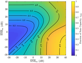
(a) Achieved by conventional beam selection, $\gamma_{\mathrm{sum}}^{\mathrm{nom}}$.

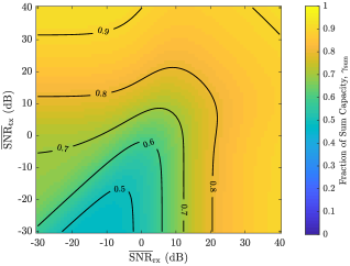
(b) Achieved by Steer, $\gamma_{\mathrm{sum}}^{\mathrm{ours}}$.

Figure 10: The fraction of the sum capacity achieved by (a) conventional beam selection and (b) Steer as a function of ${\left(\overline{\mathsf{SNR}}_{\mathrm{rx}},\overline{\mathsf{SNR}}_{\mathrm{tx}}\right)}$, where $\mathsf{INR}_{\mathrm{tx}}=0$ dB. With Steer, greater sum spectral efficiency is achieved broadly across SNRs, and the region that nets $\gamma\leq 0.5$ (where half-duplexing is preferred) is greatly reduced with Steer.

For our final set of results, we investigate how Steer performs for $\overline{\mathsf{SNR}}_{\mathrm{tx}}\neq\overline{\mathsf{SNR}}_{\mathrm{rx}}$. This is especially important in IAB applications since network-side infrastructure, like fiber-connected donor base stations and IAB nodes, will likely have higher transmit powers, more antennas, and lower noise figures compared to user equipment. In Figure 10a, as a function of $\overline{\mathsf{SNR}}_{\mathrm{tx}}$ and $\overline{\mathsf{SNR}}_{\mathrm{rx}}$, we show the fraction of the sum capacity $\gamma_{\mathrm{sum}}$ achieved when full-duplexing with beams from conventional beam selection, where $\mathsf{INR}_{\mathrm{tx}}=0$ dB. In Figure 10b, we plot that with beams from Steer. Recall that $\gamma_{\mathrm{sum}}=0.5$ can always be achieved by half-duplexing with TDD, meaning we desire full-duplex operation that exceeds this. With conventional beam selection, high $\gamma_{\mathrm{sum}}$ is seen only at high $\overline{\mathsf{SNR}}_{\mathrm{rx}}$, where self-interference is less impactful due to the diminishing gains of $\mathrm{log}_{2}{\left(1+x\right)}$. Notice that, when $\overline{\mathsf{SNR}}_{\mathrm{rx}}\leq 0$ dB, conventional beam selection largely yields $\gamma_{\mathrm{sum}}$ that is worse than TDD for practical $\overline{\mathsf{SNR}}_{\mathrm{tx}}$. When Steer is employed, on the other hand, an obvious improvement can be seen, as higher fractions of the sum capacity are achieved broadly across combinations of $\overline{\mathsf{SNR}}_{\mathrm{tx}}$ and $\overline{\mathsf{SNR}}_{\mathrm{rx}}$. Only a small region at low $\overline{\mathsf{SNR}}_{\mathrm{tx}}$ and low $\overline{\mathsf{SNR}}_{\mathrm{rx}}$ yields $\gamma_{\mathrm{sum}}\leq 0.5$, in which case the system is better off operating using TDD in terms of sum spectral efficiency. Recall these results are with $\mathsf{INR}_{\mathrm{tx}}=0$ dB, meaning they would only improve with reduced cross-link interference.

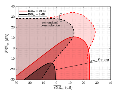
Figure 11: For various cross-link interference levels, the shaded ${\left(\overline{\mathsf{SNR}}_{\mathrm{tx}},\overline{\mathsf{SNR}}_{\mathrm{rx}}\right)}$-region where $\gamma_{\mathrm{sum}}\leq 0.5$ (achieved by equal TDD). This shaded region shrinks dramatically with Steer, outside of which full-duplexing is justified. Steer generally demands lower SNRs to offer gains over half-duplex and can tolerate higher cross-link interference .

Finally, in Figure 11, we compare the ${\left(\overline{\mathsf{SNR}}_{\mathrm{tx}},\overline{\mathsf{SNR}}_{\mathrm{rx}}\right)}$-regions where $\gamma_{\mathrm{sum}}\leq 0.5$ for Steer and for conventional beam selection at various cross-link interference levels. Within the shaded regions, it is advantageous to operate using TDD; outside of them, full-duplexing is worthwhile (i.e., $\gamma_{\mathrm{sum}}\geq 0.5$). When $\mathsf{INR}_{\mathrm{tx}}=0$ dB, the dashed and solid black lines correspond to the $\gamma_{\mathrm{sum}}=0.5$ contours in Figure 10a and Figure 10b, respectively. The region bounded by the solid black line is notably smaller than that bounded by the dashed black line, highlighting the dramatic SNR improvement offered by Steer. At $\overline{\mathsf{SNR}}_{\mathrm{rx}}=-10$ dB, for instance, Steer offers an $\overline{\mathsf{SNR}}_{\mathrm{tx}}$ gain of over $30$ dB. With higher $\mathsf{INR}_{\mathrm{tx}}$, the regions naturally grow as cross-link interference erodes some of the full-duplexing gains. Still, Steer proves to be more robust to cross-link interference as it generally demands lower SNRs to outperform half-duplex.

IX Conclusion

In this work, we present Steer, a measurement-driven beam selection methodology for full-duplex mmWave systems that leverages small shifts of the steering directions of the transmit and receive beams to significantly reduce self-interference and deliver high beamforming gain. Evaluation of Steer through measurements with a 28 GHz phased array platform along with further simulation highlights its ability to reduce self-interference to levels near or below the noise floor, offering noteworthy spectral efficiency gains over half-duplex and full-duplex operation that uses conventional beam selection. Steer can facilitate the deployment of full-duplex mmWave systems to deliver high-throughput, low-latency wireless connectivity, while importantly supporting existing beam alignment schemes in 5G. Valuable future work would include further measuring the time dynamics and small-scale spatial variability of mmWave self-interference, which would ultimately drive design decisions of Steer at deployment. Also, the design of beamforming codebooks that are inherently robust to self-interference and the integration of full-duplex beam selection into mmWave network standards would be useful future contributions. Extending Steer to multi-user/multi-beam systems, along with evaluating Steer using mmWave platforms at other carrier frequencies, in different configurations, and in a variety of settings, would be necessary future work.

References

• [1] T. Riihonen, S. Werner, and R. Wichman, “Mitigation of loopback self-interference in full-duplex MIMO relays,” IEEE Trans. Signal Process., vol. 59, no. 12, pp. 5983–5993, Aug. 2011.
• [2] Z. Xiao, P. Xia, and X. Xia, “Full-duplex millimeter-wave communication,” IEEE Wireless Commun., vol. 24, no. 6, pp. 136–143, Dec. 2017.
• [3] I. P. Roberts, J. G. Andrews, H. B. Jain, and S. Vishwanath, “Millimeter-wave full duplex radios: New challenges and techniques,” IEEE Wireless Commun., pp. 36–43, Feb. 2021.
• [4] E. Everett, C. Shepard, L. Zhong, and A. Sabharwal, “SoftNull: Many-antenna full-duplex wireless via digital beamforming,” IEEE Trans. Wireless Commun., vol. 15, no. 12, pp. 8077–8092, Dec. 2016.
• [5] I. P. Roberts, H. B. Jain, S. Vishwanath, and J. G. Andrews, “Millimeter wave analog beamforming codebooks robust to self-interference,” in Proc. IEEE GLOBECOM, Dec. 2021, pp. 1–6.
• [6] X. Liu, Z. Xiao, L. Bai, J. Choi, P. Xia, and X.-G. Xia, “Beamforming based full-duplex for millimeter-wave communication,” Sensors, vol. 16, no. 7, p. 1130, Jul. 2016.
• [7] R. López-Valcarce and N. González-Prelcic, “Beamformer design for full-duplex amplify-and-forward millimeter wave relays,” in Proc. ISWCS, Aug. 2019, pp. 86–90.
• [8] ——, “Analog beamforming for full-duplex millimeter wave communication,” in Proc. ISWCS, Aug. 2019, pp. 687–691.
• [9] J. Palacios, J. Rodríguez-Fernández, and N. González-Prelcic, “Hybrid precoding and combining for full-duplex millimeter wave communication,” in Proc. IEEE GLOBECOM, Dec. 2019, pp. 1–6.
• [10] K. Satyanarayana, M. El-Hajjar, P. Kuo, A. Mourad, and L. Hanzo, “Hybrid beamforming design for full-duplex millimeter wave communication,” IEEE Trans. Veh. Technol., vol. 68, no. 2, pp. 1394–1404, Feb. 2019.
• [11] L. Zhu, J. Zhang, Z. Xiao, X. Cao, X. Xia, and R. Schober, “Millimeter-wave full-duplex UAV relay: Joint positioning, beamforming, and power control,” IEEE JSAC, vol. 38, no. 9, pp. 2057–2073, Sep. 2020.
• [12] J. M. B. da Silva, A. Sabharwal, G. Fodor, and C. Fischione, “1-bit phase shifters for large-antenna full-duplex mmWave communications,” IEEE Trans. Wireless Commun., vol. 19, no. 10, pp. 6916–6931, Oct. 2020.
• [13] R. López-Valcarce and M. Martínez-Cotelo, “Full-duplex mmWave MIMO with finite-resolution phase shifters,” IEEE Trans. Wireless Commun., May 2022, (early access).
• [14] A. Koc and T. Le-Ngoc, “Full-duplex mmWave massive MIMO systems: A joint hybrid precoding/combining and self-interference cancellation design,” IEEE Open Journal Commun. Society, vol. 2, pp. 754–774, Mar. 2021.
• [15] Y. Cai, Y. Xu, Q. Shi, B. Champagne, and L. Hanzo, “Robust joint hybrid transceiver design for millimeter wave full-duplex MIMO relay systems,” IEEE Trans. Wireless Commun., vol. 18, no. 2, pp. 1199–1215, Feb. 2019.
• [16] I. P. Roberts, J. G. Andrews, and S. Vishwanath, “Hybrid beamforming for millimeter wave full-duplex under limited receive dynamic range,” IEEE Trans. Wireless Commun., vol. 20, no. 12, pp. 7758–7772, Dec. 2021.
• [17] I. P. Roberts, H. B. Jain, and S. Vishwanath, “Equipping millimeter-wave full-duplex with analog self-interference cancellation,” in Proc. IEEE ICC Wkshp., Jun. 2020.
• [18] G. C. Alexandropoulos, M. A. Islam, and B. Smida, “Full duplex hybrid A/D beamforming with reduced complexity multi-tap analog cancellation,” in Proc. IEEE SPAWC, May 2020, pp. 1–5.
• [19] G. C. Alexandropoulos and M. Duarte, “Joint design of multi-tap analog cancellation and digital beamforming for reduced complexity full duplex MIMO systems,” in Proc. IEEE ICC, May 2017, pp. 1–7.
• [20] V. Singh, S. Mondal, A. Gadre, M. Srivastava, J. Paramesh, and S. Kumar, “Millimeter-wave full duplex radios,” in Proc. ACM MobiCom, Apr. 2020.
• [21] C. Zhang and X. Luo, “Adaptive digital self-interference cancellation for millimeter-wave full-duplex backhaul systems,” IEEE Access, vol. 7, pp. 175 542–175 553, Dec. 2019.
• [22] T. Dinc, A. Chakrabarti, and H. Krishnaswamy, “A 60 GHz CMOS full-duplex transceiver and link with polarization-based antenna and RF cancellation,” IEEE J. Solid-State Circuits, vol. 51, no. 5, pp. 1125–1140, May 2016.
• [23] G. Y. Suk, S.-M. Kim, J. Kwak, S. Hur, E. Kim, and C.-B. Chae, “Full duplex integrated access and backhaul for 5G NR: Analyses and prototype measurements,” IEEE Wireless Commun., May 2022, (early access).
• [24] M. Gupta, I. P. Roberts, and J. G. Andrews, “System-level analysis of full-duplex self-backhauled millimeter wave networks,” Dec. 2021. [Online]. Available: https://arxiv.org/abs/2112.05263
• [25] R. W. Heath, N. González-Prelcic, S. Rangan, W. Roh, and A. M. Sayeed, “An overview of signal processing techniques for millimeter wave MIMO systems,” IEEE J. Sel. Topics Signal Process., vol. 10, no. 3, pp. 436–453, Apr. 2016.
• [26] Y. Heng, J. G. Andrews, J. Mo, V. Va, A. Ali, B. L. Ng, and J. C. Zhang, “Six key challenges for beam management in 5.5G and 6G systems,” IEEE Commun. Mag., vol. 59, no. 7, pp. 74–79, Jul. 2021.
• [27] A. Chopra, I. P. Roberts, T. Novlan, and J. G. Andrews, “28 GHz phased array-based self-interference measurements for millimeter wave full-duplex,” in Proc. IEEE WCNC, Apr. 2022, pp. 2583–2588.
• [28] I. P. Roberts, A. Chopra, T. Novlan, S. Vishwanath, and J. G. Andrews, “Beamformed self-interference measurements at 28 GHz: Spatial insights and angular spread,” IEEE Trans. Wireless Commun., (to appear).
• [29] M. Cudak, A. Ghosh, A. Ghosh, and J. G. Andrews, “Integrated access and backhaul: A key enabler for 5G millimeter-wave deployments,” IEEE Commun. Mag., vol. 59, no. 4, pp. 88–94, April 2021.
• [30] C. Dehos, J. L. González, A. D. Domenico, D. Kténas, and L. Dussopt, “Millimeter-wave access and backhauling: the solution to the exponential data traffic increase in 5G mobile communications systems?” IEEE Commun. Mag., vol. 52, no. 9, pp. 88–95, Sep. 2014.
• [31] 3GPP, “3GPP RP-193251: New WID on IAB enhancements,” Dec. 2019. [Online]. Available: https://portal.3gpp.org/ngppapp/CreateTDoc.aspx?mode=view&contributionUid=RP-193251
• [32] I. P. Roberts, “MIMO for MATLAB: A toolbox for simulating MIMO communication systems,” Nov. 2021. [Online]. Available: https://arxiv.org/abs/2111.05273
• [33] “Anokiwave AWA-0134 5G active antenna innovator kit,” 2021. [Online]. Available: https://www.anokiwave.com/products/awa-0134/index.html
• [34] “NRP40SN three path diode power sensor - Rohde & Schwarz,” 2021. [Online]. Available: https://www.rohde-schwarz.com/my/product/nrp40sn-options_63490-160769.html
• [35] “RSC-Z405 RSC step attenuator - Rohde & Schwarz,” 2021. [Online]. Available: https://www.rohde-schwarz.com/us/product/rsc-productstartpage_63493-11395.html