Local resetting with geometric confinement

Abstract

“Local resetting” was recently introduced to describe stochastic resetting in interacting systems where particles independently try to reset to a common “origin”. Our understanding of such systems, where the resetting process is itself affected by interactions, is still very limited. One ubiquitous constraint that is often imposed on the dynamics of interacting particles is geometric confinement, e.g. restricting rigid spherical particles to a channel so narrow that overtaking becomes difficult. We here explore the interplay between local resetting and geometric confinement in a system consisting of two species of diffusive particles: “bath” particles, and “tracers” which undergo local resetting. Mean-field analysis and numerical simulations show that the resetting tracers, whose stationary density profile exhibits a typical “tent-like” shape, imprint this shape onto the bath density profile. Upon varying the ratio of the degree of geometric confinement over particle diffusivity, the system is found to transition between two states. In one tracers expel bath particles away from the origin, while in the other they ensnare them instead. Between these two states, we find a special case where the mean field approximation becomes exact.

Independent Researcher, Haifa 3276605, Israel

1 Introduction

Stochastic resetting is a non-equilibrium process that is typically used to model dynamical observables that are “instantaneously” returned to their initial state some random time after having started their temporal evolution [1, 2, 3, 4, 5, 6, 7, 8, 9]. With applications ranging from search and optimization algorithms [10, 11, 12, 13], through chemical reactions [14, 15, 16], to processes inside biological cells [17, 18, 19], the study of stochastic resetting is attracting broad interest from a diverse scientific audience.

Stochastic resetting has already been vigorously explored under a variety of settings. These efforts have been greatly aided by the “renewal” framework, an analytical tool that allows deriving exact results in situations where stochastic resetting acts “globally” - when stochastic resetting is either applied to a single degree of freedom, or when it is simultaneously applied to multiple degrees of freedom [20, 21, 22, 23, 24]. Perhaps due to its effectiveness and applicability to a wide range of systems, far less attention has been directed towards scenarios where stochastic resetting acts “locally” and the resetting process is itself affected by interactions, i.e. when different interacting degrees of freedom reset independently of one-another. Yet in real complex systems whose dynamics are modeled by stochastic resetting, there is no a-priori reason to assume interactions could not dramatically affect resetting. Exploring the interplay between locally-acting stochastic resetting and various forms of interaction is thus a natural step forward, and a research direction that should be pursued to clarify the nature of stochastic resetting and its consequences.

The “local resetting” process has recently been introduced in an attempt to fill-in this gap [25]. Conditioning the success of a resetting attempt made by one degree of freedom, on the states of all other degrees of freedom has already been applied [25, 26] to study local resetting in a canonical model for interacting systems, the simple exclusion model [27]. Since the renewal approach is limited to global resetting, where all degrees of freedom undergo resetting simultaneously, local resetting is inherently out of its reach. Instead the mean field (MF) approximation was utilized as a means of dealing with the correlations generated by introducing interactions into the resetting process, and interesting observations immediately followed: in the thermodynamic limit and for a fixed particle density, it was shown that the stationary density profile becomes entirely independent of the resetting rate, and that the profile’s shape scales with system size [25]. It was also found that introducing a system-size dependence into the resetting rate has a non-trivial effect on the stationary profile’s shape [25, 26]. Another striking observation, which has yet to be explained, is the existence of parameter regimes where density profiles computed using the MF approximation yield an unexpectedly good fit to direct numerical simulations [25, 26]. Local resetting evidently opens an exciting door to the exploration of the interplay between stochastic resetting and various types of interactions.

One ubiquitous setting which is known to generate non-trivial dynamics in interacting systems is geometric confinement. The prototypical setup for probing the consequence of geometric constraints on the dynamics of interacting systems, is that of diffusive spherical particles with repulsive interactions that are confined to a narrow channel. Geometric confinement and repulsive interactions then typically generate strong spatial and temporal correlations that make it difficult for particles to overtake one-another. The resulting plethora of phenomena, which have been investigated in numerous studies over the past several decades, include tracer sub-diffusion, negative absolute and differential mobility, and the vanishing of the velocity of a driven probe [28, 29, 30, 31, 32, 33, 34, 35, 36, 37, 38, 39, 40, 41, 42, 43, 44, 45, 46]. Following the recent introduction of local resetting, where interactions enter the resetting process, one may wonder: “how would local resetting affect interacting systems whose dynamics are restricted by geometric confinement?”.

Here we study the interplay between stochastic resetting and the geometrically constrained dynamics of interacting diffusive particles. Envision a narrow channel with rigid walls occupied by two species of diffusive spherical particles that interact via short-ranged repulsion. Particles of both species are completely identical except for two properties: 1) each species may have a different mass, and 2) the particles of one of the species undergo local resetting, which here means that an attempt to reset to a target location in the channel is successful only if some fixed volume surrounding the target is vacant of any other particle. Consider particles whose radius is not much smaller than one quarter of the channel’s width, where interactions and geometric confinement conspire to reduce the rate at which neighboring particles overtake one another. Analytically tackling this interacting non-equilibrium system is a very challenging task with current methods and tools. Yet its main ingredients, the interplay between local resetting and geometric constraints, can be studied using a toy model that is more susceptible to analytical treatment. Extending the efforts of [25, 26], we model the narrow channel setup via the stochastic dynamics of hopping particles on a $1D$ ring lattice of $L$ sites. We refer to particles of the species undergoing local resetting as “tracer” particles, while particles of the other species are called “bath” particles. Hard-core exclusion interactions [47, 48, 49], by which particles are excluded from entering an occupied site, replace the channel’s short-ranged repulsive interactions. The different diffusive dynamics of each particle species in the channel, which follow from their mass difference, are modeled by the different rates with which particles attempt to hop into adjacent neighboring lattice sites, setting the tracer hopping rate to $1$ and the bath particle hopping rate to $D$. Tracers also undergo local resetting, independently attempting to reset to the “origin” subject to exclusion. Finally, the geometric confinement imposed by the narrow channel’s walls is modeled by an “overtaking rate” $\varepsilon$, at which a lattice particle attempts to exchange places with a neighboring particle at an adjacent site.

After formulating equations for the evolution of the mean bath and tracer particle density profiles, we apply the MF approximation and compute the profiles in the stationary limit $t\rightarrow\infty$. As in the single species case [25], the stationary tracer density profile $\tau\left(x=\frac{\ell}{L}\right)$ satisfies the same (stationary) evolution equation as a single diffusive particle undergoing stochastic resetting. $\tau\left(x\right)$ correspondingly exhibits the typical “tent-like” shape [1], with a cusp at the origin $x=0$. Yet the main result of this work concerns the behavior of the stationary bath density profile $\rho\left(x\right)$, whose behavior changes dramatically as the ratio $\frac{\varepsilon}{D}$ crosses unity. For $\frac{\varepsilon}{D}<1$ bath particles manage to escape the dense region surrounding the origin, their density profile resembling an inverted tent. But for $\frac{\varepsilon}{D}>1$ bath particles diffuse too slowly to escape and a macroscopic number of them are ensnared near the origin, resulting in a bath density profile whose shape is similar to $\tau\left(x\right)$. When the overtaking and bath hopping rates satisfy $\frac{\varepsilon}{D}=1$, the bath profile becomes flat and equal to $\overline{\rho}$. These three regimes are predicted by MF theory and are validated by direct numerical simulations of the lattice model’s dynamics. While the MF approximation becomes exact at $\varepsilon=D=1$ the agreement between the MF and simulated profiles persists for $\varepsilon\approx D\approx 1$. We hope that the intriguing results that emerge through the interplay of geometric confinement and local resetting will fuel experimental and/or numerical investigations of the narrow channel setup and, more generally, spark interest in how different types of interactions effect the local resetting process.

The paper is organized as follows: Section 2 introduces the $1D$ lattice model used to probe local resetting and geometric confinement in the narrow-channel setup. Our main results, which consist of analytical MF calculations and numerical simulations for the lattice model, are presented in Sec. 3. Section 4 presents the derivation of the evolution equations for the mean bath and tracer density profiles, which contain correlations due to local resetting and geometric confinement. In Sec. 5 we apply the MF approximation to the bath and tracer density profile equations, solve them, and obtain the stationary profiles. The paper is concluded in Sec. 6, where we discuss outstanding open questions and future prospects.

2 The model

We aim to construct a lattice model to describe the dynamics of two species of diffusive spherical particles, locally resetting tracers of mass $m_{t}$ and bath particles of mass $m_{b}$, that are confined to a narrow periodic channel and subject to short-ranged repulsive interactions (right panel of Fig. 1). To this end, consider a $1D$ ring lattice of sites labeled $\ell=0,...,L-1$ occupied by $N$ bath particles and $M$ tracer particles, whose respective mean densities $\overline{\rho}=N/L$ and $\bar{\tau}=M/L$ satisfy $\overline{\rho}+\overline{\tau}\leq 1$. The system evolves in continuous time with the following stochastic dynamics: a bath particle at site $\ell$ attempts hopping to adjacent neighboring sites $\ell+1$ and $\ell-1$ with rate $D$ to each side. Tracer particles similarly attempt hopping to neighboring sites, but with rate $1$ to each side. In addition to hopping, each tracer also tries to reset its position to the “origin” site $\ell=0$ with rate $r$, independently of all other tracers, a process termed “local resetting” in [25]. Two mechanisms mediate interactions between the particles. The first is hard-core “exclusion” [47, 48, 49], by which hopping and resetting attempts that would lead a particle into an occupied site are rejected. Correspondingly, each lattice site can be occupied by one particle at most. The second mechanisms is “exchange”, where a particle at site $\ell$ attempts with rate $\varepsilon$ to exchange sites with a neighboring particle at sites $\ell+1$ and $\ell-1$. The attempt is rejected if the target site is vacant. This mechanism has been previously used to model geometric constraints in similar settings, including the narrow channel setup discussed above [41, 50, 44, 45, 46]. Note that since particles of the same species are indistinguishable, considering exchanges between two particles of the same species is immaterial. Figure 1 provides schematic illustrations of the lattice dynamics (left panel) and the narrow channel setup (right panel).

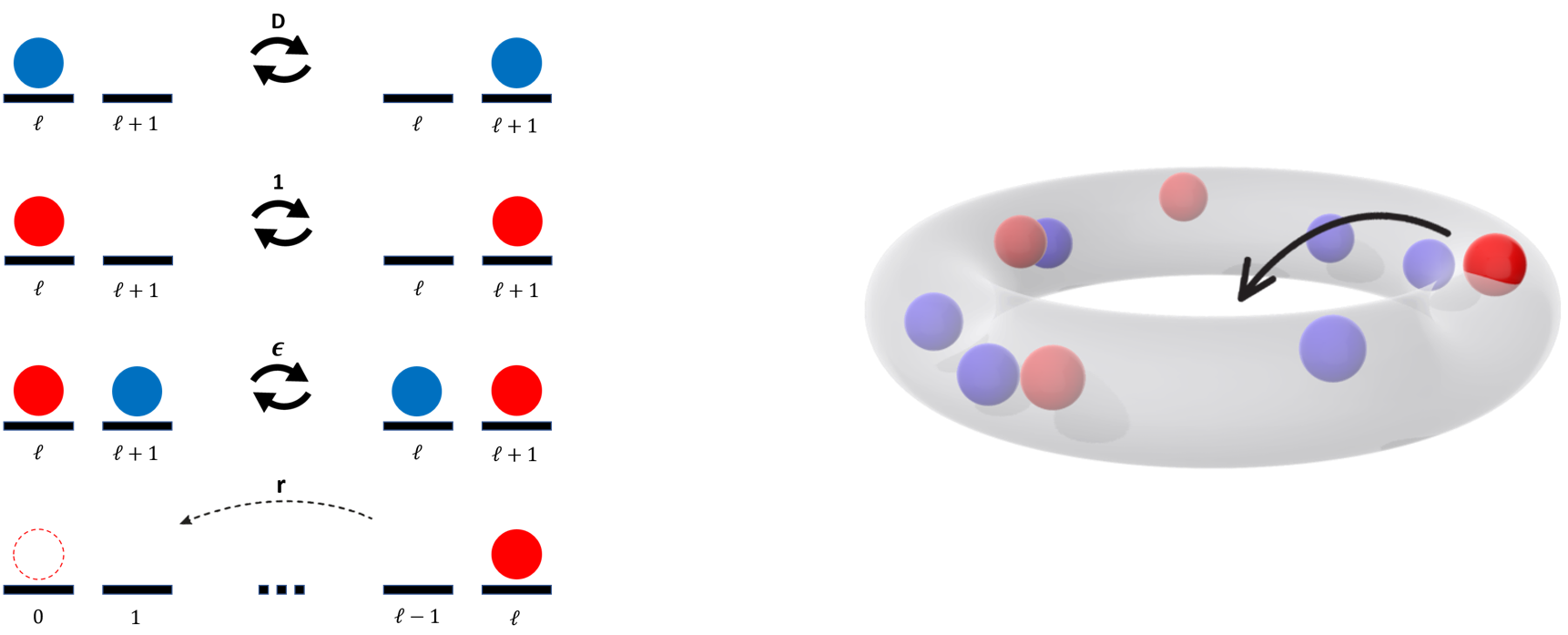
Figure 1: Illustration of the lattice dynamics and the narrow channel setup. Bath particles are depicted in blue and resetting tracers in red. Left: Diagram detailing the $1D$ lattice dynamics. Bath and tracer particles attempt hopping to adjacent sites with rates $D$ and $1$ respectively, exchanges between neighboring particles are attempted with rate $\varepsilon$, and tracers attempt resetting to the origin site $\ell=0$ with rate $r$. Right: Schematic illustration of the narrow channel setup with periodic boundaries, showing a tracer in the midst of a resetting event.

3 Main results

The mean-field (MF) analysis and numerical simulation results presented below demonstrate the non-trivial interplay between local resetting and geometric confinement. In the thermodynamic limit the stationary bath and tracer density profiles, $\rho_{\ell}$ and $\tau_{\ell}$ respectively, are not functions of $\ell$ and $L$ separately but are instead found to depend on the scaling variable $x=\ell/L\in\left[0,1\right)$, i.e. as $L\rightarrow\infty$ we find $\rho_{\ell}\rightarrow\rho\left(x\right)$ and $\tau_{\ell}\rightarrow\tau\left(x\right)$. Moreover, in this limit, the total particle density at the origin approaches unity with finite-size corrections of $\sim\mathcal{O}\left(L^{-2}\right)$. The tracer density profile $\tau\left(x\right)$ is derived using the MF approximation in Eq. (27) and features a tent-like shape with a positive curvature $\tau^{\prime\prime}\left(x\right)>0$ and a cusp at the origin. This can be seen on the right column of Fig. 2, which compares the profiles obtained from MF and numerical simulations for different values of $\varepsilon$ and $D$. We find that, through the combined effect of local resetting and geometric confinement, a simple relation is generated between the bath and tracer profiles (see Eq. (23)), causing the tent-like shape of $\tau\left(x\right)$ to be imprinted on the stationary density profile of the non-resetting bath particles $\rho\left(x\right)$. However, unlike the tracer profile $\tau\left(x\right)$ which retains its shape and curvature for any $\varepsilon,D\neq 0$, the bath profile $\rho\left(x\right)$ transitions between “repelled” and “trapped” states as the value of $\varepsilon/D$ crosses unity (see Eqs. (23) and (27)). For $\varepsilon/D<1$ bath particles are strongly repelled from the dense region near the origin, so that $\rho\left(x\right)$ features a negative curvature $\rho^{\prime\prime}\left(x\right)<0$ and the shape of an inverted tent, as shown in the top left row of Fig. 2. For $\varepsilon/D>1$ a finite fraction of bath particles remain trapped in the dense region surrounding the origin. The left panel in the middle row of Fig. 2 shows that, in this case, $\rho\left(x\right)$ has a positive curvature $\rho^{\prime\prime}\left(x\right)>0$ and a shape similar to that of $\tau\left(x\right)$. At $\varepsilon/D=1$ the bath density profile becomes completely flat, with its value equal to the mean bath density $\overline{\rho}$ (see left panel at the bottom row of Fig. 2). The insets appearing throughout the right column of Fig. 2 plot the difference between the MF and simulated tracer profiles, which is non-zero but still too small to see at scale.

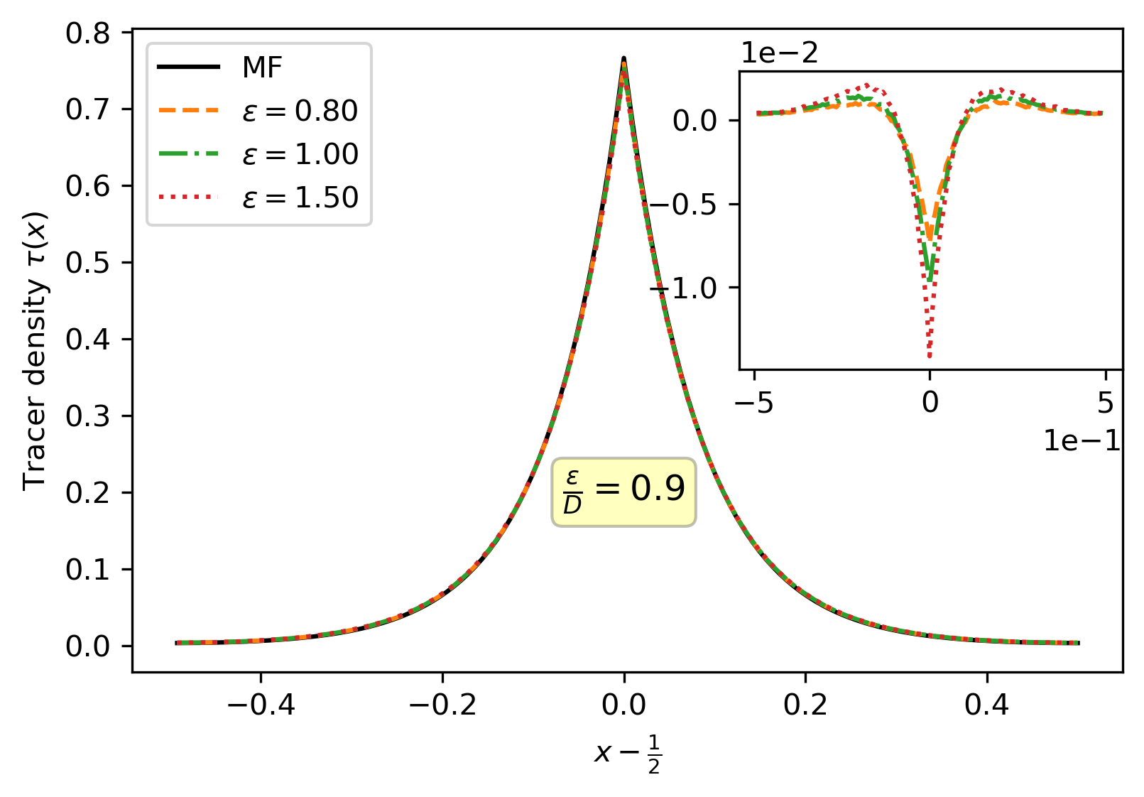
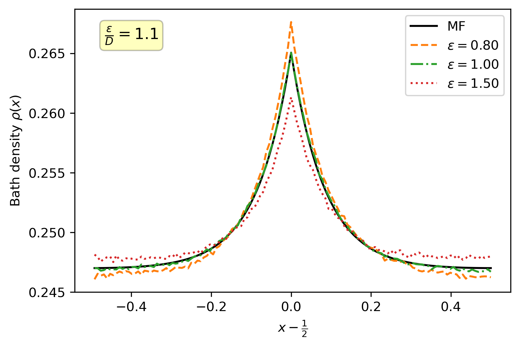
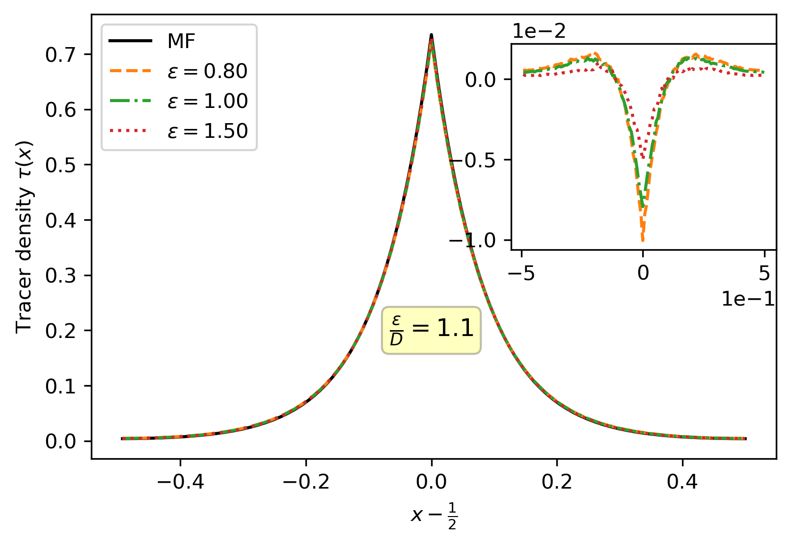
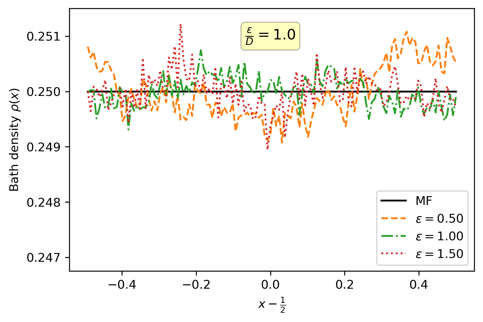
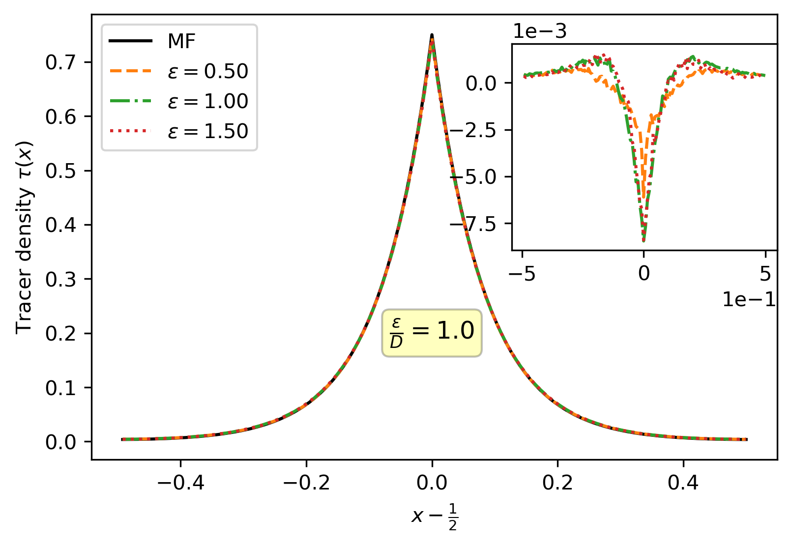
Figure 2: Stationary bath and tracer density profiles for $\overline{\rho}=1/4$, $\overline{\tau}=1/8$, and $r=1$, with a fixed value of $\varepsilon/D$ shown in each row. Notice that the horizontal axis was taken to be $x-1/2$, which simply amounts to shifting the “origin” from $x=0$ to $x=1/2$, to highlight the behavior near the origin. Solid black lines denote the MF profiles, computed in the thermodynamic limit $L\rightarrow\infty$. In this limit Eqs. (23), (27), and (29), show that $\varepsilon$ and $D$ only enter the MF profiles via their ratio $\varepsilon/D$. Dashed, dot-dashed, and dotted lines denote the simulated profiles, obtained for $L=128$ and different values of $\varepsilon$ and $D$.

The different states of $\rho\left(x\right)$ are most easily understood upon fixing the value of the exchange rate $\varepsilon$ to unity, thus setting it equal to the tracer hopping rate. This limit corresponds to a channel that is wide enough for the tracers’ motion to be free of geometric constraints over their diffusive time-scale. We start by considering the repelled state $\varepsilon/D<1$, corresponding to $D>1$. In this state tracers attempt hopping and exchanges with equal rates, but bath particles hop at a higher rate. Imagine a bath particle trapped in the dense region surrounding the origin. Clearly, it has a finite probability to escape the dense region via exchanges with tracers. Once it succeeds in doing so, reaching a region where there is a high density on one side and a low density on the other, the bath particle is more likely to distance itself by hopping away from the origin, rather than to remain stuck therein. The opposite happens in the trapped state $\varepsilon/D>1$ (i.e. $D<1$), where the lower hopping rate implies a bath particle has a higher chance to remain trapped in the dense region near the origin. For $\varepsilon/D=1$ (i.e. $D=1$) the bath particles experience a completely homogeneous environment, since hopping into a vacant site and exchanging sites with a tracer occur with the same rate.

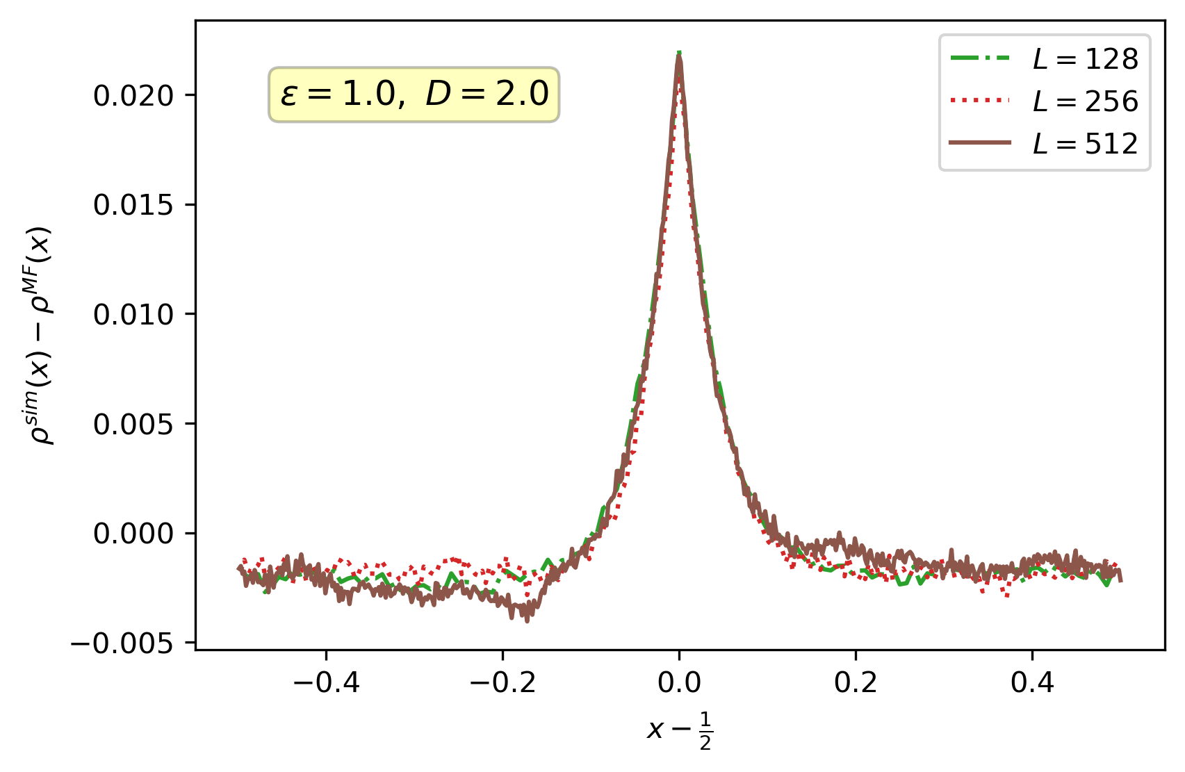
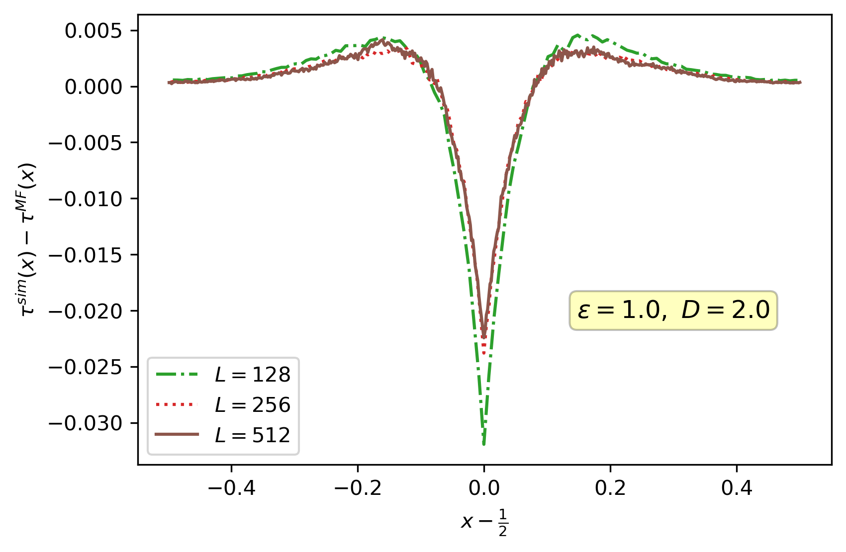
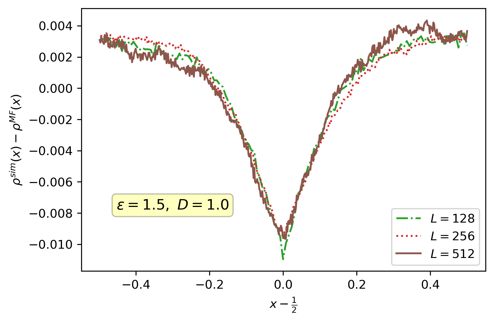
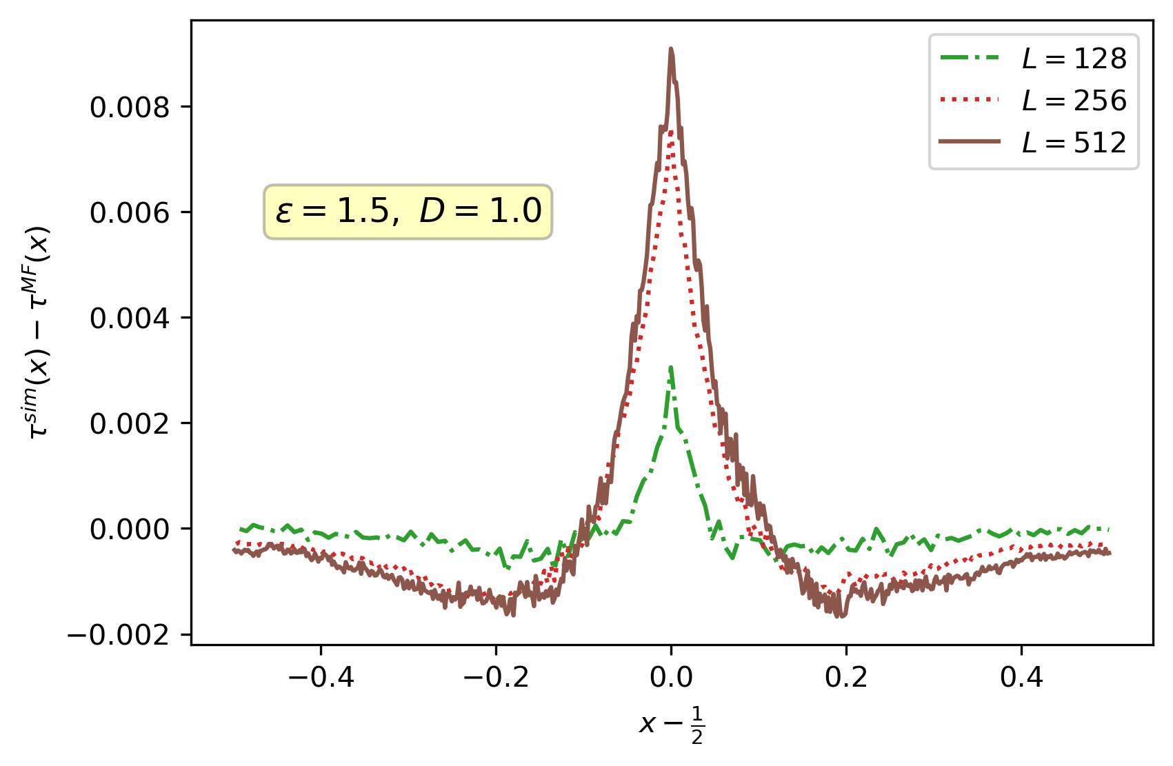
Figure 4: Data collapse of the difference between the simulated and MF profiles for different system sizes $L=128,256,$ and $512$. The parameters $\overline{\rho}=1/4$, $\overline{\tau}=1/8$, and $r=1$ are used throughout with $\varepsilon/D\neq 1$. The first row shows the collapse for $\varepsilon=1$ and $D=2$, while the second row is for $\varepsilon=1.5$ and $D=1$. The collapse implies that the MF and simulated density profiles remain different as $L\rightarrow\infty$. Notice that the horizontal axis is $x-1/2$, which simply amounts to shifting the “origin” from $x=0$ to $x=1/2$.

This leads us to the last main result of this study, which is that the MF stationary density profiles becomes exact for $\varepsilon=D=1$. When substituting $\varepsilon=D=1$ into Eqs. (4) for $\rho\left(x\right)$ and $\tau\left(x\right)$, the correlations due to the overtaking process vanish from both equations. The equation for $\rho\left(x\right)$ becomes effectively decoupled from $\tau\left(x\right)$, and is easily solved to give $\overline{\rho}$, but the remaining equation for $\tau\left(x\right)$ still contains correlations due to the exchange process. For $\varepsilon=D=1$ the MF equation for $\tau\left(x\right)$ is nearly identical to the one studied in [25] for locally resetting particles with exclusion. There, for a fixed particle density and large $L$, the remarkable agreement between the simulated and MF profiles was noted. The same system was later studied numerically in [26], where the MF approximation was suggested to become exact in the limit $L\rightarrow\infty$. Following a numerical investigating the system we here report that for $\varepsilon=D=1$ the MF approximation does indeed seem to become exact in the thermodynamic limit $L\rightarrow\infty$, despite the existence of correlations coming from the local resetting process. Figures 3 and 4 demonstrate this claim by showing data collapse of the difference between the simulated and MF profiles $\delta\rho\left(x\right)\coloneqq\rho^{sim}\left(x\right)-\rho\left(x\right)$ and $\delta\tau\left(x\right)\coloneqq\tau^{sim}\left(x\right)-\tau\left(x\right)$ for different system sizes $L$, with each plot showing data for different values of the parameters $\varepsilon$ and $D$. Data for $\varepsilon/D=1$ is shown in Fig. 3 for $\varepsilon=D=0.1$, for $\varepsilon=D=10$, and for the exact limit $\varepsilon=D=1$. For all parameter sets we find $\delta\rho\left(x\right)\approx 0$, up to structure-less noise due to finite sampling. For $\varepsilon=D=1$ we observe that $L^{2}\times\delta\tau\left(x\right)$ exhibits a convincing data collapse, which suggests that $\delta\tau\left(x\right)\sim\mathcal{O}\left(L^{-2}\right)$ and is consistent with the claim that corrections to MF decay as $L\rightarrow\infty$. Data collapse of $\delta\tau\left(x\right)$ for $\varepsilon=D=10$ and for $\varepsilon=D=0.1$ shows that the correction to MF remain finite as $L\rightarrow\infty$. We complement this picture in Fig. 4, which shows data collapse for $\varepsilon=1$ and $D=2$ (i.e. $\varepsilon/D<1$), and for $\varepsilon=1.5$ and $D=1$ (i.e. $\varepsilon/D>1$). Here the resulting differences $\delta\rho\left(x\right)$ and $\delta\tau\left(x\right)$ are small but also remain finite as $L$ increases. Notice that, as in Fig. 2, the horizontal axis in Figs. 3 and 4 was set to $x-1/2$ to ensure the behavior near the origin is easily and clearly visible.

A final comment about the model parameters is in order. In an effort to isolate the consequence of changing only a subset of the model’s parameters at a time, the figures described above all correspond to the mean bath density $\overline{\rho}=1/8$, mean tracer density $\overline{\tau}=1/4$, and resetting rate $r=1$. Nevertheless, the validity of the entailing results has been confirmed for a variety of mean densities and values of $r$.

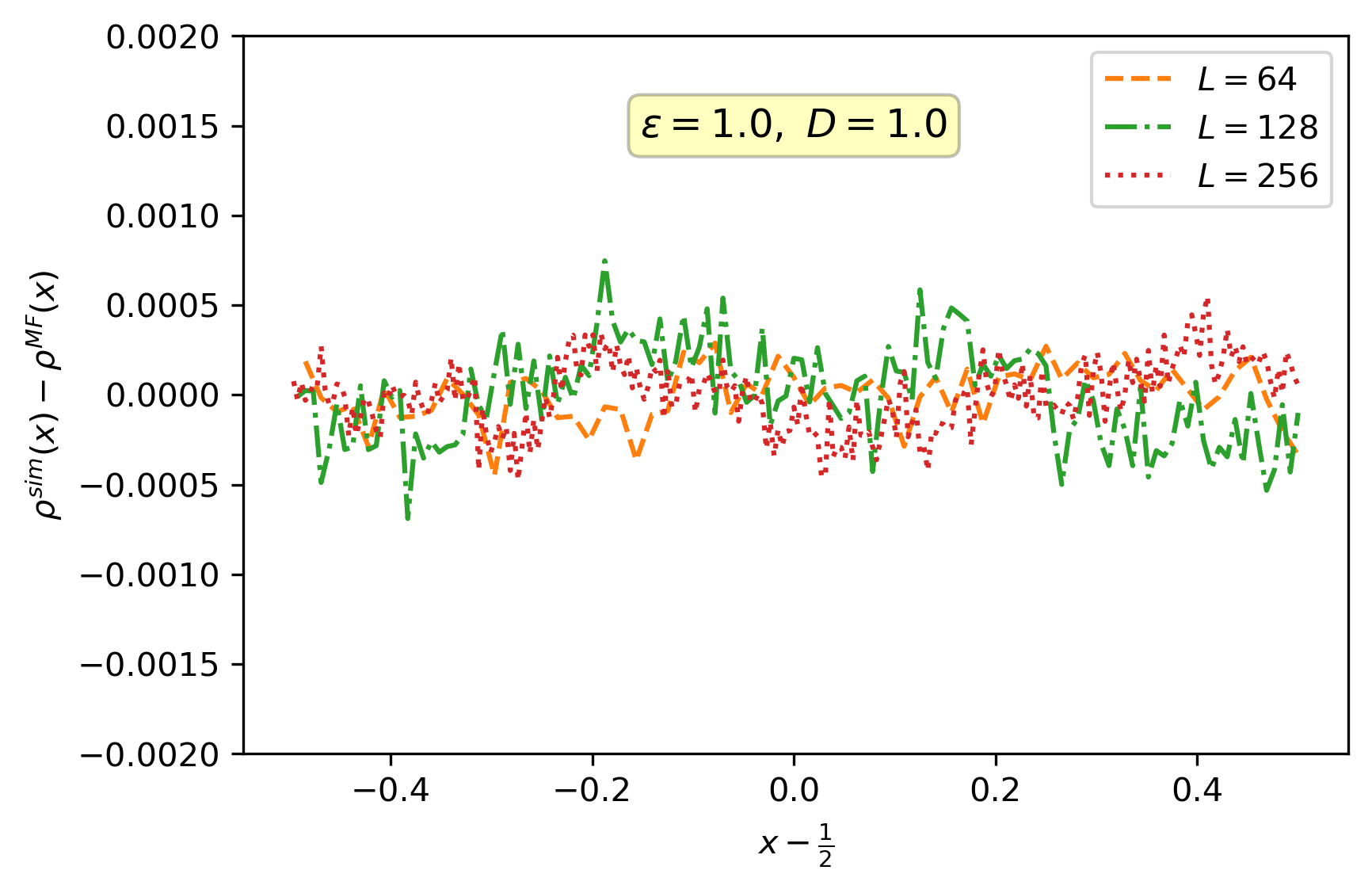
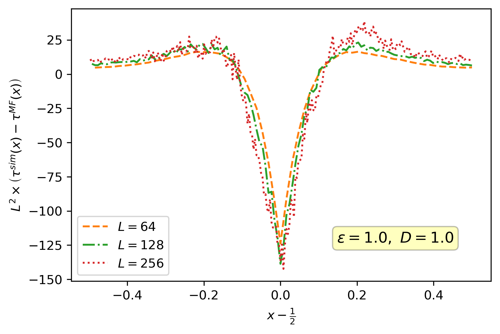
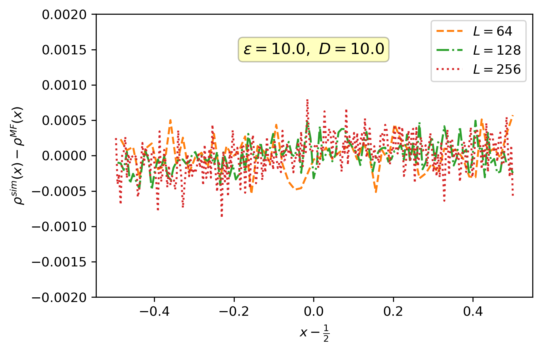
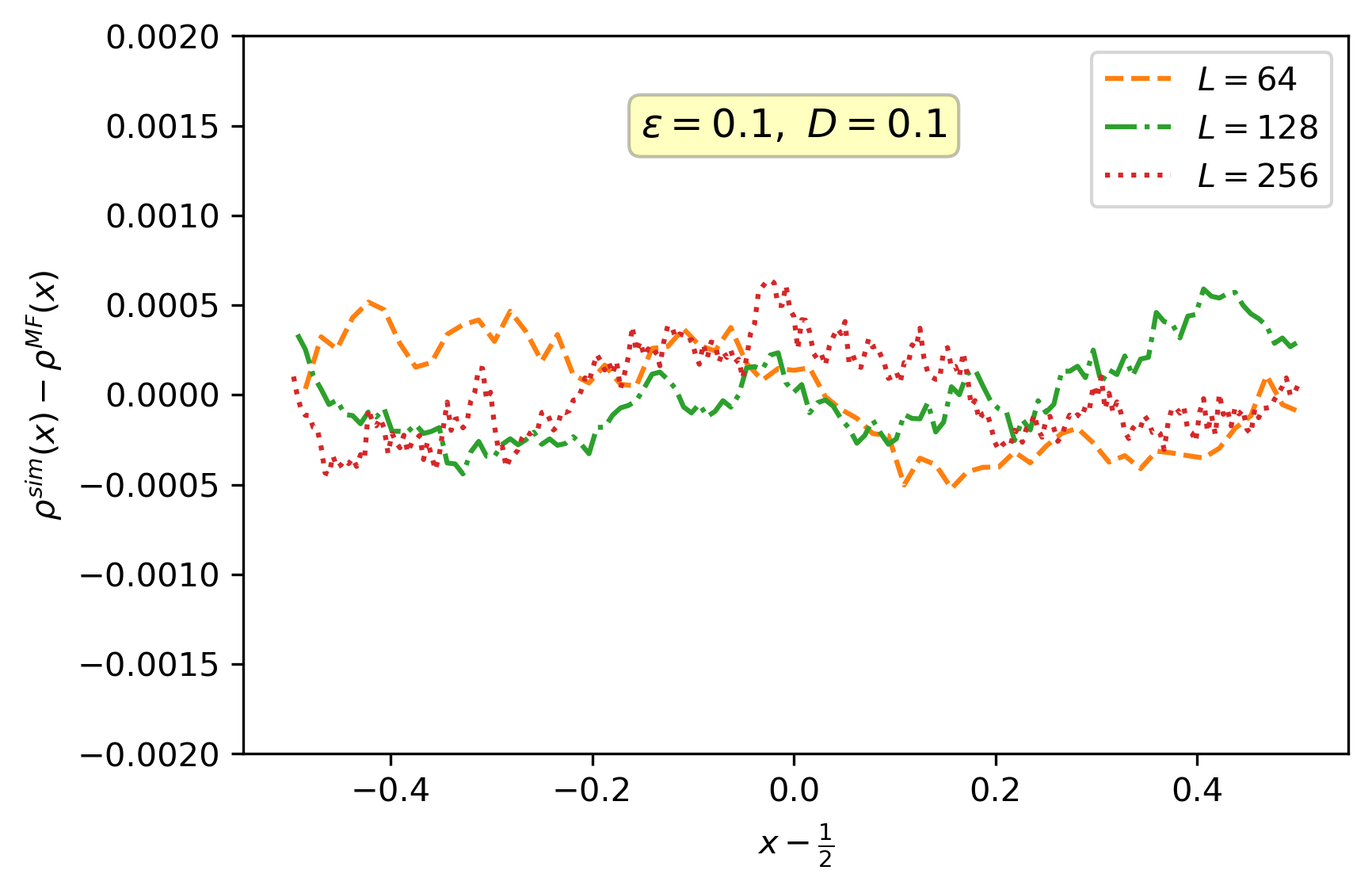
Figure 3: Data collapse of the difference between the simulated and MF profiles for different system sizes $L=64,128,$ and $256$ for the parameters $\overline{\rho}=1/4$, $\overline{\tau}=1/8$, $r=1$, and $\varepsilon/D=1$. Data for the bath and tracers particles is presented on the left and right columns respectively. The first row shows the data collapse for $\varepsilon=D=1$, with the tracer density difference scaled by $L^{2}$, i.e. $L^{2}\delta\tau\left(x\right)$. The convincing collapse for $\varepsilon=D=1$ implies that the MF and simulated tracer density profiles become identical as $L\rightarrow\infty$. For $\varepsilon=D=10$ and $\varepsilon=D=0.1$, shown in the second and third rows, the tracer density difference is not scaled with system size $L$ and the corrections to the MF profiles remain finite. Notice that the horizontal axis is $x-1/2$, which simply amounts to shifting the “origin” from $x=0$ to $x=1/2$.

4 Evolution equations for the mean density profiles

We proceed by formulating the equations governing the evolution of the mean bath and tracer density profiles. Let $\tilde{\rho}_{\ell}\left(t\right)$ denote the instantaneous occupation of site $\ell$ by a bath particle at time $t$, assuming the value $1$ if a bath particle is present and $0$ otherwise, and let $\tilde{\tau}_{\ell}\left(t\right)$ denote the same for tracers. Considering the configurations affecting the occupation of a bath particle at site $\ell$ and averaging over the system’s stochastic dynamics, we obtain an evolution equation for the mean bath density profile $\left\langle\tilde{\rho}_{\ell}\left(t\right)\right\rangle$

$$\partial_{t}\left\langle\tilde{\rho}_{\ell}\right\rangle=D\left\langle\left(1-\tilde{\rho}_{\ell}-\tilde{\tau}_{\ell}\right)\left(\tilde{\rho}_{\ell+1}+\tilde{\rho}_{\ell-1}\right)\right\rangle-D\left\langle\tilde{\rho}_{\ell}\left[\left(1-\tilde{\rho}_{\ell+1}-\tilde{\tau}_{\ell+1}\right)+\left(1-\tilde{\rho}_{\ell-1}-\tilde{\tau}_{\ell-1}\right)\right]\right\rangle$$

$$+\varepsilon\left\langle\tilde{\tau}_{\ell}\left(\tilde{\rho}_{\ell+1}+\tilde{\rho}_{\ell-1}\right)\right\rangle-\varepsilon\left\langle\tilde{\rho}_{\ell}\left(\tilde{\tau}_{\ell+1}+\tilde{\tau}_{\ell-1}\right)\right\rangle.$$ (1)

The first term on the right-hand side describes the bath density gain at site $\ell$ due to configurations where a bath particle at site $\ell\pm 1$ attempts hopping to site $\ell$ with rate $D$. Notice the “exclusion factor” $\left(1-\tilde{\rho}_{\ell}\left(t\right)-\tilde{\tau}_{\ell}\left(t\right)\right)$ weighing this term, which vanishes if site $\ell$ is already occupied by a bath or tracer particle, and is $1$ otherwise. The second term describes the loss of bath density due to the bath particle attempting to leave site $\ell$ by hopping into an adjacent site. The third and fourth terms analogously describe gain and loss terms associated with exchanges between bath and tracer particles, which are attempted with rate $\varepsilon$. The equation for the mean tracer density is

$$\partial_{t}\left\langle\tilde{\tau}_{\ell}\right\rangle=\left\langle\left(\tilde{\tau}_{\ell+1}+\tilde{\tau}_{\ell-1}\right)\left(1-\tilde{\rho}_{\ell}-\tilde{\tau}_{\ell}\right)\right\rangle-\left\langle\tilde{\tau}_{\ell}\left[\left(1-\tilde{\rho}_{\ell+1}-\tilde{\tau}_{\ell+1}\right)+\left(1-\tilde{\rho}_{\ell-1}-\tilde{\tau}_{\ell-1}\right)\right]\right\rangle$$

$$+\varepsilon\left\langle\tilde{\rho}_{\ell}\left(\tilde{\tau}_{\ell+1}+\tilde{\tau}_{\ell-1}\right)\right\rangle-\varepsilon\left\langle\tilde{\tau}_{\ell}\left(\tilde{\rho}_{\ell+1}+\tilde{\rho}_{\ell-1}\right)\right\rangle+\tilde{\chi}_{\ell},$$ (2)

and its construction is analogous to that of Eq. (1). The two equations have nearly the same structure, with the exception of the last term $\tilde{\chi}_{\ell}$ on the right-hand side of Eq. (2). This term, which describes the local resetting of tracers

$$\tilde{\chi}_{\ell}=\begin{cases}\sum_{n=1}^{L-1}r\left\langle\left(1-\tilde{\rho}_{0}-\tilde{\tau}_{0}\right)\tilde{\tau}_{n}\right\rangle&\ell=0\\ -r\left\langle\left(1-\tilde{\rho}_{0}-\tilde{\tau}_{0}\right)\tilde{\tau}_{\ell}\right\rangle&\ell\neq 0\end{cases},$$ (3)

behaves differently at site $\ell=0$ versus sites $\ell\neq 0$: $\tilde{\chi}_{\ell=0}$ is a gain term at site $\ell=0$ that accounts for the attempts made by tracers, located anywhere besides the origin, to reset their position to the origin with rate $r$, whereas $\tilde{\chi}_{\ell\neq 0}$ describes the loss of tracer density at sites $\ell\neq 0$ due to resetting attempts with rate $r$. The exclusion factor $\left(1-\tilde{\rho}_{0}-\tilde{\tau}_{0}\right)$ in $\tilde{\chi}_{\ell}$ ensures that resetting attempts are rejected if the origin is occupied.

Defining the lattice Laplacian $\nabla_{\ell}^{2}$ and gradient $\nabla_{\ell}$ operators, which act on a lattice variable $u_{\ell}$ as $\nabla_{\ell}^{2}u_{\ell}=u_{\ell+1}-2u_{\ell}+u_{\ell-1}$ and $\nabla_{\ell}u_{\ell}=u_{\ell}-u_{\ell-1}$, and respectively denoting the average bath and tracer density profiles by $\rho_{\ell}=\left\langle\tilde{\rho}_{\ell}\right\rangle$ and $\tau_{\ell}=\left\langle\tilde{\tau}_{\ell}\right\rangle$ simplifies Eqs. (1) and (2) to

$$\frac{1}{D}\partial_{t}\rho_{\ell}=\nabla_{\ell}^{2}\rho_{\ell}+\left(1-\frac{\varepsilon}{D}\right)\nabla_{\ell}\left(\left\langle\tilde{\rho}_{\ell}\tilde{\tau}_{\ell+1}\right\rangle-\left\langle\tilde{\tau}_{\ell}\tilde{\rho}_{\ell+1}\right\rangle\right),$$ (4)

and

$$\partial_{t}\tau_{\ell}=\nabla_{\ell}^{2}\tau_{\ell}-\left(1-\varepsilon\right)\nabla_{\ell}\left(\left\langle\tilde{\rho}_{\ell}\tilde{\tau}_{\ell+1}\right\rangle-\left\langle\tilde{\tau}_{\ell}\tilde{\rho}_{\ell+1}\right\rangle\right)+\tilde{\chi}_{\ell}.$$ (5)

It is now apparent that the mean density profiles $\rho_{\ell}$ and $\tau_{\ell}$ are affected by correlations that separate into two contributions: “exchange correlations”, which appear in the second term on the right-hand sides of both equations and are generated by the exchange interactions, and “local resetting” correlations, which only enter Eq. (5) via $\tilde{\chi}_{\ell}$ and are generated by the local resetting process. Particle conservation places an additional constraint on $\rho_{\ell}$ and $\tau_{\ell}$, requiring that

$$\sum_{\ell=0}^{L-1}\rho_{\ell}\left(t\right)=N\text{ and }\sum_{\ell=0}^{L-1}\tau_{\ell}\left(t\right)=M.$$ (6)

Notice that the exchange correlations vanish from both equations for $\varepsilon=D=1$. In this case at sites $\ell\neq 0$ (in the “bulk” of the system) Eqs. (4) and (5) reduce to

$$\partial_{t}\rho_{\ell}=\nabla_{\ell}^{2}\rho_{\ell},$$ (7)

and

$$\partial_{t}\tau_{\ell}=\nabla_{\ell}^{2}\tau_{\ell}-r\left\langle\left(1-\tilde{\rho}_{0}-\tilde{\tau}_{0}\right)\tilde{\tau}_{\ell}\right\rangle,$$ (8)

where the last term in the $\tau_{\ell}$ equation comes from Eq. (3) for $\ell\neq 0$. With the effect of correlations eliminated from Eq. (7) for $\rho_{\ell}$, we can now solve it independently of Eq. (8) for $\tau_{\ell}$. Imposing periodic boundary conditions and bath particle number conservation $\sum_{\ell=0}^{L-1}\rho_{\ell}=N$ yields the stationary solution $\overline{\rho}$. Equation (8) for $\tau_{\ell}$ is nearly identical to the one considered in [25], which studied identical particles undergoing diffusion and local resetting. For a finite particle density and large $L$, the stationary density profile obtained there using the MF approximation was found to be remarkably similar to the empirical profile obtained via numerical simulations of the model’s dynamics, a result which was later validated in [26]. Together with the support provided by the numerical evidence presented in Sec. 3, when local resetting is the only source for correlations, as in Eqs. (8) and (7), the MF approximation seems to become exact in the thermodynamic limit. Applying the MF approximation to the “full” Eqs. (7) and (8), which contain general overtaking rates and general bath and tracer diffusion rates, is correspondingly expected to provide an increasingly accurate description of the model as $\varepsilon,D\rightarrow 1$. We comment that for $\varepsilon=1$ but a general $D\neq 1$, Eq. (5) still contains correlations between the tracer occupation at site $\ell$ and the bath occupation at the origin.

5 Stationary mean-field profiles for general $\varepsilon$ and $D$

Equations (4) and (5) for the average density profiles $\rho_{\ell}$ and $\tau_{\ell}$ involve correlations between the instantaneous particle occupations. These pair of equations are actually the first members of an extensive hierarchy of partial difference equations for all moments of the full $N$ bath particle and $M$ tracer particle distribution, which one would have to formulate and solve to rigorously account for the effect of interactions between the particles on the density profiles. Unfortunately, this hierarchy quickly becomes intractable and there are only a handful of models for which exact methods are known to apply [51, 52]. To make progress we thus resort to the MF approximation, which essentially sets all cumulants to zero, so that $n$-point correlations factorize into products (e.g. $2$-point functions become $\left\langle\tilde{u}_{n}\tilde{v}_{m}\right\rangle\rightarrow\left\langle\tilde{u}_{n}\right\rangle\left\langle\tilde{v}_{\ell}\right\rangle$). Applying the MF approximation to Eqs. (4) and (5) yields

$$\frac{1}{D}\partial_{t}\rho_{\ell}=\nabla_{\ell}^{2}\rho_{\ell}+\left(1-\frac{\varepsilon}{D}\right)\nabla_{\ell}\left(\rho_{\ell}\tau_{\ell+1}-\tau_{\ell}\rho_{\ell+1}\right),$$ (9)

and

$$\partial_{t}\tau_{\ell}=\nabla_{\ell}^{2}\tau_{\ell}-\left(1-\varepsilon\right)\nabla_{\ell}\left(\rho_{\ell}\tau_{\ell+1}-\tau_{\ell}\rho_{\ell+1}\right)+\chi_{\ell},$$ (10)

where $\tilde{\chi}_{\ell}$ in Eq. (5) is replaced by

$$\chi_{\ell}=\begin{cases}\sum_{n=1}^{L-1}r\left(1-\rho_{0}-\tau_{0}\right)\tau_{n}&\ell=0\\ -r\left(1-\rho_{0}-\tau_{0}\right)\tau_{\ell}&\ell\neq 0\end{cases}.$$ (11)

Despite the apparent crudeness of uncontrollably factorizing correlations, as shown in Sec. 3, comparing the MF solutions to numerical simulation results suggest that MF effectively captures the salient features arising from the interplay between geometrically constrained diffusion and local resetting (at least) in the stationary limit $t\rightarrow\infty$. That said, we shall henceforth focus our attention on the model’s stationary density profiles.

We seek solutions for the stationary density profiles of the form $\rho_{\ell}\cong\rho\left(x\right)$ and $\tau_{\ell}\cong\tau\left(x\right)$, where $x=\ell/L\in\left[0,1\right)$ denotes the macroscopic distance and $\cong$ is used to denoted asymptotic equality in the thermodynamic limit $L\rightarrow\infty$. If such solutions exist for all values of the problem’s parameters and satisfy the boundary conditions, they are the unique solutions of the problem. We shall thus self-consistently assume this scaling. Expanding out terms of the form

$$u_{\ell\pm 1}=u\left(x\right)+\frac{1}{L}\partial_{x}u\left(x\right)+\frac{1}{2L^{2}}\partial_{x}^{2}u\left(x\right)+\mathcal{O}\left(L^{-3}\right),$$ (12)

while keeping the leading order behavior in large $L$, yields the stationary bath density equation

$$0=\partial_{x}^{2}\rho+\left(1-\frac{\varepsilon}{D}\right)\left(\rho\partial_{x}^{2}\tau-\tau\partial_{x}^{2}\rho\right),$$ (13)

and the stationary tracer density equation

$$0=\partial_{x}^{2}\tau-\left(1-\varepsilon\right)\left(\rho\partial_{x}^{2}\tau-\tau\partial_{x}^{2}\rho\right)-rL^{2}\left(1-\rho_{0}-\tau_{0}\right)\tau.$$ (14)

It is interesting to notice that Eq. (14) can only be affected by local resetting, diffusion, and exchange processes if $\left(1-\rho_{0}-\tau_{0}\right)\propto L^{-2}$ as $L\rightarrow\infty$, as was previously noted and discussed in [25]. Otherwise, the only contribution to $\tau$ would come from local resetting. For now we keep the densities at the origin $\rho_{0}$ and $\tau_{0}$ as parameters whose value will ultimately be set by demanding self-consistency with the stationary MF profiles at $x=0$. This approach allows us to restrict our analysis to the “bulk” of the system, i.e. sites $\ell\neq 0$, explaining why the more general $\chi_{\ell}$ is replaced by $\chi_{\ell\neq 0}$ in the last term of Eq. (14).

5.1 Relating $\rho$ and $\tau$

Our first step towards the solution of Eqs. (13) and (14) involves relating the stationary density profile $\rho\left(x\right)$ to the stationary tracer density profile $\tau\left(x\right)$. Rewriting the bath density Eq. (13) as

$$-\rho\left(1-\frac{\varepsilon}{D}\right)\partial_{x}^{2}\tau=\left[1-\left(1-\frac{\varepsilon}{D}\right)\tau\right]\partial_{x}^{2}\rho,$$ (15)

and performing integration-by-parts yields

$$-\left(1-\frac{\varepsilon}{D}\right)\left[\rho\left(y\right)\partial_{y}\tau\right]\biggl{|}_{y=0}^{x}+\left(1-\frac{\varepsilon}{D}\right)\int_{0}^{x}dy\partial_{y}\rho\partial_{y}\tau$$

$$=\left[\left(1-\left(1-\frac{\varepsilon}{D}\right)\tau\left(y\right)\right)\partial_{y}\rho\right]\biggl{|}_{y=0}^{x}+\left(1-\frac{\varepsilon}{D}\right)\int_{0}^{x}dy\partial_{y}\tau\partial_{y}\rho.$$ (16)

The integrals in Eq. (16) cancel out, leaving

$$C_{0}-\left(1-\frac{\varepsilon}{D}\right)\rho\partial_{x}\tau=\left(1-\left(1-\frac{\varepsilon}{D}\right)\tau\right)\partial_{x}\rho,$$ (17)

where $C_{0}$ collects the boundary terms and is given by

$$C_{0}=\left(1-\frac{\varepsilon}{D}\right)\rho\left(0\right)\partial_{y}\tau\biggl{|}_{y=0}+\left(1-\left(1-\frac{\varepsilon}{D}\right)\tau\left(0\right)\right)\partial_{y}\rho\biggl{|}_{y=0}.$$ (18)

We proceed by guessing that $C_{0}=0$ and will show a-posteriori that this guess is correct. If $C_{0}=0$ Eq. (17) becomes

$$-\frac{\left(1-\frac{\varepsilon}{D}\right)\partial_{x}\tau}{1-\left(1-\frac{\varepsilon}{D}\right)\tau}=\frac{\partial_{x}\rho}{\rho},$$ (19)

whose solution is

$$\rho\left(x\right)=C_{1}\left(1-\left(1-\frac{\varepsilon}{D}\right)\tau\left(x\right)\right),$$ (20)

where $C_{1}$ is an integration constant. To set its value we use the conservation of the number of bath and tracer particles in Eq. (6), transforming the discrete conservation laws to integral form as

$$\int_{0}^{1}dx\rho\left(x\right)=\overline{\rho}\text{ and }\int_{0}^{1}dx\tau\left(x\right)=\overline{\tau}.$$ (21)

Integrating Eq. (20) over the interval $\left[0,1\right]$ and using Eqs. (21) sets the integration constant to

$$C_{1}=\frac{\overline{\rho}}{1-\left(1-\frac{\varepsilon}{D}\right)\overline{\tau}}.$$ (22)

We have thus derived the relation between the bath density profile $\rho\left(x\right)$ and the tracer density profile $\tau\left(x\right)$

$$\rho\left(x\right)=\overline{\rho}\frac{1-\left(1-\frac{\varepsilon}{D}\right)\tau\left(x\right)}{1-\left(1-\frac{\varepsilon}{D}\right)\overline{\tau}}.$$ (23)

Verifying self-consistency of the assumption $C_{0}=0$, for $C_{0}$ given in Eq. (18), is now immediate. Note that the denominator in Eq. (23) only vanishes if $\frac{\varepsilon}{D}=1-\frac{1}{\overline{\tau}}$, which cannot happen since $0<\overline{\tau}<1$ so the right-hand side is always negative while both $\varepsilon$ and $D$ are positive. Another remark is that it is important to recall that Eq. (23) was derived under the assumption that the two stationary profiles are scaling functions of $x=\ell/L$. This assumption will next be shown to be self-consistent for local resetting, since $(1-\rho_{0}-\tau_{0})$ evidently scales as $\propto 1/L^{2}$.

5.2 Tracer density profile

We next use the relation between $\rho\left(x\right)$ and $\tau\left(x\right)$ in Eq. (23) to solve Eq. (14) for $\tau\left(x\right)$ which becomes

$$0=\partial_{x}^{2}\tau-\alpha^{2}\tau,$$ (24)

where the parameter $\alpha^{2}$ is defined as

$$\alpha^{2}\coloneqq L^{2}r\frac{1-\left(1-\frac{\varepsilon}{D}\right)\overline{\tau}}{1-\left(1-\frac{\varepsilon}{D}\right)\overline{\tau}-\left(1-\varepsilon\right)\overline{\rho}}\left(1-\tau_{0}-\rho_{0}\right).$$ (25)

The solution to Eq. (24) is simply

$$\tau\left(x\right)=A_{-}e^{-\alpha x}+A_{+}e^{\alpha x},$$ (26)

with the constants $A_{\pm}$ set using symmetry about the origin, which dictates $\tau\left(x\right)=\tau\left(1-x\right)$, and tracer number conservation $\int_{0}^{1}dx\tau\left(x\right)=\overline{\tau}$ of Eq. (21). The former yields $A_{-}=A_{+}e^{\alpha}$ and the latter $A_{+}=\frac{\alpha\overline{\tau}e^{-\frac{\alpha}{2}}}{4\sinh\left[\frac{\alpha}{2}\right]}$, so that we arrive at

$$\tau\left(x\right)=\frac{\alpha\overline{\tau}}{2}\frac{\cosh\left[\alpha\left(\frac{1}{2}-x\right)\right]}{\sinh\left[\frac{\alpha}{2}\right]}.$$ (27)

The stationary tracer density profile $\tau\left(x\right)$ has the same form as that found in [25], which studied resetting particles with exclusion. The only difference will appear when determining the value of $\alpha$, which here also depends on the bath density at the origin $\rho_{0}$. The tracer density profile $\tau\left(x\right)$ exhibits the characteristic tent-like shape, that was first obtained for the stationary distribution of a single resetting Brownian particle [1].

Since the bath density profile $\rho\left(x\right)$ is related to the tracer density profile $\tau\left(x\right)$ via Eq. (23), it may appear that our solution is complete. However, at this point, $\alpha$ still remains an unknown parameter. An equation for $\alpha$ is derived by demanding that $\tau\left(x\right)$ at $x=0$ be consistent with the tracer density at the origin

$$\tau_{0}=1-\frac{\overline{\rho}}{\frac{D}{\varepsilon}+\left(1-\frac{D}{\varepsilon}\right)\left(\overline{\rho}+\overline{\tau}\right)}+\mathcal{O}\left(L^{-2}\right).$$ (28)

Equation (28) is obtained by first using Eq. (23) to get $\rho_{0}=\overline{\rho}\frac{1-\left(1-\frac{\varepsilon}{D}\right)\tau_{0}}{1-\left(1-\frac{\varepsilon}{D}\right)\overline{\tau}}$, then solving Eq. (25) for $\tau_{0}$ to leading order in $L$, and finally demanding agreement with $\tau\left(x\right)$ of Eq. (27) at $x=0$. The result is a transcendental equation for $\alpha$

$$\frac{\alpha\overline{\tau}}{2\tanh\left[\frac{\alpha}{2}\right]}=1-\frac{\overline{\rho}}{\frac{D}{\varepsilon}+\left(1-\frac{D}{\varepsilon}\right)\left(\overline{\rho}+\overline{\tau}\right)},$$ (29)

which we must solve numerically to compute the profiles. The denominator on the right-hand side of Eq. (29) vanishes if $\frac{\varepsilon}{D}=1-\frac{1}{\overline{\rho}+\overline{\tau}}$ but, since $\frac{\varepsilon}{D}>0$ and $0<\overline{\rho}+\overline{\tau}<1$, this equality cannot be satisfied as $1-\frac{1}{\overline{\rho}+\overline{\tau}}$ is negative.

The set of Eqs. (23), (27), and (29) constitute the stationary MF solutions to the bath and tracer density profiles. An inspection of Eq. (23) reveals that the ratio $\frac{\varepsilon}{D}$, which describes the competition between the degree of geometric constraints and the bath diffusivity, plays a crucial role in shaping the bath density profile $\rho\left(x\right)$. Specifically, it determines the sign of $\rho\left(x\right)$’s curvature. Taking a second derivative of the relation between $\rho\left(x\right)$ and $\tau\left(x\right)$ in Eq. (23) gives

$$\frac{\partial_{x}^{2}\rho}{\partial_{x}^{2}\tau}=\frac{\overline{\rho}\left(\frac{\varepsilon}{D}-1\right)}{1-\left(1-\frac{\varepsilon}{D}\right)\overline{\tau}}.$$ (30)

Local resetting causes the tracer density to be highest at the origin, while the tracers’ exchange and diffusive dynamics ensure that it falls off rapidly (faster than linear) with distance from the origin. This leads to a positive curvature for $\tau\left(x\right)$. As such, the curvature of $\rho\left(x\right)$ is set by the right-hand side of Eq. (30). We immediately notice the two limits $\frac{\varepsilon}{D}\rightarrow 0$ and $\frac{\varepsilon}{D}\rightarrow\infty$, respectively corresponding to $\partial_{x}^{2}\rho=-\frac{\overline{\rho}}{1-\overline{\tau}}\partial_{x}^{2}\tau<0$ and $\partial_{x}^{2}\rho=\frac{\overline{\rho}}{\overline{\tau}}\partial_{x}^{2}\tau>0$. A closer look shows that the right-hand side of Eq. (30) is negative for $\frac{\varepsilon}{D}<1$ and positive for $\frac{\varepsilon}{D}>1$, with $\rho\left(x\right)$’s curvature changing sign at $\frac{\varepsilon}{D}=1$. This result can be understood as follows: When $D>\varepsilon$ the bath particles manage to diffuse away from the high tracer-density region surrounding the origin. Since the high-density region decays strongly, once outside its reach bath particles quickly spread out and inhabit the remaining regions, implying a negative curvature for $\rho\left(x\right)$. But when $D<\varepsilon$ the bath particles are too slow and become trapped inside the high-density region. The bath density thus remains slightly higher near the origin and slowly falls-off as the tracer density diminishes, indicative of a positive curvature for $\rho\left(x\right)$. The transition in $\rho\left(x\right)$’s curvature is also reflected in the effective MF potential $V\left(x\right)$ that the bath particles experience due to the tracer profile (see Fig. 5). To find $V\left(x\right)$ we compare $\rho\left(x\right)$ to the equilibrium Boltzmann distribution $\overline{\rho}\frac{e^{-\beta V\left(x\right)}}{Z}$, where $Z=\int_{0}^{1}dxe^{-\beta V\left(x\right)}$ is the partition function. We find

$$Z=\left(1-\left(1-\frac{\varepsilon}{D}\right)\overline{\tau}\right)^{-1},$$ (31)

and the potential $V\left(x\right)$

$$V\left(x\right)=-\frac{\log\left[1-\left(1-\frac{\varepsilon}{D}\right)\tau\left(x\right)\right]}{\beta}.$$ (32)

Notice that the bath particles feel no external potential when $\varepsilon/D=1$, which is consistent with their homogeneous profile. For $\varepsilon/D\neq 1$ we can find the shape of $V\left(x\right)$ near the origin by substituting $\tau\left(x\right)$ of Eq. (27) into $V\left(x\right)$ and expanding around $x=0$. This gives

$$V\left(x\right)=V_{0}-\frac{\alpha^{2}\overline{\tau}\left(1-\frac{\varepsilon}{D}\right)}{\alpha\overline{\tau}\left(1-\frac{\varepsilon}{D}\right)\coth\left[\frac{\alpha}{2}\right]-2}\left|x\right|+\mathcal{O}\left(x^{2}\right),$$ (33)

with $V_{0}=\log\left[1-\frac{\alpha}{2}\coth\left[\frac{\alpha}{2}\right]\left(1-\frac{\varepsilon}{D}\right)\overline{\tau}\right]$, which is a linear potential whose slope can be shown to change sign at $\frac{\varepsilon}{D}=1$.

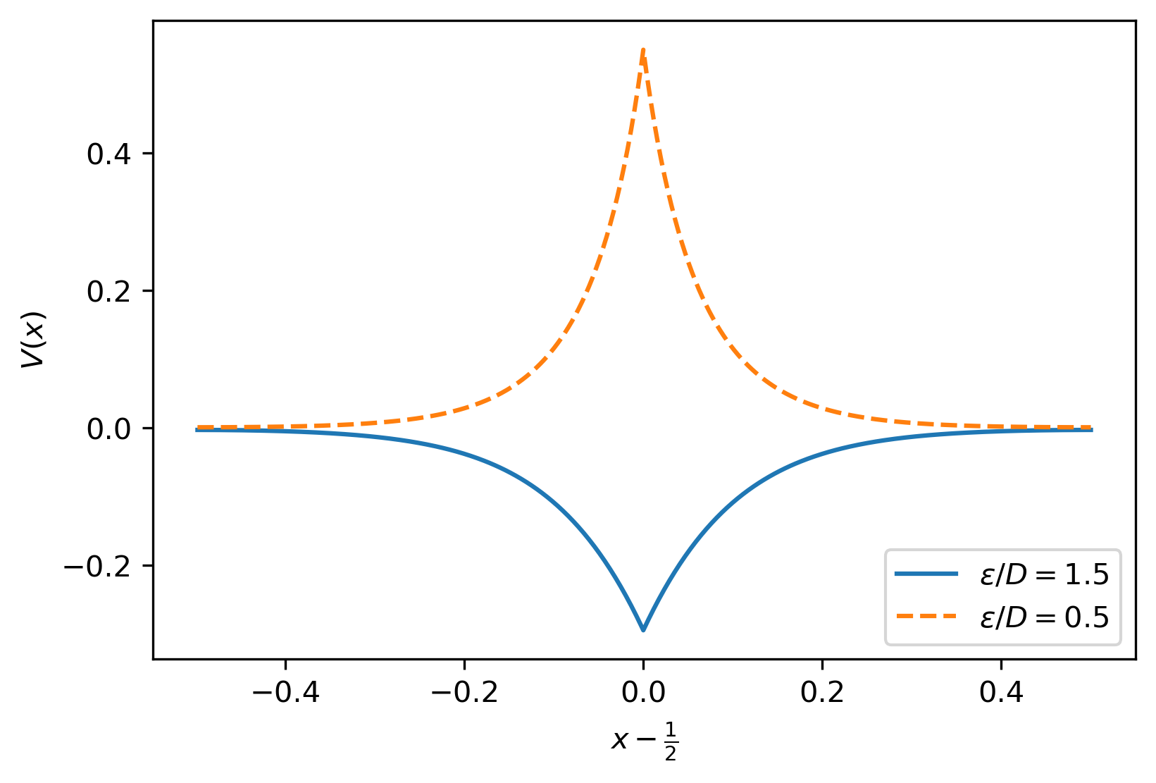
Figure 5: Comparison of the MF effective potential $V\left(x\right)$ appearing in Eq. (32) for $\varepsilon/D=1.5$ ($\varepsilon=1.5$ and $D=1$) and for $\varepsilon/D=0.5$ ($\varepsilon=1$ and $D=2$), with model parameters $\overline{\rho}=1/4$, $\overline{\tau}=1/8$, and $r=1$. These values of $\varepsilon$ and $D$ correspond to those considered in Fig. 4, showing the resetting tracers behave as an attractive potential for $\varepsilon/D=1.5$ and a repulsive potential for $\varepsilon/D=0.5$.

We conclude this section with two additional points that are worth mentioning. As found in [25], here too the resetting rate $r$ never enters the profiles in the limit $L\rightarrow\infty$. This can be heuristically understood from the fact that, in this limit, there is an infinite number of tracers in the system. Correspondingly, there is an infinite number of tracers attempting to reset their positions to the origin at any given moment. As long as the resetting attempt rate $r$ is finite (and independent of $L$), its precise value is irrelevant. Another interesting point is that, although Eqs. (13) and (14) depend on $\varepsilon$ and $D$ separately, the MF profiles depend only on the ratio $\frac{\varepsilon}{D}$ in the thermodynamic limit. It can be shown that $r$, $\varepsilon$, and $D$ do individually enter the higher order, finite-size corrections to the asymptotic profiles.

6 Conclusion and discussion

This work studies the interplay of geometric constraints and “local resetting”, where particles attempt stochastic resetting independently of one-another, thus introducing interactions into the resetting process. The dynamics associated with the classical setup of diffusive spherical particles with short-ranged repulsive interactions confined to a narrow channel is extended to include local resetting, and then its main ingredients are encoded into the dynamics of hopping particles on a $1D$ lattice ring. The lattice contains two particles species, locally resetting “tracers” of mean density $\overline{\tau}$ and non-resetting “bath” particles of mean density $\overline{\rho}$. Their continuous time evolution dynamics mimic those of the narrow channel setup: hard-core exclusion replaces the short-ranged interactions, the different masses are modeled by setting the bath and tracer diffusion rates to $1$ and $D$ respectively, and the channel’s width is replaced by a finite exchange rate $\varepsilon$. Evolution equations for the mean bath and tracer density profiles are derived, and then solved in the stationary limit using the mean-field (MF) approximation in the thermodynamic limit $L\rightarrow\infty$. The MF tracer density profile exhibits the typical tent-like shape with a cusp at the origin, as found for a single resetting diffusive particle [1]. Yet the interplay of local resetting and geometric confinement manifests most dramatically in the MF bath density profile $\rho\left(x\right)$, which transitions between “repelled” and “trapped” states as the value of $\varepsilon/D$ crosses $1$. For $\varepsilon/D<1$ bath particles are strongly repelled from the origin, with $\rho\left(x\right)$ taking the shape of an inverted tent with a negative curvature $\rho^{\prime\prime}\left(x\right)<0$. For $\varepsilon/D>1$ the bath particle are too slow to escape the dense origin and remain trapped. The shape of $\rho\left(x\right)$ is then similar to that of $\tau\left(x\right)$ and $\rho^{\prime\prime}\left(x\right)>0$. For $\varepsilon/D=1$ the bath particles experience a homogeneous environment, since hopping into a vacant site and exchanging with a tracer happen with the same rate, and we obtain $\rho\left(x\right)=\overline{\rho}$ . While the MF approximation successfully predicts the existence of both states and the transition between them, there is no a-priori reason for it to be exact in any regime. However, numerical investigations of the model provide strong evidence to suggest that the MF approximation does in fact become exact for $\varepsilon=D=1$ as $L\rightarrow\infty$. This result, whose underlying origins remain unclear, joins the observations of [25, 26] where the MF approximation was found to stand in unexpectedly good agreement with numerical simulation results of models exhibiting local resetting.

Looking forward, many interesting open questions still remain unsolved and demand attention. First and foremost, why does the MF approximation seem to work well in models featuring local resetting? Is there any way to adapt exact methods like the matrix product ansatz [51, 52], which have been used to derive exact solutions for various lattice models with exclusion interactions, to treat local resetting? Another exciting direction is to explore the temporal evolution in the presence of local resetting. While this is interesting for local resetting in general, as dynamical phase transitions were found in the temporal evolution of the density profile of a single resetting Brownian particle [9], it is even more interesting in the context of geometric confinement and tracer sub-diffusion [28, 29, 30]. In addition, both experimental and theoretical research following this line of work would of greatly benefit from pursuing a quantitative relation between the parameters describing the narrow channel setup, and the corresponding parameters of the lattice model.

7 Acknowledgments

I wish to thank David Mukamel, Oren Raz, and Shlomi Reuveni for critically reading this manuscript and for their very helpful suggestions and remarks. But, most crucially, hhis work has been made possible by the grace of DBM and the mercy of GM, to whom I am indebted to for their unconditional support.

References

- [1] Martin R. Evans and Satya N. Majumdar. Diffusion with stochastic resetting. Phys. Rev. Lett., 106:160601, Apr 2011.
- [2] Martin R Evans, Satya N Majumdar, and Kirone Mallick. Optimal diffusive search: nonequilibrium resetting versus equilibrium dynamics. Journal of Physics A: Mathematical and Theoretical, 46(18):185001, 2013.
- [3] Lukasz Kusmierz, Satya N. Majumdar, Sanjib Sabhapandit, and Grégory Schehr. First order transition for the optimal search time of lévy flights with resetting. Phys. Rev. Lett., 113:220602, Nov 2014.
- [4] Janusz M. Meylahn, Sanjib Sabhapandit, and Hugo Touchette. Large deviations for markov processes with resetting. Phys. Rev. E, 92:062148, Dec 2015.
- [5] Uttam Bhat, Caterina De Bacco, and S Redner. Stochastic search with poisson and deterministic resetting. Journal of Statistical Mechanics: Theory and Experiment, 2016(8):083401, 2016.
- [6] Arnab Pal and Shlomi Reuveni. First passage under restart. Phys. Rev. Lett., 118:030603, Jan 2017.
- [7] A. Chechkin and I. M. Sokolov. Random search with resetting: A unified renewal approach. Phys. Rev. Lett., 121:050601, Aug 2018.
- [8] Ofir Tal-Friedman, Arnab Pal, Amandeep Sekhon, Shlomi Reuveni, and Yael Roichman. Experimental realization of diffusion with stochastic resetting. The journal of physical chemistry letters, 11(17):7350–7355, 2020.
- [9] Martin R Evans, Satya N Majumdar, and Grégory Schehr. Stochastic resetting and applications. Journal of Physics A: Mathematical and Theoretical, 53(19):193001, 2020.
- [10] Andrea Montanari and Riccardo Zecchina. Optimizing searches via rare events. Phys. Rev. Lett., 88:178701, Apr 2002.
- [11] Olivier Bénichou, Claude Loverdo, Michel Moreau, and Raphael Voituriez. Intermittent search strategies. Reviews of Modern Physics, 83(1):81, 2011.
- [12] Sergey Belan. Restart could optimize the probability of success in a bernoulli trial. Phys. Rev. Lett., 120:080601, Feb 2018.
- [13] B. De Bruyne, J Randon-Furling, and S. Redner. Optimization in first-passage resetting. Phys. Rev. Lett., 125:050602, Jul 2020.
- [14] Shlomi Reuveni, Michael Urbakh, and Joseph Klafter. Role of substrate unbinding in michaelis–menten enzymatic reactions. Proceedings of the National Academy of Sciences, 111(12):4391–4396, 2014.
- [15] Tal Rotbart, Shlomi Reuveni, and Michael Urbakh. Michaelis-menten reaction scheme as a unified approach towards the optimal restart problem. Phys. Rev. E, 92:060101, Dec 2015.
- [16] Tal Robin, Shlomi Reuveni, and Michael Urbakh. Single-molecule theory of enzymatic inhibition. Nature communications, 9(1):1–9, 2018.
- [17] Iddo Eliazar, Tal Koren, and Joseph Klafter. Searching circular DNA strands. Journal of Physics: Condensed Matter, 19(6):065140, jan 2007.
- [18] Édgar Roldán, Ana Lisica, Daniel Sánchez-Taltavull, and Stephan W. Grill. Stochastic resetting in backtrack recovery by rna polymerases. Phys. Rev. E, 93:062411, Jun 2016.
- [19] Ana Lisica, Christoph Engel, Marcus Jahnel, Édgar Roldán, Eric A Galburt, Patrick Cramer, and Stephan W Grill. Mechanisms of backtrack recovery by rna polymerases i and ii. Proceedings of the National Academy of Sciences, 113(11):2946–2951, 2016.
- [20] Ricardo Falcao and Martin R Evans. Interacting brownian motion with resetting. Journal of Statistical Mechanics: Theory and Experiment, 2017(2):023204, 2017.
- [21] Martin R Evans and Satya N Majumdar. Run and tumble particle under resetting: a renewal approach. Journal of Physics A: Mathematical and Theoretical, 51(47):475003, 2018.
- [22] Anna S. Bodrova, Aleksei V. Chechkin, and Igor M. Sokolov. Scaled brownian motion with renewal resetting. Phys. Rev. E, 100:012120, Jul 2019.
- [23] Urna Basu, Anupam Kundu, and Arnab Pal. Symmetric exclusion process under stochastic resetting. Phys. Rev. E, 100:032136, Sep 2019.
- [24] S Karthika and A Nagar. Totally asymmetric simple exclusion process with resetting. Journal of Physics A: Mathematical and Theoretical, 53(11):115003, feb 2020.
- [25] Asaf Miron and Shlomi Reuveni. Diffusion with local resetting and exclusion. Phys. Rev. Research, 3:L012023, Mar 2021.
- [26] A. Pelizzola, M. Pretti, and M. Zamparo. Simple exclusion processes with local resetting. Europhysics Letters, 133(6):60003, mar 2021.
- [27] B Derrida, JL Lebowitz, and ER Speer. Large deviation of the density profile in the steady state of the open symmetric simple exclusion process. Journal of statistical physics, 107(3-4):599–634, 2002.
- [28] DW Jepsen. Dynamics of a simple many-body system of hard rods. Journal of Mathematical Physics, 6(3):405–413, 1965.
- [29] Jerome K Percus. Anomalous self-diffusion for one-dimensional hard cores. Physical Review A, 9(1):557, 1974.
- [30] S Alexander and P Pincus. Diffusion of labeled particles on one-dimensional chains. Physical Review B, 18(4):2011, 1978.
- [31] SF Burlatsky, GS Oshanin, AV Mogutov, and M Moreau. Directed walk in a one-dimensional lattice gas. Physics Letters A, 166(3-4):230–234, 1992.
- [32] SF Burlatsky, G Oshanin, M Moreau, and WP Reinhardt. Motion of a driven tracer particle in a one-dimensional symmetric lattice gas. Physical Review E, 54(4):3165, 1996.
- [33] J De Coninck, G Oshanin, and M Moreau. Dynamics of a driven probe molecule in a liquid monolayer. EPL (Europhysics Letters), 38(7):527, 1997.
- [34] C Landim, S Olla, and SB Volchan. Driven tracer particle in one dimensional symmetric simple exclusion. Communications in mathematical physics, 192(2):287–307, 1998.
- [35] O Bénichou, AM Cazabat, A Lemarchand, M Moreau, and G Oshanin. Biased diffusion in a one-dimensional adsorbed monolayer. Journal of statistical physics, 97(1-2):351–371, 1999.
- [36] Raphaël Candelier and Olivier Dauchot. Journey of an intruder through the fluidization and jamming transitions of a dense granular media. Physical Review E, 81(1):011304, 2010.
- [37] P Illien, O Bénichou, C Mejía-Monasterio, G Oshanin, and R Voituriez. Active transport in dense diffusive single-file systems. Physical review letters, 111(3):038102, 2013.
- [38] J Cividini, A Kundu, Satya N Majumdar, and D Mukamel. Correlation and fluctuation in a random average process on an infinite line with a driven tracer. Journal of Statistical Mechanics: Theory and Experiment, 2016(5):053212, 2016.
- [39] Julien Cividini, Anupam Kundu, Satya N Majumdar, and David Mukamel. Exact gap statistics for the random average process on a ring with a tracer. Journal of Physics A: Mathematical and Theoretical, 49(8):085002, 2016.
- [40] A Kundu and J Cividini. Exact correlations in a single-file system with a driven tracer. EPL (Europhysics Letters), 115(5):54003, 2016.
- [41] Julien Cividini, David Mukamel, and HA Posch. Driven tracers in narrow channels. Physical Review E, 95(1):012110, 2017.
- [42] Sheida Ahmadi and Richard K Bowles. Diffusion in quasi-one-dimensional channels: A small system n, p, t, transition state theory for hopping times. The Journal of chemical physics, 146(15):154505, 2017.
- [43] Olivier Bénichou, Vincent Démery, and Alexis Poncet. Unbinding transition of probes in single-file systems. Physical review letters, 120(7):070601, 2018.
- [44] Asaf Miron, David Mukamel, and Harald A Posch. Phase transition in a 1d driven tracer model. Journal of Statistical Mechanics: Theory and Experiment, 2020(6):063216, jun 2020.
- [45] Asaf Miron and David Mukamel. Driven tracer dynamics in a one dimensional quiescent bath. Journal of Physics A: Mathematical and Theoretical, 54(2):025001, dec 2020.
- [46] Asaf Miron, David Mukamel, and Harald A. Posch. Attraction and condensation of driven tracers in a narrow channel. Phys. Rev. E, 104:024123, Aug 2021.
- [47] Gunter Schütz and Eytan Domany. Phase transitions in an exactly soluble one-dimensional exclusion process. Journal of statistical physics, 72(1):277–296, 1993.
- [48] Gunter M Schütz. Exact solution of the master equation for the asymmetric exclusion process. Journal of statistical physics, 88(1):427–445, 1997.
- [49] Bernard Derrida. An exactly soluble non-equilibrium system: the asymmetric simple exclusion process. Physics Reports, 301(1-3):65–83, 1998.
- [50] J Cividini, D Mukamel, and HA Posch. Driven tracer with absolute negative mobility. Journal of Physics A: Mathematical and Theoretical, 51(8):085001, 2018.
- [51] Richard A Blythe and Martin R Evans. Nonequilibrium steady states of matrix-product form: a solver’s guide. Journal of Physics A: Mathematical and Theoretical, 40(46):R333, 2007.
- [52] Thomas Kriecherbauer and Joachim Krug. A pedestrian’s view on interacting particle systems, kpz universality and random matrices. Journal of Physics A: Mathematical and Theoretical, 43(40):403001, 2010.