Fine-grained Few-shot Recognition by Deep Object Parsing

Abstract

We propose a new method for fine-grained few-shot recognition via deep object parsing. In our framework, an object is made up of $K$ distinct parts and for each part, we learn a dictionary of templates, which is shared across all instances and categories. An object is parsed by estimating the locations of these $K$ parts and a set of active templates that can reconstruct the part features. We recognize test instances by comparing its active templates and the relative geometry of its part locations against those of the presented few-shot instances. Our method is end-to-end trainable to learn part templates on-top of a convolutional backbone. To combat visual distortions such as orientation, pose and size, we learn templates at multiple scales, and at test-time parse and match instances across these scales. We show that our method is competitive with the state-of-the-art, and by virtue of parsing enjoys interpretability as well.

1 Introduction

Deep neural networks (DNN) can be trained to solve visual recognition tasks with large annotated datasets. In contrast, training DNNs for few-shot recognition Snell et al. (2017); Vinyals et al. (2016), and its fine-grained variant Sun et al. (2020), where only a few examples are provided for each class by way of supervision at test-time, is challenging.

Fundamentally, the issue is that few-shots of data is often inadequate to learn an object model among all of its myriad of variations, which do not impact an object’s category.

For our solution, we propose to draw upon two key observations from the literature.

• There are specific locations bearing distinctive patterns/signatures in the feature space of a convolution neural network (CNN), which correspond to salient visual characteristics of an image instance Zhou et al. (2014); Bau et al. (2017).

• Attention on only a few specific locations in the feature space, leads to good recognition accuracy Zhu et al. (2020); Lifchitz et al. (2021); Tang et al. (2020).

How can we leverage these observations?
Duplication of Traits. We posit that the visual characteristics found in one instance of an object are widely duplicated among other instances, and even among those belonging to other classes. It follows from our proposition that it is the particular collection of visual characteristics arranged in a specific geometric pattern that uniquely determines an object belonging to a particular class.

These assumptions, along with (A) and (B), imply that these shared visual traits can be found in the feature maps of CNNs and only a few locations on the feature map suffice for object recognition. CNN features are important, as they distill essential information, and suppress redundant or noisy information.

Parsing. We call these finitely many latent locations on the feature maps which correspond to salient traits, parts. These parts manifest as patterns, where each pattern belongs to a finite (but potentially large) dictionary of templates. This dictionary embodies both the shared vocabulary and the diversity of patterns found across object instances. Our goal is to learn the dictionary of templates for different parts using training data, and at test-time, we seek to parse new instances by identifying part locations and the sub-collection of templates that are expressed for the few-shot task. The provided few-shot instances are parsed and then compared against the parsed query. The best matching class is then predicted as the output. As an example see Fig 1 (a), where the recognized part locations using the learned dictionary correspond to the head, breast and the knee of the birds in their images with corresponding locations in the convolutional feature maps. In matching the images, both the constituent templates and the geometric structure of the parts are utilized.

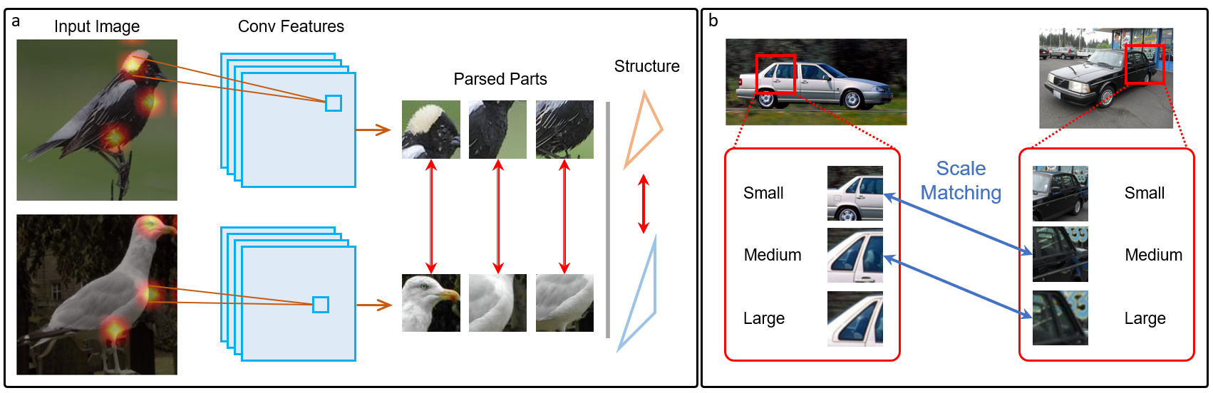
Figure 1: Motivation: a) In fine-grained few-shot learning, the most discriminating information is embedded in the salient parts (e.g. head and breast of a bird) and the geometry of the parts (relative part locations). Our method parses the object into a structured combination of a finite set of dictionaries, such that both finer details and the shape of the object are captured and used in recognition. b) In few shot learning, the same part may be distorted or absent in the support samples due to the perspective and pose changes. We propose to extract features and compare across multiple scales for each part to overcome this.

Inferring part locations based on part-specific dictionaries is a low complexity task, and is analogous to the problem of detection of signals in noise in radar applications Van Trees (2004), a problem solved by matching the received signal against a known dictionary of transmitted signals.

Challenges. Nevertheless, our situation is somewhat more challenging. Unlike the radar situation, we do not a-priori have a dictionary, and to learn one, we are only provided class-level annotations by way of supervision. In addition, we require that these learnt dictionaries are compact (because we must be able to reliably parse any input), and yet sufficiently expressive to account for diversity of visual traits found in different objects and classes.

Multi-Scale Dictionaries. Variation in pose and orientation lead to different appearances by perspective projections, which means there is variation in the scale and size of visual characteristics of parts. To overcome this issue we train dictionaries at multiple scales, which leads us to a parsing scheme that parses input instances at multiple scales (see Fig. 1 (b)).

Goodness of fit. Besides part sizes, few-shot instances even within the same class may exhibit significant variations in poses, which can in-turn induce variations in parsed outputs. To mitigate their effects we propose a novel instance-dependent re-weighting method, for comparison, based on goodness-of-fit to the dictionary.

Contributions. We show that: (i) Our deep object parsing method, results in improved performance in few-shot recognition and fine-grained few-shot recognition tasks on Stanford-Car dataset outperforming prior art by 2.64%. (ii) We provide an analysis of different components of our approach showing the effect of ablating each in final performance. Through a visualization, we show that the parts recognized by our model are salient and help recognize the object category.

2 Related Work

Few-Shot Classification (FSC). Modern FSC methods can be classified into three categories: metric-learning based, optimization-based, or data-augmentation methods. Methods in the first category focus on learning effective metrics to match query examples to support. Prototypical Network Snell et al. (2017) utilizes euclidean distance on feature space for this purpose. Subsequent approaches built on this by improving the image embedding space Ye et al. (2020); Das et al. (2021); Afrasiyabi et al. (2021); Zhou et al. (2021); Rizve et al. (2021) or focusing on the metric Sung et al. (2018); Wang et al. (2019); Bateni et al. (2020); Simon et al. (2020); Li et al. (2020a); Wertheimer et al. (2021); Fei et al. (2021); Zhang et al. (2020; 2021). Some recent methods have also found use of graph based methods, especially in transductive few shot classification Chen et al. (2021); Yang et al. (2020). Optimization based methods train for fast adaptation using a few parameter updates with the support examples Finn et al. (2017); Baik et al. (2021); Li et al. (2017); Lee et al. (2019); Rajeswaran et al. (2019); Liu et al. (2018). Data-augmentation methods learn a generative model to synthesize additional training data for the novel classes to alleviate the issue of insufficient data Li et al. (2020b); Schwartz et al. (2018); Wang et al. (2018); Xu et al. (2021).

Fine-grained FSC. In fine-grained few-shot classification, different classes differ only in finer visual details. An example of this is to tease apart different species of birds in images. The approaches mentioned above have been applied in this context as well Li et al. (2019); Sun et al. (2020); Li et al. (2020c); Xu et al. (2021). Li et al. (2019) proposes to learn a local descriptor and an image-to-class measure to capture the similarity between objects. Wang et al. (2021) uses a foreground object extractor to exclude the noise from background and synthesize foreground features to remedy the data insufficiency. BSNet Li et al. (2020c) leverages a bi-similarity module to learn feature maps of diverse characteristics to improve the model’s generalization ability. Variational feature disentangling (VFD) Xu et al. (2021), a data-augmentation method, is complementary to ours. It disentangles the feature representation into intra-class variance and class-discriminating information to emphasize the inter-class differences, and generates additional features for novel classes to mitigate data scarcity at test-time. TDMLee et al. (2022) applies channel-wise attention to represent different classes with sparse vectors while we decompose a object into meaningful parts with vectors.

In addition, prior works on attention has been found to be effective both in few-shot learning and its fine-grained version. This approach seeks to extract most discriminative image features and ignore background information irrelevant to object class Jiang et al. (2020); Zhu et al. (2020); Lifchitz et al. (2021); Kang et al. (2021). In related work, Cao et al. (2020) propose training fixed masks on feature space, and leveraging outputs from each mask for FSC.

Recognition using Object Parts. Our method is closely related to recognition based on identifying object components, an approach motivated by how humans learn to recognize object Biederman (1987). It draws inspiration from Ullman et al. (2002), who showed that information maximization with respect to classes of images resulted in visual features eyes, mouth, etc. in facial images and tyres, bumper, windows, etc. in images of cars. Along these lines, Deformable Part Models (DPM) Felzenszwalb et al. (2009; 2010) proposed to learn object models by composing part features and geometries, and utilize it for object detection. Neural Network models for DPMs were proposed in Savalle et al. (2014); Girshick et al. (2015). Multi-attention based models, which can be viewed as implicitly incorporating parts, have been proposed Zheng et al. (2017) in the context of fine-grained recognition problems. Although related, a principle difference is our few-shot setting, where new classes emerge, and we need to generate new object models on-the-fly.

Prior works on FSC have also focused on combining parts, albeit with different notions of the concept. As such, the term part is overloaded, and is unrelated to our notion. DeepEMD Zhang et al. (2020) focuses in the image-distance metric based on an earth mover’s distance between different parts. Here, parts are simply different physical locations in the image and not a compact collection of salient parts for recognition. Tang et al. (2020) uses salient object parts for recognition, while Tokmakov et al. (2019) attempts to encode parts into image features. However, both these methods require additional attribute annotations for training, which may be expensive to gather and not always available. Hao et al. (2019) and Wu et al. (2021) discover salient object parts and use them for recognition via attention maps similar to our method. They also re-weigh their similarity task-adaptively, which is also a feature of our method. We differ in our use of a finite dictionary of templates used to learn a compact representation of parts. Also, we use reconstruction as supervision for accurately localizing salient object parts, and impose a meaningful prior on the geometry of parts, which keeps us from degenerate solutions for part locations.

3 Deep Object Parsing

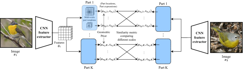
Figure 2: Deep Object Parsing. An image is parsed as a collection of salient parts. Each part is represented by a 2D location and part expression vector. In our method, we estimate locations and expressions at multiple scales for each part and using these, determine image similarity for few-shot recognition. (Best viewed with zoom)

Input instances are denoted by $x\in{\cal X}$ and we denote by $\phi\in\mathbb{R}^{G\times G\times C}$ the output features of a CNN, with $C$ channels, supported on a 2D, $G\times G$, grid.
Parsing Instances. A parsed instance has $K$ distinct parts. While this term, “parts”, is overloaded in prior works, our notion of a part is a tuple, consisting of part-location and part-expression at that location. The location corresponds to an $s\times s$ attention mask, $M(\mu)$ centered around the location $\mu\in[G]\times[G]$ in the CNN feature space.

Also integral to our parsing are a set of learned templates in feature space ${D}_{p,c}\in\mathbb{R}^{s\times s},p\in[K],c\in[C]$. Given these templates, part-expressions are a set of reconstruction coefficients $z_{p,c}(\mu)\in\mathbb{R},p\in[K],c\in[C]$ such that we reconstruct features as $\phi_{c,M_{\mu_{p}}}\approx z_{p,c}D_{p,c}$, where the subscript $M_{\mu_{p}}$ denotes a projection onto its support. We assume that the part templates are exhaustive across input categories. Once parsed, each instance is represented using its part locations $\mu_{p}\in[G]\times[G]$ and expressions $z_{p}\in\mathbb{R}^{C}$ for each $p\in[K]$.

Part Expression as LASSO Regression. Given an instance $x$, its feature output, $\phi$, and a candidate part-location, $\mu$, we can estimate sparse part-expression coefficients $z_{p}(\mu)\in\mathbb{R}^{C}$ by optimizing the $\ell_{1}$ regularized reconstruction error, at the location $\mu=\mu_{p}$.

$$z_{p}(\mu)=\arg\min_{\beta}\sum_{c\in C}\|\phi_{c,M(\mu)}-D_{p,c}\beta_{c}\|^{2}+\lambda\|\beta\|_{1}.$$ (1)

Non-negativity. Part expressions $z_{p,c}$ signify presence or absence of part templates in the observed feature vectors, and as such can be expected to take on non-negative values. This fact turns out to be useful later for DNN implementation.

Part Location Estimation. Note that part expression $z_{p}$ is a function of location $\mu$, while the part location $\mu_{p}$ can be estimated by plugging in the optimal part-expressions for each candidate location value, namely,

$$\mu_{p}=\operatorname*{arg\,min}_{\mu\in[G]\times[G]}\sum_{c\in C}\|[\phi_{c}]_{M(\mu)}-D_{p,c}z_{p,c}(\mu)\|^{2}+\lambda\|z_{p}(\mu)\|_{1}$$ (2)

This couples the two estimation problems, and is difficult to implement with DNNs, motivating our approach below.

Feedforward DNNs for Parsing. To make the proposed approach amenable to DNN implementation, we approximate the solution to Eq. 1 by optimizing the reconstruction error followed by thresholding, namely, we compute $z_{p}^{\prime}(\mu)=\arg\min_{\beta}\sum_{c\in C}\|\phi_{c,M(\mu)}-D_{p,c}\beta_{c}\|^{2}$, and we threshold the resulting output by deleting entries smaller than $\zeta$: $S_{\zeta}(u)=u\mathbf{1}_{|u|\geq\zeta}$. This is closely related to thresholding methods employed in LASSO Hastie et al. (2001).

The quadratic component of the loss allows for an explicit solution, and the solution reduces to template matching per channel, which can further be expressed as a convolution Gonzalez & Woods (2008). Using this insight, we derive our estimate of $\mu_{p}$ as

$$\mu_{p}=\operatorname*{arg\,max}_{\mu\in[G]\times[G]}\sum\limits_{c\in C}((\theta_{p,c}\ast\phi_{c})(\mu)-\lambda_{c})^{2}$$ (3)

where $\theta_{p,c}=D_{p,c}/\|D_{p,c}\|$, and $\lambda_{c}=\lambda/2\|D_{p,c}\|$ becomes a channel dependent constant. With the above estimate of $\mu_{p}$, we get the estimate of $z_{p}$ as:

$$z_{p,c}^{\prime}=\frac{(D_{p,c}\ast\phi_{c})(\mu_{p})}{\|D_{p,c}\|^{2}};\,\,\,z_{p,c}(\mu)=S_{\zeta}(z_{p,c}^{\prime})$$ (4)

where ‘$:$’ is the double dot product—sum over all entries of the element-wise (Hadamard) product and $z_{p,c}$ is the $c^{th}$ element of $z_{p}$. For a full derivation of the above estimates, please refer to the supplementary materials (App. A).

Estimates differentiable in parameters. Since argmax is a non-differentiable function, using Eq. 3 for estimating part-locations does not allow us to use gradient based learning for the parameters of the DNN. We can circumvent this by approximating the argmax as the expectation of a softmax distribution $\nu_{p}$ over $[G]\times[G]$ with a low temperature $T$.

$$\nu_{p}(\mu)=\text{softmax}\left(\frac{1}{T}\sum\limits_{c\in C}((\theta_{p,c}\ast\phi_{c})(\mu)-\lambda_{c})^{2}\right);\quad\mu_{p}=\mathbb{E}_{\mu\sim\nu_{p}}\mu$$ (5)

Similarly, we get a differentiable estimate of part expressions as

$$z_{p,c}^{\prime}=\mathbb{E}_{\mu\sim\nu_{p}}\left[\frac{(D_{p,c}\ast\phi_{c})(\mu)}{\|D_{p,c}\|^{2}}\right];\,\,\,z_{p,c}=S_{\zeta}(z_{p,c}^{\prime})$$ (6)

Multi-Scale Extension. We extend our approach to incorporate parsing parts at multiple scales. This is often required because of significant difference in orientation and pose between query and support examples. To do so we simply consider masks $M(\mu)$ and templates $D$ at varying mask sizes $s\in{\mathcal{S}}$, each leading to independent part location and expression estimates ($\mu_{s,p}$, $z_{s,p}$) for part $p$. Alg. 1 specifies the parse of an input instance and Fig. 2 shows an overview of object parsing.

1 Given: Convolutional backbone $f$, templates $\{D_{s,p,c}\}_{s\in{\mathcal{S}},p\in[K],c\in[C]}$, threshold $\zeta$, $\ell_{1}$ regularization constant $\lambda$, temperature $T$

2 Input: Image $x$

3 Compute convolutional features $\phi=f(x)$

4 for $p\in[K],s\in{\mathcal{S}}$ do

5       Estimate $\mu_{s,p}$ (through $\nu_{s,p}$) using Eq. 5

6       Estimate $z_{s,p}=[z_{s,p,c}]_{c\in[C]}$ using Eq. 6

7 end for

8

Output: Part locations and expressions ($\{\mu_{s,p}\}_{p\in[K],s\in{\mathcal{S}}}$, $\{z_{s,p}\}_{p\in[K],s\in{\mathcal{S}}}$)

Algorithm 1 PARSE (Object Parsing using DNNs)

3.1 Few-Shot Recognition

At test-time we are given a query instance, $q$, and by way of supervision, $M$ support examples each for $N$ classes, and the goal is to predict the query class label $y^{(q)}\in[N]$. We first run PARSE (Alg. 1) on each of these. $\texttt{PARSE}(q)=(\{\mu_{s,p}^{(q)}\},\{z_{s,p}^{(q)})\}$ and for the $i^{th}$ support example of class $y$, $\texttt{PARSE}(x^{(i,y)})=(\{\mu_{s,p}^{(i,y)}\},\{z_{s,p}^{(i,y)}\})$. For comparing query and support examples we need a notion of distance/similarity, which we define next.

Goodness-of-fit reweighting. The entropy of the distribution $\nu_{s,p}$ is an important indicator of goodness-of-fit of the dictionary templates (lower entropy meaning a more precise and confident part-location prediction as a result of a better fit). Let $h_{s,p}^{(q)}$ and $h_{s,p}^{(i,y)}$ be the entropies of $\nu_{s,p}^{(q)}$ and $\nu_{s,p}^{(i,y)}$ respectively. To use these as weights for computing distance (as below), we learn a simple parametric function $\alpha:\mathbb{R}^{M+1}\rightarrow\mathbb{R}$.

Additionally, with $z_{s,p}^{(y)}=\sum_{i\in[M]}z_{s,p}^{(i,y)},s\in{\mathcal{S}},p\in[K]$ we represent the mean part expression over all support examples in class $y$. With these, we define the following distance measure between the query example $q$ and the support examples of class $y$.

$$d(q,y)= \sum_{p\in[K]}\sum_{s_{1}\in{\mathcal{S}}}\sum_{s_{2}\in{\mathcal{S}}}\alpha(h_{s_{1},p}^{(q)},[h_{s_{2},p}^{(i,y)}]_{i\in[M]})\left\|z_{s_{1},p}^{(y)}-z_{s_{2},p}^{(q)}\right\|^{2}\quad\text{[expression distance]}$$

$$+\gamma\sum_{i\in[M]}\sum_{s_{1}\in{\mathcal{S}}}\sum_{s_{2}\in{\mathcal{S}}}\left\|\psi([\mu_{s_{1},p}^{(i,y)}]_{p\in[K]})-\psi([\mu_{s_{2},p}^{(q)}]_{p\in[K]})\right\|^{2}\quad\text{[geometric distance]}$$ (7)

where $\psi([\mu_{s,p}]_{p\in[K]})$ is a vector of pairwise distances between all part locations at scale $s$, normalized to unit sum. The distance function consists of an expression term, and a geometric term with $\gamma$ acting as a tunable weight to control the proportion of the two. Each term is a sum over all combinations of part scales over query and support. Note that the geometric term simply attempts to find if two polygons with vertices at part locations are similar (i.e. have proportional sides), with the distance being $0$ if they are. Finally, the class prediction is made as $\widehat{y}^{(q)}=\operatorname*{arg\,min}_{y\in[N]}d(q,y)$.

Training. We train in episodes following convention. For each episode, we sample $N$ classes at random, and additionally sample support and query examples belonging to these classes from training data (details in Sec. 4). Using a softmax over the negative distance function above as the class distribution of query $q$, we define the cross-entropy loss as

$$\ell_{CE}(q)=-\log\frac{\exp(-d(q,y^{(q)}))}{\sum_{y\in[N]}\exp(-d(q,y))}$$ (8)

Additionally, while training, we impose a geometric prior to get diverse instance parts in PARSE by maximizing the Hellinger distance Everitt (1998) $\mathbb{H}(\cdot,\cdot)$ between part distributions. The corresponding criterion for minimization is

$$\ell_{div}(x)=-\sum_{s\in{\mathcal{S}}}\sum_{\begin{subarray}{c}p,p^{\prime}\in[K]\\ p\neq p^{\prime}\end{subarray}}\mathbb{H}(\nu_{s,p},\nu_{s,p^{\prime}})$$ (9)

Alg. 2 outlines the loss computation for a single query $q$. In Alg. 2, $\eta$ is a tunable parameter controlling the weight of the prior. In each episode, we use an average of the loss output over multiple query examples, which results in an end-to-end differentiable criterion in all trainable parameters, allowing us to optimize using gradient descent.

1 Given: requirements for Alg. 1 PARSE, weighting function $\alpha$, tunable parameter $\gamma$

2 Input: Query example with ground truth label $q,y^{(q)}\in{\mathcal{X}}\times[N]$. Support examples $I=\bigcup_{y\in[N]}\left[I_{y}=\{x^{(i,y)}\}_{i\in[M]}\right]$

3 Trainable parameters: Convolutional backbone $f$, part templates $\{D_{s,p,c}\}_{s\in{\mathcal{S}},p\in[K],c\in[C]}$, weighting function $\alpha$

4

5Compute parses $\texttt{PARSE}(q)=(\{\mu_{s,p}^{(q)}\},\{z_{s,p}^{(q)})\}$, $\texttt{PARSE}(x^{(i,y)})=(\{\mu_{s,p}^{(i,y)}\},\{z_{s,p}^{(i,y)}\});s\in{\mathcal{S}},p\in[K]$

6 Compute distances $d(q,y)$ for $y\in[N]$ using Sec. 3.1

7 Output: loss $\ell(q)=\ell_{CE}(q)+\eta\frac{1}{|I|+1}\sum_{x\in I\cup\{q\}}\ell_{div}(x)$ using Eqs. 8, LABEL: and 9

Algorithm 2 Training loss for Few-shot recognition with DOP (single episode, single query)

3.2 Implementation Details

We use two Resnet He et al. (2016) backbones (Resnet-12 and Resnet-18) as feature extractors. We use the Resnet-12 model used in prior works Lee et al. (2019), which has more output channels and more parameters (12.4M) compared to Resnet-18 (11.2M). The input image is resized to 84 $\times$ 84 for Resnet-12 and 224 $\times$ 224 for Resnet-18. In the output features, for Resnet-12, $C=640$ and $G=5$, and for Resnet-18, $C=512$ and $G=7$.

The number of parts $K$ is set to 4 for most experiments (see Sec. 4.2 for a experiments with different number of parts).

There are three scales ${\mathcal{S}}=\{1,3,5\}$ considered for each part. The temperature $T$ in Eq. 5 is set to $0.01$ and the threshold $\zeta$ in Eq. 6 is set to $0.05$. $\gamma$ is set to 0.01. For $\alpha$ we used a linear layer, and subsequently normalized $[\alpha(h_{s_{1},p}^{(q)},[h_{s_{2},p}^{(i,y)}]_{i\in[M]})]_{p\in[K]}$(a K-dimensional vector; see Sec. 3.1) with a softmax.

4 Experiments

4.1 Fine-grained Few-Shot Classification

We compare DOP on four fine-grained datasets: Caltech-UCSD-Birds (CUB) Wah et al. (2011), Stanford-Dog (Dog) Khosla et al. (2011) Stanford-Car (Car) Krause et al. (2013) and Aircraft Maji et al. (2013) against state-of-the-art methods.

Caltech-UCSD-Birds (CUB) Wah et al. (2011) is a fine-grained classification dataset with 11,788 images of 200 bird species. Following conventionHilliard et al. (2018), the 200 classes are randomly split into 100 base, 50 validation and 50 test classes.

Aircraft contains 100 classes of aircrafts and 10,000 images in total. Following recent benchmark Lee et al. (2022) Wertheimer et al. (2021), we processes all images based on bounding box. And the 100 classes are split into 50, 25 and 25 classes for training, validation and test.

Stanford-Dog/Car Khosla et al. (2011); Krause et al. (2013) are two datasets for fine-grained classification. Dog contains 120 dog breeds with a total number of 20,580 images, while Car consists of 16,185 images from 196 different car models. For few-shot learning evaluation, we follow the benchmark protocol proposed in Li et al. (2019). Specifically, 120 classes of Dog are split into 70, 20, and 30 classes, for training, validation, and test, respectively. Similarly, Car is split into 130 train, 17 validation and 49 test classes.

Experiments Setup. We conducted 5-way (5 classes episode) 1-shot and 5-way 5-shot classification tasks on all datasets. Following the episodic evaluation protocol in Vinyals et al. (2016), at test time, we sample 600 episodes and report the averaged Top-1 accuracy. In each episode, 5 classes from the test set are randomly selected. 1 or 5 samples for each class are sampled as support data, and another 15 examples are sampled for each class as the query data. The model is trained on train split and the validation split is used to select the hyper-parameters. We compare our DOP to state-of-the-art few-shot learning methods Kang et al. (2021); Wertheimer et al. (2021); Lee et al. (2022); Zhang et al. (2020) and fine-grained few shot learning methods: FOTWang et al. (2021), VFD Xu et al. (2021), DN4Li et al. (2019) and TDMLee et al. (2022). More details on these methods are in the supplementary (App. B).

Training Details. Our model is trained with 10,000 episodes on CUB and 30,000 episodes on Stanford-Dog/Car for experiments with both ResNet12 and ResNet18. In each episode, we randomly select 10 classes and sample 5 and 10 samples as support and query data. The weight on the geometric prior $\eta$ is set to 1.0 on CUB and 0.1 on Stanford-Dog/Car, respectively.

We train from scratch with Adam optimizer Kingma & Ba (2014). The learning rate starts from 5e-4 on CUB and 1e-3 on Stanford-Car/Dog, and decays to 0.1x every 3,000 episodes on CUB and 9,000 episodes on Dog/Car. On CUB, objects are cropped using the annotated bounding box before resizing to the input size. On Stanford-Car/Dog, we use the resized raw image as the input. We employed standard data augmentations, including horizontal flip and perspective distortion, to the input images.

Table 1: Few-shot accuracy in $\%$ on CUB (along with 95% confidence intervals). If not specified, the results is reported by the original paper. *: results reported in Xu et al. (2021). $\dagger$: results are obtained by running the public implementations released by authors using ResNet18 backbone.

Methods	Backbone	1-shot	5-shot
ProtoNetSnell et al. (2017)	ResNet18	71.88$\pm$0.91	87.42$\pm$0.48
Baseline++Chen et al. (2019)	ResNet18	67.02$\pm$0.9	83.58$\pm$0.54
SimpleShotWang et al. (2019)	ResNet18	62.85$\pm$0.20	84.01$\pm$0.14
DN4Li et al. (2019)$\dagger$	ResNet18	70.47$\pm$0.72	84.43$\pm$0.45
AFHNLi et al. (2020b)	ResNet18	70.53$\pm$1.01	83.95$\pm$0.63
$\Delta$-encoderSchwartz et al. (2018)	ResNet18	69.80$\pm$0.46	82.60$\pm$0.35
BSNetLi et al. (2020c)	ResNet18	69.61$\pm$0.92	83.24$\pm$0.60
FOTWang et al. (2021)	ResNet18	72.56$\pm$0.77	87.22$\pm$0.46
MTLLiu et al. (2018)*	ResNet12	73.31 $\pm$ 0.92	82.29 $\pm$0.51
MetaOptNetLee et al. (2019)*	ResNet12	75.15$\pm$0.46	87.09$\pm$0.30
DeepEMDZhang et al. (2020)	ResNet12	75.65$\pm$0.83	88.69$\pm$0.50
VFD Xu et al. (2021)	ResNet12	79.12$\pm$0.83	91.48$\pm$0.39
FRNWertheimer et al. (2021)	ResNet12	83.16	92.59
RENetKang et al. (2021)	ResNet12	79.49$\pm$0.44	91.11$\pm$0.24
TDMLee et al. (2022)	ResNet12	83.36	92.80
DOP	ResNet18	82.62$\pm$0.65	92.61$\pm$0.38
DOP	ResNet12	83.39$\pm$0.82	93.01$\pm$0.43

Table 2: Few-shot classification accuracy in % on Aircraft dataset. Unless specified, methods use ResNet-12 backbone.

Methods	1-shot	5-shot
ProtoNetSnell et al. (2017)	67.28	83.21
DSNSimon et al. (2020)	70.23	83.03
CTXDoersch et al. (2020)	71.57	79.31
FRNWertheimer et al. (2021)	69.58	83.98
TDMLee et al. (2022)	71.57	84.77
DOP (ResNet18)	84.26	93.41
DOP (ResNet12)	85.50	94.35

Results. Our results along with comparisons against state-of-the-art on CUB, Aircraft and Stanford-Dog/Car are reported in Tabs. 1, LABEL:, 2, LABEL: and 3, respectively.

DOP  is competitive with or outperforms recent works on fine-grained FSC. On CUB (Tab. 1), DOP outperforms all compared approaches with 83.39% 1-shot accuracy and 93.01% for 5-shot with Resnet-12 backbone. Same is the case for Aircraft (Tab. 2), where DOP outperforms a recent method in TDM Lee et al. (2022) by a large margin using ResNet-12 backbone, performing at 85.50% 1-shot and 94.35% 5-shot accuracy. While on Stanford-Car (Tab. 3), we outperform compared approaches by 3.06% and 1.85% on 1-shot and 5-shot, respectively, on Stanford-Dog, we outperform all methods but VFD. We note here that VFD generates additional features at test-time for novel classes, and is as such, complementary to DOP .

Table 3: Few-shot classification accuracy in % on Stanford-Car/Dog benchmarks (along with 95% confidence intervals). *: results reported in Xu et al. (2021). $\dagger$: results are obtained by running the codes released by authors using ResNet18 backbone.

Methods	Backbones	Car		Dog
		1-shot	5-shot	1-shot	5-shot
ProtoNet$\dagger$Snell et al. (2017)	ResNet18	60.67$\pm$0.87	75.56$\pm$0.45	61.06$\pm$0.67	74.31$\pm$0.51
DN4$\dagger$Li et al. (2019)	ResNet18	78.77$\pm$0.81	91.99$\pm$0.41	60.73$\pm$0.67	75.33$\pm$0.38
MetaOptNet$\dagger$Lee et al. (2019)	ResNet18	60.56$\pm$0.78	76.35$\pm$0.52	65.48$\pm$0.56	79.39$\pm$0.43
MTL*Liu et al. (2018)	ResNet12	-	-	54.96$\pm$1.03	68.76$\pm$0.65
$\Delta$-encoder*Schwartz et al. (2018)	ResNet12	-	-	68.59$\pm$0.53	78.60$\pm$0.78
BSNetLi et al. (2020c)	ResNet12	60.36$\pm$0.98	85.28$\pm$0.64	69.09$\pm$0.90	82.45$\pm$0.58
VFD*Xu et al. (2021)	ResNet12	-	-	76.24$\pm$0.87	88.00$\pm$0.47
DOP	ResNet18	81.41$\pm$ 0.71	93.48$\pm$ 0.38	70.56$\pm$ 0.75	84.75$\pm$ 0.41
DOP	ResNet12	81.83$\pm$ 0.78	93.84$\pm$ 0.45	70.10$\pm$ 0.79	85.12$\pm$ 0.55

4.2 Analyses

We conducted a series of analyses to study the effects of different components of DOP  on fine-grained datasets based on 5-shot accuracy with the Resnet-18 backbone.

Instance-dependent reweighting based on goodness-of-fit. We use a parametric reweighting function $\alpha$ that reweights the distances between part expressions based on the how well the learned templates fit the part features (see Sec. 3.1). In Tab. 4, we show the effect of removing this reweighting, and simply using an average of all pairs of distances between the query and support. As we see the reweighting function does help FSL accuracy.

Effect of using part-geometry for comparison. In Sec. 3.1, we use part geometries besides part expressions for computing distances. Tab. 4 also shows scenarios where we remove this component in the distance (equivalent to setting $\gamma=0$). We see that using a distance between part geometries help final FSL performance.

Table 4: 5-way 5-shot accuracy on ablating components in distance computation: re-weighting function $\alpha$ and using part-geometry (Sec. 3.1). Both components help FSL accuracy independently as well as together.

Part-geometry	Re-weighting	CUB	Dog	Car
		91.83	82.07	92.78
	✓	92.44	83.90	93.31
✓		91.95	83.33	93.21
✓	✓	92.61	84.75	93.48

Effect of using templates at multiple scales. In Tab. 6 we ablated different choices of scales on Dog. Using multiple scales is better than a single scale, and using all the scales obtains the best performance. This validates our hypothesis that parts are distorted due to pose variations, and a single scale is not sufficient to represent the object in a few-shot scenario.

Effect of using different number of parts. Tab. 6 shows the effect of using different number of parts on 5-way 5-shot accuracy on CUB. $K=4$ has the best accuracy and performance drops with more parts as the model starts learning irrelevant or background signatures.

Table 5: Effect of using templates at different scales on 5-way 5-shot classification accuracy on Dog.

Scales	[3]	[5]	[3,5]	[1,3,5]
Accuracy	81.56	81.38	83.04	84.75

Table 6: Effect of using different number of parts on 5-way 5-shot classification accuracy on CUB.

Num parts	3	4	5	6
Accuracy	92.10	92.61	92.21	92.06

What parts does DOP detect? We visualize the locations $\mu_{p}$ learned by DOP in Fig. 3. DOP is able to detect consistent parts for the same task and often finds semantically meaningful parts like head and torso/breast in birds and dogs and wheels and doors/windows on cars. Fig. 3 also shows some failure cases of DOP , where it might fail to locate parts on the object if similar visual signatures appear in the background. A visualization of part templates learned and part expressions can be found in the supplementary (App C).

Figure 3: Exemplar part locations learned by DOP when $K=3$. From left to right: Aircraft, CUB, Dog, Car, and failure cases. DOP  can fail and locate parts on the background if it has visual signatures similar to an object.

5 Conclusions

We presented DOP , a deep object-parsing method for fine-grained few-shot recognition. Our fundamental concept is that, while different object classes exhibit novel visual appearance, at a sufficiently small scale, visual patterns are duplicated. Hence, by leveraging training data to learn a dictionary of templates distributed across different relative locations, an object can be recognized simply by identifying which of the templates in the dictionary are expressed, and how these patterns are geometrically distributed. We build a statistical model for parsing that takes the output of a convolutional backbone as input to produce a parsed output. We then post-hoc learn to re-weight query and support instances to identify the best matching class, and as such this procedure allows for mitigating visual distortions. Our proposed method is an end-to-end deep neural network training method, and we show that our performance is not only competitive but also the outputs generated are interpretable.

Appendix

Appendix A Derivation of PARSE

As mentioned in Sec. 3 of the main paper, estimating part expression and location leads to two coupled optimization problems.

$$z_{p}(\mu)=\arg\min_{\beta}\sum_{c\in C}\|\phi_{c,M(\mu)}-D_{p,c}\beta_{c}\|^{2}+\lambda\|\beta\|_{1}.$$ (10)

$$\mu_{p}=\operatorname*{arg\,min}_{\mu\in[G]\times[G]}\left[L_{p}(\mu)\triangleq\sum_{c\in C}\|[\phi_{c}]_{M(\mu)}-D_{p,c}z_{p,c}(\mu)\|^{2}+\lambda\|z_{p}(\mu)\|_{1}\right]$$ (11)

For solving the above, we first approximate the solution to Eq. 10 by optimizing the reconstruction error and subsequently thresholding. As mentioned in the main paper, this is closely related to thresholding methods employed in LASSO Hastie et al. (2001). So, first we solve

$$z_{p}^{\prime}(\mu)=\arg\min_{\beta}\sum_{c\in C}\|\phi_{c,M(\mu)}-D_{p,c}\beta_{c}\|^{2}$$

As a reminder, the subscript $M(\mu)$ refers to the projection of $\phi_{c}$ onto the support of $M(\mu)$, which is an $s\times s$ grid centered at $\mu$. The quadratic form of the above optimization problem, gives us an explicit solution.

$$z_{p,c}^{\prime}(\mu)=\frac{(D_{p,c}\ast\delta_{\mu}):\phi_{c}}{\|D_{p,c}\|^{2}}=\frac{(D_{p,c}\ast\phi_{c})(\mu)}{\|D_{p,c}\|^{2}}$$ (12)

where $\delta_{\mu}(v)=\delta(\mu-v),v\in[G]\times[G]$ is a dirac delta centered at $\mu$, $\ast$ is a convolution : $D_{p,c}\ast\delta_{\mu}(v)=\sum_{w}D_{p,c}(w-v)\delta_{\mu}(v)$ and ‘:’ is the double-dot product or the sum of all elements of an element-wise/Hadamard product.

For estimating location, we substitute $z_{p}^{\prime}$ into Eq. 11 resulting in an upper bound for $L_{p}(\mu)$, which we denote as $L_{p}^{\prime}(\mu)$.

$$L_{p}(\mu)\leq L_{p}^{\prime}(\mu) =\sum_{c\in[C]}\|[\phi_{c,M(\mu)}-D_{p,c}z_{p,c}^{\prime}(\mu)\|^{2}+\lambda\|z_{p}^{\prime}\|_{1}$$

$$=\sum_{c\in[C]}\left[\|\phi_{c,M(\mu)}\|^{2}-2(\phi_{c,M(\mu)}:D_{p,c})z_{p,c}^{\prime}+\|D_{p,c}z_{p,c}^{\prime}\|^{2}+\lambda|z_{p,c}^{\prime}|\right]$$

$$\overset{(1)}{=}\sum_{c\in[C]}\left[\|\phi_{c,M(\mu)}\|^{2}-2(\phi_{c,M(\mu)}:D_{p,c})\frac{(D_{p,c}\ast\phi_{c})(\mu)}{\|D_{p,c}\|^{2}}\right.$$

$$\qquad\qquad\left.+\|D_{p,c}\|^{2}.\frac{(D_{p,c}\ast\phi_{c})(\mu)^{2}}{\|D_{p,c}\|^{4}}+\lambda\frac{(D_{p,c}\ast\phi_{c})(\mu)}{\|D_{p,c}\|^{2}}\right]$$

$$\overset{(2)}{=}\sum_{c\in[C]}\left[\|\phi_{c,M(\mu)}\|^{2}-\frac{(D_{p,c}\ast\phi_{c})(\mu)^{2}}{\|D_{p,c}\|^{2}}+\lambda\frac{(D_{p,c}\ast\phi_{c})(\mu)}{\|D_{p,c}\|^{2}}\right]$$

$$=\sum_{c\in[C]}\left[\|\phi_{c,M(\mu)}\|^{2}-\frac{(D_{p,c}\ast\phi_{c})(\mu)^{2}}{\|D_{p,c}\|^{2}}+\lambda\frac{(D_{p,c}\ast\phi_{c})(\mu)}{\|D_{p,c}\|^{2}}\right.$$

$$\qquad\qquad\left.-\frac{\lambda^{2}}{4\|D_{p,c}\|^{2}}+\frac{\lambda^{2}}{4\|D_{p,c}\|^{2}}\right]$$ (13)

For step (1) above, we substitute $z_{p,c}^{\prime}$ from Eq. 12. For step (2), note that $D_{p,c}:\phi_{c,M(\mu)}=(D_{p,c}\ast\phi)(\mu)$, since $M(\mu)$ is an $s\times s$ attention map centered at $\mu$.

From Appendix A, by ignoring the first and the last terms and contracting the binomial squares, we get the following as our estimate for $\mu_{p}$. Note that the last term is ignored because it does not depend on $\mu$. Also, the first term $\sum_{c\in[C]}\|\phi_{c,M(\mu)}\|^{2}$, which is the energy across all channels varies little for different values of $\mu$.

$$\mu_{p}=\operatorname*{arg\,min}_{\mu\in[G]\times[G]}L_{p}^{\prime}(\mu) =\operatorname*{arg\,min}_{\mu\in[G]\times[G]}-\sum_{c\in C}\left[\frac{(D_{p,c}\ast\phi_{c})(\mu)}{\|D_{p,c}\|}-\frac{\lambda}{\|D_{p,c}\|}\right]^{2}$$

$$=\operatorname*{arg\,max}_{\mu\in[G]\times[G]}\sum\limits_{c\in C}((\theta_{p,c}\ast\phi_{c})(\mu)-\lambda_{c})^{2}$$ (14)

$\theta_{p,c}=D_{p,c}/\|D_{p,c}\|$, and $\lambda_{c}=\lambda/2\|D_{p,c}\|$ becomes a channel dependent constant. The location estimate in Appendix A, is thus, in the form of template matching per channel. $z_{p}$ is then estimated by substituting $\mu_{p}$ back in Eq. 12 to get $z_{p}^{\prime}$ and subsequently lower thresholding with $\zeta$.

$$z_{p,c}(\mu)=S_{\zeta}\left(\frac{(D_{p,c}\ast\phi_{c})(\mu_{p})}{\|D_{p,c}\|^{2}}\right)$$ (15)

Appendix B More on Compared Methods

We compare DOP to state-of-the-art few-shot learning methods, including RENetKang et al. (2021), FRNWertheimer et al. (2021),TDMLee et al. (2022) and DeepEMDZhang et al. (2020) and also to methods like FOTWang et al. (2021), VFD Xu et al. (2021), DN4Li et al. (2019) and TDMLee et al. (2022), which are dedicated to the fine-grained setting. To highlight the contribution of DOP , we tabulate in Tab. 7 the differences of the model design compared to prior works Tokmakov et al. (2019); Hao et al. (2019); Zhang et al. (2020); Wu et al. (2021) in few-shot learning that also use part composition.

While there are prior works that learn recognition via object parts, and use instance-dependent reweighting, DOP is unique in using reconstruction with templates (RwT) as a criterion, uses a prior on the geometry of parts using part-locations and uses this geometry for comparing instances. See Tab. 7 for a tabulated comparison.

Table 7: Components compared to prior works. recognition using parts; RwT: Reconstruction with Templates; Geo: using geometry of parts for instance comparison, and incorporating prior on geometry.; Reweighting: instance dependent reweighting of matching scores. Prior part-based FSL methods do not employ some components proposed in DOP .

Methods	Parts	RwT	Geo	Reweighting
LCRTokmakov et al. (2019)
SAMLHao et al. (2019)	✓			✓
DeepEMDZhang et al. (2020)				✓
TPMSWu et al. (2021)	✓			✓
TDMLee et al. (2022)				✓
DOP (ours)	✓	✓	✓	✓

Appendix C Visualizing Templates and Part Expressions

Some templates of the learned dictionary $D_{p}$ are visualized in Fig. 4. Our model uses each template to reconstruct the original feature in the corresponding channel. We see diverse visual representations in different channels, implying that DOP learns diverse visual templates from the training set to express objects. Fig. 5 shows the activated templates for different objects. The model uses the same templates to express the same class.

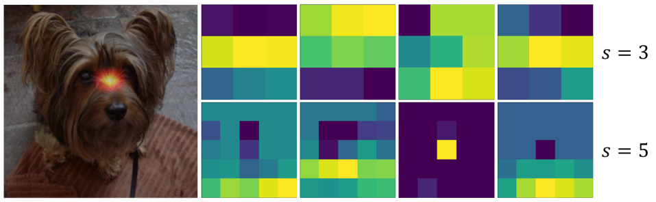
Figure 4: Exemplar templates of learned dictionary $D_{p}$. The templates shown are for randomly sampled channels for scale $3$ (top) and $5$ (bottom).

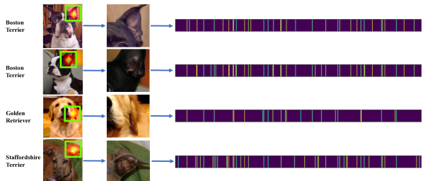
Figure 5: Template coefficients $z_{p}$ of the same part for two Boston Terriers (top 2 rows), a Golden Retriever (3rd row) and a Staffordshire Terrier (4th row). Template coefficients for images of the same class are similar. Visually-similar classes (Boston Terrier and Staffordshire Terrier) share some of the same activated templates, while visually distinct classes (Golden Retriever) differ a lot on their selection of active templates.

References

- Afrasiyabi et al. (2021) Arman Afrasiyabi, Jean-Francois Lalonde, and Christian Gagne. Mixture-based feature space learning for few-shot image classification. In Proceedings of the IEEE/CVF International Conference on Computer Vision, pp. 9041–9051, 2021.
- Baik et al. (2021) Sungyong Baik, Janghoon Choi, Heewon Kim, Dohee Cho, Jaesik Min, and Kyoung Mu Lee. Meta-learning with task-adaptive loss function for few-shot learning. In Proceedings of the IEEE/CVF International Conference on Computer Vision, pp. 9465–9474, 2021.
- Bateni et al. (2020) Peyman Bateni, Raghav Goyal, Vaden Masrani, Frank Wood, and Leonid Sigal. Improved few-shot visual classification. In Proceedings of the IEEE/CVF Conference on Computer Vision and Pattern Recognition, pp. 14493–14502, 2020.
- Bau et al. (2017) David Bau, Bolei Zhou, Aditya Khosla, Aude Oliva, and Antonio Torralba. Network dissection: Quantifying interpretability of deep visual representations. In Proceedings of the IEEE conference on computer vision and pattern recognition, pp. 6541–6549, 2017.
- Biederman (1987) Irving Biederman. Recognition-by-components: a theory of human image understanding. Psychological review, 94(2):115, 1987.
- Cao et al. (2020) Kaidi Cao, Maria Brbic, and Jure Leskovec. Concept learners for few-shot learning. arXiv preprint arXiv:2007.07375, 2020.
- Chen et al. (2021) Chaofan Chen, Xiaoshan Yang, Changsheng Xu, Xuhui Huang, and Zhe Ma. Eckpn: Explicit class knowledge propagation network for transductive few-shot learning. In Proceedings of the IEEE/CVF Conference on Computer Vision and Pattern Recognition, pp. 6596–6605, 2021.
- Chen et al. (2019) Wei-Yu Chen, Yen-Cheng Liu, Zsolt Kira, Yu-Chiang Frank Wang, and Jia-Bin Huang. A closer look at few-shot classification. arXiv preprint arXiv:1904.04232, 2019.
- Das et al. (2021) Rajshekhar Das, Yu-Xiong Wang, and Jose MF Moura. On the importance of distractors for few-shot classification. In Proceedings of the IEEE/CVF International Conference on Computer Vision, pp. 9030–9040, 2021.
- Doersch et al. (2020) Carl Doersch, Ankush Gupta, and Andrew Zisserman. Crosstransformers: spatially-aware few-shot transfer. Advances in Neural Information Processing Systems, 33:21981–21993, 2020.
- Everitt (1998) Brian Everitt. Cambridge dictionary of statistics. 1998.
- Fei et al. (2021) Nanyi Fei, Yizhao Gao, Zhiwu Lu, and Tao Xiang. Z-score normalization, hubness, and few-shot learning. In Proceedings of the IEEE/CVF International Conference on Computer Vision, pp. 142–151, 2021.
- Felzenszwalb et al. (2009) Pedro F Felzenszwalb, Ross B Girshick, David McAllester, and Deva Ramanan. Object detection with discriminatively trained part-based models. IEEE transactions on pattern analysis and machine intelligence, 32(9):1627–1645, 2009.
- Felzenszwalb et al. (2010) Pedro F Felzenszwalb, Ross B Girshick, and David McAllester. Cascade object detection with deformable part models. In 2010 IEEE Computer society conference on computer vision and pattern recognition, pp. 2241–2248. Ieee, 2010.
- Finn et al. (2017) Chelsea Finn, Pieter Abbeel, and Sergey Levine. Model-agnostic meta-learning for fast adaptation of deep networks. In International Conference on Machine Learning, pp. 1126–1135. PMLR, 2017.
- Girshick et al. (2015) Ross Girshick, Forrest Iandola, Trevor Darrell, and Jitendra Malik. Deformable part models are convolutional neural networks. In Proceedings of the IEEE conference on Computer Vision and Pattern Recognition, pp. 437–446, 2015.
- Gonzalez & Woods (2008) Rafael C. Gonzalez and Richard E. Woods. Digital image processing. Prentice Hall, Upper Saddle River, N.J., 2008.
- Hao et al. (2019) Fusheng Hao, Fengxiang He, Jun Cheng, Lei Wang, Jianzhong Cao, and Dacheng Tao. Collect and select: Semantic alignment metric learning for few-shot learning. In Proceedings of the IEEE/CVF International Conference on Computer Vision, pp. 8460–8469, 2019.
- Hastie et al. (2001) Trevor Hastie, Robert Tibshirani, and Jerome Friedman. The Elements of Statistical Learning. Springer Series in Statistics. Springer New York Inc., New York, NY, USA, 2001.
- He et al. (2016) Kaiming He, Xiangyu Zhang, Shaoqing Ren, and Jian Sun. Deep residual learning for image recognition. In Proceedings of the IEEE conference on computer vision and pattern recognition, pp. 770–778, 2016.
- Hilliard et al. (2018) Nathan Hilliard, Lawrence Phillips, Scott Howland, Artëm Yankov, Courtney D Corley, and Nathan O Hodas. Few-shot learning with metric-agnostic conditional embeddings. arXiv preprint arXiv:1802.04376, 2018.
- Jiang et al. (2020) Zihang Jiang, Bingyi Kang, Kuangqi Zhou, and Jiashi Feng. Few-shot classification via adaptive attention. arXiv preprint arXiv:2008.02465, 2020.
- Kang et al. (2021) Dahyun Kang, Heeseung Kwon, Juhong Min, and Minsu Cho. Relational embedding for few-shot classification. In Proceedings of the IEEE/CVF International Conference on Computer Vision, pp. 8822–8833, 2021.
- Khosla et al. (2011) Aditya Khosla, Nityananda Jayadevaprakash, Bangpeng Yao, and Li Fei-Fei. Novel dataset for fine-grained image categorization. In First Workshop on Fine-Grained Visual Categorization, IEEE Conference on Computer Vision and Pattern Recognition, Colorado Springs, CO, June 2011.
- Kingma & Ba (2014) Diederik P Kingma and Jimmy Ba. Adam: A method for stochastic optimization. arXiv preprint arXiv:1412.6980, 2014.
- Krause et al. (2013) Jonathan Krause, Michael Stark, Jia Deng, and Li Fei-Fei. 3d object representations for fine-grained categorization. In 4th International IEEE Workshop on 3D Representation and Recognition (3dRR-13), Sydney, Australia, 2013.
- Lee et al. (2019) Kwonjoon Lee, Subhransu Maji, Avinash Ravichandran, and Stefano Soatto. Meta-learning with differentiable convex optimization. In Proceedings of the IEEE/CVF Conference on Computer Vision and Pattern Recognition, pp. 10657–10665, 2019.
- Lee et al. (2022) SuBeen Lee, WonJun Moon, and Jae-Pil Heo. Task discrepancy maximization for fine-grained few-shot classification. In Proceedings of the IEEE/CVF Conference on Computer Vision and Pattern Recognition, pp. 5331–5340, 2022.
- Li et al. (2020a) Aoxue Li, Weiran Huang, Xu Lan, Jiashi Feng, Zhenguo Li, and Liwei Wang. Boosting few-shot learning with adaptive margin loss. In Proceedings of the IEEE/CVF Conference on Computer Vision and Pattern Recognition, pp. 12576–12584, 2020a.
- Li et al. (2020b) Kai Li, Yulun Zhang, Kunpeng Li, and Yun Fu. Adversarial feature hallucination networks for few-shot learning. In Proceedings of the IEEE/CVF Conference on Computer Vision and Pattern Recognition, pp. 13470–13479, 2020b.
- Li et al. (2019) Wenbin Li, Lei Wang, Jinglin Xu, Jing Huo, Yang Gao, and Jiebo Luo. Revisiting local descriptor based image-to-class measure for few-shot learning. In Proceedings of the IEEE/CVF Conference on Computer Vision and Pattern Recognition, pp. 7260–7268, 2019.
- Li et al. (2020c) Xiaoxu Li, Jijie Wu, Zhuo Sun, Zhanyu Ma, Jie Cao, and Jing-Hao Xue. Bsnet: Bi-similarity network for few-shot fine-grained image classification. IEEE Transactions on Image Processing, 30:1318–1331, 2020c.
- Li et al. (2017) Zhenguo Li, Fengwei Zhou, Fei Chen, and Hang Li. Meta-sgd: Learning to learn quickly for few-shot learning. arXiv preprint arXiv:1707.09835, 2017.
- Lifchitz et al. (2021) Yann Lifchitz, Yannis Avrithis, and Sylvaine Picard. Few-shot few-shot learning and the role of spatial attention. In 2020 25th International Conference on Pattern Recognition (ICPR), pp. 2693–2700. IEEE, 2021.
- Liu et al. (2018) Q Sun Y Liu, TS Chua, and B Schiele. Meta-transfer learning for few-shot learning. In 2018 IEEE Conference on Computer Vision and Pattern Recognition (CVPR), 2018.
- Maji et al. (2013) Subhransu Maji, Esa Rahtu, Juho Kannala, Matthew Blaschko, and Andrea Vedaldi. Fine-grained visual classification of aircraft. arXiv preprint arXiv:1306.5151, 2013.
- Rajeswaran et al. (2019) Aravind Rajeswaran, Chelsea Finn, Sham Kakade, and Sergey Levine. Meta-learning with implicit gradients. 2019.
- Rizve et al. (2021) Mamshad Nayeem Rizve, Salman Khan, Fahad Shahbaz Khan, and Mubarak Shah. Exploring complementary strengths of invariant and equivariant representations for few-shot learning. In Proceedings of the IEEE/CVF Conference on Computer Vision and Pattern Recognition, pp. 10836–10846, 2021.
- Savalle et al. (2014) Pierre-André Savalle, Stavros Tsogkas, George Papandreou, and Iasonas Kokkinos. Deformable part models with cnn features. In European Conference on Computer Vision, Parts and Attributes Workshop, 2014.
- Schwartz et al. (2018) Eli Schwartz, Leonid Karlinsky, Joseph Shtok, Sivan Harary, Mattias Marder, Rogerio Feris, Abhishek Kumar, Raja Giryes, and Alex M Bronstein. Delta-encoder: an effective sample synthesis method for few-shot object recognition. arXiv preprint arXiv:1806.04734, 2018.
- Simon et al. (2020) Christian Simon, Piotr Koniusz, Richard Nock, and Mehrtash Harandi. Adaptive subspaces for few-shot learning. In Proceedings of the IEEE/CVF Conference on Computer Vision and Pattern Recognition, pp. 4136–4145, 2020.
- Snell et al. (2017) Jake Snell, Kevin Swersky, and Richard S Zemel. Prototypical networks for few-shot learning. arXiv preprint arXiv:1703.05175, 2017.
- Sun et al. (2020) Xin Sun, Hongwei Xv, Junyu Dong, Huiyu Zhou, Changrui Chen, and Qiong Li. Few-shot learning for domain-specific fine-grained image classification. IEEE Transactions on Industrial Electronics, 68(4):3588–3598, 2020.
- Sung et al. (2018) Flood Sung, Yongxin Yang, Li Zhang, Tao Xiang, Philip HS Torr, and Timothy M Hospedales. Learning to compare: Relation network for few-shot learning. In Proceedings of the IEEE conference on computer vision and pattern recognition, pp. 1199–1208, 2018.
- Tang et al. (2020) Luming Tang, Davis Wertheimer, and Bharath Hariharan. Revisiting pose-normalization for fine-grained few-shot recognition. In Proceedings of the IEEE/CVF Conference on Computer Vision and Pattern Recognition, pp. 14352–14361, 2020.
- Tokmakov et al. (2019) Pavel Tokmakov, Yu-Xiong Wang, and Martial Hebert. Learning compositional representations for few-shot recognition. In Proceedings of the IEEE/CVF International Conference on Computer Vision, pp. 6372–6381, 2019.
- Ullman et al. (2002) Shimon Ullman, Michel Vidal-Naquet, and Erez Sali. Visual features of intermediate complexity and their use in classification. Nature neuroscience, 5(7):682–687, 2002.
- Van Trees (2004) Harry L Van Trees. Detection, estimation, and modulation theory, part I: detection, estimation, and linear modulation theory. John Wiley & Sons, 2004.
- Vinyals et al. (2016) Oriol Vinyals, Charles Blundell, Timothy Lillicrap, Daan Wierstra, et al. Matching networks for one shot learning. Advances in neural information processing systems, 29:3630–3638, 2016.
- Wah et al. (2011) C. Wah, S. Branson, P. Welinder, P. Perona, and S. Belongie. The Caltech-UCSD Birds-200-2011 Dataset. Technical Report CNS-TR-2011-001, California Institute of Technology, 2011.
- Wang et al. (2021) Chaofei Wang, Shiji Song, Qisen Yang, Xiang Li, and Gao Huang. Fine-grained few shot learning with foreground object transformation. Neurocomputing, 466:16–26, 2021.
- Wang et al. (2019) Yan Wang, Wei-Lun Chao, Kilian Q Weinberger, and Laurens van der Maaten. Simpleshot: Revisiting nearest-neighbor classification for few-shot learning. arXiv preprint arXiv:1911.04623, 2019.
- Wang et al. (2018) Yu-Xiong Wang, Ross Girshick, Martial Hebert, and Bharath Hariharan. Low-shot learning from imaginary data. In Proceedings of the IEEE conference on computer vision and pattern recognition, pp. 7278–7286, 2018.
- Wertheimer et al. (2021) Davis Wertheimer, Luming Tang, and Bharath Hariharan. Few-shot classification with feature map reconstruction networks. In Proceedings of the IEEE/CVF Conference on Computer Vision and Pattern Recognition, pp. 8012–8021, 2021.
- Wu et al. (2021) Jiamin Wu, Tianzhu Zhang, Yongdong Zhang, and Feng Wu. Task-aware part mining network for few-shot learning. In Proceedings of the IEEE/CVF International Conference on Computer Vision, pp. 8433–8442, 2021.
- Xu et al. (2021) Jingyi Xu, Hieu Le, Mingzhen Huang, ShahRukh Athar, and Dimitris Samaras. Variational feature disentangling for fine-grained few-shot classification. In Proceedings of the IEEE/CVF International Conference on Computer Vision, pp. 8812–8821, 2021.
- Yang et al. (2020) Ling Yang, Liangliang Li, Zilun Zhang, Xinyu Zhou, Erjin Zhou, and Yu Liu. Dpgn: Distribution propagation graph network for few-shot learning. In Proceedings of the IEEE/CVF Conference on Computer Vision and Pattern Recognition, pp. 13390–13399, 2020.
- Ye et al. (2020) Han-Jia Ye, Hexiang Hu, De-Chuan Zhan, and Fei Sha. Few-shot learning via embedding adaptation with set-to-set functions. In Proceedings of the IEEE/CVF Conference on Computer Vision and Pattern Recognition, pp. 8808–8817, 2020.
- Zhang et al. (2021) Baoquan Zhang, Xutao Li, Yunming Ye, Zhichao Huang, and Lisai Zhang. Prototype completion with primitive knowledge for few-shot learning. In Proceedings of the IEEE/CVF Conference on Computer Vision and Pattern Recognition, pp. 3754–3762, 2021.
- Zhang et al. (2020) Chi Zhang, Yujun Cai, Guosheng Lin, and Chunhua Shen. Deepemd: Few-shot image classification with differentiable earth mover’s distance and structured classifiers. In Proceedings of the IEEE/CVF conference on computer vision and pattern recognition, pp. 12203–12213, 2020.
- Zheng et al. (2017) Heliang Zheng, Jianlong Fu, Tao Mei, and Jiebo Luo. Learning multi-attention convolutional neural network for fine-grained image recognition. In 2017 IEEE International Conference on Computer Vision (ICCV), pp. 5209–5217, 2017. doi: 10.1109/ICCV.2017.557.
- Zhou et al. (2014) Bolei Zhou, Aditya Khosla, Agata Lapedriza, Aude Oliva, and Antonio Torralba. Object detectors emerge in deep scene cnns. arXiv preprint arXiv:1412.6856, 2014.
- Zhou et al. (2021) Ziqi Zhou, Xi Qiu, Jiangtao Xie, Jianan Wu, and Chi Zhang. Binocular mutual learning for improving few-shot classification. In Proceedings of the IEEE/CVF International Conference on Computer Vision, pp. 8402–8411, 2021.
- Zhu et al. (2020) Yaohui Zhu, Chenlong Liu, and Shuqiang Jiang. Multi-attention meta learning for few-shot fine-grained image recognition. In IJCAI, pp. 1090–1096, 2020.