Convolutional Bypasses Are Better Vision Transformer Adapters

Abstract

The pretrain-then-finetune paradigm has been widely adopted in computer vision. But as the size of Vision Transformer (ViT) grows exponentially, the full finetuning becomes prohibitive in view of the heavier storage overhead. Motivated by parameter-efficient transfer learning (PETL) on language transformers, recent studies attempt to insert lightweight adaptation modules (e.g., adapter layers or prompt tokens) to pretrained ViT and only finetune these modules while the pretrained weights are frozen. However, these modules were originally proposed to finetune language models and did not take into account the prior knowledge specifically for visual tasks. In this paper, we propose to construct Convolutional Bypasses (Convpass) in ViT as adaptation modules, introducing only a small amount (less than 0.5% of model parameters) of trainable parameters to adapt the large ViT. Different from other PETL methods, Convpass benefits from the hard-coded inductive bias of convolutional layers and thus is more suitable for visual tasks, especially in the low-data regime. Experimental results on VTAB-1K benchmark and few-shot learning datasets show that Convpass outperforms current language-oriented adaptation modules, demonstrating the necessity to tailor vision-oriented adaptation modules for adapting vision models.

1 Introduction

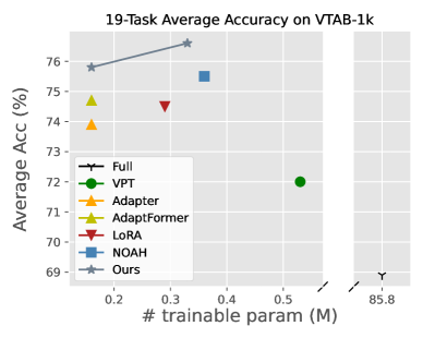
Figure 1: Average accuracy vs. number of trainable parameters on VTAB-1K benchmark. Our vision-oriented Convpass outperforms other language-oriented methods.

Pretraining on large-scale datasets (e.g., ImageNet) and then fully finetuning on downstream tasks has become the de-facto paradigm to achieve state-of-the-art (SOTA) performance on visual tasks (Kolesnikov et al. 2020). However, this paradigm is not storage-efficient – it requires one to store a whole model for each downstream task. Recently, as Vision Transformer (ViT) (Dosovitskiy et al. 2021) dominates vision field gradually, the size of vision models has grown exponentially (58M of ResNet-152 (He et al. 2016) vs. 1843M of ViT-G (Zhai et al. 2022)), which creates the demand for parameter-efficient transfer learning (PETL) on ViT.

Fortunately, since transformer was first adopted in neural language processing (NLP) (Vaswani et al. 2017), PETL on large pretrained language models has been studied sufficiently (Houlsby et al. 2019; Hu et al. 2022; Li and Liang 2021; He et al. 2022a), which can be easily ported to ViT. Concretely, these PETL methods insert lightweight adaptation modules into the pertrained models, freeze the pretrained weights, and finetune these modules end-to-end to adapt to downstream tasks. Recent work has verified the effectiveness of these PETL methods on ViT (Jia et al. 2022; Zhang, Zhou, and Liu 2022), but we raise a question: Are these modules designed for the language models optimal for vision models as well?

It is known that NLP tasks and visual tasks desire different inductive bias, which profoundly affects the model architecture design. By analyzing current PETL methods from an unraveled perspective, we argue that these methods, called “language-oriented modules”, also imply the inductive bias for language, e.g., weak spatial relation and support for variable-length input. Therefore, a better adaptation module for ViT should also reflect visual inductive bias, such as spatial locality and 2D neighborhood structure, which is referred to as “vision-oriented modules”.

When a model (e.g., ViT) has weak inductive bias, it needs a large amount of data to learn the inductive bias from scratch. This may not be a serious problem in the pretraining process, since we can leverage easily accessible unlabeled data for self-supervised learning (Bao, Dong, and Wei 2022; He et al. 2022b), or resort to multi-modal pretraining (Radford et al. 2021; Yu et al. 2022). However, data of downstream tasks is usually collected from specific domains that may be expensive or hard to acquire. Therefore, besides the inductive bias learned from pretraining data, a well-designed vision-oriented PETL module is expected to introduce additional inductive bias and improve data efficiency much further.

In this paper, we propose to construct Convolutional Bypasses (Convpass) in ViT as adaptation modules. Convpass is an inserted convolutional bottleneck block parallel to the MHSA or MLP block, which “bypasses” the original ViT block. It reconstructs the spatial structure of the token sequence and performs convolution on image tokens and [cls] token individually. During finetuning, only these Convpass modules and the classification head are updated. Due to the hard-coded locality of convolutional layers, Convpass can capture visual information more efficiently, especially when the downstream data is limited. As shown in Figure 1, Convpass only introduces and tunes about 0.33M new parameters for a ViT-B of 86M, while achieving better performance than both full finetuning and current SOTA language-oriented methods on 19-task VTAB benchmark (Zhai et al. 2019). Further experiments on few-shot learning demonstrate that Convpass also outperforms other baselines in the low-data regime, and can be directly used on vision-language model (Radford et al. 2021) with good domain generalization performance.

We summarize the contributions as follows:

• We point out the weak visual inductive bias of current PETL methods that limits their performance on ViT.

• We propose Convpass, a simple yet effective PETL method which leverages trainable convolutional blocks as bypasses to adapt pretrained ViT to downstream visual tasks.

• Experimental results show that Convpass outperforms previous language-oriented methods, indicating the necessity to tailor vision-oriented adaptation modules for vision models.

2 Related Work

2.1 Vision Transformer

Transformer-based models have achieved great success in NLP (Devlin et al. 2019; Raffel et al. 2020; Brown et al. 2020). ViT adopts this architecture in visual tasks by partitioning the images into patches which are embedded and flattened into 1D token sequences.

In ViT, each layer consists of two kinds of blocks: Multi-Head Self-Attention (MHSA) and Multi-Layer Perceptron (MLP). In an MHSA block, the input sequence $\boldsymbol{X}\in\mathbb{R}^{N\times d}$ is firstly projected to query $\boldsymbol{Q}=\boldsymbol{XW}_{q}$, key $\boldsymbol{K}=\boldsymbol{XW}_{k}$, and value $\boldsymbol{V}=\boldsymbol{XW}_{v}$, respectively, in which $\boldsymbol{W}_{q/k/v}\in\mathbb{R}^{d\times d}$. They are further divided into $N_{h}$ heads: $\{\boldsymbol{Q}^{(i)}\}^{N_{h}}_{i=1},\{\boldsymbol{K}^{(i)}\}^{N_{h}}_{i=1},\{\boldsymbol{V}^{(i)}\}^{N_{h}}_{i=1}$. Then, the self-attention of a single head is formulated as

$$\textit{Attn-Head}^{(i)}(\boldsymbol{X})=\textit{Softmax}\left(\frac{\boldsymbol{Q}^{(i)}{\boldsymbol{K}^{(i)}}^{\intercal}}{\sqrt{d}}\right)\boldsymbol{V}^{(i)}$$

The outputs of all heads are further concatenated and linearly projected as the outputs of the MHSA block.

An MLP block consists of two fully-connected (FC) layers, whose weights are $\boldsymbol{W}_{1}\in\mathbb{R}^{d\times D}$ and $\boldsymbol{W}_{2}\in\mathbb{R}^{D\times d}$, respectively. Ignoring the bias parameters for simplicity, the MLP is formulated as

$$\textit{MLP}(\boldsymbol{X})=\textit{GELU}(\boldsymbol{X}\boldsymbol{W}_{1})\boldsymbol{W}_{2}$$

Since ViT has much less visual inductive bias, it performs worse than its convolutional counterparts (e.g., ResNet) when the training data is not sufficient. For this reason, some recent work proposes to introduce visual inductive bias into ViT (Liu et al. 2021b; Wu et al. 2021), which significantly reduces its dependency on scale of dataset. However, vanilla ViT still has some nonnegligible advantages. Since vanilla ViT shares the same backbone as the transformer-based language models, it can leverage current SOTA multi-modal pretraining methods with a vast amount of auto-annotated image-text pairs (Wang et al. 2021; Yu et al. 2022). Therefore, we still focus on PETL on vanilla ViT architecture, but propose to introduce hard-coded inductive bias by adaptation modules during finetuning instead of pretraining.

2.2 Parameter-Efficient Transfer Learning

PETL aims at using a small number of trainable parameters to adapt large models to downstream tasks. We here introduce some common PETL methods used for ViT.

Adapter (Houlsby et al. 2019; Pfeiffer et al. 2021) is a bottleneck MLP block composed of two fully connected layers, whose weights are $\boldsymbol{W}_{down}\in\mathbb{R}^{d\times h}$ and $\boldsymbol{W}_{up}\in\mathbb{R}^{h\times d}$, where $h<<d$. Adapters are inserted into networks as residual connections, i.e., given an input $\boldsymbol{X}\in\mathbb{R}^{N\times d}$, the computation is formulated as

$$\boldsymbol{X}^{\prime}\leftarrow\boldsymbol{X}+\phi(\boldsymbol{X}\boldsymbol{W}_{down})\boldsymbol{W}_{up}$$

where $\phi$ is activation function such as GELU.

Pfeiffer et al. (2021) propose to place Adapters after the MLP blocks (i.e., $\boldsymbol{X}$ is the output of MLP blocks), which has been proved to be an efficient design in previous literature (Hu et al. 2022), so we follow this setting in this paper. Besides the above design, He et al. (2022a) and Chen et al. (2022) also propose a parallel Adapter to adapt MLP blocks, which is formulated as

$$\boldsymbol{X}^{\prime}\leftarrow\boldsymbol{X}+\textit{MLP}(\boldsymbol{X})+s\cdot\phi(\boldsymbol{X}\boldsymbol{W}_{down})\boldsymbol{W}_{up}$$

where $s$ is a hyperparameter, $\boldsymbol{X}$ is the input of MLP blocks. This Adapter design is referred to as AdaptFormer by Chen et al. (2022).

LoRA (Hu et al. 2022) learns the low-rank approximation of increments of $\boldsymbol{W}_{q}$ and $\boldsymbol{W}_{v}$. Formally, it decomposes $\Delta\boldsymbol{W}_{q/v}$ into $\boldsymbol{A}_{q/v}\boldsymbol{B}_{q/v}$, where $\boldsymbol{A}_{q/v}\in\mathbb{R}^{d\times r},\boldsymbol{B}_{q/v}\in\mathbb{R}^{r\times d}$ and $r<<d$. The query and key are computed as

$$\boldsymbol{Q/K}=\boldsymbol{XW}_{q/k}+s\cdot\boldsymbol{XA}_{q/k}\boldsymbol{B}_{q/k}$$

in which $s$ is a scaling hyperparameter.

VPT (Jia et al. 2022) has a similar idea with P-Tuning v2 (Liu et al. 2021a). It concatenates the input $\boldsymbol{X}$ with several trainable prompts $\boldsymbol{P}\in\mathbb{R}^{l\times d}$ before each layer. This extended sequence is formulated as

$$\boldsymbol{X}^{\prime}\leftarrow[\boldsymbol{X},\boldsymbol{P}]$$

These prompts are then cut away at the end of a layer, and the prompts for the next layer are concatenated.

NOAH (Zhang, Zhou, and Liu 2022) is a newly proposed PETL method for ViT, which combines the above three modules together and performs neural architecture search on hidden dimension $h$ of Adapter, rank $r$ of LoRA, and prompt length $l$ of VPT.

Note that although VPT and NOAH are proposed for visual tasks, their components are ported from NLP in essence. Therefore, all the aforementioned PETL methods can be classified as language-oriented methods. Other PETL methods such as BitFit (Zaken, Goldberg, and Ravfogel 2022), which finetunes the bias parameters only; and Sidetune (Zhang et al. 2020), which finetunes a small side-network and interpolates between pretrained and side-tuned features, have been proved to perform rather poorly on ViT by Jia et al. (2022).

3 Methodology

3.1 Rethinking Adapters from an Unraveled View

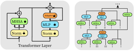
Figure 2: Illustration of the unraveled view of ViT equipped with Adapter. For simplicity, we show the unraveled view of a fragment of ViT (MHSA-MLP-MHSA) and the type of each path. Normalization layers are omitted.

Since Adapters and MHSA/MLP blocks all contain skip connections, we can unravel the ViT and rewrite it as a collection of paths. Veit, Wilber, and Belongie (2016) point out that the original network is an ensemble of unraveled paths, so we here give a look at these paths to analyze the property of the original network.

As shown in Figure 2, a ViT equipped with Adapter can be viewed as an ensemble of three types of paths: (Type I) Frozen paths, which only contain MHSA/MLP blocks of the ViT. These paths are not trainable, and the sum of their outputs is identically equal to the output of the pretrained ViT. (Type II) MHSA-Adapter paths, where all MHSA blocks come before the first Adapter. (Type III) Adapter-MHSA paths, where at least one MHSA block is placed after an Adapter.

Finetuning the Adapters is equivalent to fitting the changes of outputs by the paths of Type II & III. In Type II paths, given the same input, the output tokens of the last MHSA blocks are unchanged, and there is no information exchange between tokens after that. Therefore, only the Type III paths, in fact, make changes to the token mixer of the pretrained ViT.

In a Type III paths, we can treat all Adapters and MLP blocks before an MHSA block as a part of its query/key/value transformation, i.e., complicate these transformations form linear mapping to

$$\boldsymbol{Q/K/V}=f_{q/k/v}(\boldsymbol{X})$$

where $f_{q/k/v}$ are channel-wise MLPs. Therefore, finetuning Type III paths can be considered as finetuning the MHSA with the complicated query/key/value transformations.

Meanwhile, since LoRA finetunes $\boldsymbol{W}_{q/v}$ in a low-rank subspace and VPT can be regarded as parallel and gated Adapters (He et al. 2022a), all these language-oriented methods rely on tuning MHSA to adjust the token mixer on downstream tasks. MHSA, however, lacks visual inductive bias, which may perform poorly when the data of downstream visual tasks is limited.

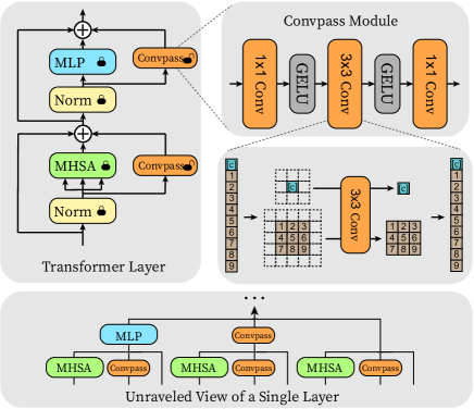
Figure 3: Overview of the proposed method. We restore the spatial structure of the token sequence, and use trainable ResNet-style convolutional blocks as bypasses. The [cls] token is regarded as an individual image.

		Natural							Specialized				Structured
	# param (M)	Cifar100	Caltech101	DTD	Flower102	Pets	SVHN	Sun397	Camelyon	EuroSAT	Resisc45	Retinopathy	Clevr-Count	Clevr-Dist	DMLab	KITTI-Dist	dSpr-Loc	dSpr-Ori	sNORB-Azim	sNORB-Ele	Average
Traditional Finetuning
Full	85.8	68.9	87.7	64.3	97.2	86.9	87.4	38.8	79.7	95.7	84.2	73.9	56.3	58.6	41.7	65.5	57.5	46.7	25.7	29.1	68.9
Linear	0	64.4	85.0	63.2	97.0	86.3	36.6	51.0	78.5	87.5	68.5	74.0	34.3	30.6	33.2	55.4	12.5	20.0	9.6	19.2	57.6
PETL methods
VPT	0.53	78.8	90.8	65.8	98.0	88.3	78.1	49.6	81.8	96.1	83.4	68.4	68.5	60.0	46.5	72.8	73.6	47.9	32.9	37.8	72.0
Adapter	0.16	69.2	90.1	68.0	98.8	89.9	82.8	54.3	84.0	94.9	81.9	75.5	80.9	65.3	48.6	78.3	74.8	48.5	29.9	41.6	73.9
AdaptFormer	0.16	70.8	91.2	70.5	99.1	90.9	86.6	54.8	83.0	95.8	84.4	76.3	81.9	64.3	49.3	80.3	76.3	45.7	31.7	41.1	74.7
LoRA	0.29	67.1	91.4	69.4	98.8	90.4	85.3	54.0	84.9	95.3	84.4	73.6	82.9	69.2	49.8	78.5	75.7	47.1	31.0	44.0	74.5
NOAH	0.36	69.6	92.7	70.2	99.1	90.4	86.1	53.7	84.4	95.4	83.9	75.8	82.8	68.9	49.9	81.7	81.8	48.3	32.8	44.2	75.5
Convpass${}_{\textit{attn}}$	0.16	71.8	90.7	72.0	99.1	91.0	89.9	54.2	85.2	95.6	83.4	74.8	79.9	67.0	50.3	79.9	84.3	53.2	34.8	43.0	75.8
Convpass	0.33	72.3	91.2	72.2	99.2	90.9	91.3	54.9	84.2	96.1	85.3	75.6	82.3	67.9	51.3	80.0	85.9	53.1	36.4	44.4	76.6

Table 1: Full results on the VTAB-1K benchmark. “Average” denotes the average results over three group-wise averages in Figure 4. “# params” denotes the average number of trainable parameters in backbones. Convpass(-attn) achieves 12 SOTA results out of the 19 tasks among PETL methods.

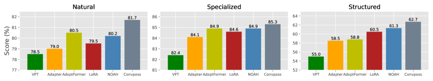
Figure 4: Group-wise average results on VTAB-1K. Convpass outperforms other baselines in all of the three groups.

3.2 Adapting ViT via Convolutional Bypasses

Recent studies on modifying the architecture of ViT have verified that introducing convolution into ViT will improve the performance when training data is not adequate (Dosovitskiy et al. 2021; Wu et al. 2021). Since the data of downstream tasks is usually limited even few-shot, we can also introduce convolution into the adaptation modules for PETL.

As illustrated in Figure 3, a Convpass module consists of three convolutional layers: an $1\times 1$ convolution reducing the channel, a $3\times 3$ convolution with the same input and output channel, and an $1\times 1$ convolution expanding the channel. Since ViT flattens the image into an 1D token sequence, we restore the 2D structure before convolution. The [cls] token serves as an individual image. The Convpass modules are placed parallel to the MHSA/MLP blocks, which can be formulated as

$$\boldsymbol{X}^{\prime}\leftarrow\boldsymbol{X}+\textit{MHSA/MLP}(\textit{LN}(\boldsymbol{X}))+s\cdot\textit{Convpass}(\textit{LN}(\boldsymbol{X}))$$

where $s$ is a hyperparameter and LN is Layer Normalization (Ba, Kiros, and Hinton 2016). Note that the Convpass modules are similar to the residual bottleneck blocks of ResNet (He et al. 2016). If we ignore the MHSA/MLP blocks, the ViT will turn into a ResNet-like CNN.

From the unraveled view, we can find that in each transformer layer, besides the frozen paths, there are also trainable paths that only contain Convpass or contain both Convpass and MHSA which act as token-mixers. Therefore, the original transformer layers are converted to an ensemble of transformers, ResNet-like CNNs, and hybrid models. This design can help transfer learning from several perspective. First, since all the trainable paths contain Convpass modules, the finetuning process can benefit from the inherent visual inductive bias of CNN. Second, the 2D neighborhood structure of the $3\times 3$ convolution focuses on local information, complementary to the MHSA that has global receptive field.

Convpass is storage-efficient. If the bottleneck channel size (i.e., the input & output channel of the $3\times 3$ convolution) is denoted as $h$, and the amount of ViT layers is $L$, the number of trainable parameters is $2L\times\left((2h+1)d+9h^{2}+2h\right)$. In view of $h<<d$ (e.g., $d=768,h=8$ in our experiments), this amount is $\mathcal{O}(Ld)$, which is negligible compared to ViT’s $\mathcal{O}(Ld^{2})$ parameters.

4 Experiments

4.1 Transfer Learning on VTAB-1K Benchmark

First of all, our method is evaluated on the basic transfer learning scenario – finetuning the pretrained models on various dowmstream tasks.

Datasets

To evaluate the performance on transfer learning of our methods, we use VTAB-1K (Zhai et al. 2019) as a benchmark. VTAB-1K benchmark contains 19 image classification tasks from different fields, which can be roughly categorized into three groups: Natural, Specialized, and Structured. Each classification task only has 1,000 training samples, which are split into a training set (800) and a validation set (200) during hyperparameter search. The reported results are produced by evaluating the model trained on all the 1,000 training samples on test set.

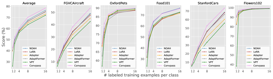
Figure 5: Results of few-shot learning on five fine-grained visual recognition datasets. Convpass outperforms other baselines on average results.

Baselines

We compare our method with two traditional finetuning methods: Full finetuning, which optimizes all parameters end-to-end; Linear evaluation, which freezes the pretrained backbone and only learns a classification head; as well as four PETL methods: VPT, Adapter, AdaptFormer, LoRA, and NOAH. For our method Convpass, we also report a simplified variant: Convpass${}_{\textit{attn}}$, which only inserts the Convpass modules alongside the MHSA blocks. Note that VPT, Adapter, LoRA, and Convpass only contain one type of PETL module, and the network architecture is the same for all tasks; while NOAH focuses on architecture search to combine other existing PETL modules, resulting in a dynamic network architecture.

Setup

We use a ViT-B/16 (Dosovitskiy et al. 2021) supervisedly pretrained on ImageNet-21K (Deng et al. 2009) for al methods. The networks are finetuned for 100 epochs except for NOAH, which also trains a supernet for another 500 epochs. The hidden dimension $h$ of Adapter, AdaptFormer and Convpass, as well as the rank $r$ of LoRA are all set to 8. The prompt length $l$ of VPT follows the best recipe in its original paper. The hyperparameter $s$ of Convpass and AdaptFormer is roughly searched from {0.01, 0.1, 1, 10, 100}. In this setting, Adapter, AdaptFormer and Convpass${}_{\textit{attn}}$ have similar numbers of trainable parameters, while the Convpass’s trainable parameters are slightly more than LoRA’s but fewer than VPT’s and NOAH’s. Other hyperparameters are listed in the Appendix.

Results

As shown in Table 1, Convpass${}_{\textit{attn}}$ outperforms its counterpart Adapter and AdaptFormer on 16 and 10 out of the 19 tasks, while Convpass outperforms its counterparts LoRA and NOAH on 15 and 13 tasks, respectively. Although using fewer parameters, Convpass still performs better than VPT on 17 tasks. All the PETL methods are better than full finetuning overall. Because of the variety of tasks, no one method achieves SOTA on all tasks at once, but Convpass achieves the best average performance, $1.1\%$ higher than the previous SOTA PETL methods, NOAH. It is worth noting that Convpass${}_{\textit{attn}}$ also has better average results than NOAH with only half as many parameters as NOAH. Moreover, since NOAH need to train an additional large supernet for architecture search, Convpass is also superior to NOAH in terms of training efficiency.

Figure 4 shows that Convpass has the best performance in all the three groups of VTAB, indicating that Convpass specializes in visual tasks from various domains. The superiority of Convpass is significant in the Natural and Structured groups. But in the Specialized group, Convpass does not remarkably outperform NOAH and AdaptFormer.

4.2 Few-Shot Learning

Few-shot learning is a common scenario when the data of downstream tasks is hard to obtain, and there are only a few training samples for each task that can be utilized.

Datasets

We use five fine-gained datasets to evaluate the performance of our methods on few-shot learning: FGVC-Aircraft (Maji et al. 2013a), Oxford-Pets (Parkhi et al. 2012), Food-101 (Bossard, Guillaumin, and Gool 2014), Stanford Cars (Krause et al. 2013), and Oxford-Flowers102 (Nilsback and Zisserman 2006). We conduct experiments on 1, 2, 4, 8, and 16 shot settings. The results are averaged over three runs with different seeds. The experimental setup and baselines are the same as for VTAB-1K.

Results

As shown in Figure 5, the average results of Convpass are all higher than the other baselines across the five settings. On FGVC-Aircraft and Stanford Cars, the advantages of Convpass are highlighted. On simpler Oxford-Pets and Oxford-Flowers102, all the methods have similar performance, while Convpass is still in the lead. On Food-101, Convpass slightly underperforms NOAH in the 16-shot case, but the trend is reversed when the number of training data gets smaller. These results demonstrate that the introduced inductive bias of Convpass enhances ViT’s capability to learn in the low-data regime.

4.3 Domain Generalization

Besides vision models, PETL has been studied in the field of vision-language models as well. Considering the outstanding domain generalization property of vision-language models, we also evaluate the performance of our method under domain shift when applied to vision-language models.

Datasets

In domain generalization experiments, the models are trained on the source domain, and tested on both the source and target domain. We use ImageNet-1K (Deng et al. 2009) as the source domain, where each class contains 16 training samples. The target domains include: ImageNet-V2 (Recht et al. 2019), which is a new ImageNet test set collected with the original labelling protocol; ImageNet-Sketch (Wang et al. 2019), which consists of sketch images of the 1,000 ImageNet classes; ImageNet-A (Hendrycks et al. 2021b), which contains real-world adversarial samples of 200 of the ImageNet classes; ImageNet-R (Hendrycks et al. 2021a), which is composed of renditions of 200 ImageNet classes.

Method	Source		Target
	ImageNet		-V2	-Sketch	-A	-R
ZS CLIP	66.73		60.83	46.15	47.77	73.96
LP CLIP	65.85		56.26	34.77	35.68	58.43
CoOp	71.51		64.20	47.99	49.71	75.21
CoCoOp	71.02		64.07	48.75	50.63	76.18
Tip-Adapter-F	73.41		65.39	48.58	49.23	77.54
Convpass${}_{\textit{CLIP}}$	74.23		66.61	49.10	49.27	78.17

Table 2: Results of 16-shot ImageNet classification and domain generalization on CLIP. We report top-1 accuracy. Convpass${}_{\textit{CLIP}}$ outperforms the baselines on source domain and three of the four target domains.

Baselines

The CLIP (Radford et al. 2021) model consists of an image encoder and a text encoder, which are pretrained via contrastive learning on image-text pairs. Our method is compared with the following baselines: Zero-Shot (ZS) CLIP uses prompted label texts (e.g., “A photo of <class name>.”) as the text encoder inputs, and classifies the images based on cosine similarity between image and text features ; Linear Probe (LP) CLIP discards the text encoder and learns a linear classification head for image encoder; CoOp (Zhou et al. 2021) makes use of trainable vectors as prompts of labels; CoCoOp (Zhou et al. 2022) learns a meta-net to generate prompts of labels from images; Tip-Adapter-F (Zhang et al. 2022) caches features of training data to initialize an adapter after the image encoder. Note that CoOp, CoCoOp, and Tip-Adapter-F are PETL methods designed for CLIP specifically.

To apply our methods to CLIP, we make the following modifications. First, we insert Convpass modules into the image encoder only, while the text encoder stays unchanged. Second, we add a FC layer as classification head of the image encoder, whose bias is zero-initialized and whose weight is initialized with encoded prompted label texts of all classes (just as in ZS CLIP). Then, the text encoder is discarded, and only the Convpass modules and head are finetuned. We call this ported PETL method Convpass${}_{\textit{CLIP}}$.

Setup

In our experiments, all methods use a ViT-B/16 as the image encoder, and a BERT-like (Devlin et al. 2019) model as the text encoder. For our methods, we train the Convpass modules and classification heads for 50 epochs. Other hyperparameters are listed in the Appendix.

Results

The results are shown in Table 2. Our method, though not designed for CLIP, still outperforms the baselines tailored for CLIP on the source domain. On three out of the four target domains, Convpass${}_{\textit{CLIP}}$ also achieves SOTA performance. On ImageNet-A, Convpass${}_{\textit{CLIP}}$ performs a bit poorly, which is probably because the ImageNet-A dataset is collected by selecting samples misclassified by ResNet. Since Convpass modules are ResNet-style blocks, they may be more easily misled by these samples as well. Overall, the results prove that Convpass${}_{\textit{CLIP}}$ is robust under domain shift.

Model	Method	Avg.	Nat.	Spe.	Str.
ConvNeXt-B	Full	74.0	78.0	83.7	60.4
ConvNeXt-B	Linear	63.6	74.5	81.5	34.8
Swin-B	Full	75.0	79.2	86.2	59.7
Swin-B	Linear	62.6	73.5	80.8	33.5
Swin-B	VPT	71.6	76.8	84.5	53.4
Swin-B	Convpass	78.1	83.1	87.2	64.1
ViT-B/16	Full	68.9	75.9	83.4	47.6
ViT-B/16	Linear	57.6	68.9	77.2	26.8
ViT-B/16	VPT	72.0	78.5	82.4	55.0
ViT-B/16	Convpass	76.6	81.7	85.3	62.7

Table 3: Results on VTAB-1K. ConvNeXt-B and Swin-B have inherent inductive bias for vision, while ViT introduces such inductive bias via Convpass during finetuning. Avg.: Average, Nat.: Natural, Spe.: Specialized, Str.: Structured.

4.4 Further Analyses

Comparison with Other Backbones

One of the motivations for designing Convpass is to introduce visual inductive bias to ViT during finetuning. However, since there are also ViT variants (e.g., Swin Transformer (Liu et al. 2021b)) which have already incorporated visual inductive bias into their model designs, finetuning on these models can naturally benefit from such prior knowledge. Then a question arises: Can the models that acquire inductive bias during finetuning outperform these models that have innately hard-coded inductive bias?

We conduct comparisons among the three backbone models: ViT-B/16, Swin-B (Liu et al. 2021b), and a SOTA CNN ConvNeXt-B (Liu et al. 2022). All of them are pretrained on ImageNet-21K and have a similar size. As the results shown in Table 3, when using traditional transfer learning methods (Full and Linear), Swin-B and ConvNeXt-B perform significantly better than ViT-B/16 as expected, which indicates the pivotal role of visual inductive bias during finetuning. However, when equipped with Convpass, the average performance of ViT-B/16 overtakes fully finetuned Swin-B and ConvNeXt-B. These observations suggest that Convpass has the powerful capability to complement the missing inductive bias for downstream transfer tasks.

(a) Convpass${}_{\textit{mlp}}$

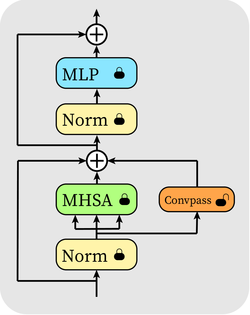
(b) Convpass${}_{\textit{attn}}$

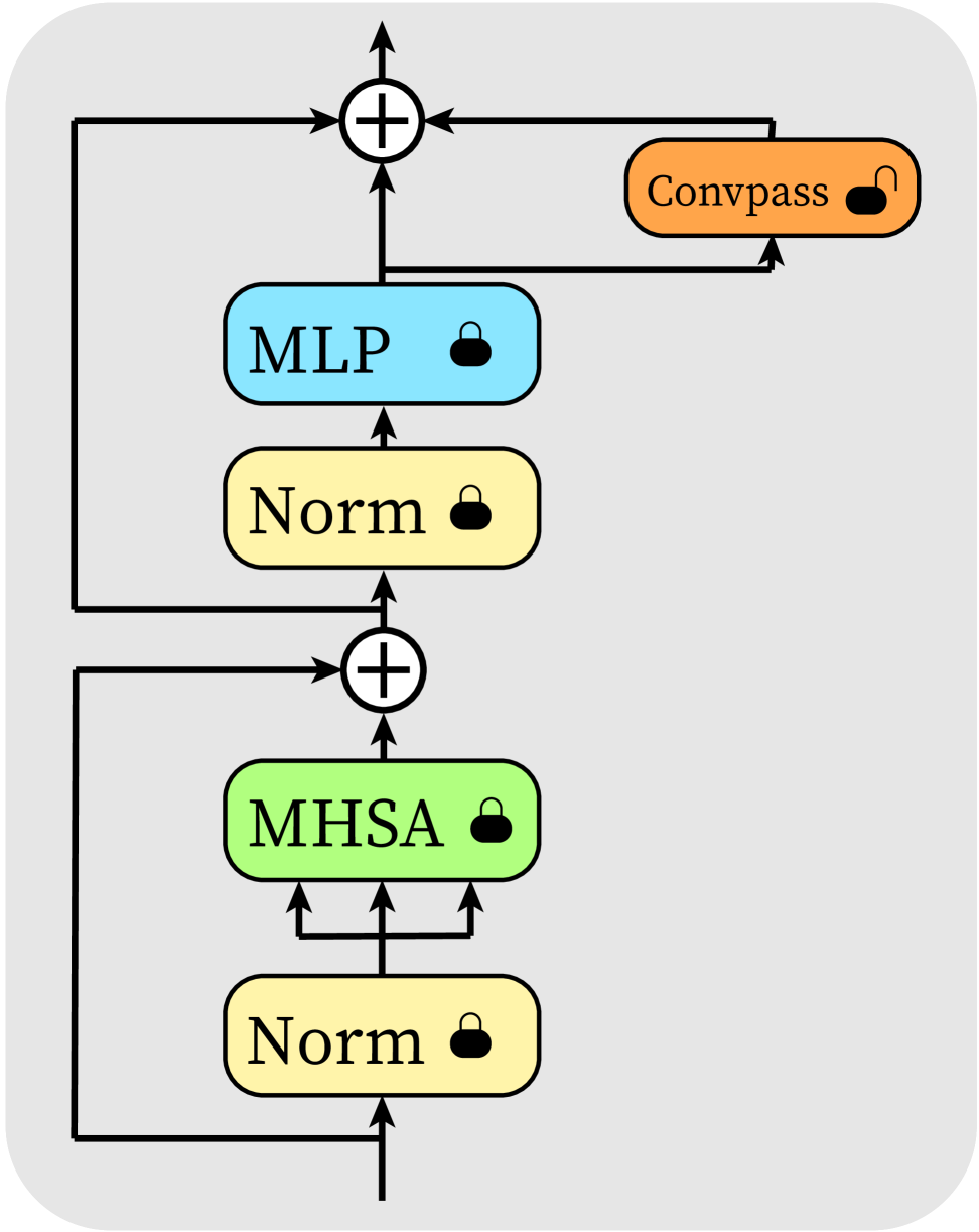
(c) Seq-Convpass${}_{\textit{mlp}}$

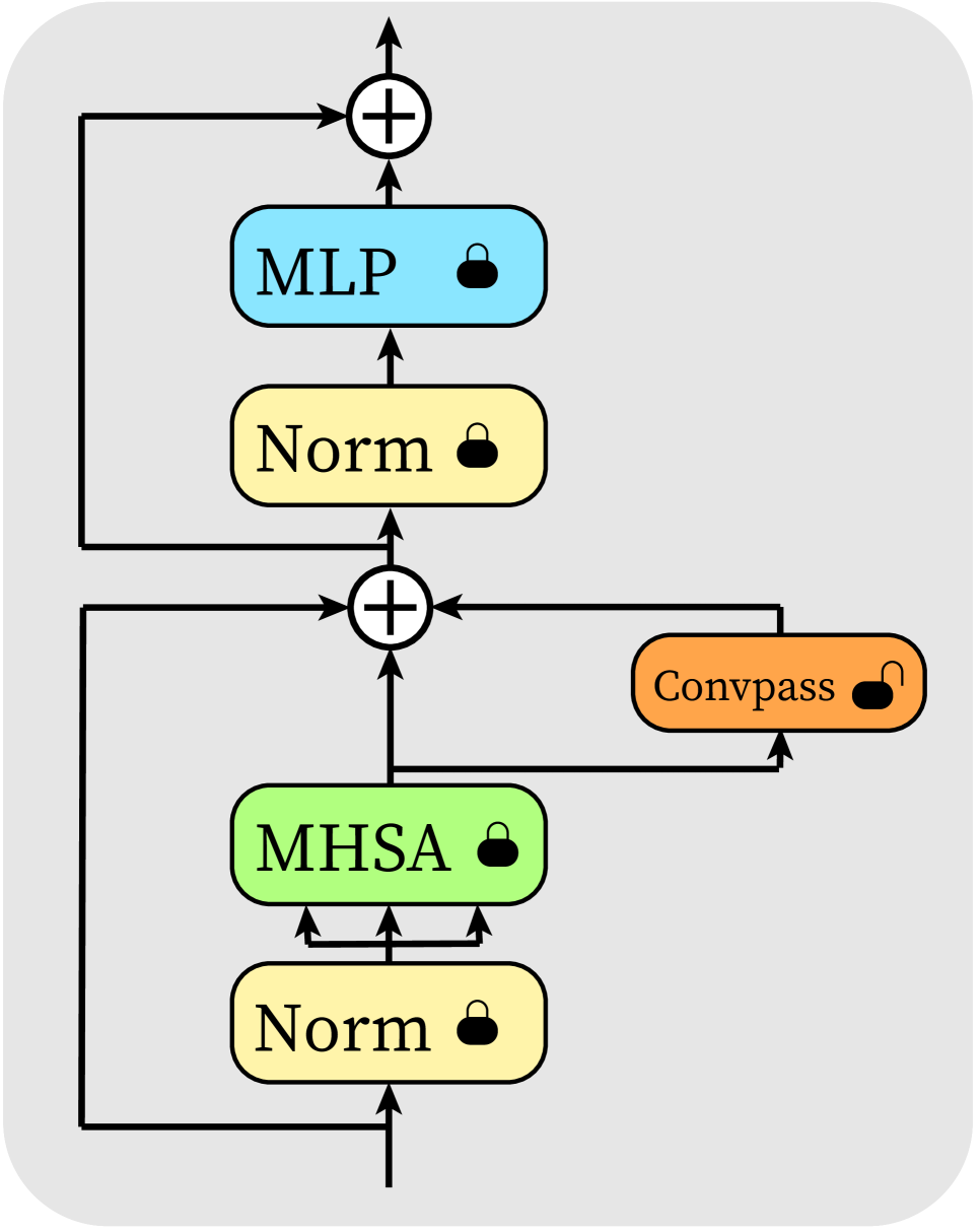
(d) Seq-Convpass${}_{\textit{attn}}$

Figure 6: Four ways to insert a Convpass module into ViT.

Moreover, we also apply Convpass to Swin. Similarly, Convpass modules bypass the W-MHSA/SW-MHSA/MLP blocks of Swin. As shown in Table 3, the advantage of Convpass over full finetuning still holds on Swin, but VPT is no longer competitive. This observation demonstrates that Convpass is a reliable PETL method performing constantly well on various backbone networks. From the comparison between Swin and ViT we also find that the improvement made by Convpass diminishes on Swin. This is also expected because the demand for supplementing visual inductive on Swin is not as pressing as on ViT.

Method	Avg.	Nat.	Spe.	Str.
Seq-Convpass${}_{\textit{mlp}}$	74.5	80.0	83.6	59.9
Seq-Convpass${}_{\textit{attn}}$	74.9	80.6	84.1	60.0
Convpass${}_{\textit{mlp}}$	75.4	80.3	84.5	61.2
Convpass${}_{\textit{attn}}$	75.8	81.2	84.7	61.5

Table 4: Results on VTAB-1K. We find that (i) parallel is superior to sequential, and (ii) alongside MHSA is superior to alongside MLP.

@MLP	@MHSA	Avg.	Nat.	Spe.	Str.
1$\times$1	1$\times$1	75.1	81.1	84.8	59.5
3$\times$3	1$\times$1	75.8	81.2	84.4	61.7
1$\times$1	3$\times$3	75.8	81.3	84.4	61.5
3$\times$3	3$\times$3	76.6	81.7	85.3	62.7

Table 5: Results on VTAB-1K. “1$\times$1 @MLP” means the 3$\times$3 convolutions in Convpass modules alongside the MLP blocks are replaced with 1$\times$1 convolutions. We find that vision-oriented is superior to language-oriented.

Where to Place the Convpass Modules

Our Convpass modules are parallel to the MHSA/MLP blocks, but there is another choice: insert the modules after the MHSA/MLP blocks in a sequential way like Adapter. To figure out what is the optimal way to place the Convpass modules, we consider four forms when only one Convpass module is inserted in each ViT layer , as illustrated in Figure 6. Convpass${}_{\textit{mlp}}$ and Convpass${}_{\textit{attn}}$ are parallel Convpass modules alongside the MLP and MHSA blocks, while Seq-Convpass${}_{\textit{mlp}}$ and Seq-Convpass${}_{\textit{attn}}$ follow the MLP and MHSA blocks, respectively.

As shown in Table 4, we evaluate these designs on VTAB-1K, and find the following. First, the parallel designs are better than their sequential counterparts. From Figure 2, we know that the sequential modules add longer paths to the model, which are relatively harder to optimize with a small amount of downstream data. On the contrary, the parallel Convpass serve as shortcuts for better gradient propagation, and introduce fully-convolutional ResNet-like paths that do not exist in sequential designs. Second, we also find that placing the Convpass modules beside/after MHSA blocks is better than beside/after MLP blocks. Since Convpass${}_{\textit{attn}}$ and Convpass${}_{\textit{mlp}}$ are the best two designs, our Convpass is composed of them, i.e., placing Convpass modules alongside both MHSA and MLP blocks in parallel.

Vision-Oriented vs. Language-Oriented

Finally, we conduct an ablation study on the vision-oriented idea. As shown in Table 5, we replace the 3$\times$3 convolutions in Convpass modules alongside the MLP and/or MHSA with 1$\times$1 convolutions, yielding four different designs. The bottom row is exactly Compass. Replacing the 3$\times$3 convolution in a Convpass module means the module will lose its capacity as a token mixer, degrading into a language-oriented adaptation module similar to Adapter.

The results show that, whether we replace the 3$\times$3 convolutions of Convpass modules alongside MLP or alongside MHSA, the performance on Natural, Specialized, and Structured tasks will all degrade. If all 3$\times$3 convolutions are replaced, the model will perform rather poorly on Structured. Since the Structured tasks are about obtaining the structure of a scene (e.g., object counting or 3D depth prediction), they fairly differ from the pretraining tasks (i.e., ImageNet classification) and require more modifications to the pretrained token mixer. Therefore, the Structured tasks are more complicated and the superiority of vision-oriented modules is highlighted. In summary, the language-oriented ablation models perform worse than the vision-oriented Convpass, supporting our standpoint.

5 Conclusion

In this paper, we point out that current PETL methods used in ViT lack inductive bias for visual tasks, which potentially degrades the performance on downstream finetuning. For this reason, we propose Convpass, a vision-oriented PETL method that employs trainable convolotional bypasses to adapt pretrained ViT to downstream tasks. Experimental results on VTAB-1K benchmark and few-shot learning show that Convpass outperforms other PETL methods and owns remarkable domain generalization property. Our simple but effective method reveals the importance of considering the characteristics of visual tasks when designing ViT-based PETL methods, which lights a promising direction for future work.

Appendix

A Datasets

See Table 6. Since the test set of ImageNet-1K has not been released, we report its validation results in our experiments.

	Dataset	# Classes	Train	Val	Test
VTAB-1K (Zhai et al. 2019)
Natural	CIFAR100 (Krizhevsky, Hinton et al. 2009)	100	800/1,000	200	10,000
	Caltech101 (Fei-Fei, Fergus, and Perona 2004)	102			6,084
	DTD (Cimpoi et al. 2014)	47			1,880
	Oxford-Flowers102 (Nilsback and Zisserman 2006)	102			6,149
	Oxford-Pets (Parkhi et al. 2012)	37			3,669
	SVHN (Netzer et al. 2011)	10			26,032
	Sun397 (Xiao et al. 2010)	397			21,750
Specialized	Patch Camelyon (Veeling et al. 2018)	2	800/1,000	200	32,768
	EuroSAT (Helber et al. 2019)	10			5,400
	Resisc45 (Cheng, Han, and Lu 2017)	45			6,300
	Retinopathy (Kaggle and EyePacs 2015)	5			42,670
Structured	Clevr/count (Johnson et al. 2017)	8	800/1,000	200	15,000
	Clevr/distance (Johnson et al. 2017)	6			15,000
	DMLab (Beattie et al. 2016)	6			22,735
	KITTI-Dist (Geiger et al. 2013)	4			711
	dSprites/location (Matthey et al. 2017)	16			73,728
	dSprites/orientation (Matthey et al. 2017)	16			73,728
	SmallNORB/azimuth (LeCun, Huang, and Bottou 2004)	18			12,150
	SmallNORB/elevation (LeCun, Huang, and Bottou 2004)	18			12,150
Few-shot learning
	Food-101 (Bossard, Guillaumin, and Gool 2014)	101	1/2/4/8/16 per class	20,200	30,300
	Stanford Cars (Krause et al. 2013)	196		1,635	8,041
	Oxford-Flowers102 (Nilsback and Zisserman 2006)	102		1,633	2,463
	FGVC-Aircraft (Maji et al. 2013b)	100		3,333	3,333
	Oxford-Pets (Parkhi et al. 2012)	37		736	3,669
Domain generalization
	ImageNet-1K (Deng et al. 2009)	1,000	16 per class	50,000	N/A
	ImageNet-V2 (Recht et al. 2019)	1,000	N/A	N/A	10,000
	ImageNet-Sketch (Wang et al. 2019)	1,000	N/A	N/A	50,889
	ImageNet-A (Hendrycks et al. 2021b)	200	N/A	N/A	7,500
	ImageNet-R (Hendrycks et al. 2021a)	200	N/A	N/A	30,000

Table 6: Statistics of used datasets.

B Experimental Details

B.1 Pretrained Backbones

See Table 7.

Model	Pretraining Dataset	Size (M)	Pretrained Weights
ViT-B/16 (Dosovitskiy et al. 2021)	ImageNet-21K	85.8	checkpoint
Swin-B (Liu et al. 2021b)	ImageNet-21K	86.7	checkpoint
ConvNeXt-B (Liu et al. 2022)	ImageNet-21K	87.6	checkpoint
CLIP ViT-B/16 (Radford et al. 2021)	WebImageText	85.8 (image encoder)	checkpoint

Table 7: Pretrained backbones.

B.2 Code Implementation

We use PyTorch to implement all experiments on NVIDIA RTX3090 GPUs. The models are implemented based on timm.

B.3 Data Augmentation

VTAB-1K

Following (Jia et al. 2022; Zhang, Zhou, and Liu 2022), we resize the images to $224\times 224$, and then normalize them with ImageNet’s mean and standard deviation.

Few-shot learning

Following (Zhang, Zhou, and Liu 2022), for training samples, we use color-jitter and RandAugmentation; for validation/test samples, we resize them to $256\times 256$, crop them to $224\times 224$ at the center, and then normalize them with ImageNet’s mean and standard deviation.

Domain generalization

Following (Zhou et al. 2022), for training samples, we randomly resize and crop them to $224\times 224$, and then implement random horizontal flip; for validation/test samples, we resize them to $224\times 224$. All samples are finally normalized with ImageNet’s mean and standard deviation.

B.4 Hyperparameters

$s$ is searched from {0.01, 0.1, 1, 10, 100}. See Table 8 for other hyperparameters.

	optimizer	batch size	learning rate	weight decay	# epochs	lr decay	# warm-up epochs
VTAB-1K	AdamW	64	1e-3	1e-4	100	cosine	10
Few-shot learning	AdamW	64	5e-3	1e-4	100	cosine	10
Domain generalization	AdamW	64	1e-5	0	50	cosine	0

Table 8: Hyperparameters.

B.5 Results of Adapter

We notice that it is reported by Jia et al. (2022) that Adapter significantly underperforms VPT. This is because their implementation uses zero-initialization for weights of both the two FC layers in Adapter, which blocks the backpropagation of gradient. Therefore, we follow Zhang, Zhou, and Liu (2022) using Xavier-initialization for weights and zero-initialization for biases, and report results that Adapter outperforms VPT.

References

- Ba, Kiros, and Hinton (2016) Ba, L. J.; Kiros, J. R.; and Hinton, G. E. 2016. Layer Normalization. CoRR, abs/1607.06450.
- Bao, Dong, and Wei (2022) Bao, H.; Dong, L.; and Wei, F. 2022. BEiT: BERT Pre-Training of Image Transformers. In ICLR.
- Beattie et al. (2016) Beattie, C.; Leibo, J. Z.; Teplyashin, D.; Ward, T.; Wainwright, M.; Küttler, H.; Lefrancq, A.; Green, S.; Valdés, V.; Sadik, A.; et al. 2016. Deepmind lab. CoRR, abs/1612.03801.
- Bossard, Guillaumin, and Gool (2014) Bossard, L.; Guillaumin, M.; and Gool, L. V. 2014. Food-101–mining discriminative components with random forests. In ECCV.
- Brown et al. (2020) Brown, T. B.; Mann, B.; Ryder, N.; Subbiah, M.; Kaplan, J.; Dhariwal, P.; Neelakantan, A.; Shyam, P.; Sastry, G.; Askell, A.; Agarwal, S.; Herbert-Voss, A.; Krueger, G.; Henighan, T.; Child, R.; Ramesh, A.; Ziegler, D. M.; Wu, J.; Winter, C.; Hesse, C.; Chen, M.; Sigler, E.; Litwin, M.; Gray, S.; Chess, B.; Clark, J.; Berner, C.; McCandlish, S.; Radford, A.; Sutskever, I.; and Amodei, D. 2020. Language Models are Few-Shot Learners. CoRR, abs/2005.14165.
- Chen et al. (2022) Chen, S.; Ge, C.; Tong, Z.; Wang, J.; Song, Y.; Wang, J.; and Luo, P. 2022. AdaptFormer: Adapting Vision Transformers for Scalable Visual Recognition. CoRR, abs/2205.13535.
- Cheng, Han, and Lu (2017) Cheng, G.; Han, J.; and Lu, X. 2017. Remote Sensing Image Scene Classification: Benchmark and State of the Art. Proc. IEEE.
- Cimpoi et al. (2014) Cimpoi, M.; Maji, S.; Kokkinos, I.; Mohamed, S.; ; and Vedaldi, A. 2014. Describing Textures in the Wild. In CVPR.
- Deng et al. (2009) Deng, J.; Dong, W.; Socher, R.; Li, L.-J.; Li, K.; and Fei-Fei, L. 2009. ImageNet: A large-scale hierarchical image database. In CVPR.
- Devlin et al. (2019) Devlin, J.; Chang, M.; Lee, K.; and Toutanova, K. 2019. BERT: Pre-training of Deep Bidirectional Transformers for Language Understanding. In NAACL-HLT.
- Dosovitskiy et al. (2021) Dosovitskiy, A.; Beyer, L.; Kolesnikov, A.; Weissenborn, D.; Zhai, X.; Unterthiner, T.; Dehghani, M.; Minderer, M.; Heigold, G.; Gelly, S.; Uszkoreit, J.; and Houlsby, N. 2021. An Image is Worth 16x16 Words: Transformers for Image Recognition at Scale. In ICLR.
- Fei-Fei, Fergus, and Perona (2004) Fei-Fei, L.; Fergus, R.; and Perona, P. 2004. Learning generative visual models from few training examples: An incremental bayesian approach tested on 101 object categories. In CVPR workshop.
- Geiger et al. (2013) Geiger, A.; Lenz, P.; Stiller, C.; and Urtasun, R. 2013. Vision meets robotics: The kitti dataset. The International Journal of Robotics Research.
- He et al. (2022a) He, J.; Zhou, C.; Ma, X.; Berg-Kirkpatrick, T.; and Neubig, G. 2022a. Towards a Unified View of Parameter-Efficient Transfer Learning. In ICLR.
- He et al. (2022b) He, K.; Chen, X.; Xie, S.; Li, Y.; Dollár, P.; and Girshick, R. B. 2022b. Masked Autoencoders Are Scalable Vision Learners. In CVPR.
- He et al. (2016) He, K.; Zhang, X.; Ren, S.; and Sun, J. 2016. Deep Residual Learning for Image Recognition. In CVPR.
- Helber et al. (2019) Helber, P.; Bischke, B.; Dengel, A.; and Borth, D. 2019. Eurosat: A novel dataset and deep learning benchmark for land use and land cover classification. IEEE Journal of Selected Topics in Applied Earth Observations and Remote Sensing.
- Hendrycks et al. (2021a) Hendrycks, D.; Basart, S.; Mu, N.; Kadavath, S.; Wang, F.; Dorundo, E.; Desai, R.; Zhu, T.; Parajuli, S.; Guo, M.; Song, D.; Steinhardt, J.; and Gilmer, J. 2021a. The Many Faces of Robustness: A Critical Analysis of Out-of-Distribution Generalization. In ICCV.
- Hendrycks et al. (2021b) Hendrycks, D.; Zhao, K.; Basart, S.; Steinhardt, J.; and Song, D. 2021b. Natural Adversarial Examples. In CVPR.
- Houlsby et al. (2019) Houlsby, N.; Giurgiu, A.; Jastrzebski, S.; Morrone, B.; de Laroussilhe, Q.; Gesmundo, A.; Attariyan, M.; and Gelly, S. 2019. Parameter-Efficient Transfer Learning for NLP. In ICML.
- Hu et al. (2022) Hu, E. J.; yelong shen; Wallis, P.; Allen-Zhu, Z.; Li, Y.; Wang, S.; Wang, L.; and Chen, W. 2022. LoRA: Low-Rank Adaptation of Large Language Models. In ICLR.
- Jia et al. (2022) Jia, M.; Tang, L.; Chen, B.; Cardie, C.; Belongie, S. J.; Hariharan, B.; and Lim, S. 2022. Visual Prompt Tuning. In ECCV.
- Johnson et al. (2017) Johnson, J.; Hariharan, B.; Van Der Maaten, L.; Fei-Fei, L.; Lawrence Zitnick, C.; and Girshick, R. 2017. Clevr: A diagnostic dataset for compositional language and elementary visual reasoning. In CVPR.
- Kaggle and EyePacs (2015) Kaggle; and EyePacs. 2015. Kaggle diabetic retinopathy detection.
- Kolesnikov et al. (2020) Kolesnikov, A.; Beyer, L.; Zhai, X.; Puigcerver, J.; Yung, J.; Gelly, S.; and Houlsby, N. 2020. Big Transfer (BiT): General Visual Representation Learning. In ECCV.
- Krause et al. (2013) Krause, J.; Stark, M.; Deng, J.; and Fei-Fei, L. 2013. 3d object representations for fine-grained categorization. In CVPR workshops.
- Krizhevsky, Hinton et al. (2009) Krizhevsky, A.; Hinton, G.; et al. 2009. Learning multiple layers of features from tiny images.
- LeCun, Huang, and Bottou (2004) LeCun, Y.; Huang, F. J.; and Bottou, L. 2004. Learning methods for generic object recognition with invariance to pose and lighting. In CVPR.
- Li and Liang (2021) Li, X. L.; and Liang, P. 2021. Prefix-Tuning: Optimizing Continuous Prompts for Generation. In ACL/IJCNLP.
- Liu et al. (2021a) Liu, X.; Ji, K.; Fu, Y.; Du, Z.; Yang, Z.; and Tang, J. 2021a. P-Tuning v2: Prompt Tuning Can Be Comparable to Fine-tuning Universally Across Scales and Tasks. CoRR, abs/2110.07602.
- Liu et al. (2021b) Liu, Z.; Lin, Y.; Cao, Y.; Hu, H.; Wei, Y.; Zhang, Z.; Lin, S.; and Guo, B. 2021b. Swin Transformer: Hierarchical Vision Transformer using Shifted Windows. In ICCV.
- Liu et al. (2022) Liu, Z.; Mao, H.; Wu, C.; Feichtenhofer, C.; Darrell, T.; and Xie, S. 2022. A ConvNet for the 2020s. In CVPR.
- Maji et al. (2013a) Maji, S.; Rahtu, E.; Kannala, J.; Blaschko, M.; and Vedaldi, A. 2013a. Fine-grained visual classification of aircraft. CoRR, abs/1306.5151.
- Maji et al. (2013b) Maji, S.; Rahtu, E.; Kannala, J.; Blaschko, M. B.; and Vedaldi, A. 2013b. Fine-Grained Visual Classification of Aircraft. CoRR, abs/1306.5151.
- Matthey et al. (2017) Matthey, L.; Higgins, I.; Hassabis, D.; and Lerchner, A. 2017. dsprites: Disentanglement testing sprites dataset.
- Netzer et al. (2011) Netzer, Y.; Wang, T.; Coates, A.; Bissacco, A.; Wu, B.; and Ng, A. Y. 2011. Reading digits in natural images with unsupervised feature learning.
- Nilsback and Zisserman (2006) Nilsback, M.-E.; and Zisserman, A. 2006. A visual vocabulary for flower classification. In CVPR.
- Parkhi et al. (2012) Parkhi, O. M.; Vedaldi, A.; Zisserman, A.; and Jawahar, C. 2012. Cats and dogs. In CVPR.
- Pfeiffer et al. (2021) Pfeiffer, J.; Kamath, A.; Rücklé, A.; Cho, K.; and Gurevych, I. 2021. AdapterFusion: Non-Destructive Task Composition for Transfer Learning. In EACL.
- Radford et al. (2021) Radford, A.; Kim, J. W.; Hallacy, C.; Ramesh, A.; Goh, G.; Agarwal, S.; Sastry, G.; Askell, A.; Mishkin, P.; Clark, J.; Krueger, G.; and Sutskever, I. 2021. Learning Transferable Visual Models From Natural Language Supervision. In ICML, Proceedings of Machine Learning Research.
- Raffel et al. (2020) Raffel, C.; Shazeer, N.; Roberts, A.; Lee, K.; Narang, S.; Matena, M.; Zhou, Y.; Li, W.; and Liu, P. J. 2020. Exploring the Limits of Transfer Learning with a Unified Text-to-Text Transformer. J. Mach. Learn. Res., 21: 140:1–140:67.
- Recht et al. (2019) Recht, B.; Roelofs, R.; Schmidt, L.; and Shankar, V. 2019. Do ImageNet Classifiers Generalize to ImageNet? In ICML.
- Vaswani et al. (2017) Vaswani, A.; Shazeer, N.; Parmar, N.; Uszkoreit, J.; Jones, L.; Gomez, A. N.; Kaiser, L.; and Polosukhin, I. 2017. Attention is All you Need. In NIPS.
- Veeling et al. (2018) Veeling, B. S.; Linmans, J.; Winkens, J.; Cohen, T.; and Welling, M. 2018. Rotation Equivariant CNNs for Digital Pathology. CoRR, abs/1806.03962.
- Veit, Wilber, and Belongie (2016) Veit, A.; Wilber, M. J.; and Belongie, S. J. 2016. Residual Networks Behave Like Ensembles of Relatively Shallow Networks. In NIPS.
- Wang et al. (2019) Wang, H.; Ge, S.; Lipton, Z. C.; and Xing, E. P. 2019. Learning Robust Global Representations by Penalizing Local Predictive Power. In NeurIPS.
- Wang et al. (2021) Wang, W.; Bao, H.; Dong, L.; and Wei, F. 2021. VLMo: Unified Vision-Language Pre-Training with Mixture-of-Modality-Experts. CoRR, abs/2111.02358.
- Wu et al. (2021) Wu, H.; Xiao, B.; Codella, N.; Liu, M.; Dai, X.; Yuan, L.; and Zhang, L. 2021. CvT: Introducing Convolutions to Vision Transformers. In ICCV.
- Xiao et al. (2010) Xiao, J.; Hays, J.; Ehinger, K. A.; Oliva, A.; and Torralba, A. 2010. Sun database: Large-scale scene recognition from abbey to zoo. In CVPR.
- Yu et al. (2022) Yu, J.; Wang, Z.; Vasudevan, V.; Yeung, L.; Seyedhosseini, M.; and Wu, Y. 2022. CoCa: Contrastive Captioners are Image-Text Foundation Models. CoRR, abs/2205.01917.
- Zaken, Goldberg, and Ravfogel (2022) Zaken, E. B.; Goldberg, Y.; and Ravfogel, S. 2022. BitFit: Simple Parameter-efficient Fine-tuning for Transformer-based Masked Language-models. In Muresan, S.; Nakov, P.; and Villavicencio, A., eds., ACL.
- Zhai et al. (2022) Zhai, X.; Kolesnikov, A.; Houlsby, N.; and Beyer, L. 2022. Scaling vision transformers. In CVPR.
- Zhai et al. (2019) Zhai, X.; Puigcerver, J.; Kolesnikov, A.; Ruyssen, P.; Riquelme, C.; Lucic, M.; Djolonga, J.; Pinto, A. S.; Neumann, M.; Dosovitskiy, A.; Beyer, L.; Bachem, O.; Tschannen, M.; Michalski, M.; Bousquet, O.; Gelly, S.; and Houlsby, N. 2019. The Visual Task Adaptation Benchmark. CoRR, abs/1910.04867.
- Zhang et al. (2020) Zhang, J. O.; Sax, A.; Zamir, A. R.; Guibas, L. J.; and Malik, J. 2020. Side-Tuning: A Baseline for Network Adaptation via Additive Side Networks. In Vedaldi, A.; Bischof, H.; Brox, T.; and Frahm, J., eds., ECCV.
- Zhang et al. (2022) Zhang, R.; Fang, R.; Gao, P.; Zhang, W.; Li, K.; Dai, J.; Qiao, Y.; and Li, H. 2022. Tip-Adapter: Training-free Adaption of CLIP for Few-shot Classification. In ECCV.
- Zhang, Zhou, and Liu (2022) Zhang, Y.; Zhou, K.; and Liu, Z. 2022. Neural Prompt Search. CoRR, abs/2206.04673.
- Zhou et al. (2021) Zhou, K.; Yang, J.; Loy, C. C.; and Liu, Z. 2021. Learning to Prompt for Vision-Language Models. CoRR, abs/2109.01134.
- Zhou et al. (2022) Zhou, K.; Yang, J.; Loy, C. C.; and Liu, Z. 2022. Conditional Prompt Learning for Vision-Language Models. In CVPR.