Quark and gluon two-loop beam functions for leading-jet $p_{T}$ and slicing at NNLO

Abstract

We compute the complete set of two-loop beam functions for the transverse momentum distribution of the leading jet produced in association with an arbitrary colour-singlet system. Our results constitute the last missing ingredient for the calculation of the jet-vetoed cross section at small veto scales at the next-to-next-to-leading order, as well as an important ingredient for its resummation to next-to-next-to-next-to-leading logarithmic order. Our calculation is performed in the soft-collinear effective theory framework with a suitable regularisation of the rapidity divergences occurring in the phase-space integrals. We discuss the occurrence of soft-collinear mixing terms that might violate the factorisation theorem, and demonstrate that they vanish at two loops in the exponential rapidity regularisation scheme when performing a multipole expansion of the measurement function. As in our recent computation of the two-loop soft function, we present the results as a Laurent expansion in the jet radius $R$. We provide analytic expressions for all flavour channels in $x$ space with the exception of a set of $R$-independent non-logarithmic terms that are given as numerical grids. We also perform a fully numerical calculation with exact $R$ dependence, and find that it agrees with our analytic expansion at the permyriad level or better. Our calculation allows us to define a next-to-next-to-leading order slicing method using the leading-jet $p_{T}$ as a slicing variable. As a check of our results, we carry out a calculation of the Higgs and $Z$ boson total production cross sections at the next-to-next-to-leading order in QCD.

1 Introduction

Precision measurements at hadron colliders often rely on jet vetoes to reduce the impact of background due to QCD radiation. This is done by rejecting events containing jets with a transverse momentum exceeding some cutoff value $p_{T}^{\rm veto}$ that is often much smaller than the large momentum transfer of the hard scattering process $Q$. This strategy finds common applications in the field of Higgs physics, as well as in a number of electro-weak and QCD measurements at the Large Hadron Collider (LHC), and has therefore motivated a large number of studies Banfi:2012yh ; Becher:2012qa ; Banfi:2012jm ; Banfi:2013eda ; Becher:2013xia ; Stewart:2013faa ; Banfi:2015pju ; Becher:2014aya ; Moult:2014pja ; Jaiswal:2014yba ; Monni:2014zra ; Wang:2015mvz ; Dawson:2016ysj ; Monni:2019yyr ; Kallweit:2020gva . For instance, the state-of-the-art prediction for the jet-vetoed Higgs production cross section involves the resummation of the large logarithms $\ln(p_{T}^{\rm veto}/Q)$ up to next-to-next-to-leading logarithmic (NNLL) order Banfi:2012jm ; Banfi:2013eda ; Becher:2013xia ; Stewart:2013faa matched to fixed order calculations up to next-to-next-to-next-to-leading order (N³LO) Banfi:2015pju . The above NNLL calculations also include a numerical extraction of the ${\cal O}(\alpha_{s}^{2})$ non-logarithmic terms relative to the Born (often referred to as NNLL^′) from fixed-order calculations. In this article, we will complete the direct calculation of such constant terms in view of pushing the resummation accuracy to N³LL, which is demanded by the outstanding experimental precision foreseen at the LHC in the coming years.

Specifically, we consider the calculation of the two-loop beam functions entering the factorisation and resummation of the jet-vetoed cross section. Beam functions describe the dynamics of radiation collinear to the beam direction in high-energy hadron collisions. Together with our recent calculation of the two-loop soft function in Ref. Abreu:2022sdc , the results presented here constitute the last missing ingredient for the calculation of the jet-vetoed cross section at small value of the veto scale (i.e., up to power corrections in $p_{T}^{\rm veto}/Q$) at the next-to-next-to-leading order (NNLO), and an important step towards the resummation of the leading-jet transverse momentum distribution (and the related jet-vetoed cross section) at N³LL order. Moreover, our results allow us to construct a slicing method for NNLO calculations in QCD using the leading-jet transverse momentum as a slicing variable.

We work in the framework of soft-collinear effective field theory (SCET) Bauer:2000yr ; Bauer:2001yt ; Bauer:2002nz ; Beneke:2002ph ; Beneke:2002ni . More specifically, the jet-veto cross section belongs to the class of SCET_II problems, which are affected by the so-called factorisation (or collinear) anomaly BenekeFA ; Becher:2010tm , connected to the presence of rapidity divergences in the ingredients of the factorisation theorem. Such divergences are not regulated by the standard dimensional regularisation scheme and therefore an additional (rapidity) regulator must be introduced. Here we use the exponential regularisation scheme Li:2016axz , consistently with our recent calculation of the two-loop soft function Abreu:2022sdc .

The validity of SCET factorisation for this observable at arbitrary logarithmic order has been the subject of debate in the literature Tackmann:2012bt ; Stewart:2013faa ; Becher:2013xia . Indeed, particular attention must be paid to the presence of soft-collinear mixing terms that might violate the factorisation theorem for this observable. While some groups Tackmann:2012bt ; Stewart:2013faa suggest that the SCET factorisation would be broken already at the next-to-next-to-leading logarithmic (NNLL) order, the authors of Ref. Becher:2013xia present an argument as to why such terms should cancel if one performs a consistent multipole expansion of the measurement functions. Following the observation of Ref. Becher:2013xia , we explicitly show here that within the exponential regularisation scheme such a multipole expansion of the jet-clustering measurement function leads to the cancellation of the factorisation breaking terms, in the regime in which the jet radius $R$ is treated as an $\mathcal{O}(1)$ parameter. This explicitly confirms the validity of the factorisation theorem at NNLO, and constitutes an important step towards the resummation at the N³LL order.

The article is organised as follows. In section 2, we review the factorisation theorem for the production of a colour-singlet with a veto on the transverse momentum of the leading jet and we discuss the definition of the beam functions in the presence of a rapidity regulator. Section 3 contains a discussion of our analytic computation of the two-loop beam functions as a small-$R$ expansion, as well as the details related to the zero-bin subtraction and the cancellation of the soft-collinear mixing terms. Section 4 reviews our numerical calculation of the beam functions that retains the full-$R$ dependence, and compares the results obtained by the analytic and numerical computations, finding good agreement between the two. Finally, in section 5 we construct a phase-space slicing scheme based on the leading-jet transverse momentum for fully differential NNLO calculations of the production of colour-singlet systems. We test the scheme, and our results, by calculating the NNLO total cross section for Higgs and $Z$ boson production at the LHC. Finally, our conclusions are given in section 6.

2 Factorisation of leading-jet transverse momentum in SCET

We begin by recalling the factorisation theorem for the jet-vetoed cross-section. We consider the production of an arbitrary colour-singlet system of total invariant mass $Q$ in proton-proton collisions. The cross section, differential in the system’s kinematics ${d}\Phi_{\rm Born}$ and with a veto on the transverse momentum of the leading jet $p_{T}^{\rm jet}<p_{T}^{\rm veto}$, factorises in the limit $p_{T}^{\rm veto}\ll Q$ as (${d}\sigma(p_{T}^{\rm veto})\equiv\frac{{d}\sigma(p_{T}^{\rm veto})}{{d}\Phi_{\rm Born}}$) Becher:2012qa ; Stewart:2013faa ; Becher:2013xia

$${d}\sigma(p_{T}^{\rm veto}) \equiv\sum_{F=q,g}|{\cal A}^{F}_{\rm Born}|^{2}\,{\cal H}^{F}(Q;\mu)$$

$$\times\,{\cal B}^{F}_{n}(x_{1},Q,p_{T}^{\rm veto},R^{2};\mu,\nu)\,{\cal B}^{F}_{\bar{n}}(x_{2},Q,p_{T}^{\rm veto},R^{2};\mu,\nu)\,{\cal S}^{F}(p_{T}^{\rm veto},R^{2};\mu,\nu)\,,$$ (1)

where ${\cal A}^{F}_{\rm Born}$ is the Born amplitude for the production of the colour-singlet system, and $\mu$ and $\nu$ denote the renormalisation and rapidity scales, respectively. The index $F$ indicates the flavour configuration of the initial state, i.e. either $q\bar{q}$ ($F=q$) or $gg$ ($F=g$), and for simplicity we will drop it from now on when referring to the ingredients of the factorisation theorem (2). The hard function ${\cal H}$ describes the dynamics at the hard scale, i.e. with virtuality $\mu\sim Q$. This scale is integrated-out in the SCET construction. Therefore, the hard function contains purely virtual contributions, and it is defined as the squared matching coefficient of the leading-power two-jet SCET current, i.e.

$${\cal H}^{F}(Q;\mu)=|{\cal C}^{F}(Q;\mu)|^{2}\,.$$ (2)

The soft function ${\cal S}$ describes the dynamics of soft radiation off the initial-state partons and is defined as a matrix element of soft Wilson lines. Lastly, the beam functions are denoted by ${\cal B}_{n}$ and ${\cal B}_{\bar{n}}$. Their two-loop calculation is the main focus of this paper. They are defined by matrix elements of collinear fields in SCET and describe the (anti-)collinear dynamics of radiation along the light-cone directions $n^{\mu}$ and ${\bar{n}}^{\mu}$ of the beams.

Within the SCET formalism, the resummation of the logarithms $\ln p_{T}^{\rm veto}/Q$ appearing in Eq. (2) is achieved by evolving each of the functions in the factorisation theorem from their canonical scales to two common $\mu$, $\nu$ scales. The hard matching coefficient obeys the renormalisation group equation (RGE)

$$\frac{d}{d\ln\mu}\ln{\cal C}^{F}(Q;\mu)=\Gamma_{\rm cusp}^{F}(\alpha_{s}(\mu))\ln\frac{-Q^{2}}{\mu^{2}}+\gamma_{H}^{F}(\alpha_{s}(\mu))\,,$$ (3)

where $\Gamma_{\rm cusp}^{F}$ and $\gamma_{H}^{F}$ are the cusp and hard anomalous dimensions of the quark ($F=q$) or gluon ($F=g$) form factors, renormalised in the $\overline{\rm MS}$ scheme. The hard function’s canonical scale is the hard scale $\mu=Q$. The beam functions ${\cal B}_{i}$ depend, in addition to the renormalisation scale $\mu$, on the rapidity regularisation scale $\nu$. They satisfy a system of coupled evolution equations (see e.g. Refs. Becher:2013xia ; Stewart:2013faa ). The RGE is given by

$$\frac{d}{d\ln\mu}\ln{\cal B}^{F}_{i}(x,Q,p_{T}^{\rm veto},R^{2};\mu,\nu)=2\,\Gamma_{\rm cusp}^{F}(\alpha_{s}(\mu))\ln\frac{\nu}{Q}+\gamma_{B}^{F}(\alpha_{s}(\mu))\,,$$ (4)

and the rapidity evolution equation reads

$$\frac{d}{d\ln\nu}\ln{\cal B}^{F}_{i}(x,Q,p_{T}^{\rm veto},R^{2};\mu,\nu)=2\int_{p_{T}^{\rm veto}}^{\mu}\frac{d\mu^{\prime}}{\mu^{\prime}}\Gamma_{\rm cusp}^{F}(\alpha_{s}(\mu^{\prime}))-\frac{1}{2}\gamma_{\nu}^{F}(p_{T}^{\rm veto},R^{2})\,,$$ (5)

where $\gamma_{\nu}^{F}$ denotes the observable-dependent rapidity anomalous dimension. The boundary condition for the $\{\mu,\nu\}$ evolution is set at the canonical scales $\mu=p_{T}^{\rm veto}$ and $\nu=Q$. Finally, the evolution equations for the soft function read

$$\frac{d}{d\ln\mu}\ln{\cal S}^{F}(p_{T}^{\rm veto},R^{2};\mu,\nu)= 4\,\Gamma_{\rm cusp}^{F}(\alpha_{s}(\mu))\ln\frac{\mu}{\nu}+\gamma_{S}^{F}(\alpha_{s}(\mu))\,,$$

$$\frac{d}{d\ln\nu}\ln{\cal S}^{F}(p_{T}^{\rm veto},R^{2};\mu,\nu)= -4\int_{p_{T}^{\rm veto}}^{\mu}\frac{d\mu^{\prime}}{\mu^{\prime}}\Gamma_{\rm cusp}^{F}(\alpha_{s}(\mu^{\prime}))+\gamma_{\nu}^{F}(p_{T}^{\rm veto},R^{2})\,,$$ (6)

with canonical scales $\mu=\nu=p_{T}^{\rm veto}$. The dependence on the rapidity anomalous dimension cancels between the evolution of the soft and beam functions in the framework of the rapidity renormalisation group Chiu:2011qc ; Chiu:2012ir . The soft ($\gamma_{S}^{F}$) and collinear ($\gamma_{B}^{F}$) anomalous dimensions are related to the hard anomalous dimension $\gamma_{H}^{F}$ by the invariance of the physical cross section under a change of the renormalisation scale, that is

$$2\gamma_{H}^{F}+\gamma_{S}^{F}+2\gamma_{B}^{F}=0\,.$$ (7)

The resummation of the jet-vetoed cross section at N^kLL requires the cusp anomalous dimension $\Gamma_{\rm cusp}^{F}$ up to $k+1$ loops, and the anomalous dimensions $\gamma_{H}^{F}$, $\gamma_{S}^{F}$, $\gamma_{B}^{F}$, $\gamma_{\nu}^{F}$ up to $k$ loops. The boundary conditions (non-logarithmic terms) of the evolution equations need to be known up to $k-1$ loops. Achieving $\rm N^{3}LL$ accuracy for the jet-vetoed cross section requires the knowledge of the non-logarithmic terms in ${\cal C}(Q;\mu)$ at two loops, which is given by the QCD on-shell form-factor Becher:2006nr and has been known for a long time Matsuura:1987wt ; Gehrmann:2005pd . The two loop computation of the ${\cal S}$ function was presented in our earlier article Abreu:2022sdc . Below, we focus on the evaluation of the two-loop beam functions. While the two-loop anomalous dimensions are known, the non-logarithmic terms are computed here for the first time. Moreover, since the anomalous dimensions featuring in Eq. (7) are known up to three loops Moch:2004pa ; Gehrmann:2010ue ; Li:2014afw , with the results presented in this work, the only missing ingredient for the N³LL computation is the three-loop rapidity anomalous dimension $\gamma_{\nu}^{F}$.

2.1 The beam functions

The quark and gluon beam functions are defined as matrix elements of non-local collinear operators between the proton states $\left|P(p)\right\rangle$ carrying large momentum $p$. Specifically, we have Becher:2012qa ; Stewart:2013faa ; Becher:2013xia

$${\cal B}_{n}^{q}(x,Q,p_{T}^{\rm veto},R^{2};\mu,\nu) =\frac{1}{2\pi}\int dte^{-ixt\bar{n}\cdot p}\big{\langle}P(p)\big{|}\overline{\chi}_{n}(t\bar{n})\,\frac{\not{\bar{n}}}{2}\,{\mathbb{M}}(p_{T}^{\rm veto},R^{2})\,\chi_{n}(0)\big{|}P(p)\big{\rangle}\,,$$ (8)

$${\cal B}_{n}^{g}(x,Q,p_{T}^{\rm veto},R^{2};\mu,\nu) =-\frac{x\bar{n}\cdot p}{2\pi}\int dte^{-ixt\bar{n}\cdot p}\big{\langle}P(p)\big{|}\mathcal{A}^{\mu,a}_{\perp}(t\bar{n})\,{\mathbb{M}}(p_{T}^{\rm veto},R^{2})\,\mathcal{A}_{\perp,\mu}^{a}(0)\big{|}P(p)\big{\rangle}\,,$$

where the collinear-gauge invariant collinear building blocks are defined in terms of the fields

$$\chi(x)=W^{\dagger}\xi(x),\qquad\mathcal{A}^{\mu,A}_{\perp}=2{\rm tr}\left[W^{\dagger}\left[iD^{\mu}_{\perp}W\right](x)t^{A}\right]\,.$$ (9)

Here $\xi(x)$ is the collinear quark field and $D^{\mu}_{\perp}$ is the covariant $\perp$ collinear derivative. Gauge invariance is achieved by introducing the collinear Wilson line $W(x)$ defined as

$$W(x)=\mathcal{P}\exp\left[ig\int_{-\infty}^{0}ds\,\bar{n}A(x+s\bar{n})\right]\,.$$ (10)

The operator ${\mathbb{M}}(p_{T}^{\rm veto},R^{2})$ acts on a given state of $X_{c}$ collinear particles $|X_{c}\rangle$ by applying a veto on the final-state jets of radius $R$ such that $p_{T}^{\rm jet_{i}}<p_{T}^{\rm veto}$

$${\mathbb{M}}(p_{T}^{\rm veto},R^{2})|X_{c}\rangle=\mathcal{M}(p_{T}^{\rm veto},R^{2})|X_{c}\rangle\,,$$ (11)

with the phase space constraint $\mathcal{M}(p_{T}^{\rm veto},R^{2})$ being

$$\mathcal{M}(p_{T}^{\rm veto},R^{2})=\Theta(p_{T}^{\rm veto}-\max\{p_{T}^{\rm jet_{i}}\})\Theta_{\rm cluster}(R^{2})\,.$$ (12)

Here $\max\{p_{T}^{\rm jet_{i}}\}$ is the transverse momentum of the hardest jet, where jets are defined in the $E$ recombination scheme Cacciari:2011ma . The constraint $\Theta_{\rm cluster}(R^{2})$ is the generic clustering condition on the $X_{c}$ collinear final state particles, defined for a $k_{T}$-class of jet algorithms Cacciari:2008gp with jet distance measures

$$d_{ij}=\min\{k_{\perp i}^{2p},k_{\perp j}^{2p}\}\left[(\Delta\eta_{ij})^{2}+(\Delta\phi_{ij})^{2}\right]\,,\quad d_{iB}=k_{\perp i}^{2p}\,.$$ (13)

Specific choices of the parameter $p$ correspond to the anti-$k_{T}$ Cacciari:2008gp algorithm ($p=-1$), the Cambridge-Aachen Dokshitzer:1997in ; Wobisch:1998wt algorithm ($p=0$), and the $k_{T}$ Catani:1993hr algorithm ($p=1$). The results obtained in this article are valid for any of these choices. In Eq. (13), $k_{\perp i}$ is the transverse momentum of particle $i$ with respect to the beam direction, and $\Delta\eta_{ij}$ and $\Delta\phi_{ij}$ are the relative rapidity and azimuthal angle between particles $i$ and $j$, respectively. The particles are clustered sequentially with respect to the above distance measure, as specified by the clustering condition $\Theta_{\rm cluster}(R^{2})$.

Since the definition (8) involves matrix elements between proton states, the beam functions are in general non-perturbative objects. However, for $p_{T}^{\rm veto}\gg\Lambda_{\rm QCD}$, it is possible to perturbatively match them onto the standard parton distribution functions (PDFs) $f_{F/P}(x,\mu)$ as follows Becher:2012qa ; Stewart:2013faa ; Becher:2013xia ,

$${\cal B}_{F}(x,Q,p_{T}^{\rm veto},R^{2};\mu,\nu)=\sum_{F^{\prime}}\int_{x}^{1}\frac{dz}{z}I_{FF^{\prime}}(z,Q,p_{T}^{\rm veto},R^{2};\mu,\nu)f_{F^{\prime}/P}(x/z,\mu)+\mathcal{O}\left(\frac{\Lambda_{\rm QCD}}{p_{T}^{\rm veto}}\right)\,,$$ (14)

where the standard proton PDFs are defined as

$$f_{q/P}(x,\mu) =\frac{1}{2\pi}\int dte^{-ixt\bar{n}\cdot p}\big{\langle}P(p)\big{|}\overline{\chi}_{n}(t\bar{n})\,\frac{\not{\bar{n}}}{2}\,\chi_{n}(0)\big{|}P(p)\big{\rangle}\,,$$ (15)

$$f_{g/P}(x,\mu) =-\frac{x\bar{n}\cdot p}{2\pi}\int dte^{-ixt\bar{n}\cdot p}\big{\langle}P(p)\big{|}\mathcal{A}^{\mu,a}_{\perp}(t\bar{n})\,\mathcal{A}_{\perp,\mu}^{a}(0)\big{|}P(p)\big{\rangle}\,,$$

for the quark and the gluon, respectively.

The perturbative matching kernels $I_{FF^{\prime}}(z,Q,p_{T}^{\rm veto},R^{2};\mu,\nu)$ are short-distance Wilson coefficients, whose computation is the focus of this article. At the LO, the collinear partons do not radiate and we have $I_{FF^{\prime}}(z,Q,p_{T}^{\rm veto},R^{2};\mu,\nu)=\delta_{FF^{\prime}}\delta(1-z)$. The computation of radiative corrections to this relation up to the two-loop order will be the subject of Section 3.

The formal definition of the matching in Eq. (14) requires splitting the generic collinear fields into the perturbative collinear modes with the virtuality of the order of $p_{T}^{\rm veto}$ and the PDF-collinear modes with virtuality $\Lambda_{\rm QCD}$. The non-perturbative PDFs are then defined in terms of the matrix elements of the PDF-collinear modes only, while the perturbative collinear modes are integrated out from the theory. This distinction can often be ignored in practice at the leading power in SCET. Hence, in the rest of this article, we will refer to both types of collinear fields as simply collinear modes.

Even though Eq. (14) is written as an identity relating specific matrix elements, it represents an operatorial identity, which does not depend on the specific choice of the external states. Thus, to compute the matching kernels we can replace the external proton states by perturbative partonic states. With this replacement, the bare partonic PDF for finding a parton $i$ inside parton $j$ becomes

$$f^{\rm bare}_{i/j}(x)=\delta_{ij}\delta(1-x)\;,$$ (16)

which is valid to all orders in perturbation theory and the partonic matrix elements in Eq. (8) are then directly equal to the bare perturbative marching kernels. For this reason, in what follows, we will refer to the $I_{FF^{\prime}}$ coefficients interchangeably as matching coefficients or beam functions.

3 Analytic computation of the quark and gluon beam functions

In this section, we discuss the computation of the renormalised matching coefficients $I_{FF^{\prime}}(x,Q,p_{T}^{\rm veto},R^{2};\mu,\nu)$, obtained after the renormalisation of the collinear PDFs and of the remaining UV divergences. The perturbative expansion of the matching kernels in powers of the strong coupling constant $\alpha_{s}$ is defined as

$$I_{FF^{\prime}}=\sum_{k=0}^{\infty}\left(\frac{\alpha_{s}}{4\pi}\right)^{k}I^{(k)}_{FF^{\prime}}\;.$$ (17)

To efficiently compute the matching coefficients $I_{FF^{\prime}}(x,Q,p_{T}^{\rm veto},R^{2};\mu,\nu)$, we decompose each beam function into the sum of the beam function for a specifically chosen reference observable and a remainder term. The reference observable is chosen so that it has the same single-emission limit. With this choice, the two-loop matching coefficients of the reference observable have the same divergences in the dimensional regularisation parameter around $d=4$ as those for leading-jet $p_{T}$, and the remainder term can then be computed directly in four dimensions. As in our calculation of the soft functions Abreu:2022sdc , we take the transverse momentum of the colour singlet system as the reference observable. The associated beam functions are denoted by $I^{\perp}_{FF^{\prime}}(x,Q,p_{T}^{\rm veto};\mu,\nu)$. These are known up to $\mathcal{O}(\alpha_{s}^{3})$ Gehrmann:2014yya ; Echevarria:2016scs ; Luo:2019hmp ; Luo:2019bmw ; Luo:2019szz ; Ebert:2020yqt and we consider the renormalised ${\cal O}(\alpha_{s}^{2})$ result of Refs. Luo:2019hmp ; Luo:2019bmw as a reference in our calculation as these are also computed within the exponential rapidity regularisation scheme. The remainder term $\Delta I_{FF^{\prime}}(x,Q,p_{T}^{\rm veto},R^{2};\mu,\nu)$ accounts for the effects of the jet clustering algorithm. The perturbative matching coefficients are then expressed as

$$I_{FF^{\prime}}(x,Q,p_{T}^{\rm veto},R^{2};\mu,\nu)=I^{\perp}_{FF^{\prime}}(x,Q,p_{T}^{\rm veto};\mu,\nu)+\Delta I_{FF^{\prime}}(x,Q,p_{T}^{\rm veto},R^{2};\mu,\nu)\;.$$ (18)

The functions $I^{\perp}_{FF^{\prime}}(x,Q,p_{T}^{\rm veto};\mu,\nu)$ are obtained from the beam functions of the transverse-momentum of the colour singlet system Luo:2019hmp ; Luo:2019bmw , and we include the one-loop and two-loop contributions in our ancillary files.

We stress here that the decomposition (18) is simply a convenient way of organising the calculation, and the ingredient $I^{\perp}_{FF^{\prime}}$ has different physical properties from the actual beam functions entering transverse momentum resummation. A first difference is that the latter are defined in impact parameter space, since they are sensitive to the vectorial nature of transverse momentum factorisation. A second, related difference concerns the gluon beam functions, which in transverse momentum resummation receive a correction from different Lorentz structures including a linearly polarised contribution (see e.g. Catani:2010pd ; Gehrmann:2014yya ; Gutierrez-Reyes:2019rug ; Luo:2019bmw ). This leads to peculiar azimuthal correlations between radiation collinear to the two initial state (beam) legs. The above effect is absent in the gluon beam functions defined in Eq. (8), which are already integrated over the azimuthal angle of the emitted radiation. A simple physical explanation for this observation is that, unlike in the transverse momentum case, the jet algorithms considered in the factorisation theorem (2) will never cluster together emissions collinear to opposite incoming legs, therefore leaving no phase space for the azimuthal correlations to occur.

The term $\Delta I_{FF^{\prime}}(x,Q,p_{T}^{\rm veto},R^{2};\mu,\nu)$ defined in (18) contributes only when two or more real emissions are present and consequently $\Delta I_{FF^{\prime}}$ starts at $\mathcal{O}(\alpha_{s}^{2})$. At this order it can be computed directly in $d=4$ space-time dimensions and only real emission diagrams contribute, with the measurement function

$$\Delta{\cal M}(p_{T}^{\rm veto},R^{2})\equiv\Theta(p_{T}^{\rm veto}-\max\{p_{T}^{\rm jet_{i}}\})\Theta_{\rm cluster}(R^{2})-\Theta\left(p_{T}^{\rm veto}-\left|\sum_{i\in X_{c}}\vec{k}_{\perp i}\right|\right)\,.$$ (19)

To set-up the calculation, we need to take into account that the phase-space integrals, as in a typical SCET_II problem, exhibit rapidity divergences which require additional regularisation. A consistent computation of the soft and beam functions requires that the same regulator is used in both calculations. We therefore adopt the exponential regulator defined in Ref. Li:2016axz , which we also used in our recent calculation of the two-loop soft function Abreu:2022sdc . This regularisation procedure is defined by altering the phase-space integration measure for real emissions, such that

$$\prod_{i}d^{d}k_{i}\delta(k^{2}_{i})\theta(k^{0}_{i})\to\prod_{i}d^{d}k_{i}\delta(k^{2}_{i})\theta(k^{0}_{i})\exp\left[\frac{-e^{-\gamma_{E}}}{\nu}(n\cdot k_{i}+\bar{n}\cdot k_{i})\right]\,,$$ (20)

where $\nu$ is the rapidity regularisation scale discussed in section 2. The regularised beam functions are obtained by performing a Laurent expansion about $\nu\to+\infty$ and neglecting terms of $\mathcal{O}(\nu^{-1})$. In the rest of this section, we outline the main technical aspects of the calculation of the matching coefficients and present our results.

3.1 The renormalised one-loop beam functions

At $\mathcal{O}(\alpha_{s})$, the jet algorithm does not play a role and the correction term in Eq. (18) vanishes

$$\Delta\mathcal{M}(p_{T}^{\rm veto},R^{2})=0.$$ (21)

After the renormalisation of the collinear PDFs and of the remaining UV divergences, the one-loop result reads (see e.g. Luo:2019hmp ; Luo:2019bmw )

$$I_{qq}^{(1)}(x,Q,p_{T};\mu,\nu) =2C_{F}L_{\perp}(4L_{Q}+3)\delta(1-x)-4L_{\perp}P_{qq}^{(0)}+2C_{F}(1-x),$$ (22)

$$I_{qg}^{(1)}(x,Q,p_{T};\mu,\nu) =-4L_{\perp}P_{qg}^{(0)}+4T_{F}x(1-x),$$ (23)

$$I_{gq}^{(1)}(x,Q,p_{T};\mu,\nu) =-4L_{\perp}P_{gq}^{(0)}+2C_{F}x,$$ (24)

$$I_{gg}^{(1)}(x,Q,p_{T};\mu,\nu) =8C_{A}L_{\perp}L_{Q}\delta(1-x)-4L_{\perp}P_{gg}^{(0)}+8L_{\perp}\delta(1-x)\beta_{0},$$ (25)

with $L_{\perp}=\ln\frac{\mu}{p^{\rm veto}_{T}}$, $L_{Q}=\ln\frac{\nu}{p^{-}}$, and where the space-like splitting functions are

$$P_{qq}^{(0)} =C_{F}\left(\frac{1+x^{2}}{1-x}\right)_{+},$$ (26)

$$P_{qg}^{(0)} =T_{F}\left(x^{2}+(1-x)^{2}\right),$$ (27)

$$P_{gq}^{(0)} =C_{F}\left(\frac{1+(1-x)^{2}}{x}\right),$$ (28)

$$P_{gg}^{(0)} =2C_{A}\left[\frac{x}{(1-x)_{+}}+\frac{1-x}{x}+x(1-x)\right]+2\beta_{0}\,\delta(1-x)\,,$$ (29)

with $\beta_{0}=\frac{11}{3}C_{A}-\frac{4}{3}T_{F}n_{F}$.

3.2 The renormalised two-loop beam functions

In this section we outline the procedure used in our computation of the two-loop beam functions. In particular, we do not discuss further the calculation of the already known $I^{\perp}_{FF^{\prime}}(x,Q,p_{T}^{\rm veto},R^{2};\mu,\nu)$ component in Eq. (18), whose expression, after the renormalisation of the collinear PDFs and of the UV divergences, can be found in Refs. Luo:2019hmp ; Luo:2019bmw . The following discussion refers to the correction $\Delta I_{FF^{\prime}}$ for a generic flavour channel, although specific channels may present a simpler structure, and some of the contributions discussed below may vanish in their calculation.

The momenta of the two real particles (either gluons or quarks) are denoted by $k_{i}$, with $i=1,2$, and we adopt the following parametrisation for the phase space on the r.h.s. of Eq. (20):

$$k_{i}^{\mu}=k_{i\perp}\left(\cosh\eta_{i}\,,\cos\phi_{i}\,,\sin\phi_{i},\sinh\eta_{i}\,\right),\quad i=1,2\,,$$ (30)

in terms of the (pseudo-)rapidities $\eta_{i}$, the azimuthal angles $\phi_{i}$, and the magnitudes of transverse momenta $k_{i\perp}\equiv|\vec{k}_{i\perp}|$. We then perform a change of variables in the parametrisation of $k_{2}$,

$$\left\{k_{2\perp},\eta_{2},\phi_{2}\right\}\rightarrow\left\{\zeta\equiv k_{2\perp}/k_{1\perp},\eta\equiv\eta_{1}-\eta_{2},\phi\equiv\phi_{1}-\phi_{2}\right\}\,,$$ (31)

in order to express its kinematics relative to that of $k_{1}$. With this change of variables, the measurement function (19) takes the simple form

$$\begin{split}\Delta{\cal M}(p_{T}^{\rm veto},R^{2})\equiv&\left[\Theta(p_{T}^{\rm veto}-k_{1\perp}\max\{1,\zeta\})-\Theta\left(p_{T}^{\rm veto}-k_{1\perp}\sqrt{1+\zeta^{2}+2\zeta\cos\phi}\right)\right]\\ &\times\Theta(\eta^{2}+\phi^{2}-R^{2})\,,\end{split}$$ (32)

where we used the explicit form of $\Theta_{\rm cluster}(R^{2})$ in the variables defined above, namely the relation

$$\begin{split}\Theta(p_{T}^{\rm veto}-\max\{p_{T}^{\rm jet_{i}}\})\Theta_{\rm cluster}(R^{2})\equiv\Theta(p_{T}^{\rm veto}-k_{1\perp}\max\{1,\zeta\})\Theta(\eta^{2}+\phi^{2}-R^{2})\\ +\Theta\left(p_{T}^{\rm veto}-k_{1\perp}\sqrt{1+\zeta^{2}+2\zeta\cos\phi}\right)\Theta(R^{2}-\eta^{2}-\phi^{2})\,,\end{split}$$ (33)

followed by the identity

$$\Theta(R^{2}-\eta^{2}-\phi^{2})=1-\Theta(\eta^{2}+\phi^{2}-R^{2})\,.$$ (34)

We now consider the squared amplitudes for the radiation of two collinear partons in a generic flavour channel $|A_{FF^{\prime}}|^{2}$, which have been derived in Refs. Gaunt:2014cfa ; Gaunt:2014xga . Without loss of generality, they can be expressed as

$$|A_{FF^{\prime}}(k_{1},k_{2})|^{2}={\cal A}_{FF^{\prime}}^{\rm correlated}(k_{1},k_{2})+{\cal A}_{FF^{\prime}}^{\rm uncorrelated}(k_{1},k_{2})\,,$$ (35)

where ${\cal A}_{FF^{\prime}}^{\rm uncorrelated}$ is the contribution that survives in the limit in which the two emissions $k_{1}$, $k_{2}$ are infinitely far in rapidity, while the remaining part ${\cal A}_{FF^{\prime}}^{\rm correlated}$ encodes configurations in which the two emissions are close in rapidity (see also e.g. Refs. Gangal:2016kuo ; Banfi:2014sua ). The above decomposition is useful in that the two contributions give rise to integrals with a different structure of rapidity divergences, and as such they require slightly different treatments. In the parametrisation (31) each contribution to the squared amplitude factorises as

$${\cal A}_{FF^{\prime}}^{\rm correlated/uncorrelated}(k_{1},k_{2})=\frac{1}{k^{4}_{1\perp}}\frac{1}{\zeta^{2}}{\cal D}_{FF^{\prime}}^{\rm correlated/uncorrelated}(\zeta,\eta,\phi)\,,$$ (36)

which implicitly defines ${\cal D}_{FF^{\prime}}^{\rm correlated/uncorrelated}(\zeta,\eta,\phi)$. The calculation of $\Delta I_{FF^{\prime}}$ then involves phase-space integrals of the type

$$\int\frac{{d}k_{1\perp}}{k_{1\perp}}\,{d}\eta_{1}\,\frac{{d}\zeta}{\zeta}\,{d}\eta\,\frac{{d}\phi}{2\pi}\, e^{-2k_{1\perp}\frac{e^{-\gamma_{E}}}{\nu}[\cosh{(\eta_{1})}+\zeta\cosh{(\eta-\eta_{1})}]}\,\delta(k_{1}^{\pm}+k_{2}^{\pm}-(1-x)p^{\pm})$$

$$\times \,{\cal D}_{FF^{\prime}}(\zeta,\eta,\phi)\,\Delta{\cal M}(p_{T}^{\rm veto},R^{2})\,,$$ (37)

with $x$ denoting the longitudinal momentum fraction. We parametrise the light-cone components in the delta function by means of Eq. (31) and the Sudakov parametrisation

$$k_{i}^{\mu}=\frac{k_{i}^{+}}{2}\bar{n}^{\mu}+\frac{k_{i}^{-}}{2}n^{\mu}+\kappa^{\mu}_{i,\perp}\,,$$ (38)

where $k_{i}^{+}\equiv k_{i}\cdot n$, $k_{i}^{-}\equiv k_{i}\cdot\bar{n}$, and $\bar{n}\cdot n=2$. The large momentum component considered in the argument of the delta function of Eq. (3.2) (either $+$ or $-$) depends on whether we consider the beam functions along the $\bar{n}^{\mu}=(1,0,0,1)$ or $n^{\mu}=(1,0,0,-1)$, respectively. Without loss of generality, we will consider $n^{\mu}$ as the hard-collinear direction, but the same considerations apply to the calculation of the beam functions along $\bar{n}^{\mu}$. In the following, we will discuss separately the treatment of the exponential regulator for the correlated and uncorrelated contributions to the beam function.

Rapidity regularisation for the correlated correction.

The integrand of the correlated contribution vanishes by construction in the limit of large rapidity separation. Therefore, the only rapidity divergence in the integrals (3.2) arises when $x=1$, namely when the rapidity of both emissions is unconstrained. We can handle the exponential regulator by integrating over $\eta_{1}$ using the delta function, and then expanding in distributions of $(1-x)$ as follows

$$\int{d}\eta_{1} \,e^{-2k_{1\perp}\frac{e^{-\gamma_{E}}}{\nu}[\cosh{(\eta_{1})}+\zeta\cosh{(\eta-\eta_{1})}]}\,\delta(k_{1}^{-}+k_{2}^{-}-(1-x)p^{-})$$

$$= \frac{1}{p^{-}}\left[\left(-\ln\left((e^{\eta}+\zeta)(e^{-\eta}+\zeta)\right)+\ln\frac{p^{-}\nu}{k_{1\perp}^{2}}\right)\delta(1-x)+\frac{1}{(1-x)_{+}}+{\cal O}(\nu^{-1})\right]\,.$$ (39)

As usual, we kept only the leading power terms in the limit $\nu\to\infty$.

Rapidity regularisation for the uncorrelated correction.

The integrand of the uncorrelated contribution does not vanish asymptotically in the regime of large rapidity separation. Therefore, it features two types of rapidity divergences, which emerge in the limits $\eta\to\pm\infty$ and $x=1$. Eq. (3.2) must be modified accordingly to deal with this more complicated structure, and should now involve the divergence in $\eta$ as well. We proceed by expanding in distributions also in the variable $w\equiv e^{\eta}$ as follows

$$\int{d}\eta_{1} {d}\eta\,e^{-2k_{1\perp}\frac{e^{-\gamma_{E}}}{\nu}[\cosh{(\eta_{1})}+\zeta\cosh{(\eta-\eta_{1})}]}\,\delta(k_{1}^{-}+k_{2}^{-}-(1-x)p^{-})$$ (40)

$$= \frac{1}{p^{-}}\int{d}w\left[2\left(\frac{\ln(1-x)}{1-x}\right)_{+}\delta(w)-\frac{2}{(1-x)_{+}}\left(\ln(\zeta)-\ln\frac{p^{-}\nu}{k_{1\perp}^{2}}\right)\delta(w)\right.$$

$$\left.\left(\frac{1}{(w)_{+}}\ln\frac{p^{-}\nu}{k_{1\perp}^{2}}-\left(\frac{\ln\left(\left(w^{-1}+\zeta\right)\left(w+\zeta\right)\right)}{w}\right)_{+}\right)\,\delta(1-x)\right.$$

$$\left.-\left(\zeta_{2}+2\ln(\zeta)\ln\frac{p^{-}\nu}{k_{1\perp}^{2}}-\ln^{2}\frac{p^{-}\nu}{k_{1\perp}^{2}}\right)\delta(w)\,\delta(1-x)+\frac{1}{(w)_{+}}\frac{1}{(1-x)_{+}}+{\cal O}(\nu^{-1})\right]\,.$$

The integral over ${d}w$ can only be performed after inserting the squared amplitude and the measurement function.

Laurent expansion in the jet radius.

To proceed, in each of the contributions listed above, we consider the differential equation derived by taking the derivative of the integrals (3.2) in $R$. Since only the measurement function depends on $R$, this amounts to the replacement

$$\Theta(\eta^{2}+\phi^{2}-R^{2})\to-\delta(\eta^{2}+\phi^{2}-R^{2})\,,$$ (41)

where $R^{2}>\phi^{2}$. The resulting integral can be evaluated as a Laurent expansion in the jet radius $R$, that we obtain analytically in Mathematica with the help of the package PolyLogTools Duhr:2019tlz .

To calculate the boundary condition, we decompose the $\Theta(\eta^{2}+\phi^{2}-R^{2})$ function in $\Delta{\cal M}(p_{T}^{\rm veto},R^{2})$ given in Eq. (32) as

$$\Theta\left(\eta^{2}+\phi^{2}-R^{2}\right)=\underbrace{\Theta\left(\phi^{2}-R^{2}\right)}_{{\rm part\;}A}+\underbrace{\Theta\left(R^{2}-\phi^{2}\right)\Theta\left(\eta^{2}+\phi^{2}-R^{2}\right)}_{{\rm part\;}B}\,.$$ (42)

The contribution stemming from part $A$ contains the collinear singularity proportional to $\ln(R)$, while that arising from part $B$ is regular in the $R\to 0$ limit. The collinear singularity in part $A$ does not directly allow us to take the boundary condition at $R=0$. We then take an expansion by regions around $R=R_{0}\ll 1$ and neglect terms of ${\cal O}(R_{0}^{2})$. All boundary conditions are calculated analytically with the exception of the ${\cal O}(1)$ constant terms arising from part $B$ of Eq. (42) for the correlated corrections, which are obtained numerically as a grid in the $x$ variable. This is the only non-analytic ingredient in our calculation. We use the resulting boundary conditions to solve the differential equation in $R$, and afterwards we take the limit $R_{0}\to 0$. This procedure allows us to obtain the Laurent expansion to any order in $R$. In this article we present results up to and including ${\cal O}(R^{8})$ terms, which are sufficient to reach very high precision in the numerical evaluation of the beam functions. Higher order terms in $R$ could be in principle included in our expansion.

3.3 Zero-bin subtraction and cancellation of soft-collinear mixing at two loops

The structure of SCET reproduces that of an expansion by regions Beneke:1997zp of the relevant integrals occurring in the (real and virtual) radiative corrections to the observable under study. This method requires a full expansion of the integrals, in such a way that any expansion of each region within the scaling corresponding to a different region leads to scaleless integrals. In practical applications of SCET, the presence of scales related to either additional regulators or the observable itself might render the overlap contributions non-vanishing. This can be overcome by subtracting by hand such overlapping regions to avoid double-counting using the so-called zero-bin subtraction procedure Manohar:2006nz . In this sub-section we consider this procedure in the context of the factorisation theorem in Eq. (2), more precisely in its application to the matching coefficients $I_{FF^{\prime}}(x,Q,p_{T}^{\rm veto},R^{2};\mu,\nu)$. Starting from the definition of the renormalised beam function given in Eq. (18), we observe that $I^{\perp}_{FF^{\prime}}(x,Q,p_{T}^{\rm veto},R^{2};\mu,\nu)$, which we extract from Refs. Luo:2019hmp ; Luo:2019bmw , already underwent zero-bin subtraction and thus does not contain any overlap between soft and collinear modes. It is thus sufficient to discuss the new contribution $\Delta I_{FF^{\prime}}(x,Q,p_{T}^{\rm veto},R^{2};\mu,\nu)$ computed in this article, which still contains contamination from soft modes due to the presence of additional scales such as the jet radius $R$ and the rapidity regulator $\nu$.

The starting point of the zero-bin procedure is the subtraction from $\Delta I_{FF^{\prime}}$ of its own expansions when either one or both partons become soft. To be more precise, we introduce the operator $\mathbb{SC}$ which acts on $\Delta I_{FF^{\prime}}$ by taking the expansion in the region in which emission $k_{1}$ is soft ($k_{1}^{\mu}\sim(k^{+}\sim\lambda,k^{-}\sim\lambda,k_{\perp}\sim\lambda)$) and $k_{2}$ is collinear ($k_{2}^{\mu}\sim(\lambda^{2},1,\lambda)$). This expansion affects both the squared amplitudes and the phase-space constraint in the $\Delta I_{FF^{\prime}}$ integrals. Similarly, we introduce the operators $\mathbb{CS}$ and $\mathbb{SS}$ which, when acting on $\Delta I_{FF^{\prime}}$, perform the expansion of the beam function in the limit in which $k_{2}$ is soft and $k_{1}$ is collinear or soft, respectively. For the problem under consideration, we observe that the $\mathbb{CS}$ and $\mathbb{SS}$ operations commute, that is $(\mathbb{CS})(\mathbb{SS})=(\mathbb{SS})(\mathbb{CS})$ (and similarly for $\mathbb{SC}$). At two loops, we can then define the zero-bin subtracted beam functions as

$$\Delta I^{\rm subtracted}_{FF^{\prime}}\equiv\Delta I_{FF^{\prime}}-\mathbb{CS}(\mathbb{1}-\mathbb{SS})\Delta I_{FF^{\prime}}-\mathbb{SC}(\mathbb{1}-\mathbb{SS})\Delta I_{FF^{\prime}}-\mathbb{SS}\Delta I_{FF^{\prime}}\,,$$ (43)

where the terms $(\mathbb{1}-\mathbb{SS})$ are responsible for subtracting the soft-soft limit of the soft-collinear subtraction. For a generic channel $FF^{\prime}$, some of the terms in Eq. (43) might vanish at leading power in the counting parameter $\lambda$.

In this procedure, a crucial role is played by the terms $\mathbb{CS}(\mathbb{1}-\mathbb{SS})\Delta I_{FF^{\prime}}$ and $\mathbb{SC}(\mathbb{1}-\mathbb{SS})\Delta I_{FF^{\prime}}$, which describe an interplay between the soft and collinear modes. The only overlap between soft and collinear modes predicted by the SCET factorisation theorem (2) at a given perturbative order amounts to products of terms arising from the lower-order soft and beam functions. The absence of any other type of overlap is a necessary requirement for the observable under consideration to factorise and therefore to be resummable in SCET. In the case at hand, the terms $\mathbb{CS}(\mathbb{1}-\mathbb{SS})\Delta I_{FF^{\prime}}$ and $\mathbb{SC}(\mathbb{1}-\mathbb{SS})\Delta I_{FF^{\prime}}$ in Eq. (43) are responsible for subtracting the overlap between soft and collinear regions. Performing the multipole expansion of the phase-space constraint is necessary to demonstrate that these terms have the expected form and thus that the factorisation theorem in Eq. (2) is indeed correct. This must be explicitly verified in the presence of the exponential regularisation scheme, since it introduces an additional scale that prevents integrals that would otherwise be scaleless from vanishing.

To be concrete, let us focus on the term $\mathbb{CS}(\mathbb{1}-\mathbb{SS})\Delta I_{FF^{\prime}}$ on the r.h.s. of Eq. (43). To compute this term, we start by acting with the operator $\mathbb{CS}(\mathbb{1}-\mathbb{SS})$ on the measurement function in Eq. (32), namely on

$$\Delta{\cal M}(p_{T}^{\rm veto},R^{2})\equiv \left[\Theta(p_{T}^{\rm veto}-\max\{k_{1\perp},k_{2\perp}\})-\Theta\left(p_{T}^{\rm veto}-\sqrt{k_{1\perp}^{2}+k_{2\perp}^{2}+2k_{1\perp}\cdot k_{2\perp}}\right)\right]$$

$$\times\Theta(\eta^{2}+\phi^{2}-R^{2})\,.$$ (44)

We then rewrite

$$\Theta(\eta^{2}+\phi^{2}-R^{2})=1-\Theta(R^{2}-\eta^{2}-\phi^{2})\,.$$ (45)

The first term on the right-hand side of the above equation leads to a factorising contribution, in that the contribution associated with the theta function $\Theta\left(p_{T}^{\rm veto}-\sqrt{k_{1\perp}^{2}+k_{2\perp}^{2}+2k_{1\perp}\cdot k_{2\perp}}\right)$ in Eq. (3.3) will cancel exactly against $I^{\perp}_{FF^{\prime}}(x,Q,p_{T}^{\rm veto},R^{2};\mu,\nu)$ when considering the full beam function $I_{FF^{\prime}}(x,Q,p_{T}^{\rm veto},R^{2};\mu,\nu)$ as defined in Eq. (18). One is then left with the term

$$\Theta(p_{T}^{\rm veto}-\max\{k_{1\perp},k_{2\perp}\})=\Theta(p_{T}^{\rm veto}-k_{1\perp})\Theta(p_{T}^{\rm veto}-k_{2\perp})\,.$$ (46)

The trivial action of the $\mathbb{CS}(\mathbb{1}-\mathbb{SS})$ operator on this term amounts to simply replacing the transverse momenta $k_{i\perp}$ with those of the collinear and soft particles. The resulting phase-space integral reduces to the product of the one loop beam and soft functions, in line with what is predicted by the factorisation theorem (2). Instead, the second term on the right-hand side of Eq. (45) seemingly leads to a term that is not captured by the factorisation theorem, featuring the measurement function

$$\Delta{\cal M}^{\rm mix}(p_{T}^{\rm veto},R^{2})\equiv \left[\Theta(p_{T}^{\rm veto}-\max\{k_{1\perp},k_{2\perp}\})-\Theta\left(p_{T}^{\rm veto}-\sqrt{k_{1\perp}^{2}+k_{2\perp}^{2}+2k_{1\perp}\cdot k_{2\perp}}\right)\right]$$

$$\times\left(-\Theta(R^{2}-\eta^{2}-\phi^{2})\right)\,.$$ (47)

To proceed, we act with the $\mathbb{CS}(\mathbb{1}-\mathbb{SS})$ operator on the above measurement function. The action of $\mathbb{CS}$ corresponds to taking the limit $k_{1}^{\mu}\sim(\lambda^{2},1,\lambda)$ and $k_{2}^{\mu}\sim(\lambda,\lambda,\lambda)$. Following Ref. Becher:2013xia , one must then expand the clustering condition in Eq. (3.3). Noticing that $|\eta|\gg 1$, this amounts to

$$\Theta(R^{2}-\eta^{2}-\phi^{2})=\Theta(-\eta^{2})+\delta(-\eta^{2})(R^{2}-\phi^{2})+\ldots$$ (48)

The phase-space constraints on the r.h.s. of the above equation lead to vanishing integrals as in this region $|\eta|\gg 1$. We conclude that the terms $\mathbb{CS}(\mathbb{1}-\mathbb{SS})\Delta I_{FF^{\prime}}$ and $\mathbb{SC}(\mathbb{1}-\mathbb{SS})\Delta I_{FF^{\prime}}$ vanish for the mixing configuration arising from the measurement function (3.3), in line with the prediction of the factorisation theorem (2). This result demonstrates that this factorisation is formally preserved at the two-loop order in the exponential regularisation scheme.

We then perform an explicit calculation of the remaining non-vanishing integrals entering the definition of the zero-bin subtraction (43). The calculation is performed using the same approach discussed in the previous sub-section, where now all the boundary conditions for the $R^{2}$ differential equation are evaluated fully analytically. The only technical difference with the calculation discussed in the previous section is the treatment of the exponential regulator, which is now modified by the fact that either one (for the soft-collinear zero bin) or none (for the double-soft zero bin) of the momenta $k_{1}$, $k_{2}$ appear in the longitudinal $\delta$ function in the integrals corresponding to Eq. (3.2). The analogues of Eqs. (3.2) and (40) for these contributions are given in Appendix A.

An alternative approach to the zero-bin subtraction procedure, adopted in Refs. Tackmann:2012bt ; Stewart:2013faa , is to evaluate Eq. (43) using an alternative set of operators $\mathbb{\overline{CS}}$, $\mathbb{\overline{SC}}$ and $\mathbb{\overline{SS}}=\mathbb{SS}$, where the bar indicates that they do not act on the clustering condition $\Theta(\eta^{2}+\phi^{2}-R^{2})$ present in the measurement function defining $\Delta I_{FF^{\prime}}$, which is then left unexpanded. This leads to the following alternative definition of the zero-bin subtracted beam function $\Delta\overline{I}^{\rm\,subtracted}_{FF^{\prime}}$:

$$\Delta\overline{I}^{\rm subtracted}_{FF^{\prime}}\equiv\Delta I_{FF^{\prime}}-\mathbb{\overline{CS}}(\mathbb{1}-\mathbb{SS})\Delta I_{FF^{\prime}}-\mathbb{\overline{SC}}(\mathbb{1}-\mathbb{SS})\Delta I_{FF^{\prime}}-\mathbb{SS}\Delta I_{FF^{\prime}}\,.$$ (49)

Within this approach, the mixing terms originating from the integrals given by $\mathbb{\overline{CS}}(\mathbb{1}-\mathbb{SS})\Delta I_{FF^{\prime}}$ with the measurement function (3.3) do not vanish any longer. As such, to reproduce the QCD result, one has to add them back by hand to the factorisation theorem (2). We denote these terms by $\Delta\overline{I}^{\rm mix}_{FF^{\prime}}$.

Refs. Tackmann:2012bt ; Stewart:2013faa claim that such mixing terms constitute a violation of the SCET factorisation theorem (2) already at the NNLO (and NNLL) level, making it impossible to resum the jet-veto cross section at N³LL in SCET. Ref. Stewart:2013faa proposes to add these terms back by hand to Eq. (2) in order to achieve NNLL accuracy, but no fix is proposed beyond this order. One can however note that the soft-collinear mixing terms at the two-loop order have the same logarithmic structure as the zero-bin subtracted beam function $\Delta I_{FF^{\prime}}$ which allows one, at this perturbative order, to absorb them into a re-definition of the subtracted two-loop beam functions as

$$\Delta\overline{I}^{\rm\,subtracted}_{FF^{\prime}}\to\Delta\overline{I}^{\rm\,subtracted}_{FF^{\prime}}+2\,\Delta\overline{I}^{\rm mix}_{FF^{\prime}}\,.$$ (50)

We verified by explicit calculation that

$$\Delta\overline{I}^{\rm\,subtracted}_{FF^{\prime}}+2\,\Delta\overline{I}^{\rm mix}_{FF^{\prime}}=\Delta{I}^{\rm subtracted}_{FF^{\prime}}\,.$$ (51)

As such, we conclude that the factorisation theorem (2) is preserved at NNLO and the mixing terms in Eq. (50) vanish upon performing the multipole expansion discussed above. The procedure leading to Eq. (50) can be used as a way to compute $\Delta I^{\rm subtracted}_{FF^{\prime}}$ without performing the multipole expansion of the measurement function, but the apparent presence of mixing terms does not constitute a breaking of the SCET factorisation theorem at this perturbative order. For the interested reader, together with the results for the two-loop subtracted beam functions, we also provide in the ancillary files the expressions for the mixing terms of Eq. (50), $\Delta\overline{I}^{\rm mix}_{FF^{\prime}}$, obtained without performing the multipole expansion discussed above.

We note that our findings are also consistent with the QCD formulation of the resummation of the jet-vetoed cross section Banfi:2012yh ; Banfi:2012jm . Eq. (3.3) predicts a clustering between soft $k^{\mu}\sim(\lambda,\lambda,\lambda)$ and collinear $k^{\mu}\sim(\lambda^{2},1,\lambda)$ modes which is absent in the QCD formulation due to the nature of the jet algorithms belonging to the generalised $k_{t}$ family. By construction, these do not cluster together partons that fly at very different rapidities, as it is the case for a soft and a collinear parton which feature a large rapidity separation $|\eta|\sim|\ln 1/\lambda^{2}|\gg 1$. The only possible clustering between a collinear and a soft parton in QCD is when the latter is also collinear, i.e. $k^{\mu}\sim(\lambda^{2},1,\lambda)$ albeit with a small energy, which is entirely accounted for in the definition of the beam functions. Therefore, the absence of mixing terms in the SCET formulation is consistent with the QCD expectation.

3.4 Results and convergence of the small-$R$ expansion

The two-loop zero-bin subtracted beam functions are included as Mathematica-readable files in the ancillary files accompanying this article. For each channel, we decompose the result into the different colour structures contributing at two loops. The final corrections to the (zero-bin subtracted) matching coefficients are obtained from their own colour decompositions as follows (we drop here the superscript ^subtracted used in the previous sub-section to simplify the notation):

$$\Delta I_{QQ}^{(2)} =\Delta I_{QQ_{C_{F}^{2}}}^{(2)}+\Delta I_{QQ_{C_{A}C_{F}}}^{(2)}+n_{F}\Delta I_{QQ_{C_{F}T_{F}}}^{(2)}+\Delta I_{QQ_{S}}^{(2)}\,,$$

$$\Delta I_{Q\bar{Q}}^{(2)} =\Delta I_{Q\bar{Q}_{S}}^{(2)}+\Delta I_{Q\bar{Q}_{NS}}^{(2)}\,,$$

$$\Delta I_{Q\bar{Q}^{\prime}}^{(2)} =\Delta I_{QQ^{\prime}}^{(2)}=\Delta I_{Q\bar{Q}_{S}}^{(2)}\,,$$

$$\Delta I_{QG}^{(2)} =\Delta I_{QG_{C_{A}T_{F}}}^{(2)}+\Delta I_{QG_{C_{F}T_{F}}}^{(2)}\,,$$

$$\Delta I_{GQ}^{(2)} =\Delta I_{GQ_{C_{A}C_{F}}}^{(2)}+\Delta I_{GQ_{C_{F}^{2}}}^{(2)}\,,$$

$$\Delta I_{GG}^{(2)} =\Delta I_{GG_{C_{A}^{2}}}^{(2)}+\Delta I_{GG_{C_{A}T_{F}}}^{(2)}+\Delta I_{GG_{C_{F}T_{F}}}^{(2)}\,.$$ (52)

The full beam functions are then obtained with Eq. (18). We stress that in our conventions the $\Delta I_{GG_{C_{A}T_{F}}}^{(2)}$ matching coefficients already contain a factor of $n_{F}$, while the $\Delta I_{QQ_{C_{F}T_{F}}}^{(2)}$ do not.

We now discuss some consistency checks on our results and on the validity of the small-$R$ expansion for phenomenologically relevant values of the jet radius. As a first check, we verified that the dependence of the beam functions on $\ln\nu$ matches the prediction from the evolution equation (5). As a second check, to assess the validity of our expansion in $R$ we considered the quantity $\Delta{I}^{(2)}_{FF^{\prime}}$ (before performing the zero-bin subtraction discussed in Sec. 3.3) truncated at different orders in $R^{2}$. More precisely, we defined the relative difference of the expansions at sixth and eighth order in $R$, and plotted the quantity

$$\delta_{FF^{\prime}}(R^{2})=\left|1-\frac{\Delta I^{(2)}_{FF^{\prime}}(x,Q,p_{T};\mu,p_{T}^{2}/Q)|_{R^{6}}}{\Delta I^{(2)}_{FF^{\prime}}(x,Q,p_{T};\mu,p_{T}^{2}/Q)|_{R^{8}}}\right|\,,$$ (53)

for each different flavour channel (we set $\nu=p_{T}^{2}/p^{-}=p_{T}^{2}/Q$ to remove the rapidity logarithms in $\Delta{I}^{(2)}_{FF^{\prime}}$). We find that in all cases $\delta_{FF^{\prime}}(R^{2})$ is vanishingly small up to $R=1$, where the convergence of the $R^{2}$ expansion is not necessarily guaranteed. The convergence of the series is drastically improved at smaller values of $R$ which are relevant for collider phenomenology. As an example, we plot in Fig. 1 the correlated corrections at $R=1$. The plot shows an excellent convergence of the small-$R$ expansion with residual corrections well below the permille level.

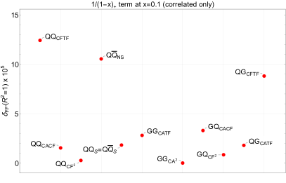
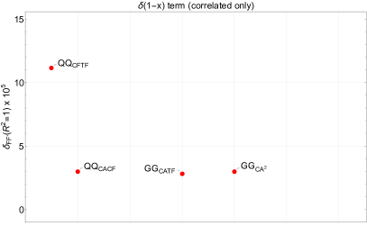
Figure 1: The quantity $\delta_{FF^{\prime}}(R^{2})$ as defined in Eq. (53) evaluated at $R=1$ for the different flavour channels for the $1/(1-x)_{+}$ contribution at $x=0.1$ (left) and the $\delta(1-x)$ contribution (right). Note that, as indicated on the $y$ axis, each value of $\delta_{FF^{\prime}}(R^{2})$ has been multiplied by a factor of $10^{5}$.

4 Numerical computation of the quark and gluon beam functions

We now discuss a numerical evaluation of the quark and gluon beam functions, which provides a crucial consistency check of the analytic results discussed in the previous section. In this section, we first outline the steps followed in the numerical calculation and then present a comparison between our numerical and analytic results.

4.1 Method for the numerical computation

All numerical integrations discussed below are performed using the GlobalAdaptive NIntegrate routine from Mathematica, to an accuracy at the permyriad level or better. This will allow for precise numerical tests of the analytic calculation.

The correlated correction.

For this part of the beam function, the integrand can only have a rapidity divergence as $\eta_{t}\equiv\tfrac{1}{2}(\eta_{1}+\eta_{2})\to-\infty$ at finite $\eta\equiv\eta_{1}-\eta_{2}$, corresponding to $x\to 1$. Note that the restriction $k_{1}^{-}+k_{2}^{-}<p^{-}$ forbids us from approaching $\eta_{t}\to\infty$ and encountering a rapidity divergence in this limit. We find it convenient to choose integration variables that remain finite as $\eta_{t}\to-\infty$ (at finite $k_{1\perp}^{2}$, $k_{2\perp}^{2}$, $\eta$). In this way, $x$ controls the approach to the rapidity divergence. Explicitly, we choose

$$\mathcal{Z}\equiv\dfrac{k_{1}^{+}}{k_{1}^{+}+k_{2}^{+}}\,,\quad\mathcal{T}\equiv(k_{1}^{+}+k_{2}^{+})(k_{1}^{-}+k_{2}^{-})\,,$$ (54)

along with $\eta$ and the azimuthal separation between the two emitted partons, $\phi$.

Using these variables, the rapidity divergences manifest themselves as a factor of $1/(1-x)$ in the squared amplitude. This is regulated by inserting the exponential regulator factor (20), where in the exponent we may drop the $k^{-}\equiv k_{1}^{-}+k_{2}^{-}$ as we do not encounter any rapidity divergences associated with $k_{1}^{-},k_{2}^{-}\to\infty$. We take the limit $\nu\to+\infty$ in the regulator and make use of the distributional expansion given in Eq. (3.5) of Luo:2019hmp :

$$\frac{e^{-\frac{1}{\nu\,(1-x)}}}{1-x}=(\ln\nu-\gamma_{E})\,\delta(1-x)+\frac{1}{(1-x)_{+}}+\mathcal{O}(\nu^{-1})\,.$$ (55)

The structure of the integrand in $\mathcal{T}$ is simple, containing only terms of the form $\log^{n}(\mathcal{T})/\mathcal{T}$, and integration over this variable may be done analytically. This just leaves the integrations over $\mathcal{Z}$, $\eta$, and $\phi$, which are performed numerically at fixed values of $x$ and $R$.

The uncorrelated correction.

After symmetrisation of the integrand in partons $k_{1}$ and $k_{2}$, we may choose to integrate only over $\eta<0$ and then multiply the final result by $2$. With this restriction, for the uncorrelated contribution to the squared amplitude we encounter rapidity divergences as $\eta_{1}\to-\infty$, as well as when $\eta_{t}\to-\infty$. For our integration variables we should choose two variables that control the approaches to these two limits, and then other variables that remain finite in these limits. We choose to use:

$$\chi_{1}\equiv k_{2}^{+}(k_{1}^{-}+k_{2}^{-}),\quad\chi_{2}\equiv\dfrac{k_{1}^{-}(k_{1}^{+}+k_{2}^{+})^{2}}{k_{1}^{+}k^{2}_{2\perp}},\quad\overline{\mathcal{Z}}=1-\mathcal{Z}\,,$$ (56)

as well as $x$ and $\phi$. Then, the limit $\eta_{1}\to-\infty$ corresponds to $\overline{\mathcal{Z}}\to 0$, whilst $\eta_{t}\to-\infty$ corresponds to $x\to 1$ and the rapidity divergences manifest themselves as a factor $1/[\overline{\mathcal{Z}}(1-x)]$ in the integrand. We insert the exponential regulator (again, we can drop the $k^{+}$ in the exponent), and make use of the distributional expansion given in Eq. (3.30) of Ref. Luo:2019hmp :

$$\frac{1}{(1-x)\overline{\mathcal{Z}}}\exp\left(-\frac{1}{\nu(1-x)\overline{\mathcal{Z}}}\right)=\left(\frac{1}{2}(\ln\nu-\gamma_{E})^{2}+\frac{\pi^{2}}{12}\right)\delta(1-x)\,\delta(\overline{\mathcal{Z}})+\frac{1}{(1-x)_{+}}\frac{1}{\overline{\mathcal{Z}}_{+}}$$

$$+\left(\bigg{[}\frac{\ln\overline{\mathcal{Z}}}{\overline{\mathcal{Z}}}\bigg{]}_{+}+\frac{\ln\nu-\gamma_{E}}{\overline{\mathcal{Z}}_{+}}\right)\delta(1-x)+\left(\bigg{[}\frac{\ln(1-x)}{1-x}\bigg{]}_{+}+\frac{\ln\nu-\gamma_{E}}{(1-x)_{+}}\right)\delta(\overline{\mathcal{Z}})+\mathcal{O}(\nu^{-1})\,.$$ (57)

We perform the integration over $\chi_{1}$ analytically, and the integrations over the $\chi_{2}$, $\overline{\mathcal{Z}}$ and $\phi$ variables numerically (for terms containing a $\delta(\overline{\mathcal{Z}})$, we perform the trivial $\overline{\mathcal{Z}}$ integration analytically).

The soft-collinear zero bins.

We use the approach of Refs. Tackmann:2012bt ; Stewart:2013faa as a way to compute the zero-bin subtraction without performing the multipole expansion of the measurement function, see Sec. 3.3 and in particular Eq. (51). Let us, without loss of generality, take parton $k_{1}$ to be soft. Then $k_{1}^{-}$ is no longer restricted by the delta function on the minus light-cone momentum, and we may have rapidity divergences for $\eta_{1}\to\pm\infty$ as well as for $\eta_{2}\to-\infty$. We handle this calculation by re-expressing the clustering constraint in the measurement as:

$$\Theta(\eta^{2}+\phi^{2}-R^{2})=1-\Theta(R^{2}-\eta^{2}-\phi^{2})\,.$$ (58)

In the second term on the right hand side, the two partons are restricted to be close together in rapidity, such that we only have rapidity divergences corresponding to $\eta_{t}\to-\infty$ (or $x\to 1$). The same strategy may then be used for this term as was used for the correlated corrections. Note that there is no collinear divergence here associated with $\eta,\phi\to 0$, due to the form of the squared amplitude for the soft-collinear zero bin (which coincides with the squared amplitude for the uncorrelated correction).

For the first term on the right-hand side of Eq. (58), we choose to use the same variables we used in Ref. Abreu:2022sdc :

$$\mathcal{K}^{2}_{T}=k_{1\perp}^{2}+k_{2\perp}^{2}\,,\qquad z=\dfrac{k_{1\perp}^{2}}{k_{1\perp}^{2}+k_{2\perp}^{2}}\,,$$ (59)

along with $\eta_{1}$, $\phi$ and $x$. The approach to $\eta_{2}\to-\infty$ is then controlled by $x$, whilst $\eta_{1}$ directly controls the approach to $\eta_{1}\to\pm\infty$. We introduce the exponential regulator, and split it in a straightforward way into two factors depending on $k_{1}$ and $k_{2}$ respectively; we drop the $k_{2}^{+}$ in the exponent as before, but now may no longer drop $k_{1}^{+}$. The integrand does not depend on $\eta_{1}$ (except in the regulator factor), and we may perform the integral over $\eta_{1}$ using Eq. (3.24) from Ref. Abreu:2022sdc . We utilise Eq. (4.1) for the rapidity divergence corresponding to $x\to 1$. The integration over $\mathcal{K}^{2}_{T}$ is performed analytically, and the $z$ and $\phi$ integrals are done numerically.

The soft-soft zero bins.

This calculation coincides exactly with that performed in Ref. Abreu:2022sdc (up to a prefactor of $\delta(1-x)$ that appears here), and we use the results presented in that paper for this contribution.

4.2 Comparison with the analytic results

As a further assessment of the quality of our analytic small-$R$ expansion, we compare the numerical calculations (which have exact $R$ dependence) with the analytic results obtained in the previous section at different values of $R$. Due to the many flavour channels, we choose to show here only the worst-case scenario, namely the comparison between the two calculations for the most complicated contributions, corresponding to the correlated part of the squared amplitudes in Eq. (35). Fig. 2 shows the outcome of this comparison at $R=1$, and we can see that the difference between the two computations is at the level of parts per million, which is the level of accuracy of the numerical calculation. This demonstrates that the $R$ expansion converges extremely well up to $R=1$.

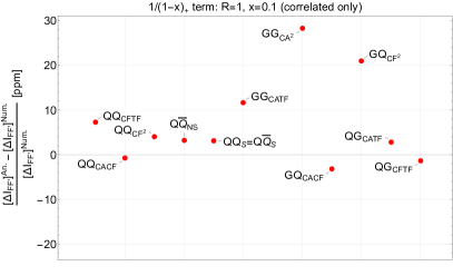
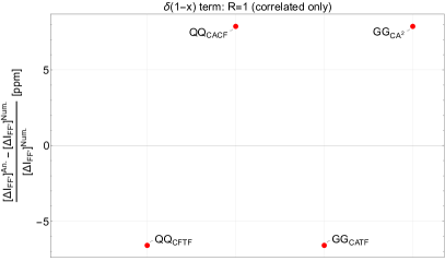
Figure 2: Difference, in parts per million, between the analytic result and the numerical calculation with full $R$ dependence for the correlated contribution to the unsubtracted beam functions. The figures show the coefficient of $1/(1-x)_{+}$ at $x=0.1$ (left plot) and the coefficient of $\delta(1-x)$ (right plot), both evaluated at $R=1$. The different labels denote the various colour structures contributing to each flavour channel. The size of the difference is always at the level of the precision of the numerical calculation.

5 Leading-jet $p_{T}$ slicing at NNLO

The computation of the two-loop beam functions for the leading-jet $p_{T}$ constitutes the last missing ingredient to construct a non-local subtraction scheme for colour singlet production at NNLO based on $p_{T}^{\rm jet}$. In analogy with non-local subtraction schemes such as $q_{T}$-subtraction Catani:2007vq , jettiness subtraction Boughezal:2015dva ; Gaunt:2015pea , and $k_{T}^{\rm ness}$ subtraction Buonocore:2022mle , we can formulate an NNLO slicing fully differential in the Born phase space for the production of a colour singlet $F$, as (${d}\sigma\equiv\frac{{d}\sigma}{{d}\Phi_{\rm Born}}$)

$${d}\sigma^{F}_{\rm NNLO} =\mathbb{H}^{\rm NNLO}_{\rm veto}\otimes{d}\sigma_{\rm Born}+\lim_{p_{T,\rm cut}^{\rm jet}\rightarrow 0}\int_{p_{T,\rm cut}^{\rm jet}}^{+\infty}{d}p_{T}^{\rm jet}\left(\frac{{d}^{2}\sigma^{F+\rm jet}_{\rm NLO}}{{d}p_{T}^{\rm jet}}-\frac{{d}^{2}\sigma(p_{T}^{\rm veto})}{{d}p_{T}^{\rm veto}}\Bigg{|}_{p_{T}^{\rm veto}=p_{T}^{\rm jet}}^{(\alpha_{s}^{2})}\right),$$ (60)

where the first term on the right hand side coincides with the non-logarithmic terms of the jet-veto cross section Eq. (2), the last term is its derivative with respect to $p_{T}^{\rm veto}$ expanded through ${\cal O}(\alpha_{s}^{2})$ relative to the Born, and the second term is the NLO cross-section for the production of the colour singlet in association with a jet. The above formula formally reduces to the NNLO result in the limit $p_{T,\rm cut}^{\rm jet}~{}\rightarrow~{}0$. However, since the second and the third terms are both divergent logarithmically in this limit, Eq. (60) can be computed numerically only by choosing a finite value of $p_{T,\rm cut}^{\rm jet}~{}>~{}0$. This introduces a slicing error $\mathcal{O}((p_{T,\rm cut}^{\rm jet}/Q)^{m})$, where $m$ is an integer value to be determined by studying the $p_{T,\rm cut}^{\rm jet}\rightarrow 0$ behaviour of the non-singular contribution contained within brackets in Eq. (60).

The comparison of the NNLO results obtained using Eq. (60) to the known NNLO cross sections provides a very robust check of the correctness of the results presented in this work. We perform this test by considering on-shell $Z$ and $H$ production, which allows us to independently check the quark and gluon beam functions, respectively. We use MCFM 9.1 Campbell:2019dru to compute the NLO result for $Z+j$ Giele:1993dj and $H+j$ deFlorian:1999zd ; Ravindran:2002dc ; Glosser:2002gm production, while we use the implementation of the jet-veto resummation Becher:2012qa ; Banfi:2012jm ; Stewart:2013faa ; Becher:2013xia in the RadISH code Monni:2016ktx ; Bizon:2017rah ; Monni:2019yyr to compute the factorised expression (2) and its expansion up to NNLO. We compare our results with the analytic NNLO cross section for $Z$ Hamberg:1990np ; vanNeerven:1991gh and $H$ Ravindran:2002dc ; Ravindran:2003um ; Harlander:2002wh production which we computed using the n3loxs code. For our numerical checks, we consider proton-proton collisions at a centre-of-mass energy of 13 TeV and $R=0.4$. We adopt the LUXqed_plus_PDF4LHC15_nnlo_100 parton distribution functions Manohar:2017eqh through the LHAPDF interface Buckley:2014ana . We choose factorisation and resummation scales equal to $\mu_{R}=\mu_{F}=m_{Z},m_{H}$ for $Z$ and $H$ production, respectively, with $m_{Z}=91.1876$ and $m_{H}=125$ GeV. In Fig. 3 we study the dependence of the NNLO correction on $p_{T,\rm cut}^{\rm jet}/Q$ for $Z$ and $H$ production for different partonic channels by normalising it to the analytic result. We compare the results obtained using $p_{T}^{\rm jet}$-slicing (in orange) with those obtained using $q_{T}$-slicing (in blue) to assess the performance of the two methods. For $Z$ production we are able to lower the value of $p_{T,\rm cut}^{\rm jet}$ down to $0.1$ GeV, whereas we stop at $p_{T,\rm cut}^{\rm jet}=0.5$ GeV for Higgs production as the fixed order $H+j$ calculation becomes slightly unstable in some channels below this value. We observe that in all the channels the results obtained using leading-jet $p_{T}$ slicing converge to the exact cross section in the $p_{T,\rm cut}^{\rm jet}\rightarrow 0$ limit, thus providing a powerful check of the validity of our computations. By comparing the results obtained with $p_{T}^{\rm jet}$-slicing to those obtained using $q_{T}$-slicing we notice that the convergence towards the analytic result is comparable between the two methods, with $q_{T}$-slicing converging slightly faster in most cases for $R=0.4$. Smaller values of the jet radius $R$ appear to improve the convergence of the $p_{T}^{\rm jet}$ subtraction, possibly due to the reduced size of the subleading power corrections. Further investigations on the size of subleading power corrections deserve dedicated studies.

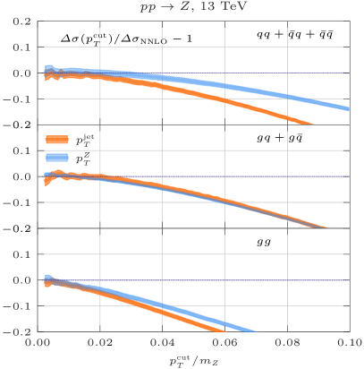
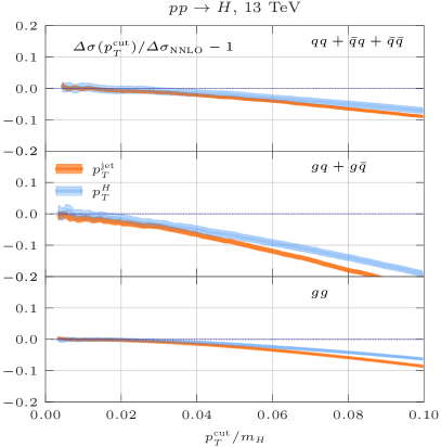
Figure 3: NNLO correction for $Z$ (left panel) and $H$ (right panel) production: leading-jet $p_{T}$ subtraction (blue) against $q_{T}$ subtraction (blue) and analytic results.

6 Conclusions

In this article, we presented the first calculation of the complete set of two-loop beam functions relevant for the leading-jet transverse momentum resummation in colour singlet production. The results were obtained using two independent methods: a semi-analytical expansion for small jet-radius $R$ up to and including terms of $\mathcal{O}(R^{8})$, and a fully numerical evaluation for several fixed values of $R$. The small-$R$ expansion is analytical with the only exception being a set of $R$-independent regular terms. The numerical calculation retains the complete $R$ dependence and shows perfect agreement with the analytical expansion in the range $R\in[0,1]$ which is relevant for collider phenomenology. We further checked our computation by performing an NNLO calculation of the total cross section for Higgs and $Z$ boson production using a slicing subtraction scheme based on the leading-jet $p_{T}$. Our calculation reproduces known analytic predictions for the NNLO total cross section in all flavour channels, thus validating our results.

When describing the technical aspects of the calculation, we discussed in detail the complications related to zero-bin subtraction and soft-collinear mixing. In particular, we explicitly showed that if one performs a multipole expansion of the measurement functions there exist no mixed soft-collinear contributions which break the SCET factorisation theorem at NNLO. This observation is non-trivial in the presence of the exponential rapidity regulator in that it adds a new scale to the problem, which leads to the presence of non-vanishing integrals that would otherwise be scaleless.

Our complete results are provided in Mathematica-readable files attached to the arXiv version of this article. Together with our earlier analytic results for the leading-jet $p_{T}$ soft function Abreu:2022sdc , they constitute an important step towards the N³LL resummation of this observable, with the only missing ingredient being the three-loop rapidity anomalous dimension.

Note added

In the final stages of the preparation of this article, Ref. Bell:2022nrj appeared with a numerical calculation of the beam functions in the quark channel. These results are obtained with a different rapidity regulator and computed for a discrete set of real points in the Mellin variable $N$ conjugate to the longitudinal momentum $x$. For this reason, it is not immediately clear how to compare the results of Ref. Bell:2022nrj with the ones presented here.

Appendix A Expansion of the exponential regulator in zero-bin integrals

In this appendix we provide the ingredients to calculate the integrals contributing to the zero-bin subtraction discussed in Sec. 3.3. Specifically, we provide the analogues of Eqs. (3.2), (40) needed for the calculation of the correlated and uncorrelated contributions, respectively.

Soft-collinear zero-bin.

We consider the limit in which one of the two partons is soft (say $k_{2}$) and the second is collinear. The exponential regulator in the correlated corrections can be expanded as:

$$\int{d}\eta_{1} \,e^{-2k_{1\perp}\frac{e^{-\gamma_{E}}}{\nu}[\cosh{(\eta_{1})}+\zeta\cosh{(\eta-\eta_{1})}]}\,\delta(k_{1}^{-}-(1-x)p^{-})$$

$$= \frac{1}{p^{-}}\left[\left(-\ln\left(1+e^{-\eta}\zeta\right)+\ln\frac{p^{-}\nu}{k_{1\perp}^{2}}\right)\delta(1-x)+\frac{1}{(1-x)_{+}}+{\cal O}(\nu^{-1})\right]\,.$$ (61)

Similarly, we can use the following formula to deal with the uncorrelated contribution (see footnote 3):

$$\int{d}\eta_{1} {d}\eta\,e^{-2k_{1\perp}\frac{e^{-\gamma_{E}}}{\nu}[\cosh{(\eta_{1})}+\zeta\cosh{(\eta-\eta_{1})}]}\,\delta(k_{1}^{-}-(1-x)p^{-})$$ (62)

$$= \frac{1}{p^{-}}\int{d}w\left[\frac{1}{(w)_{+}}\frac{1}{(1-x)_{+}}-\frac{2}{(1-x)_{+}}\left(\ln(\zeta)-\ln\left(\frac{\nu}{k_{1\perp}}\right)\right)\delta(w)\right.$$

$$\left.\left[-\left(\frac{\ln\left(1+w^{-1}\zeta\right)}{w}\right)_{+}+\ln\left(\frac{p^{-}\nu}{k^{2}_{1\perp}}\right)\frac{1}{(w)_{+}}\right]\,\delta(1-x)\right.$$

$$\left.-2\left(\ln(\zeta)-\ln\left(\frac{\nu}{k_{1\perp}}\right)\right)\ln\left(\frac{p^{-}\nu}{k^{2}_{1\perp}}\right)\delta(w)\,\delta(1-x)+{\cal O}(\nu^{-1})\right]\,.$$

Analogous expressions hold for the case in which $k_{1}$ is soft.

Double-soft zero-bin.

In the limit in which both partons are soft, the exponential regulator in the correlated corrections can be expanded as:

$$\int{d}\eta_{1} \,e^{-2k_{1\perp}\frac{e^{-\gamma_{E}}}{\nu}[\cosh{(\eta_{1})}+\zeta\cosh{(\eta-\eta_{1})}]}\,\delta((1-x)p^{-})$$

$$= \frac{1}{p^{-}}\left[\left(-\ln\left((e^{\eta}+\zeta)(e^{-\eta}+\zeta)\right)+\ln\frac{\nu^{2}}{k_{1\perp}^{2}}\right)\delta(1-x)+{\cal O}(\nu^{-1})\right]\,,$$ (63)

and in the uncorrelated correction as (see footnote 3):

$$\int{d}\eta_{1} {d}\eta\,e^{-2k_{1\perp}\frac{e^{-\gamma_{E}}}{\nu}[\cosh{(\eta_{1})}+\zeta\cosh{(\eta-\eta_{1})}]}\,\delta((1-x)p^{-})$$ (64)

$$= \frac{1}{p^{-}}\int{d}w\left[-\left[\left(\frac{\ln\left(\left(w^{-1}+\zeta\right)\left(w+\zeta\right)\right)}{w}\right)_{+}-2\ln\left(\frac{\nu}{k_{1\perp}}\right)\frac{1}{(w)_{+}}\right]\,\delta(1-x)\right.$$

$$\left.-4\ln\left(\frac{\nu}{k_{1\perp}}\right)\left(\ln(\zeta)-\ln\left(\frac{\nu}{k_{1\perp}}\right)\right)\delta(w)\,\delta(1-x)+{\cal O}(\nu^{-1})\right]\,.$$

References

- (1) A. Banfi, G. P. Salam and G. Zanderighi, NLL+NNLO predictions for jet-veto efficiencies in Higgs-boson and Drell-Yan production, JHEP 06 (2012) 159, [1203.5773].
- (2) T. Becher and M. Neubert, Factorization and NNLL Resummation for Higgs Production with a Jet Veto, JHEP 07 (2012) 108, [1205.3806].
- (3) A. Banfi, P. F. Monni, G. P. Salam and G. Zanderighi, Higgs and Z-boson production with a jet veto, Phys. Rev. Lett. 109 (2012) 202001, [1206.4998].
- (4) A. Banfi, P. F. Monni and G. Zanderighi, Quark masses in Higgs production with a jet veto, JHEP 01 (2014) 097, [1308.4634].
- (5) T. Becher, M. Neubert and L. Rothen, Factorization and +NNLO predictions for the Higgs cross section with a jet veto, JHEP 10 (2013) 125, [1307.0025].
- (6) I. W. Stewart, F. J. Tackmann, J. R. Walsh and S. Zuberi, Jet resummation in Higgs production at , Phys. Rev. D 89 (2014) 054001, [1307.1808].
- (7) A. Banfi, F. Caola, F. A. Dreyer, P. F. Monni, G. P. Salam, G. Zanderighi et al., Jet-vetoed Higgs cross section in gluon fusion at N3LO+NNLL with small- resummation, JHEP 04 (2016) 049, [1511.02886].
- (8) T. Becher, R. Frederix, M. Neubert and L. Rothen, Automated NNLL NLO resummation for jet-veto cross sections, Eur. Phys. J. C 75 (2015) 154, [1412.8408].
- (9) I. Moult and I. W. Stewart, Jet Vetoes interfering with , JHEP 09 (2014) 129, [1405.5534].
- (10) P. Jaiswal and T. Okui, Explanation of the excess at the LHC by jet-veto resummation, Phys. Rev. D 90 (2014) 073009, [1407.4537].
- (11) P. F. Monni and G. Zanderighi, On the excess in the inclusive cross section, JHEP 05 (2015) 013, [1410.4745].
- (12) Y. Wang, C. S. Li and Z. L. Liu, Resummation prediction on gauge boson pair production with a jet veto, Phys. Rev. D 93 (2016) 094020, [1504.00509].
- (13) S. Dawson, P. Jaiswal, Y. Li, H. Ramani and M. Zeng, Resummation of jet veto logarithms at N3LLa + NNLO for production at the LHC, Phys. Rev. D 94 (2016) 114014, [1606.01034].
- (14) P. F. Monni, L. Rottoli and P. Torrielli, Higgs transverse momentum with a jet veto: a double-differential resummation, Phys. Rev. Lett. 124 (2020) 252001, [1909.04704].
- (15) S. Kallweit, E. Re, L. Rottoli and M. Wiesemann, Accurate single- and double-differential resummation of colour-singlet processes with MATRIX+RADISH: production at the LHC, JHEP 12 (2020) 147, [2004.07720].
- (16) S. Abreu, J. R. Gaunt, P. F. Monni and R. Szafron, The analytic two-loop soft function for leading-jet , 2204.02987.
- (17) C. W. Bauer, S. Fleming, D. Pirjol and I. W. Stewart, An Effective field theory for collinear and soft gluons: Heavy to light decays, Phys. Rev. D 63 (2001) 114020, [hep-ph/0011336].
- (18) C. W. Bauer, D. Pirjol and I. W. Stewart, Soft collinear factorization in effective field theory, Phys. Rev. D 65 (2002) 054022, [hep-ph/0109045].
- (19) C. W. Bauer, S. Fleming, D. Pirjol, I. Z. Rothstein and I. W. Stewart, Hard scattering factorization from effective field theory, Phys. Rev. D 66 (2002) 014017, [hep-ph/0202088].
- (20) M. Beneke, A. P. Chapovsky, M. Diehl and T. Feldmann, Soft collinear effective theory and heavy to light currents beyond leading power, Nucl. Phys. B 643 (2002) 431–476, [hep-ph/0206152].
- (21) M. Beneke and T. Feldmann, Multipole expanded soft collinear effective theory with nonAbelian gauge symmetry, Phys. Lett. B 553 (2003) 267–276, [hep-ph/0211358].
- (22) M. Beneke, Helmholtz International Summer School on Heavy Quark Physics, Dubna, 2005.
- (23) T. Becher and M. Neubert, Drell-Yan Production at Small , Transverse Parton Distributions and the Collinear Anomaly, Eur. Phys. J. C 71 (2011) 1665, [1007.4005].
- (24) Y. Li, D. Neill and H. X. Zhu, An exponential regulator for rapidity divergences, Nucl. Phys. B 960 (2020) 115193, [1604.00392].
- (25) F. J. Tackmann, J. R. Walsh and S. Zuberi, Resummation Properties of Jet Vetoes at the LHC, Phys. Rev. D 86 (2012) 053011, [1206.4312].
- (26) J.-y. Chiu, A. Jain, D. Neill and I. Z. Rothstein, The Rapidity Renormalization Group, Phys. Rev. Lett. 108 (2012) 151601, [1104.0881].
- (27) J.-Y. Chiu, A. Jain, D. Neill and I. Z. Rothstein, A Formalism for the Systematic Treatment of Rapidity Logarithms in Quantum Field Theory, JHEP 05 (2012) 084, [1202.0814].
- (28) T. Becher and M. Neubert, Threshold resummation in momentum space from effective field theory, Phys. Rev. Lett. 97 (2006) 082001, [hep-ph/0605050].
- (29) T. Matsuura and W. L. van Neerven, Second Order Logarithmic Corrections to the Drell-Yan Cross-section, Z. Phys. C 38 (1988) 623.
- (30) T. Gehrmann, T. Huber and D. Maitre, Two-loop quark and gluon form-factors in dimensional regularisation, Phys. Lett. B 622 (2005) 295–302, [hep-ph/0507061].
- (31) S. Moch, J. A. M. Vermaseren and A. Vogt, The Three loop splitting functions in QCD: The Nonsinglet case, Nucl. Phys. B 688 (2004) 101–134, [hep-ph/0403192].
- (32) T. Gehrmann, E. W. N. Glover, T. Huber, N. Ikizlerli and C. Studerus, Calculation of the quark and gluon form factors to three loops in QCD, JHEP 06 (2010) 094, [1004.3653].
- (33) Y. Li, A. von Manteuffel, R. M. Schabinger and H. X. Zhu, Soft-virtual corrections to Higgs production at N3LO, Phys. Rev. D 91 (2015) 036008, [1412.2771].
- (34) M. Cacciari, G. P. Salam and G. Soyez, FastJet User Manual, Eur. Phys. J. C 72 (2012) 1896, [1111.6097].
- (35) M. Cacciari, G. P. Salam and G. Soyez, The anti- jet clustering algorithm, JHEP 04 (2008) 063, [0802.1189].
- (36) Y. L. Dokshitzer, G. D. Leder, S. Moretti and B. R. Webber, Better jet clustering algorithms, JHEP 08 (1997) 001, [hep-ph/9707323].
- (37) M. Wobisch and T. Wengler, Hadronization corrections to jet cross-sections in deep inelastic scattering, in Workshop on Monte Carlo Generators for HERA Physics (Plenary Starting Meeting), pp. 270–279, 4, 1998. hep-ph/9907280.
- (38) S. Catani, Y. L. Dokshitzer, M. H. Seymour and B. R. Webber, Longitudinally invariant clustering algorithms for hadron hadron collisions, Nucl. Phys. B 406 (1993) 187–224.
- (39) T. Gehrmann, T. Luebbert and L. L. Yang, Calculation of the transverse parton distribution functions at next-to-next-to-leading order, JHEP 06 (2014) 155, [1403.6451].
- (40) M. G. Echevarria, I. Scimemi and A. Vladimirov, Unpolarized Transverse Momentum Dependent Parton Distribution and Fragmentation Functions at next-to-next-to-leading order, JHEP 09 (2016) 004, [1604.07869].
- (41) M.-X. Luo, X. Wang, X. Xu, L. L. Yang, T.-Z. Yang and H. X. Zhu, Transverse Parton Distribution and Fragmentation Functions at NNLO: the Quark Case, JHEP 10 (2019) 083, [1908.03831].
- (42) M.-X. Luo, T.-Z. Yang, H. X. Zhu and Y. J. Zhu, Transverse Parton Distribution and Fragmentation Functions at NNLO: the Gluon Case, JHEP 01 (2020) 040, [1909.13820].
- (43) M.-x. Luo, T.-Z. Yang, H. X. Zhu and Y. J. Zhu, Quark Transverse Parton Distribution at the Next-to-Next-to-Next-to-Leading Order, Phys. Rev. Lett. 124 (2020) 092001, [1912.05778].
- (44) M. A. Ebert, B. Mistlberger and G. Vita, Transverse momentum dependent PDFs at N3LO, JHEP 09 (2020) 146, [2006.05329].
- (45) S. Catani and M. Grazzini, QCD transverse-momentum resummation in gluon fusion processes, Nucl. Phys. B 845 (2011) 297–323, [1011.3918].
- (46) D. Gutierrez-Reyes, S. Leal-Gomez, I. Scimemi and A. Vladimirov, Linearly polarized gluons at next-to-next-to leading order and the Higgs transverse momentum distribution, JHEP 11 (2019) 121, [1907.03780].
- (47) J. Gaunt, M. Stahlhofen and F. J. Tackmann, The Gluon Beam Function at Two Loops, JHEP 08 (2014) 020, [1405.1044].
- (48) J. R. Gaunt, M. Stahlhofen and F. J. Tackmann, The Quark Beam Function at Two Loops, JHEP 04 (2014) 113, [1401.5478].
- (49) S. Gangal, J. R. Gaunt, M. Stahlhofen and F. J. Tackmann, Two-Loop Beam and Soft Functions for Rapidity-Dependent Jet Vetoes, JHEP 02 (2017) 026, [1608.01999].
- (50) A. Banfi, H. McAslan, P. F. Monni and G. Zanderighi, A general method for the resummation of event-shape distributions in annihilation, JHEP 05 (2015) 102, [1412.2126].
- (51) C. Duhr and F. Dulat, PolyLogTools — polylogs for the masses, JHEP 08 (2019) 135, [1904.07279].
- (52) M. Beneke and V. A. Smirnov, Asymptotic expansion of Feynman integrals near threshold, Nucl. Phys. B 522 (1998) 321–344, [hep-ph/9711391].
- (53) A. V. Manohar and I. W. Stewart, The Zero-Bin and Mode Factorization in Quantum Field Theory, Phys. Rev. D 76 (2007) 074002, [hep-ph/0605001].
- (54) S. Catani and M. Grazzini, An NNLO subtraction formalism in hadron collisions and its application to Higgs boson production at the LHC, Phys. Rev. Lett. 98 (2007) 222002, [hep-ph/0703012].
- (55) R. Boughezal, C. Focke, X. Liu and F. Petriello, -boson production in association with a jet at next-to-next-to-leading order in perturbative QCD, Phys. Rev. Lett. 115 (2015) 062002, [1504.02131].
- (56) J. Gaunt, M. Stahlhofen, F. J. Tackmann and J. R. Walsh, N-jettiness Subtractions for NNLO QCD Calculations, JHEP 09 (2015) 058, [1505.04794].
- (57) L. Buonocore, M. Grazzini, J. Haag, L. Rottoli and C. Savoini, Effective transverse momentum in multiple jet production at hadron colliders, 2201.11519.
- (58) J. Campbell and T. Neumann, Precision Phenomenology with MCFM, JHEP 12 (2019) 034, [1909.09117].
- (59) W. T. Giele, E. W. N. Glover and D. A. Kosower, Higher order corrections to jet cross-sections in hadron colliders, Nucl. Phys. B 403 (1993) 633–670, [hep-ph/9302225].
- (60) D. de Florian, M. Grazzini and Z. Kunszt, Higgs production with large transverse momentum in hadronic collisions at next-to-leading order, Phys. Rev. Lett. 82 (1999) 5209–5212, [hep-ph/9902483].
- (61) V. Ravindran, J. Smith and W. L. Van Neerven, Next-to-leading order QCD corrections to differential distributions of Higgs boson production in hadron hadron collisions, Nucl. Phys. B 634 (2002) 247–290, [hep-ph/0201114].
- (62) C. J. Glosser and C. R. Schmidt, Next-to-leading corrections to the Higgs boson transverse momentum spectrum in gluon fusion, JHEP 12 (2002) 016, [hep-ph/0209248].
- (63) P. F. Monni, E. Re and P. Torrielli, Higgs Transverse-Momentum Resummation in Direct Space, Phys. Rev. Lett. 116 (2016) 242001, [1604.02191].
- (64) W. Bizon, P. F. Monni, E. Re, L. Rottoli and P. Torrielli, Momentum-space resummation for transverse observables and the Higgs p⟂ at N3LL+NNLO, JHEP 02 (2018) 108, [1705.09127].
- (65) R. Hamberg, W. L. van Neerven and T. Matsuura, A complete calculation of the order correction to the Drell-Yan factor, Nucl. Phys. B 359 (1991) 343–405.
- (66) W. L. van Neerven and E. B. Zijlstra, The corrected Drell-Yan factor in the DIS and MS scheme, Nucl. Phys. B 382 (1992) 11–62.
- (67) V. Ravindran, J. Smith and W. L. van Neerven, NNLO corrections to the total cross-section for Higgs boson production in hadron hadron collisions, Nucl. Phys. B 665 (2003) 325–366, [hep-ph/0302135].
- (68) R. V. Harlander and W. B. Kilgore, Next-to-next-to-leading order Higgs production at hadron colliders, Phys. Rev. Lett. 88 (2002) 201801, [hep-ph/0201206].
- (69) A. V. Manohar, P. Nason, G. P. Salam and G. Zanderighi, The Photon Content of the Proton, JHEP 12 (2017) 046, [1708.01256].
- (70) A. Buckley, J. Ferrando, S. Lloyd, K. Nordström, B. Page, M. Rüfenacht et al., LHAPDF6: parton density access in the LHC precision era, Eur. Phys. J. C 75 (2015) 132, [1412.7420].
- (71) X. Chen, J. Cruz-Martinez, T. Gehrmann, E. W. N. Glover and M. Jaquier, NNLO QCD corrections to Higgs boson production at large transverse momentum, JHEP 10 (2016) 066, [1607.08817].
- (72) G. Bell, K. Brune, G. Das and M. Wald, The NNLO quark beam function for jet-veto resummation, 2207.05578.