Experimental emulation for OTFS waveform RF-impairments

Abstract

Orthogonal time-frequency space (OTFS) waveform exceeds the challenges that face orthogonal frequency division multiplexing (OFDM) in the high-mobility environment with high time-frequency dispersive channels. Since practical pulse shaping design and RF-impairments effects have a direct impact on waveform behavior, this paper investigates experimental implementation for practical pulse shaping design and RF-impairments that affect OTFS waveform performance and compares them to OFDM waveform as a benchmark. Firstly, the doubly-dispersive channel effect is analyzed, then an experimental framework is established for investigating the RF-impairments include non-linearity, Carrier frequency offset, I/Q-imbalances, DC-offset, and phase noise are considered. The experiments were conducted in a real indoor wireless environment using software-defined radio (SDR)based on the Keysight EXG X-Serie devices. The experimental results validate the accuracy of the theoretical results.

I Introduction

TABLE I: NOMENCLATURES

Abbreviation	Definition
5G	Fifth Generation
6G	Sixth Generation
A/D	Analogto-Digital
BER	Bit Error Rate
CCDF	Cumulative Distribution Function
CFO	Carrier Frequency Offset
CP	Cyclic Prefix
D/A	Digital-To-Analog()
DC	Direct Current
eMBB	Enhanced-Mobile Broadband
I/Q imbalance	In-Phase And Quadrature Imbalance
ICF	Iterative Clipping And Filtering
ICI	Iter-Carrier Interference
ISFFT	inverse symplectic finite Fourier transform
ISI	Inter-Symbol Interference
JRC	Joint Radar Communication
LNA	Low-Noise Amplifier
LS	Least Squares
MIMO	Multi-Input Multi Output
mMTC	Massive Machine Type Communications
mmWave	millimeter wave
MP	Message Passing
NOMA	Non-Orthogonal Multiple Access
OFDM	Orthogonal Frequency Division Multiplexing
OTFS	Orthogonal Time-Frequency Space
PA	Power Amplifier
PAPR	Peak-To-Average Power Ratio
PSW	Prolate Spheroida Waveform
QAM	Quadrature Amplitude Modulation
RF	Radio-Frequency
SDR	Software-Defined Radio
SFFT	Symplectic Finite Fourier Transform
URLLC	Ultra-Reliable And Low Latency Communications
VSA	Vector Signal Analyzer
VSG	Vector Signal Generator
RCF	Raised-cosine filter
LO	Local oscillator
HPA	high power amplifier
OOB	out-of-band
AWGN	additive white Gaussian noise
CMOS	complementary metal-oxide-semiconductor
VCO	voltage control oscillator

The exponential growth in the number of connected devices created an urge to differentiate and fulfill the various requirements of the users in the network so that all are served properly[1]. These needs are the main driving factors of the 5G, that mainly support three services i.e., enhanced-mobile broadband (eMBB), ultra-reliable and low latency communications (URLLC), and massive machine type communications (mMTC). These different services are achieved by using multiple OFDM numerologies [2, 3]. The same concept is visioned for the 6G, where instead of implementing OFDM with multiple parameters, the network will be ultra-flexible and will accommodate multiple different waveforms in a single frame to meet the requirements of the 6G [4].

One of the most promising waveform candidates is the OTFS waveform, that represents the information symbols in the delay-Doppler domain, where all modulated data experiences almost the same channel gain even at high mobility cases [5]. This enhances the performance of the system that suffers from high Doppler frequency shift compared to conventional multi-carrier techniques such as OFDM [6].

The rich scattering environment, and the mobility of transmitter, receiver, or scatterers lead to fast variation in time/frequency response of the wireless channel, which is very hard and expensive to estimate and compensate [7]. while, the OTFS combats all of these channel effects better than most conventional schemes in high time/frequency dispersion channel, beside, it has been shown that OTFS achieves better BER performance compared to OFDM for mobile user with velocity ranging between 30 and 500 Km/h [5, 6].

According to above features, OTFS gained interest in various applications. Lately, in [8, 9], OTFS was investigated for joint radar communication (JRC) system. In[8], authors proposed OTFS-based matched filter where it is shown that OTFS provide better tracking speed and radar distance range compare to OFDM waveform. while in [9], authors examined OTFS performances in vehicle applications for mono-static radar. In [10, 11] non-orthogonal multiple access (NOMA) integrated with OTFS to provide spectral efficiency and serve multiple users with different mobility characteristic (i.e. stationary and high mobility) in heterogeneous networks. In [12, 13, 14], author investigate the performance of OTFS in mm-Wave communications. it is shown that OTFS provides better robustness against high Doppler shift and phase noise that exists in mmWave communications. However, the effect of the waveform physical design should be considered to have a clear understanding of the system’s performance. Therefore, the effect of the practical pulse shaping design and RF-impairments should be described according to experimental evaluation. the following section explains the related research that deals with pulse shaping design and RF-impairments.

I-A Related literature

Even though the OTFS works well in demanding channel circumstances, RF impairments should be investigated, validated, and compared to traditional waveform schemes.

Regarding the PAPR of the OTFS had been analyzed in [15] and its performance was compared to OFDM [16] waveform. The results showed that OTFS has a better PAPR performance that has a linear relationship with the number of Doppler bins. To minimize the PAPR in a pilot embedded OTFS, a modified iterative clipping, and filtering(ICF) was proposed in [17].
The I/Q imbalance impairments were discussed in [18] for OTFS systems, where it was shown that the BER curve is saturating beyond certain SNR, which clearly indicates that I/Q imbalance needs to be compensated. In order to implement the OTFS and study the receiver impairments effects, software-defined radio (SDR) is used. SDR is a radio communication system where all or most of the physical layer functions have been implemented in software. As discussed in [19], the authors implement an SDR design for the OTFS modem, and investigate the CFO and direct current (DC) offset impairments for the real indoor wireless channel. However, in this work, no mobility was considered in the experiment.

I-B Motivation and Contribution

The waveform’s behavior is directly impacted by practical pulse shaping design and RF-impairments effects. Furthermore, radio frequency (RF) impairments including as non-linearity, Doppler dispersion, I/Q-imbalances, DC-offset, and phase noise have been shown to significantly degrade the performance of the waveform. Since OTFS is the promising waveform for the communication under high mobility conditions and exhibits resilience to narrow-band interference, the degradation due to the design on the OTFS system should be known to provide the optimal system design. Also, taking into consideration one RF-impairment when designing an OTFS communication system may increase the effect of another impairment. Therefore, the OTFS system should be investigated under different RF-impairments. Thus, Understanding the RF-impairments effects on the system performance is one of the significant and critical. Besides, to get a clear view of the OTFS waveform’s performance, it is necessary to carry out an experimental study of the system.

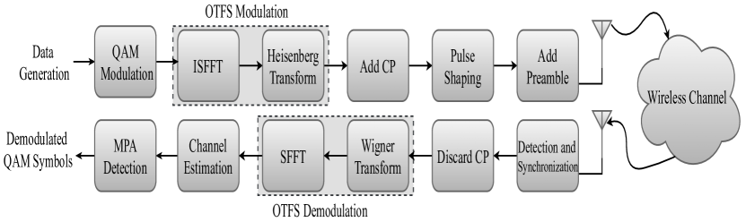
Figure 1: OTFS transceiver block diagram.

The main contributions of this paper are summarized is to present and emulates different RF-impairments at both transmitter and receiver when OTFS waveform is used for communication, and then, it compares these impairments to OFDM waveform. This work concentrate on major RF front-end impairments: PAPR, CFO, I/Q imbalance, DC-offset, and phase noise impairments. Testing and evaluation of the RF-impairments of the OTFS and OFDM waveforms are examined under real-time experiment using Keysight Agilent Technologies EXA signal analyzer N9010A [20].

I-C Organization

The remainder of this paper is organized as follows. Section II presents the modulation and demodulation of both OTFS and OFDM waveforms.

Section III discusses the channel effects and the RF-impairments impact, and shows the real implementation results. Finally, Section IV concludes the work.

II Waveform Modulation and Demodulation

The waveform is known as the physical shape of information represented by a signal transmitted through the channel. The transmitted signal $x(t)$ in a pulse-shaping system is formed by modulating data symbols $d_{n,k}$ onto time-frequency (Delay-Doppler) shifted versions of a transmit pulse $g(t)$ i.e.,

$$x(t)=\sum_{n\in\mathbb{Z}}\sum_{k\in\mathbb{Z}}d_{n,k}g_{n,k}(t),$$ (1)

with

$$g_{n,k}(t)=\left(\mathbb{M}_{kF}\mathbb{D}_{nT}g\right)(t)=g(t-nT)e^{j2\pi kFt},$$ (2)

where $\mathbb{M}_{\nu}\mathbb{D}_{\tau}$ is the time-frequency shift operator that includes a delay (time shift) $\tau=nT$ and a modulation (frequency shift) $\nu=kF$, $n$ is the time index, $k$ is the subcarrier index, $T$ is the sampling period, and $F$ is the sub-carrier spacing.

II-A OFDM Waveform

In OFDM systems, $N$ data symbols $X(k),k=0,1,...,N-1$ are mapped in the frequency domain i.e., $\mathbb{D}_{\tau}=0$. The pulse shaping filter $g(t)$ has a rectangular pulse shape in the transmitted lattice [21]. Then, by using (1), the transmitted OFDM discrete time-domain signal is given by

$$x[n]=\frac{1}{\sqrt{N}}\sum_{k=0}^{N-1}X(k)e^{j2\pi nk/N}.$$ (3)

The discrete signal expression of the $n$-th received sample is given as

$$y[n]=\frac{1}{\sqrt{N}}\sum_{k=0}^{N-1}H(k)X(k)e^{j2\pi n(k)/N}+w[n],$$ (4)

where ${H(k)}$ denotes the channel coefficients, and $w(n)$ is the zero-mean AWGN with $\sigma^{2}$ variance.

II-B OTFS Waveform

OTFS modulation is comprised of cascaded two-dimensional (2D) transforms at both transmitter and receiver, as shown in Fig. 1. At the transmitter side, the information symbols $X[l,k],k=0,...,N-1,l=0,...,M-1$ are map in the two-dimensional delay-Doppler domain from the modulation alphabet $\mathbb{A}$ to be transmit over $N.T$ time duration and using bandwidth $B=M.\Delta f$ . where $\Delta f=1/T$, and $N$, $M$ are the delay and Doppler bins, respectively.

Then inverse simplistic finite Fourier transform (ISFFT) using to map the $N\times M$ delay -Doppler grid points into the time-frequency (TF) plane as follows

$$x[n,m]=\frac{1}{NM}\sum_{k=0}^{N-1}\sum_{l=0}^{M-1}X[k,l]e^{j2\pi\left(\frac{nk}{N}-\frac{ml}{M}\right)}.$$ (5)

As illustrate by the dashed box in Fig. 1, the TF plane signal created is transformed to the time domain signal for transmission using the Heisenberg transform, which is given by [5, 6]

$$x(t)=\sum_{n=0}^{N-1}\sum_{m=0}^{M-1}X[n,m]g_{tx}(t-nT)e^{j2\pi m\Delta f(t-nT)}$$ (6)

where $g_{tx}$ denotes transmit pulse shaping. Unlike OFDM where CP is added for each of $N$ symbols in the frame, the CP is added for each frame in the time domain in OTFS. This considerably reduces the CP overhead. Then the signal will be transmitted through the time-varying wireless channel. The time domain received signal is expressed as

$$y(t)=\int_{\nu}\int_{\tau}h(\tau,\nu)x(t-\tau)e^{j2\pi\nu(t-\tau)}\mathrm{d}\tau\mathrm{d}\nu$$ (7)

where $\tau$ and $\nu$ denote the delay and Doppler variables, respectively. And $h(\tau,\nu)$ represent the complex channel response in delay Doppler domain. Wigner transform at the receiver side used to transform the time domain received signal $y(t)$ to TF domain, by matching it with the receiver pulse shaping $g_{rx}$. Assum that the transmit pulse shaping $g_{tx}$ and the receiver pulse shaping $g_{rx}$ satisfy bi-orthogonality conditions (The next section will addresses the situation in which the conditions are not satisfied) then the TF signal is given by [5, 6, 22]

$$Y[n,m]=H[n,m]X[n,m]+W[n,m]$$ (8)

where $W[n,m]$ is the additive white Gaussian noise (AWGN) and $H[n,m]$ is given by

$$H[n,m]=\int_{\tau}\int_{\nu}h(\tau,\nu)e^{j2\pi\nu nT}e^{-j2\pi(\nu+m\Delta f)\tau}\mathrm{d}\nu\mathrm{d}\tau$$ (9)

Then the symplectic finite Fourier transform (SFFT) is used to mapped the TF signal in delay-Doppler domain, which is defined as follows:

$$\hat{y}[k,l]=\frac{1}{NM}\sum_{n=0}^{N-1}\sum_{m=0}^{N}Y[n,m]e^{-j2\pi\left(\frac{nk}{N}-\frac{ml}{M}\right)}$$ (10)

$$=\frac{1}{NM}\sum_{n=0}^{N-1}\sum_{m=0}^{M-1}x[n,m]h(\tau^{^{\prime}},\nu^{^{\prime}})+w[k,l],$$

Message passing (MP) detection will be used after OTFS demodulation to detect the received symbols $\hat{x}[k,l]$ from the Delay Doppler mapped received signal $\hat{y}[k,l]$, as will be illustrated in the following subsection. This will be done so that the symbols can be extracted from the received signal.

II-C Channel Estimation and MP Detection

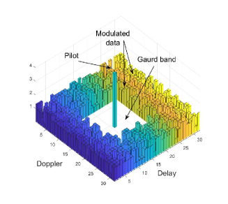
(a) Transmitted symbols.

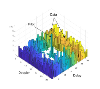
(b) Received signal.

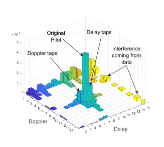
(c) Received embedded pilot.

Figure 2: The transmitted and received signal structure in the delay-Doppler plane.

At the receiver side, the doubly-dispersive channel response has to be estimated for the OTFS detection. In [23], the authors proposed a flag method to estimate the channel parameters and improved matched filter algorithm. However, the time-frequency domain estimate of the OTFS channels led to an increase in implementation complexity. In [24], MIMO-OTFS iterative algorithm was proposed for channel estimation in the delay-Doppler domain, where a whole OTFS frame containing pilots is used to estimate the channel. This estimation is used for next frame data detection. Unfortunately, this approach is valid only for time-invariant channels. In[25], embedded pilot-aided channel estimation scheme is proposed, where the receiver simultaneously proceeds a threshold approach channel estimation followed by message passing (MP) data detection in the same OTFS frame. Encouraged by the latter embedded pilot-aided estimation, in this paper, the OTFS frame is arranged as shown in Fig. 10 (a), where the data is distributed in the delay-Doppler domain. A guard band is adopted to prevent interference between the modulated data and the embedded pilot at the receiver detection as illustrated in Fig. 10 (b). Finally, the delay and Doppler taps (given in Fig. 10 (c)) are estimated and passed to the MP algorithm to detected the transmitted symbols.

After estimating the channel parameters, MP can be used to extract $\hat{x}[k,l]$ from the $\hat{y}[k,l]$ [24, 26, 27, 28] as it illustrate in algorithm 13. The detected received symbols are founded by evaluating the joint maximum a posteriori probability (MAP) represent as follows[29]:

$$\hat{x}=\underset{\mathbf{x}\in\mathbb{A}^{NM}}{\arg\max}\operatorname{Pr}({x}\mid{y},{H})$$ (11)

Adopting the same MAP detection in [29]. Let represent $y$ as a complex vector with element represents as $y[d]$ where $1\leq d\leq MN$ and $x$ is the information vector $x[c]$ where $1\leq c\leq MN$ and the complex channel will be represent as $H[d,c]$. Considering symbol by symbol detection $x_{c}$ and all the transmitted symbols $x_{c}\in\mathbb{A}$ have equivalently probability and independent form ${y}[d]$ , then $\hat{x}[c]$ is represent as

$$\hat{x}[c] =\underset{a_{j}\in\mathbb{A}}{\arg\max}\frac{1}{|\mathbb{A}|}\operatorname{Pr}\left(\mathrm{y}[d]\mid x[c]=a_{j},H[d,c]\right)$$ (12)

$$\approx\underset{a_{j}\in\mathbb{A}}{\arg\max}\prod_{d\in\mathcal{J}_{c}}\operatorname{Pr}\left(y[d]\mid x[c]=a_{j},H[d,c]\right)$$

In MAP detection, the observation node complex vector $y_{d}$, is related to the to variable node ${x_{e}},e\in\mathcal{I}_{d}$. Also, variable node $x_{c}$ are related to variable nodes ${y_{e}},e\in\mathcal{J}_{c}$. where $\mathcal{I}_{d}$, $\mathcal{J}_{c}$ represent positions of the $d^{th}$ rows and $c^{th}$ columns of the non zero element in $H$.

As it detailed in [29], massage is passing from observation nodes $y[d]$ to $x[c]$

$$y[d]=x[c]H[d,c]+\underbrace{\sum_{e\in\mathcal{I}(d),e\neq c}x[e]H[d,e]+w[d]}_{\zeta_{d,c}^{(i)}}$$ (13)

where $\zeta_{d,c}^{(i)}$ is represent the self interference that is could be approximate as Gaussian distribution according to central limit theorem (CLT) by evaluate the mean and variance. For more details see LABEL:y_detection [26, 27] [28] , where the approximated means and variance expressed as follow respectively[29]:

$$\mu^{(i)}_{d,c}=\mathbb{E}\left(\zeta_{d,c}^{(i)}\right)=\sum_{d\in\mathcal{J}_{c},e\neq c}h_{d,e}\sum_{j=1,j\neq i}^{\left|\mathbb{A}\right|}\mathbb{E}\left(a_{j}\right)$$ (14)

$$=\sum_{e\in\mathcal{I}_{d},e\neq c}\sum_{j=1}^{|\mathbb{A}|}p_{ed}^{(i)}\left(a_{j}\right)a_{j}H_{d,e}$$ (15)

$${\sigma^{(i)}_{d,c}}^{2}=\sum_{e\in\mathcal{I}_{d},e\neq c}\left(\sum_{j=1}^{|\mathbb{A}|}p_{ed}^{(i)}\left(x_{j}\right)\left|x_{j}\right|^{2}\left|H_{d,e}\right|^{2}-\left|\mu_{i}\right|^{2}\right)$$ (16)

where the pmf $p_{cd}^{(i)}$ is evaluated as following

$$p_{cd}^{(i)}\left(x_{j}\right)=\Delta\cdot\tilde{p}_{cd}^{(i)}\left(x_{j}\right)+(1-\Delta)\cdot p_{cd}^{(i-1)}\left(x_{j}\right)$$ (17)

where $\Delta$ is the damping factor that determine the weight of the previous probability distribution to evaluate the next one and it value in range $0<\Delta\leq 1$ [30], and

$$\tilde{p}_{cd}^{(i)}\left(a_{j}\right)\propto\prod_{e\in\mathcal{J}_{c},e\neq d}\operatorname{Pr}\left(y_{e}\mid x_{c}=a_{j},\mathbf{H}\right)$$ (18)

where

$$\operatorname{Pr}\left(y_{e}\mid x_{c}=a_{j},\mathbf{H}\right)\propto\exp\left(\frac{-\left|y_{e}-\mu_{ec}^{(i)}-H_{e,c}a_{j}\right|^{2}}{\sigma_{ec}^{2,(i)}}\right)$$ (19)

The decisions made upon that symbols to be transmitted are set as follows:

$$\hat{x}_{c}=\underset{a_{j}\in\mathbb{A}}{\arg\max}p_{c}\left(a_{j}\right),\quad c\in\{0,\cdots,NM-1\}$$ (20)

where $p_{c}\left(a_{j}\right)=\prod_{e\in\mathcal{J}_{c}}\operatorname{Pr}\left(y_{e}\mid x_{c}=a_{j},\mathbf{H}\right)$

0:  Input parameters:$\textbf{H};\textbf{y};N;M;M_{mod};$and$n_{i}tr$;

0:  Initialization : $i=0$ and $\left|\mathbf{p}_{cd}^{(0)}=1/\right|\mathbb{A}\mid$ for $c=\{0,\cdots,NM-1\}$ and $d\in\mathcal{J}_{c}$ $\mu_{i}=0;\sigma^{2}_{i}=0;$

0:   Procedure:

1:  for  i=1:Length(iteration) do

2:     for  m=1:M  do

3:        for  n=1:N  do

3:           Compute and update$\mu_{mn}^{(i)};\left(\sigma_{mn}^{(i)}\right)^{2}$

4:        end for

5:     end for

6:     for  each $d\in\mathcal{J}_{c}$  do

6:        Compute$p_{cd}^{(i+1)}\left(a_{j}\right)=\Delta\cdot p_{cd}^{(i)}\left(a_{j}\right)+(1-\Delta)\cdot p_{cd}^{(i-1)}\left(a_{j}\right)$

6:        Compute $p_{cd}^{(i)}\left(a_{j}\right)\propto\prod_{e\in\mathcal{J}_{c},e\neq d}\operatorname{Pr}\left(y_{e}\mid x_{c}=a_{j},\mathbf{H}\right)$,

7:     end for

8:  end for

9:  if $\max_{c,d,a_{j}}\left|p_{cd}^{(i+1)}\left(a_{j}\right)-p_{cd}^{(i)}\left(a_{j}\right)\right|<\epsilon$ Or $i=i_{max}$ then

10:     Break

11:  else

12:     Go to step Procedure

13:  end if

13:  Outputs:

13:  $\hat{x}_{c}=\underset{a_{j}\in\mathbb{A}}{\arg\max}p_{c}\left(a_{j}\right),\quad c\in\{0,\cdots,NM-1\}$

Algorithm 1 MP detection

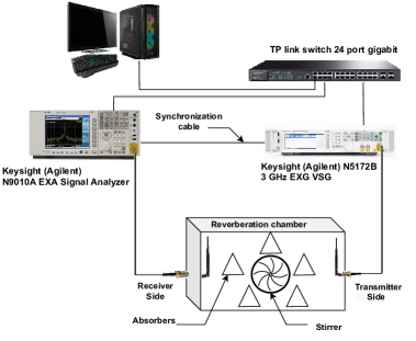
Figure 3: Laboratory equipment setup connection for multi-path emulation using Reverberation chamber.

III Channel Effects And RF-Impairments

The channel effect and the various RF-impairments degrade the system performance.Thus,in this section, the critical RF-impairments are discussed, and their effects on OFDM and OTFS are shown and compared experimentally. In the experiment platform, the SDR device based on the Keysight EXG X-Series design is used to implement terminals. As depicted in Fig. 4, the N5172B vector signal generator (VSG) with 9 kHz to 1, 3, or 6 GHz frequency range with output power +27 dBm, 900-µs switching speed. The receive antenna is connected to the N9010A EXA Keysight X-Series VSA [20]. Both the VSG and the signal analyzer are connected to the host PC running Matlab release 2020a software. The setup parameters are summarized in Table II.

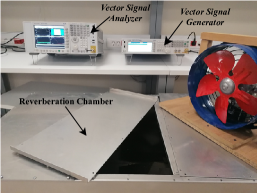
Figure 4: Laboratory equipment setup.

TABLE II: Simulation Parameters.

Symbol	Parameters	Value (OTFS)	Value (OFDM)
$f_{c}$	Carrier frequency	$2.4GHz,5GHz$ MHz	$2.4GHz,5GHz$
$M$	Number of subcarriers	$4,32,256$	$256,~{}1024$
$N$	Number of symbols	$4,32,256$	$1$
$T_{s}$	Symbol duration	$10~{}\mu s$
$M_{mod}$	Modulation order	QAM
$\Delta f_{s}$	Subcarrier spacing	$100$ KHz
$f_{o}$	Normalized frequency offset	$0,~{}0.05,~{}0.01,~{}0.1$
$\epsilon$	I/Q gain imbalance	$0\%,~{}50\%$
$\Delta\phi$	I/Q phase imbalance	$0^{o},~{}10^{o}$ degree

III-A Carrier frequency offset

In wireless communication, the propagating electromagnetic wave interacts with many obstacles called scatters, consequently, it is scattered, reflected, or refracted along with the propagation path. Therefore, for $L_{tap}$ different paths, $L_{tap}$ waves propagate with different delays and attenuation factors (i.e., multipath components). If the transmitter, receiver, or scatters are moving, these multipath components will be scaled in time equivalently causing a frequency shift (narrow-band) or frequency spreading (wide-band).

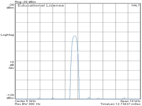
(a) Instantaneous spectrum stirrer-off

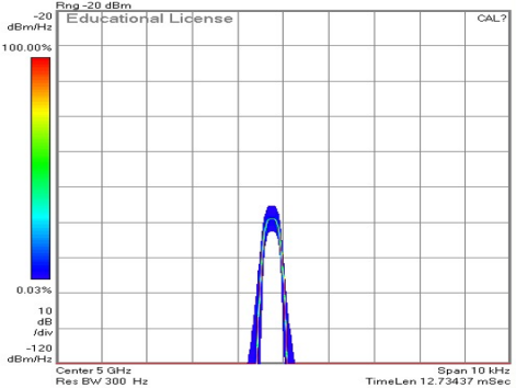
(b) Cumulative PSD when the stirrer-off

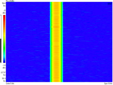
(c) Spectrogram when stirrer-off

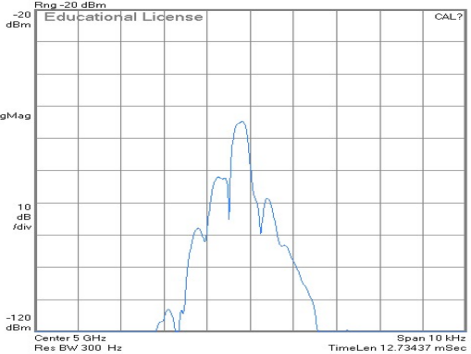
(d) Instantaneous spectrum stirrer-on.

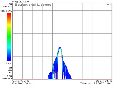
(e) Cumulative PSD when the stirrer-on

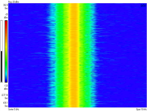
(f) Spectrogram when stirrer-on

Figure 5: Emulation the doppler shift effect on the 5GHz tone using reverberation chamber

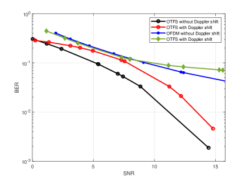
Figure 6: BER performance comparison between OTFS and OFDM effected by the Doppler shift using on the central frequency is 5GHz reverberation chamber.

Thus, Carrier frequency offset (CFO) is occurred due to either Doppler effects or carrier frequency mismatching between the TX and RX oscillators[31].Therefore, we will discuss both CFO effect in our experiment.

Firstly, In our setup, to create Doppler effect a metallic fan (stirrer) with $40cm\times 40cm\times 20cm$ dimensions with paddle radius of $0.15m$; is used creating Doppler shifts for high speed. In order to convert these shifts into Doppler spread, a reverberation chamber with the dimensions of $120cm\times 68cm\times 55cm$ is used to create more multi-path and provide enough Doppler spread for the experiment as shown in Fig. 3 [32].

Fig. 5 illustrates the Doppler spread when a 5GHz tone is transmitted before and after turning the stirrer with the highest speed. Before turning on the stirrer, it is seen that the received signal has a constant bandwidth over transmission time, however, as soon as the stirrer is turned on the spectrum enlarges taking up more bandwidth due to the spreading.

When the Doppler shift is generated, the BER performance of both the OTFS and OFDM waveforms degrades, as seen in the Fig.6. This degradation takes place as a result of the Doppler shift, which leads to the loss of orthogonality of the sub-carrier and eventually resulted in iter-carrier interference (ICI). However, as compared to OFDM waveform, OTFS waveform provides better BER performance. This is because the multipath components and Doppler shifts are resolvable in the delay-Doppler domain.

Assuming the resolved delays as $\tau_{i}$ and the Doppler frequency $\nu_{i}$, the received signal is given by the following weighted summation

$$y(t)=\sum_{i=1}^{L_{tap}}h_{i}x(t-\tau_{i})e^{j2\pi\nu_{i}t}=\sum_{i=1}^{L_{tap}}h_{i}\left(\mathbb{M}_{\nu_{i}}\mathbb{D}_{\tau_{i}}x\right)(t),$$ (21)

where $h_{i}$ is the $i$-th channel complex gain and $L_{tap}$ is the total number of resolvable paths.

Note that when using OTFS waveform, the multipath components and Doppler shifts are resolvable in the delay-Doppler domain, this is seen in Fig. 10 (c) where each bin represents a tap with specific delay and Doppler. This feature made the OTFS more suitable for rich scattering and high mobile environments than OFDM.

Now, different frequency offsets have been implemented in the N5172B-VSG in order to replicate the carrier frequency mismatching that occurs between the TX oscillator and the RX oscillator. owing to the fact that the frequency offset of the N5172B-VSG might be adjusted.

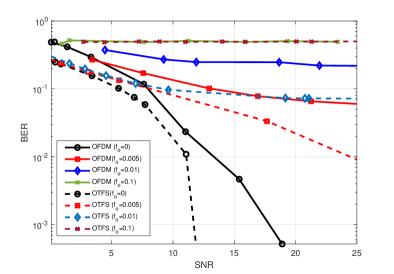
Figure 7: BER performance comparison between OTFS and OFDM systems with different normalized frequency offsets values in 2.4GHz carrier without using reverberation chamber.

The effect of the Doppler shifts caused by normalized frequency offsets may be seen in the BER performance of the OFDM and OTFS, which is presented in the Fig. 7. As can be seen in the figure, the BER performance of both the OTFS and OFDM waveforms decays when there is an increase in the value of the mismatching frequency offset. In addition to this, it was demonstrated that OTFS has superior performance in comparison to OFDM on consideration of the reasons that have been discussed previously.

III-B Non-linearity Impairments

Generally, there are different non-linearity sources in the RF front-end in communications systems namely, high power amplifier (HPA) at the transmitter, low-noise amplifier (LNA) at the receiver, mixtures, analog-to-digital (A/D) and digital-to-analog(D/A) converters[].

In real-world wireless communication systems, HPAs are the most commonly used component to provide long-distance wireless transmission. According to the non-linear input-output characteristic of HPAs, the power of the input signal should be amplified within the HPA’s linear range to prevent HPA to be saturated and cause the out-of-band (OOB) that degrades the system performance[]. The performance of the HPA amplifier is inversely proportional to the peak-to-average power ratio (PAPR) of the transmitted signal . As a result, the PAPR of the transmitted signal should be as minimal as possible [33].

The PAPR of the OTFS system is expressed as follow [34].

$${PAPR}=\frac{N\max_{k,l}|x[k,l]|^{2}}{\left.E\{\mid x[k,l]]^{2}\right\}}$$ (22)

Due to the fact that the PAPR is a random variable, the best way to measure and evaluate it is by using the complementary cumulative distribution function (CCDF) where the CCDF is presented as follows [34].

$$\operatorname{Pr}\left(PAPR>\gamma_{o}\right) =1-\operatorname{Pr}\left(PAPR\leq\gamma_{o}\right)$$ (23)

$$\approx 1-\left(1-e^{-\gamma_{o}}\right)^{MN}$$

where $Pr(.)$ denotes the probability function and $\gamma_{o}$ represents the threshold level that the PAPR of the transmitted OTFS signal should not exceed.

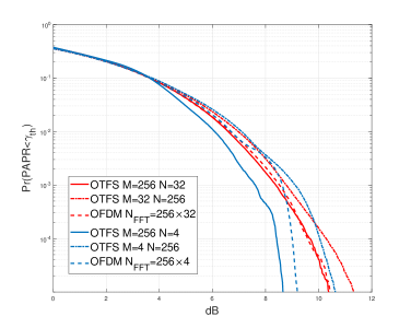
Figure 8: CCDF comparison of OTFS and OFDM.

Fig. 8 compares the CCDF of the PAPR for both OTFS and OFDM with the different values of $M$ and $N$ subcarriers. It is shown that for the same number of sub-carrier where $M>N$, OTFS provides better PAPR compared to OFDM. For example, for $M=256$ and $N=4$, OTFS has approximately 0.5 dB PAPR less than OFDM at the probability of $10^{-5}$. Also, it is observed that as $N$ increases the PAPR of the OTFS increases and the performance gap between the OTFS and OFDM almost vanishes. Note that in the case of $N>M$, it is shown that the PAPR of OTFS is the worst among all, this was discussed in detail in [15].

III-C I/Q Imbalance

In the communication system, direct-conversion receivers were used to convert radio frequency (RF) signals to base-band signals immediately. In contrast to heterodyne receivers, direct-conversion receivers did not need the signal to be down-converted to intermediate frequency (IF). Unfortunately, imperfections in the local oscillator (LO) might cause significant RF impairments, such I-Q imbalance and DC offset [35].

Local oscillator (LO) is a device that generates sine and cosine signals, which are used to represent in-phase and quadrature signals during the modulation and demodulation processes. To make a cosine signal, the LO produces a sine signal and shifts it $90^{\circ}$ degrees to produce a cosine signal. Unfortunately, the signal gain created and the phase $90^{\circ}$ are not in sync in terms of their practical implementation[31].

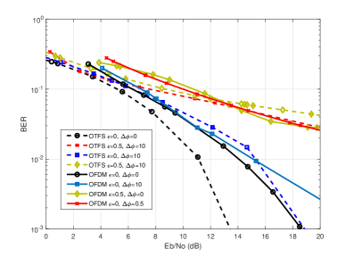
Figure 9: BER performance comparison between OTFS and OFDM systems with I/Q imbalances.

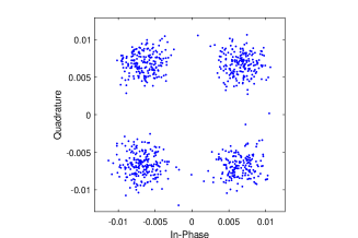
(a) $\epsilon=0,\Delta\phi=0$

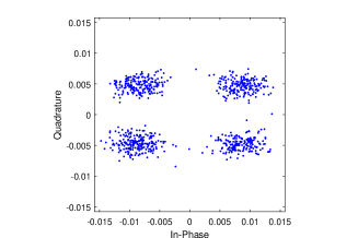
(b) $\epsilon=0,\Delta\phi=10$

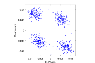
(c) $\epsilon=0.5,\Delta\phi=0$

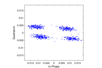
(d) $\epsilon=0.5,\Delta\phi=10$

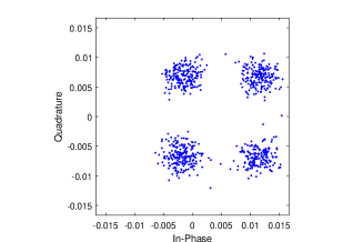
(e) $\gamma_{I}=0.75,\gamma_{Q}=0$

(f) $\gamma_{I}=0,\gamma_{Q}=0.75$

Figure 10: Constellation diagram shows the effect of the different IQ and DC offset on the 4-QAM constellation diagram.

I/Q imbalance impairment is the combination of two effects; the first one is the amplitude or gain imbalance (I) and the quadrature (Q) paths know as $\epsilon$, and the second one is the phase mismatch is given by $\Delta\phi$. The following model is used to add the I/Q imbalance on transmitted signal $x(t)=I+\jmath~{}Q$ [36, 37], as follows

$$y(t) =(1+\epsilon)\cos\Delta\phi\Re\{x(t)\}-\jmath(1-\epsilon)\sin\Delta\phi\Re\{x(t)\}$$ (24)

$$+\jmath(1-\epsilon)\cos\Delta\phi\Im\{x(t)\}-(1+\epsilon)\sin\Delta\phi\Im\{x(t)\},$$

where $\Re(\cdot)$ and $\Im(\cdot)$ symbolize the real and the imaginary part, respectively. For more simplicity, (24) could be written as

$$y(t)=\alpha\cdot x(t)+\beta\cdot x(t)^{*},$$ (25)

where $(\cdot)^{*}$ denote complex conjugate, $\alpha=\cos\Delta\phi+\jmath\epsilon\sin\Delta\phi$, and $\beta=\epsilon\cos\Delta\phi-\jmath\sin\Delta\phi$. As it is observed in (25) that the I/Q imbalance does not exist if $\alpha=1$ and $\beta=0$.

In the N5172B-VSG , there is a specification for an internal I/Q baseband generator that may be adjusted either internally or externally, depending on the application. In this experiment, we adjust the internal I/Q baseband of the N5172B-VSG to evaluate the effect of I/Q imbalance on the performance of the OTFS system.

Fig. 9 shows the effect of I/Q imbalance on the average BER performance for both OTFS and OFDM systems. In general, I/Q imbalance degrades the system’s performance for both waveforms as $\epsilon$ and/or $\Delta\phi$ increase, where as the I/Q imbalances are introduced in the system, the performance directly converges to a constant error floor at certain SNR value. Beyond this value, even increasing SNR does not help in improving the BER performance as given in [18].

Additionally, it can be seen that changing the value of gain $\epsilon$ causes a bad influence that is greater than that of $\Delta\phi$. This is because changing $\epsilon$ leads to narrowing the received symbols in constellations, which in turn leads to narrowing the thresholds regions’s that the demodulation should use to distinguish the received symbols. In other words, changing $\epsilon$ causes a more negative effect than changing $\Delta\phi$, Since the points in the constellation are now quite near to each other. While changing $\Delta\phi$ causes symbols to shift without changing on the distance between neighboring points.

III-D DC offset

The DC offset is also caused by the imperfection of the LO in direct-conversion receivers. where it is induced due to the leakage self-mixing of LO and transistor mismatch in the RF components[38]. DC offset will result in a shift on the symbols used in the constellation diagram (I/Q plane), and this shift might occur on the I-component, the Q-component, or both of them [35].

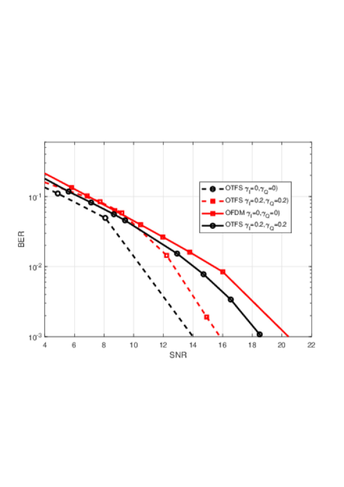
Figure 11: Comparison of the BER performance between OTFS and OFDM waveform

The comparison of the impact of the DC-offset on the BER performance of OTFS and OFDM is shown in the Fig.11, and it can be seen that the two waveforms have approximately the same influence on their BER performance. As was demonstrated, the effect of the DC-offset has a smaller impact on the system when the signal-to-noise ratio (SNR) is low, but it becomes more noticeable as the SNR rises. This is because the DC-offset expresses in the form of interference in the center of the transmission frequency spectrum, and as the SNR rises, the interference’s impact on the system’s overall performance accumulates.

The impact that varying values of the DC-offset have on the performance of the OTFS waveform is seen in Fig.12. According to the results, the degradation in system performance may be attributed to an increase in the DC-offset values. Additionally, it was shown that whether the in-phase DC-offset or the quadrature DC-offset, the system had the same influence on the performance of the system.

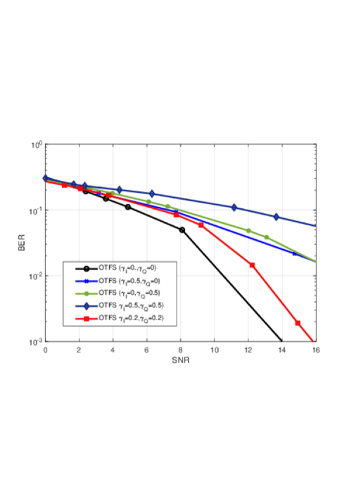
Figure 12: BER performance for OTFS under different values of DC-offset

III-E Phase noise

When a local oscillator in a transceiver is unable to create pure sinusoidal waves in conformance with the Dirac spectrum, phase noise is produced as shown in Fig.13 (a) and (b) . The frequency spectrum and timing properties of the oscillator output induce large adjustments as a direct result of PN’s influence [31].

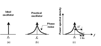
Figure 13: Phase noise of the local oscillator. (a) Ideal oscillator, (b) Practical oscillator, and (c) phase noise power level in dBc/Hz with $\Delta f$ offset

In most cases, designers typically define PN in the frequency domain, using a bandwidth of one Hz and an offset of one $\Delta f$ from the carrier [31]. The power of the PN signal throughout this bandwidth is normalized in relation to the power of the carrier in dBc/Hz unit as illustrated in Fig.13(c).

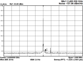
Figure 14: The phase noise of the VSA local oscillator

Both the N5172B vector signal generator (VSG) and the N9010A EXA Keysight X-Series vector signal analyzer (VSA) had amazingly low phase noise in our experiment.The phase noise of the VSA’s local oscillator is shown in Fig.14, According to what been seen, the phase noise of the local oscillator is equivalent to -137.06 dBm/Hz at 30Hz frequency offset.

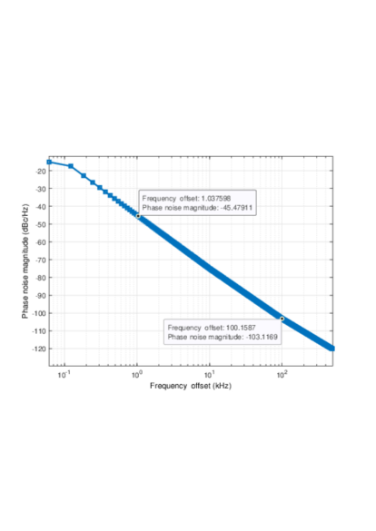
Figure 15:

The influence of phase noise will not be seen on the performance of the wave-forms systems because the level of phase noise is very low. Therefore, we have introduced phase noise at the receiver as illustrates Fig.15. And this modeling of the phase noise already exists on the 2.4GHz complementary metal-oxide-semiconductor voltage control oscillator (2.4GHz CMOS VCO) [39].

The phase noise impact on OTFS and OFDM BER performance is shown in Fig.16 Phase noise has been proven to have a detrimental effect on both the system’s performance and the orthogonality of the subcarriers, resulting in ICI. In contrast to OFDM, the OTFS waveform is more resistant to the phase noise effect.

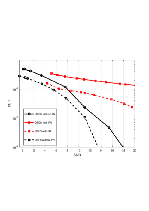
Figure 16: compersion of effect of the pahse noise on the BER performance for both OTFS and OFDM.

IV Conclusion

This paper emulates and compares the RF-impairments of the OTFS waveform to OFDM impairments using SDR. The experiments were conducted in a real indoor wireless environment, where the metallic structure of the building introduced enough multipath, the Doppler shift was induced by the Stirrer, and the impairments were inherently produced inside the devices or added before transmission. The BER performance of the OTFS modulation was superior than of the OFDM under doubly dispersive channel. The CCDF of the PAPR of OTFS is shown to vary with the lattice structure in the delay-Doppler domain, and under $M>N$ condition, OTFS provides better PAPR compare to OFDM. In addition, the I/Q-imbalance and DC-Offest impairments were explored, and the results showed that OTFS and OFDM are impacted in a manner that is approximately identical to one another. In addition, phase noise mitigation and OTFS give a higher level of phase noise resistance in comparison to OFDM. These findings provide an understanding of how and when to choose the waveform that is best appropriate for the characteristics of a particular channel.

Appendixes, if needed, appear before the acknowledgment.

References

- [1] C. V. N. Index, “Forecast and trends, 2017–2022 white paper,” Cisco Systems Inc.: San Jose, CA, USA, 2019.
- [2] Z. E. Ankarali, B. Peköz, and H. Arslan, “Flexible radio access beyond 5G: A future projection on waveform, numerology, and frame design principles,” IEEE Access, vol. 5, pp. 18 295–18 309, 2017.
- [3] A. M. Jaradat, J. M. Hamamreh, and H. Arslan, “Modulation options for OFDM-based waveforms: classification, comparison, and future directions,” IEEE Access, vol. 7, pp. 17 263–17 278, 2019.
- [4] S. Doğan-Tusha, H. Arslan et al., “6G Vision: An Ultra-Flexible Radio Access Technology Perspective,” arXiv preprint arXiv:2009.07597, 2020.
- [5] R. Hadani and A. Monk, “OTFS: A new generation of modulation addressing the challenges of 5G,” arXiv preprint arXiv:1802.02623, 2018.
- [6] R. Hadani, S. Rakib, M. Tsatsanis, A. Monk, A. J. Goldsmith, A. F. Molisch, and R. Calderbank, “Orthogonal time frequency space modulation,” in 2017 IEEE Wireless Communications and Networking Conference (WCNC). IEEE, 2017, pp. 1–6.
- [7] T. C. W. Schenk, “RF Impairments in Multiple Antenna OFDM: influence and mitigation,” 2006.
- [8] P. Raviteja, K. T. Phan, Y. Hong, and E. Viterbo, “Orthogonal time frequency space (otfs) modulation based radar system,” in 2019 IEEE Radar Conference (RadarConf), 2019, pp. 1–6.
- [9] L. Gaudio, M. Kobayashi, G. Caire, and G. Colavolpe, “On the effectiveness of otfs for joint radar parameter estimation and communication,” IEEE Transactions on Wireless Communications, vol. 19, no. 9, pp. 5951–5965, 2020.
- [10] Z. Ding, R. Schober, P. Fan, and H. Vincent Poor, “Otfs-noma: An efficient approach for exploiting heterogenous user mobility profiles,” IEEE Transactions on Communications, vol. 67, no. 11, pp. 7950–7965, 2019.
- [11] Y. Ge, Q. Deng, P. C. Ching, and Z. Ding, “Otfs signaling for uplink noma of heterogeneous mobility users,” IEEE Transactions on Communications, pp. 1–1, 2021.
- [12] R. Hadani, S. Rakib, A. F. Molisch, C. Ibars, A. Monk, M. Tsatsanis, J. Delfeld, A. Goldsmith, and R. Calderbank, “Orthogonal time frequency space (otfs) modulation for millimeter-wave communications systems,” in 2017 IEEE MTT-S International Microwave Symposium (IMS), 2017, pp. 681–683.
- [13] F. Wiffen, L. Sayer, M. Z. Bocus, A. Doufexi, and A. Nix, “Comparison of otfs and ofdm in ray launched sub-6 ghz and mmwave line-of-sight mobility channels,” in 2018 IEEE 29th Annual International Symposium on Personal, Indoor and Mobile Radio Communications (PIMRC), 2018, pp. 73–79.
- [14] G. D. Surabhi, M. K. Ramachandran, and A. Chockalingam, “Otfs modulation with phase noise in mmwave communications,” in 2019 IEEE 89th Vehicular Technology Conference (VTC2019-Spring), 2019, pp. 1–5.
- [15] G. Surabhi, R. M. Augustine, and A. Chockalingam, “Peak-to-average power ratio of OTFS modulation,” IEEE Communications Letters, vol. 23, no. 6, pp. 999–1002, 2019.
- [16] A. M. Jaradat, J. M. Hamamreh, and H. Arslan, “Generalized and flexible modulation options,” Flexible and Cognitive Radio Access Technologies for 5g and Beyond, p. 143, 2020.
- [17] S. Gao and J. Zheng, “Peak-to-average power ratio reduction in pilot-embedded otfs modulation through iterative clipping and filtering,” IEEE Communications Letters, vol. 24, no. 9, pp. 2055–2059, 2020.
- [18] S. G. Neelam and P. R. Sahu, “Error performance of otfs in the presence of iqi and pa nonlinearity,” in 2020 National Conference on Communications (NCC). IEEE, 2020, pp. 1–6.
- [19] T. Thaj and V. Emanuele, “OTFS Modem SDR Implementation and Experimental Study of Receiver Impairment Effects,” in 2019 IEEE International Conference on Communications Workshops (ICC Workshops). IEEE, 2019, pp. 1–6.
- [20] X. Keysight and S. S. Anayzers, “Keysight Technologies,” Santa Rosa, CA, USA, 2014.
- [21] A. Sahin, I. Guvenc, and H. Arslan, “A survey on multicarrier communications: Prototype filters, lattice structures, and implementation aspects,” IEEE communications surveys & tutorials, vol. 16, no. 3, pp. 1312–1338, 2013.
- [22] G. Surabhi and A. Chockalingam, “Low-complexity linear equalization for otfs modulation,” IEEE communications letters, vol. 24, no. 2, pp. 330–334, 2019.
- [23] A. Fish, S. Gurevich, R. Hadani, A. M. Sayeed, and O. Schwartz, “Delay-Doppler channel estimation in almost linear complexity,” IEEE Transactions on Information Theory, vol. 59, no. 11, pp. 7632–7644, 2013.
- [24] M. K. Ramachandran and A. Chockalingam, “MIMO-OTFS in high-Doppler fading channels: Signal detection and channel estimation,” in 2018 IEEE Global Communications Conference (GLOBECOM). IEEE, 2018, pp. 206–212.
- [25] P. Raviteja, K. T. Phan, and Y. Hong, “Embedded pilot-aided channel estimation for OTFS in delay–Doppler channels,” IEEE Transactions on Vehicular Technology, vol. 68, no. 5, pp. 4906–4917, 2019.
- [26] T. L. Narasimhan and A. Chockalingam, “Channel hardening-exploiting message passing (chemp) receiver in large-scale mimo systems,” IEEE Journal of selected topics in signal processing, vol. 8, no. 5, pp. 847–860, 2014.
- [27] Y. Ge, Q. Deng, P. Ching, and Z. Ding, “Receiver design for otfs with fractionally spaced sampling approach,” IEEE Transactions on Wireless Communications, 2021.
- [28] P. Raviteja, K. T. Phan, Q. Jin, Y. Hong, and E. Viterbo, “Low-complexity iterative detection for orthogonal time frequency space modulation,” in 2018 IEEE Wireless Communications and Networking Conference (WCNC). IEEE, 2018, pp. 1–6.
- [29] P. Raviteja, K. T. Phan, Y. Hong, and E. Viterbo, “Interference cancellation and iterative detection for orthogonal time frequency space modulation,” IEEE Transactions on Wireless Communications, vol. 17, no. 10, pp. 6501–6515, 2018.
- [30] M. Pretti, “A message-passing algorithm with damping,” Journal of Statistical Mechanics: Theory and Experiment, vol. 2005, no. 11, p. P11008, 2005.
- [31] A. Mohammadian and C. Tellambura, “Rf impairments in wireless transceivers: Phase noise, cfo, and iq imbalance–a survey,” IEEE Access, vol. 9, pp. 111 718–111 791, 2021.
- [32] A. B. Kihero, M. Karabacak, and H. Arslan, “Emulation techniques for small scale fading aspects by using reverberation chamber,” IEEE Transactions on Antennas and Propagation, vol. 67, no. 2, pp. 1246–1258, 2018.
- [33] M. Hossain, Y. Sugiura, T. Shimamura, H.-G. Ryu et al., “Dft-spread otfs communication system with the reductions of papr and nonlinear degradation,” Wireless Personal Communications, vol. 115, no. 3, pp. 2211–2228, 2020.
- [34] G. Surabhi, R. M. Augustine, and A. Chockalingam, “Peak-to-average power ratio of otfs modulation,” IEEE Communications Letters, vol. 23, no. 6, pp. 999–1002, 2019.
- [35] C.-H. Yih, “Analysis and compensation of dc offset in ofdm systems over frequency-selective rayleigh fading channels,” IEEE transactions on vehicular technology, vol. 58, no. 7, pp. 3436–3446, 2009.
- [36] B. Come, R. Ness, S. Donnay, L. Van der Perre, W. Eberle, P. Wambacq, M. Engels, and I. Bolsens, “Impact of front-end non-idealities on bit error rate performance of WLAN-OFDM transceivers,” in RAWCON 2000. 2000 IEEE Radio and Wireless Conference (Cat. No. 00EX404). Ieee, 2000, pp. 91–94.
- [37] J. Tubbax, B. Côme, L. Van der Perre, L. Deneire, S. Donnay, and M. Engels, “Compensation of IQ imbalance in OFDM systems,” in IEEE International Conference on Communications, 2003. ICC’03., vol. 5. IEEE, 2003, pp. 3403–3407.
- [38] S. G. Neelam and P. Sahu, “Analysis, estimation and compensation of hardware impairments for cp-otfs systems,” IEEE Wireless Communications Letters, 2022.
- [39] W. Yan and C. H. Park, “Filtering technique to lower phase noise for 2.4 ghz cmos vco,” in 2008 9th International Conference on Solid-State and Integrated-Circuit Technology. IEEE, 2008, pp. 1649–1652.