GWFAST: a Fisher information matrix Python code for third–generation gravitational–wave detectors

Abstract

We introduce GWFAST  , a Fisher information matrix Python code that allows easy and efficient estimation of signal–to–noise ratios and parameter measurement errors for large catalogs of resolved sources observed by networks of gravitational–wave detectors. In particular, GWFAST includes the effects of the Earth’s motion during the evolution of the signal, supports parallel computation, and relies on automatic differentiation rather than on finite differences techniques, which allows the computation of derivatives with accuracy close to machine precision. We also release the library WF4Py   implementing state–of–the–art gravitational–wave waveforms in Python. In this paper we provide a documentation of GWFAST and WF4Py with practical examples and tests of performance and reliability. In the companion paper Iacovelli et al. (2022) we present forecasts for the detection capabilities of the second and third generation of ground–based gravitational–wave detectors, obtained with GWFAST.

tablenum SIXtablenum

ET-0142A-22

1 Outline

GWFAST is a new, fast and accurate software, capable of computing signal–to–noise ratios (SNRs) and parameter measurement errors for networks of gravitational–wave (GW) detectors, using the Fisher Information Matrix (FIM) formalism. This approximates the full posterior probability distribution for the parameters of a GW signal (see e.g. Cutler & Flanagan (1994); Vallisneri (2008); Rodriguez et al. (2013) for a comprehensive treatment) and is used for forecasts on large catalogs of sources for which a full parameter estimation would be computationally too expensive. The computational cost is the main limitation of present–day forecast studies, especially for the third generation of GW detectors. This is related to two main aspects. The first is the duration of the signal (in particular, for binary neutron stars at ground–based detectors), which requires to correctly account for the time evolution of the antenna pattern functions and makes the data analysis challenging in terms of computational resources. To our knowledge, the problem of a full Bayesian inference for even a single one of such events is not manageable with techniques and resources used for second–generation (2G) detectors. Only recently dedicated approaches have started to be investigated (Smith et al., 2021). The second aspect is the scalability to large catalogs. The study of the reach and parameter estimation capabilities of third–generation (3G) detectors is a key aspect for assessing their scientific potential, and typically requires to study catalogs of tens of thousands of sources. GWFAST is suitable for these applications since it accounts for state–of–the–art waveform models, the effect of the motion of the Earth, and the possibility of parallel evaluations when running on large catalogs. Moreover, it does not rely on finite difference techniques to compute derivatives, but on automatic differentiation, which is a method that does not suffer from possible inaccuracies arising from the computation of the derivatives, in particular related to the choice of the step size. Hence we make it publicly available, together with routines to run in parallel. In this paper we provide a documentation, tests to validate the reliability of the code, and some examples. A scheme of the organization of the code is reported in Fig. 1. In the companion paper Iacovelli et al. (2022) we used GWFAST to produce forecasts for the detection capabilities of LIGO–Virgo–KAGRA (LVK) during their forthcoming O4 run, and of 3G ground–based GW detectors, namely, Einstein Telescope (ET) and Cosmic Explorer (CE), based on up–to–date models of the expected population of sources.

This paper is structured as follows. In Sect. 2 we describe the conventions for the input parameters and the waveform models available in GWFAST, which are a pure Python version of those contained in the LIGO Algorithm Library LAL (LIGO Scientific Collaboration, 2018), and compare with their original implementation. The waveform models are also separately released in a ready–to–use version, WF4Py. Moreover, GWFAST implements an interface with LAL, so that all the waveforms available in this library can be used directly. Only the use of the pure Python implementation allows however to fully exploit the vectorization capabilities of GWFAST and the use of automatic differentiation, as explained below. In Sect. 3 we document the two core modules of the software: signal and network, which allow the user to easily compute SNRs and FIMs, with various code examples. In particular, in Sect. 3.3 we provide an overview of how GWFAST deals with the computation of the derivatives of the signal with respect to the parameters. If using the Python implementation of the waveforms, we evaluate those using the automatic differentiation module of the JAX library (Bradbury et al., 2018), which ensures a fast and accurate computation, while if using the LAL waveforms the computation is performed using finite differences techniques. In Sect. 4 we then describe how GWFAST deals with the inversion of the Fisher matrix, to obtain the covariance matrix and thus the measurement errors, and the various manipulations that can be performed using the module fisherTools. Sect. 5 is devoted to the description of how to run GWFAST on multiple CPUs, so to easily handle huge catalogs of events, through the module calculate_forecasts_from_catalog.py. Finally in Sect. 6, to assess its reliability, we show the application of GWFAST to some of the real events observed by the LIGO and Virgo interferometers during their second and third observing runs, for which a full Bayesian parameter estimation has been performed. In Sect. 7 we then summarise and conclude.

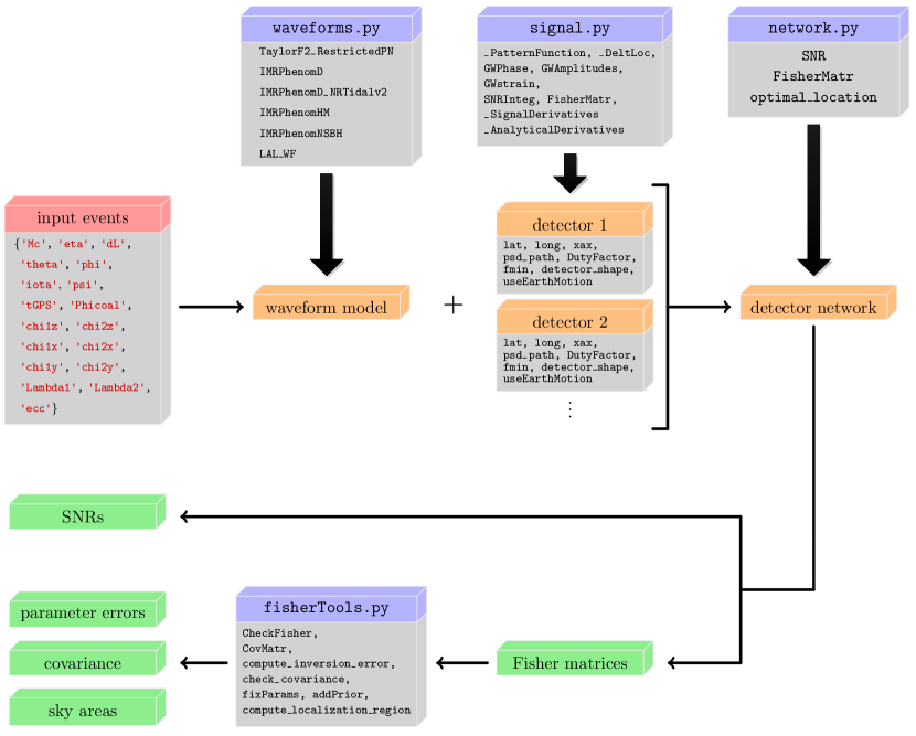
Figure 1: Flowchart of the functioning of GWFAST. See Sect. 2.1 for the description of the inputs.

2 Signal modelling

Waveform models give the prediction for a GW signal emitted by a coalescing binary as a function of the parameters of the source. We here give a brief overview of the chosen conventions for these parameters, as well as the waveforms available in GWFAST and their implementation.

2.1 Input parameters

In the most general case, restricting to quasi–circular orbits, the parameters needed to describe the signal emitted by a coalescing binary system are 15 for a binary black hole (BBH), 17 for a binary neutron star (BNS) and 16 for a neutron star black hole binary (NSBH), i.e. ${\bf\it\theta}=\{{\cal M}_{c},\eta,d_{L},\theta,\phi,\iota,\psi,t_{c},\Phi_{c},\chi_{1,x},\chi_{2,x},\chi_{1,y},\chi_{2,y},\chi_{1,z},\chi_{2,z},\Lambda_{1},\Lambda_{2}\}$ (see e.g. Maggiore (2007)), where: ${\cal M}_{c}$ denotes the detector–frame chirp mass, $\eta$ the symmetric mass ratio, $d_{L}$ the luminosity distance to the source, $\theta$ and $\phi$ are the sky position coordinates, defined as $\theta=\pi/2-\delta$ and $\phi=\alpha$ (with $\alpha$ and $\delta$ right ascension and declination, respectively), $\iota$ the inclination angle of the binary orbital angular momentum with respect to the line of sight, $\psi$ the polarisation angle, $t_{c}$ the time of coalescence, $\Phi_{c}$ the phase at coalescence, $\chi_{i,c}$ the dimensionless spin of the object $i=\{1,2\}$ along the axis $c=\{x,y,z\}$ and $\Lambda_{i}$ the dimensionless tidal deformability of the object $i$, which is zero for a BH. GWFAST expresses the chirp mass in units of solar masses, $\mathrm{M_{\odot}}$, the luminosity distance in $\mathrm{Gpc}$, the time of coalescence as a GPS time, in seconds, and all the angles in radiants. Including also a small eccentricity in the orbit, there is one more parameter to consider, $e_{0}$, which denotes the eccentricity at a given reference frequency.

To use GWFAST, the parameters ${\bf\it\theta}$ of the events in the catalog to analyse have to be stored in a dictionary, with the same keys as in the following example

⬇

import numpy as np

events = {'Mc':np.array([...]), 'eta':np.array([...]), 'dL':np.array([...]),

'theta':np.array([...]), 'phi':np.array([...]), 'iota':np.array([...]),

'psi':np.array([...]), 'tGPS':np.array([...]), 'Phicoal':np.array([...]),

'chi1z':np.array([...]), 'chi2z':np.array([...]),

'chi1x':np.array([...]), 'chi2x':np.array([...]),

'chi1y':np.array([...]), 'chi2y':np.array([...]),

'Lambda1':np.array([...]), 'Lambda2':np.array([...]), 'ecc':np.array([...])

}

Code example 1: Input parameters for waveform models and FIM calculations in GWFAST.

It is also possible to pass some entries with different commonly used parametrizations, namely:

1. the sky position coordinates can be given in terms of right ascension $\alpha$ and declination $\delta$, always in radiants, in place of $\theta$ and $\phi$;

2. the time of coalescence can be provided as a Greenwich Mean Sidereal Time (GMST) in days, under the entry name 'tcoal', which takes the place of 'tGPS';

3. in the non precessing case, one can choose the spin parameters $\chi_{s},\chi_{a}$ instead of $\chi_{1,z},\chi_{1,z}$, defined as

   $$\chi_{s}=\dfrac{1}{2}(\chi_{1,z}+\chi_{2,z})\,,\qquad\chi_{a}=\dfrac{1}{2}(\chi_{1,z}-\chi_{2,z})\,;$$ (1)

4. it is possible to use the combinations of the tidal deformabilities $\tilde{\Lambda},\delta\tilde{\Lambda}$ in place of $\Lambda_{1},\Lambda_{2}$, whose definitions are (Wade et al., 2014)

   $$\tilde{\Lambda} =\dfrac{8}{13}\left[(1+7\eta-31\eta^{2})(\Lambda_{1}+\Lambda_{2})+\sqrt{1-4\eta}(1+9\eta-11\eta^{2})(\Lambda_{1}-\Lambda_{2})\right]\,,$$ (2a)

   $$\delta\tilde{\Lambda} =\dfrac{1}{2}\left[\sqrt{1-4\eta}\left(1-\dfrac{13272}{1319}\eta+\dfrac{8944}{1319}\eta^{2}\right)(\Lambda_{1}+\Lambda_{2})+\left(1-\dfrac{15910}{1319}\eta+\dfrac{32850}{1319}\eta^{2}+\dfrac{3380}{1319}\eta^{3}\right)(\Lambda_{1}-\Lambda_{2})\right]\,;$$ (2b)

5. if using a waveform model which includes the contribution of unaligned spin components (precessing spins) it is possible to substitute the entries $\iota,\chi_{1,x},\chi_{2,x},\chi_{1,y},\chi_{2,y},\chi_{1,z},\chi_{2,z}$ with $\theta_{JN},\chi_{1},\chi_{2},\theta_{s,1},\theta_{s,2},\phi_{JL},\phi_{1,2}$. These are, respectively, the angle between the total angular momentum and the line of sight, $\theta_{JN}$, the magnitudes of the spin vectors, $\chi_{i}$, the angles between the spin vectors and the orbital angular momentum, $\theta_{s,i}$, the azimuthal angle of the orbital angular momentum and the total angular momentum, $\phi_{JL}$, and the difference in azimuthal angle between the two spin vectors, $\phi_{1,2}$.

A summary of the parameters, their physical symbol and their name in GWFAST is provided in Tab. 1.

parameter symbol	parameter description	name in GWFAST	units in GWFAST	physical range
${\cal M}_{c}$	detector–frame chirp mass	'Mc'	$\mathrm{M_{\odot}}$	$(0,\,+\infty)$
$\eta$	symmetric mass ratio	'eta'	–	$(0,\,0.25]$
$d_{L}$	luminosity distance	'dL'	$\mathrm{Gpc}$	$(0,\,+\infty)$
$\theta$, $\phi$ / $\alpha$, $\delta\,^{\rm\ref{item:inp_radec}}$	sky position	'theta', 'phi' /	rad	$[0,\,\pi]$, $[0,\,2\pi]$ /
		'ra', 'dec'		$[0,\,2\pi]$, $[-\pi/2,\,\pi/2]$
$\iota\,^{\rm\ref{item:inp_prec}}$	inclination angle w.r.t. orbital	'iota'	rad	$[0,\,\pi]$
	angular momentum
$\psi$	polarisation angle	'psi'	rad	$[0,\,\pi]$
$t_{c}\,^{\rm\ref{item:inp_tc}}$	time of coalescence GPS / GMST	'tGPS' / 'tcoal'	s / day	$[0,\,+\infty)$ / $[0,\,1]$
$\Phi_{c}$	phase at coalescence	'Phicoal'	rad	$[0,\,2\pi]$
$\chi_{i,c}\,^{\rm\ref{item:inp_chiSA},\,\ref{item:inp_prec}}$	spin component of object $i=\{1,2\}$	'chi1x', 'chi1y', 'chi1z'	–	$[-1,\,1]$, ($S^{2}$)
	along axis $c=\{x,y,z\}$	'chi2x', 'chi2y', 'chi2z'
$\Lambda_{i}\,^{\rm\ref{item:inp_LamT}}$	adimensional tidal deformability	'Lambda1', 'Lambda2'	–	$[0,\,+\infty)$
	of object $i=\{1,2\}$
$e_{0}$	orbital eccentricity	'ecc'	–	$[0,\,1)$
$\chi_{s}$, $\chi_{a}\,^{\rm\ref{item:inp_chiSA}}$	symmetric and asymmetric spin	'chiS', 'chiA'	–	$[-1,\,1]$, $[-1,\,1]$
	components, see Eq. (1)
$\tilde{\Lambda}$, $\delta\tilde{\Lambda}\,^{\rm\ref{item:inp_LamT}}$	adimensional tidal deformability	'LambdaTilde',	–	$[0,\,+\infty)$,
	combinations, see Eq. (2)	'deltaLambda'		$(-\infty,\,+\infty)$
$\theta_{JN}\,^{\rm\ref{item:inp_prec}}$	inclination angle w.r.t. total	'thetaJN'	rad	$[0,\,\pi]$
	angular momentum
$\chi_{i}\,^{\rm\ref{item:inp_prec}}$	spin magnitude of object $i=\{1,2\}$	'chi1', 'chi2'	–	$[0,\,1]$
$\theta_{s,i}\,^{\rm\ref{item:inp_prec}}$	spin tilt of object $i=\{1,2\}$	'tilt1', 'tilt2'	rad	$[0,\,\pi]$
$\phi_{JL}\,^{\rm\ref{item:inp_prec}}$	azimuthal angle between orbital	'phiJL'	rad	$[0,\,2\pi]$
	and total angular momentum
$\phi_{1,2}\,^{\rm\ref{item:inp_prec}}$	difference in azimuthal angle	'phi12'	rad	$[0,\,2\pi]$
	between the spin vectors

Table 1: Summary of the parameters used in GWFAST to describe the GW signal. The first column reports the symbol used to denote a parameter, the second a brief description of its physical meaning, the third its name in GWFAST, the fourth the physical units of the parameter adopted in GWFAST and the last its physical range. Parameters describing the same physical quantities, which thus have to be provided alternatively, are followed by a superscript in the first column, matching the one reported in the list in Sect. 2.1. $S^{2}$ in the $\chi_{i,c}$ stresses that the 3 components of a spin vector are not independent, but defined on a sphere, i.e. $\chi_{i,x}^{2}+\chi_{i,y}^{2}+\chi_{i,z}^{2}\leq 1$.

2.2 Waveform models

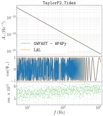
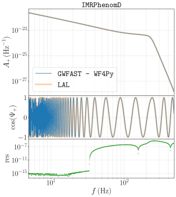
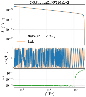
(a) Parameters: ${\cal M}_{c}=$1.65\text{\,}\mathrm{M_{\odot}}$,\ \eta=0.25,$	(b) Parameters: ${\cal M}_{c}=$36\text{\,}\mathrm{M_{\odot}}$,\ \eta=0.24,$	(c) Parameters: ${\cal M}_{c}=$1.32\text{\,}\mathrm{M_{\odot}}$,\,\eta=0.25,$
$d_{L}=$0.46\text{\,}\mathrm{Gpc}$,\ \chi_{1}=0.05,\ \chi_{2}=-0.05,$	$d_{L}=$0.98\text{\,}\mathrm{Gpc}$,\ \chi_{1}=0.8,\ \chi_{2}=-0.8$.	$d_{L}=$0.46\text{\,}\mathrm{Gpc}$,\ \chi_{1}=0.05,\ \chi_{2}=0,$
$\Lambda_{1}=300,\ \Lambda_{2}=300$.		$\Lambda_{1}=500,\ \Lambda_{2}=500$.

Figure 2: Comparison of the waveform models TaylorF2_RestrictedPN (left panel), IMRPhenomD (central panel) and IMRPhenomD_NRTidalv2 (right panel) obtained from LAL and GWFAST – WF4Py for example events. The upper and central panel of both figures show the ‘+’ GW amplitude and cosine of the phase obtained with the two codes superimposed, while in the lower we report the relative difference (“residual”) among the two amplitudes.

We use Fourier domain waveform models. In particular, at the time of writing the code implements some selected waveform models in Python, and an interface to the LIGO Algorithm Library, LAL, which allows to use all the waveforms available in that library.
In particular, the following waveform models are directly available in GWFAST in a Python implementation:

TaylorF2_RestrictedPN

a restricted PN waveform model (Buonanno et al., 2009; Ajith, 2011; Mishra et al., 2016), also with its tidal (Wade et al., 2014) and moderate eccentric (Moore et al., 2016) extensions. This is an inspiral–only waveform, but can still be used to describe signals coming from BNS mergers, whose major contribution to the SNR comes from the inspiral. There is no limitation in the parameters range, except for the eccentricity, which cannot exceed $e_{0}\sim 0.1$ for comparable mass systems;

IMRPhenomD

a full inspiral–merger–ringdown waveform model (Husa et al., 2016; Khan et al., 2016), tuned with NR simulations, which can efficiently be used to simulate signals coming from BBH mergers, with non–precessing spins up to $|\chi_{z}|\sim 0.85$ and mass ratios up to $q=m_{1}/m_{2}\sim 18$;

IMRPhenomD_NRTidalv2

tidal extension of the previous model (Dietrich et al., 2019) which can be used to accurately describe signals coming from BNS mergers. It includes spin terms up to higher order and a filter to terminate the waveform after merger. The validity has been assessed for masses ranging from 1 to $3\text{\,}\mathrm{M_{\odot}}$, spins up to $|\chi_{z}|\sim 0.6$ and tidal deformabilities up to $\Lambda_{i}\simeq 5000$;

IMRPhenomHM

full inspiral–merger–ringdown waveform model (London et al., 2018; Kalaghatgi et al., 2020), which takes into account not only the quadrupole of the signal, but also the sub–dominant multipoles $(l,m)=(2,1),\ (3,2),\ (3,3),\ (4,3),\ {\rm and}\ (4,4)$, that can be particularly relevant to better describe the signal coming from BBH systems. The calibration range is the same of the IMRPhenomD model;

IMRPhenomNSBH

full inspiral–merger–ringdown waveform model (Pannarale et al., 2015; Dietrich et al., 2019), which can describe the signal coming from the merger of a NS and a BH, with mass ratios up to $q\sim 100$, also taking into account tidal effects and the impact of the possible tidal disruption of the NS.

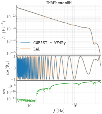
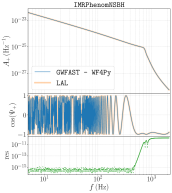
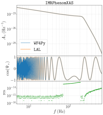
(a) Parameters: ${\cal M}_{c}=$44\text{\,}\mathrm{M_{\odot}}$,\ \eta=0.24,$	(b) Parameters: ${\cal M}_{c}=$3.85\text{\,}\mathrm{M_{\odot}}$,\ \eta=0.08,$	(c) Parameters: ${\cal M}_{c}=$36\text{\,}\mathrm{M_{\odot}}$,\ \eta=0.24,$
$d_{L}=$0.46\text{\,}\mathrm{Gpc}$,\ \chi_{1}=0.8,\ \chi_{2}=0.8$.	$d_{L}=$0.46\text{\,}\mathrm{Gpc}$,\ \chi_{1}=0.3,\ \chi_{2}=0,$	$d_{L}=$0.98\text{\,}\mathrm{Gpc}$,\ \chi_{1}=0.8,\ \chi_{2}=-0.8$.
	$\Lambda_{1}=0,\ \Lambda_{2}=400$.

Figure 3: As in Fig. 2 for the waveform models IMRPhenomHM (left panel), IMRPhenomNSBH (central panel) and IMRPhenomXAS (right panel).

These waveform models have been translated from their C implementation in the LIGO Algorithm Library, LAL, into a pure Python version. We carefully checked that our Python implementation accurately reproduces the original LAL waveforms, as can be seen on some example events in Fig. 2 and 3.

The implementation in Python has two advantages. First, it allows GWFAST to fully exploit the capabilities of this language to vectorize the computation on multiple events at a time, which would be impossible if we had to interact with a code written in C such as LAL. Second, it allows the possibility of using automatic differentiation (and in particular the library JAX) to compute derivatives, see Sect. 3.3.

It is also possible to use the waveform module separately from the rest of the code. For example, in order to generate the IMRPhenomD waveform amplitude and phase for a given set of events it is sufficient to run the following sequence of commands

⬇

import waveform as wf

# initialise the waveform, here we choose as an example IMRPhenomD

mywf = wf.IMRPhenomD()

# compute the cut frequencies

fcut = mywf.fcut(**events)

# initialise the frequency grids from 2Hz to fcut, with 1000 points per grid

fgrids = np.geomspace(np.full(fcut.shape, 2), fcut, num=1000)

# compute the amplitude and phase, respectively

myampl = mywf.Ampl(fgrids, **events)

myphase = mywf.Phi(fgrids, **events)

Code example 2: Calculation of waveforms in GWFAST and WF4Py. As an illustration, we use the IMRPhenomD model.

This small piece of code shows that, being GWFAST’s waveforms written in pure Python and fully vectorized, our software does not have to rely on for loops over the events, as in a code interacting with C. Note that the order of the entries in the events dictionary is arbitrary.

All our waveforms also include a routine to compute the time to coalescence as a function of frequency, needed to take into account Earth’s rotation in the computation of the strain, which includes terms up to 3.5 PN order, called tau_star, and a function to compute the cut frequency for the given waveform, so to properly build the frequency grid, called fcut, as seen in the above example. Waveforms objects in GWFAST contain the attribute ParNums giving a dictionary of the form {'name_of_parameter':position}, with 'name_of_parameter' being a string with the parameter name as in Tab. 1 and position being an int corresponding to the position of the parameter in the Fisher matrix.

Apart from their implementation in GWFAST, which includes some features specific for JAX compatibility, we publicly release a pure numpy and ready–to–use version of the waveform models alone, WF4Py . The syntax for using waveforms in this library is the same as in the example above. This module further implements the waveform model IMRPhenomXAS (Pratten et al., 2020), which is a full inspiral–merger–ringdown model tuned for the fundamental mode of BBH systems with aligned spins and mass ratios ranging from 1 to 1000, among the last to be released.

Finally, all waveform models available in LAL can be accessed in GWFAST through the wrapper class LAL_WF, which can be used as follows

⬇

myLALwf = wf.LAL_WF('IMRPhenomXPHM', is_tidal=False, is_HigherModes=True, is_Precessing=True, is_eccentric=False)

Code example 3: How to use LAL waveforms in GWFAST. As an illustration, we use the IMRPhenomXPHM model.

where the first entry has to be a string containing the name of the chosen waveform as in the LAL library  – 'IMRPhenomXPHM' in this example – and the Booleans is_tidal, is_HigherModes, is_Precessing and is_eccentric are used to specify whether the model includes tidal effects, the contribution of higher–order harmonics, precessing spins or eccentricity (see also footnote 3), respectively.

3 Detector response and Fisher Matrix

The core modules of GWFAST are signal and network. The former allows to model the response of a single detector to a GW signal, while the latter collects multiple detectors constituting a network. Both modules include in particular methods to compute the signal–to–noise ratio (SNR) and the FIM. GWFAST fully accounts for the motion of the Earth during the time the signal remains in the detection band, see Iacovelli et al. (2022) for a detailed discussion.

3.1 Single detector

Detector	latitude $\lambda$	longitude $\varphi$	orientation $\gamma$	arms aperture $\zeta$	shape	name in GWFAST
LIGO Hanford, USA	$46.5\text{\,}\mathrm{\SIUnitSymbolDegree}$	$-119.4\text{\,}\mathrm{\SIUnitSymbolDegree}$	$171\text{\,}\mathrm{\SIUnitSymbolDegree}$	$90\text{\,}\mathrm{\SIUnitSymbolDegree}$	'L'	'H1'
LIGO Livingston, USA	$30.6\text{\,}\mathrm{\SIUnitSymbolDegree}$	$-90.8\text{\,}\mathrm{\SIUnitSymbolDegree}$	$242.7\text{\,}\mathrm{\SIUnitSymbolDegree}$	$90\text{\,}\mathrm{\SIUnitSymbolDegree}$	'L'	'L1'
Virgo, Cascina, IT	$43.6\text{\,}\mathrm{\SIUnitSymbolDegree}$	$10.5\text{\,}\mathrm{\SIUnitSymbolDegree}$	$115.6\text{\,}\mathrm{\SIUnitSymbolDegree}$	$90\text{\,}\mathrm{\SIUnitSymbolDegree}$	'L'	'Virgo'
KAGRA, Hida, JP	$36.4\text{\,}\mathrm{\SIUnitSymbolDegree}$	$137.3\text{\,}\mathrm{\SIUnitSymbolDegree}$	$15.4\text{\,}\mathrm{\SIUnitSymbolDegree}$	$90\text{\,}\mathrm{\SIUnitSymbolDegree}$	'L'	'KAGRA'
LIGO India, Hingoli, IN	$19.6\text{\,}\mathrm{\SIUnitSymbolDegree}$	$77.0\text{\,}\mathrm{\SIUnitSymbolDegree}$	$287.4\text{\,}\mathrm{\SIUnitSymbolDegree}$	$90\text{\,}\mathrm{\SIUnitSymbolDegree}$	'L'	'LIGOI'
ET Sardinia, IT	$40.5\text{\,}\mathrm{\SIUnitSymbolDegree}$	$9.4\text{\,}\mathrm{\SIUnitSymbolDegree}$	$0\text{\,}\mathrm{\SIUnitSymbolDegree}$	$60\text{\,}\mathrm{\SIUnitSymbolDegree}$	'T'	'ETS'
ET Meuse–Rhine, EU	$50.7\text{\,}\mathrm{\SIUnitSymbolDegree}$	$5.9\text{\,}\mathrm{\SIUnitSymbolDegree}$	$0\text{\,}\mathrm{\SIUnitSymbolDegree}$	$60\text{\,}\mathrm{\SIUnitSymbolDegree}$	'T'	'ETMR'
CE1 Idaho, USA	$43.8\text{\,}\mathrm{\SIUnitSymbolDegree}$	$-112.8\text{\,}\mathrm{\SIUnitSymbolDegree}$	$-45\text{\,}\mathrm{\SIUnitSymbolDegree}$	$90\text{\,}\mathrm{\SIUnitSymbolDegree}$	'L'	'CE1Id'
CE2 New Mexico, USA	$33.2\text{\,}\mathrm{\SIUnitSymbolDegree}$	$-106.5\text{\,}\mathrm{\SIUnitSymbolDegree}$	$-105\text{\,}\mathrm{\SIUnitSymbolDegree}$	$90\text{\,}\mathrm{\SIUnitSymbolDegree}$	'L'	'CE2NM'
CE2 New South Wales, AU	$-34\text{\,}\mathrm{\SIUnitSymbolDegree}$	$145\text{\,}\mathrm{\SIUnitSymbolDegree}$	$0\text{\,}\mathrm{\SIUnitSymbolDegree}$	$90\text{\,}\mathrm{\SIUnitSymbolDegree}$	'L'	'CE2NSW'

Table 2: Summary of the positions, orientations, angle between arms, shapes and acronyms of the detectors available in GWFAST. Using user-defined configurations is straightforward (see the text). The orientation $\gamma$ denotes the angle between the bisector of the arms (the first arm in the case of a triangle) and East.

A signal object can be initialized from the class GWSignal as follows:

⬇

import signal

Virgo = signal.GWSignal(mywf, psd_path= 'path/to/Virgo/psd', detector_shape = 'L', det_lat=43.6, det_long=10.5, det_xax=115.)

LIGO_L = signal.GWSignal(mywf, psd_path= 'path/to/LIGO/L1/psd', detector_shape = 'L', det_lat=30.6, det_long=-90.8, det_xax=243.)

Code example 4: Initialization of objects characterising single detectors in GWFAST for a user–specified location, orientation, shape and path to the PSD file.

where det_lat and det_long denote the latitude and longitude of the detector in degrees, xax the angle between the bisector of the detector arms and the east in degrees, detector_shape its shape, which can be either 'L' (for L–shaped detectors) or 'T' (for triangular–shaped detectors). A triangular–shaped detector is defined as three co–located detectors with opening angle of $60\text{\,}\mathrm{\SIUnitSymbolDegree}$ in a closed–loop configuration.

Other options can be passed when initialising the GWSignal object, in particular: the useEarthMotion Boolean is used to turn on and off the computation of the effect of Earth’s rotation; fmin and fmax can be used to set the minimum and maximum of the frequency grid (in $\mathrm{Hz}$) and have default values fmin=2.0 and fmax=None (meaning that the grid extends up to the cut frequency of the waveform); DutyFactor can be used to set the duty factor of the detector, i.e. the fraction of time each detector is supposed to be operational, between 0 and 1 (default is None, meaning no duty cycle is considered). For triangular–shaped detectors, the duty factor refers to each of the three components of the triangle separately.

The entry psd_path is the path to the file containing its Amplitude Spectral Density (ASD) or Power Spectral Density (PSD) (the flag is_ASD can be used to specify whether the given one is a PSD or ASD). GWFAST contains the following publicly available ASDs in the folder data/psds/:

• the sensitivities from the study Abbott et al. (2017) (last update in January 2020), that can be found at https://dcc.ligo.org/LIGO-T1500293/public, in the folder unofficial_curves_all_dets;

• the representative sensitivities of the LIGO and Virgo detectors during the observing runs O1 and O2 (https://dcc.ligo.org/P1800374/public/), O3a (https://dcc.ligo.org/LIGO-P2000251/public) and O3b (estimated using PyCBC around the times reported in the caption of Fig. 2 of Abbott et al. (2021a)), in the folder LVC_O1O2O3;

• the sensitivities adopted in Abbott et al. (2020a) for the LIGO, Virgo and KAGRA detectors during the O3, O4 and O5 runs (https://dcc.ligo.org/LIGO-T2000012/public), in the folder observing_scenarios_paper;

• the official ET–D sensitivity curve, from the document ET-0000A-18.txt (https://apps.et-gw.eu/tds/?content=3&r=14065);

• the latest sensitivity curves for Cosmic Explorer, used in Srivastava et al. (2022), for various detector configurations (https://dcc.cosmicexplorer.org/CE-T2000017/public), in the folder ce_strain.

GWFAST also contains some pre–defined detector configurations in the module globals. These are listed, together with their acronyms, in Tab. 2. The locations of the current detectors are taken from Gossan et al. (2022), while the CE sites are taken from Borhanian (2021) as illustrative examples. Pre–defined detector configurations can be easily imported from globals. In the following, we show how to initialise one signal corresponding to one CE at the Hanford site, with orientation $\gamma=0$:

⬇

import copy

import os

import gwfastGlobals as glob

# copy the location and orientation of Hanford

CEH_conf = copy.deepcopy(glob.detectors).pop('H1')

# set the detector PSD using the latest curve for CE1

CEH_conf['psd_path'] = os.path.join(glob.detPath, 'ce_strain', 'cosmic_explorer.txt')

# Set the orientation angle to 0

CEH_conf['xax'] = 0

# Initialise the GWSignal object

CEH = signal.GWSignal(mywf, psd_path=CEH_conf['psd_path'], detector_shape=CEH_conf['shape'], det_lat=CEH_conf['lat'], det_long=CEH_conf['long'], det_xax=CEH_conf['xax'])

Code example 5: Initialization of objects characterising single detectors in GWFAST using pre–defined detector configurations.

Any other user–defined configuration can easily be added as in 4. With the object of type GWSignal initialized, the user can easily compute all the quantities characterising signal. In particular, from the _PatternFunction function it is possible to get the pattern functions of the detector, from GWAmplitudes it is possible to compute the ‘$+$’ and ‘$\times$’ amplitudes of the signal at the detector (i.e. multiplied by the pattern functions and the spherical harmonics), while the full signal strain can be obtained through the function GWstrain.

3.2 Detector networks

From more than one GWSignal objects, one can define a network, which is composed by multiple detectors. The detectors composing the network have to be inserted into a dictionary, which can then be used to initialize an object from the class DetNet, characterizing the network:

⬇

import network

# First collect the signal objects into a dictionary

mySignals = {'V1':Virgo, 'L1':LIGO_L, ...}

# Then initialise the network object

myNet = network.DetNet(mySignals)

Code example 6: Initialisation of the network object in GWFAST from single detector objects.

From both the signal and network objects it is then possible to compute the SNRs and Fisher matrices for a set of events. The matched filter SNRs in a single detector is computed using the definition

$${\rm SNR}_{i}^{2}=4\int_{f_{\rm min}}^{f_{\rm max}}\frac{|\tilde{h}_{(i)}(f)|^{2}}{S_{n,i}(f)}\differential{f}\,,$$ (3)

where $\tilde{h}_{(i)}(f)$ denotes the GW strain in Fourier domain at the $i$^th detector and $S_{n,i}(f)$ the noise spectral density of the $i$^th detector. The network SNR is defined as the sum in quadrature of the single detectors’ SNRs:

$${\rm SNR}^{2}=\sum\nolimits_{i}{\rm SNR}_{i}^{2}\,.$$ (4)

This can be obtained as simply as

⬇

# If the SNRs in a single detector are needed, e.g. Virgo

SNRsOne = Virgo.SNRInteg(events)

# Instead for the network SNRs

SNRsNet = myNet.SNR(events)

Code example 7: Computation of SNRs in GWFAST both for a single detector and for a network.

The output of the methods above is a numpy array of the same length of the number of events.

The FIM elements for a single detector are computed from the definition

$$\Gamma_{ij}=4\int_{0}^{\infty}{\rm d}f\frac{\partial_{i}\tilde{h}\partial_{j}\tilde{h}^{*}}{S_{n}(f)}\,,$$ (5)

where $\partial_{i}$ denotes the derivative with respect to the parameter $i$. The FIM for the network is obtained by summing the individual Fisher matrices (which relies on the fact that different detectors are independent). The FIM for a single detector or a network can be obtained with a single function call:

⬇

# If the Fisher matrices for a single detector are needed, e.g. Virgo

FisherMatrsOne = Virgo.FisherMatr(events)

# Instead to compute them for the network

FisherMatrsNet = myNet.FisherMatr(events)

Code example 8: Computation of Fisher matrices in GWFAST both for a single detector and for a network.

The FIMs are returned by GWFAST in the form of numpy array, treated as an array of matrices in the last dimension. For example, an array of FIMs for 5 BBH events with 9 waveform parameters will have dimension $(9,9,5)$. In the case of a network, it might be useful to store the SNRs and Fisher matrices of the single detectors. This can be done passing to the functions SNR and FisherMatr the flag return_all=True. In this case the output of both functions is a dictionary, with keys corresponding to the detectors (one key for each arm in the case of a triangular–shaped detector) and a key 'net' for the network SNRs and FIMs.

The default parameters for which GWFAST computes the FIM, in the quasi–circular, non–precessing and non–tidal case, are, in order, ${\cal M}_{c}$ in units of $\mathrm{M_{\odot}}$, $\eta$, $d_{L}$ in units of $\mathrm{Gpc}$, $\theta,\ \phi,\ \iota,\ \psi,\ t_{c}$ in units of seconds, $\Phi_{c},\ {\rm and}\ \chi_{s},\ \chi_{a}$. In the case of precessing spins, the FIM is computed for the full set $\chi_{1,z},\ \chi_{2,z},\ \chi_{1,x},\ \chi_{2,x},\ \chi_{1,y},\ \chi_{2,y}$ in this order, and, in the BNS and NSBH case, the tidal parameters $\tilde{\Lambda}$ and $\delta\tilde{\Lambda}$ are also included. In the eccentric case, also the parameter $e_{0}$ is included, and appears in the Fisher after both spins and tidal parameters. We chose to use the combinations $(\chi_{s},\,\chi_{a})$ instead of $(\chi_{1,z},\,\chi_{2,z})$ in the non–precessing case so to have two orthogonal parameters, but the FIM can be as well computed in terms of the latter quantities passing the flag use_chi1chi2=True to the FisherMatr function. The choice of the combination $(\tilde{\Lambda},\,\delta\tilde{\Lambda})$ in place of $(\Lambda_{1},\,\Lambda_{2})$ is due to the fact that the parameter $\tilde{\Lambda}$ is much better constrained than the two dimensionless tidal deformabilities separately, being the combination entering at 5 PN order in the inspiral signal. It is also possible to compute the FIM in terms of the combination $(m_{1},\,m_{2})$, i.e. the two component redshifted masses, in units of $\mathrm{M_{\odot}}$, instead of $(M_{c},\,\eta)$, by passing to the FisherMatr function the flag use_m1m2=True. Finally, if the contribution of precessing spins is included, setting the flag use_prec_ang=True, instead of $\iota$ and $\chi_{i,c}$, the FIM will be computed in terms of the parameters $\theta_{JN},\ \chi_{1},\ \chi_{2},\ \theta_{s,1},\ \theta_{s,2},\ \phi_{JL},\ \phi_{1,2}$, which are more commonly used in the context of parameter estimation of GW events.

As an example, to access the values of the $(d_{L},\,d_{L})$ elements of the FIM for all the events in the dictionary, the user just has to run

⬇

# The parameters are contained in a dictionary in the waveform class

pars = mywf.ParNums

print(FisherMatrsNet[pars['dL'], pars['dL'], : ])

Code example 9: How to access specific FIM elements in GWFAST.

Both the classes GWSignal and the DetNet also include a function to compute the optimal coordinates for a signal to be seen by the considered detectors (i.e. the location corresponding to the maximum SNR), as a function of the time of coalescence. This is obtained by maximizing the pattern functions, and can be accessed as

⬇

best_theta, best_phi = myNet.optimal_location(0)

Code example 10: How to compute the optimal location of a binary for a network of detectors in GWFAST at ${\rm GMST}=$0\text{\,}\mathrm{day}$$.

where the time can be provided both as a GMST or as a GPS time, setting the Boolean is_tGPS=True. The syntax to compute the optimal location is equivalent for an object of type GWSignal.

3.3 Signal derivatives

The computation of the derivatives of the signal with respect to its parameters is the key ingredient of a Fisher code. In its pure Python version,GWFAST is based on automatic differentiation (AD) (Margossian, 2018) as implemented in the library JAX (Bradbury et al., 2018). Differently from finite differences techniques, automatic differentiation exploits the fact that each code function, however complex, is built up from elementary arithmetical operations and simple functions, whose derivatives are well known, thus, by applying the chain–rule repeatedly, it is possible to automatically compute derivatives of arbitrary order near machine precision, with a number of operations comparable to the original function’s one. Having a properly written pure Python code, which is a fundamental requirement for this technique to work, it is possible to apply AD to get a fast and accurate evaluation of the GW strain derivatives, in a semi–analytic way, despite the complexity of the function, and for multiple events at a time.

We tested the reliability of JAX by comparing the Fisher matrices obtained using the TaylorF2_RestrictedPN waveform model with GWFAST and an independent code written in Wolfram Mathematica, capable of computing derivatives analytically with respect to all parameters. The results for the relative differences of the diagonal elements of the Fisher matrices computed on a sample of 100 events are shown in Fig. 4, from which it is possible to see the excellent agreement among the two codes. This test acts on three levels: it proves the absence of bugs, given that the two codes were developed independently, it shows the good behaviour of JAX AD against an actual analytical computation, it verifies that integration is correctly performed, given the consistency of the results obtained with two different programming languages, having completely different integration routines.

GWFAST also allows the user to compute analytically the derivatives of the signal with respect to many of the parameters, namely $d_{L},\ \theta,\ \phi,\ \iota,\ \psi,\ t_{c},\ {\rm and}\ \Phi_{c}$ to further speed up the calculation. This can be done passing the flag computeAnalyticalDeriv=True to the function FisherMatr. We checked that, for these parameters, the analytical results and the result obtained by JAX agree at machine precision, i.e. $10^{-15}$. Finally, the FIM for a triangular detector is computed by using the fact that, for a closed configuration, the sum of the signals is identically zero for geometrical reasons (Freise et al., 2009), which further reduces the computational time by 1/3. When using instead waveforms coming from LAL, which are written in C, GWFAST will compute derivatives using the library numdifftools, which relies on finite differences techniques. In this case, the computation is performed using the central differencing scheme with an adaptive computation of the step size. Both these choices can be controlled though the arguments methodNDT and stepNDT, respectively. The finite difference computation can be used alternatively to automatic differentiation also when exploiting Python waveforms, passing the flag computeDerivFinDiff=True to the function FisherMatr. Note that, also when using finite differences techniques, derivatives with respect to the parameters $d_{L},\ \theta,\ \phi,\ \iota,\ \psi,\ t_{c},\ {\rm and}\ \Phi_{c}$ can be performed analytically.

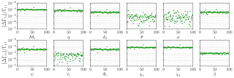
Figure 4: Relative difference of the Fisher matrices diagonal elements computed on a sample of 100 events with GWFAST and an independent Wolfram Mathematica code. The labels of the $x$–axes refer to the parameters whose diagonal elements are plotted.

4 Covariance matrix

In the limit of linear signal (or large SNR) and in presence of Gaussian noise the inverse of the FIM gives the covariance of the Bayesian posterior probability distribution of the true waveform parameters for a given experiment, assuming a flat prior. The inversion of the matrix can become problematic if the condition number (i.e. the ratio of absolute values of the largest to smallest eigenvalues) is larger than the inverse machine precision. This is the case for highly correlated or nearly degenerate combinations of parameters. In this case, the linear signal approximation might break down in some regions of the likelihood surface (Vallisneri, 2008).

4.1 Fisher matrix inversion

Tools for obtaining the covariance and analyzing the reliability of the inversion are contained in the module fisherTools. Note that all the functions described here assume that the input FIM is an array of matrices in the last dimension, as described in Sect. 3.2 The conditioning of the FIM can be checked in GWFAST via the function CheckFisher, which returns the eigenvalues, eigenvectors, and condition number of the matrix. The inversion of the FIM to yield the covariance is done with the function CovMatr, as

⬇

import fisherTools as fTools

CovMatrsNet, inversion_errors = fTools.CovMatr(FisherMatrsNet)

Code example 11: Computation of covariance matrices from Fisher matrices in GWFAST.

By default, each row and column is normalized to the square root of the diagonal of the FIM before inversion, so that the resulting matrix has adimensional entries with ones on the diagonal and the remaining elements in the interval $[-1,\,1]$ (Harms et al., 2022). The inverse transformation is applied after inversion to yield the inverse of the original matrix. GWFAST also implements a variety of possibilities for the technique used to find the inverse. The Python library for precision arithmetic mpmath is used for the inversion. The inversion is not performed if the condition number is larger than a threshold that can be specified by the user via the argument condNumbMax. Its default value is $10^{50}$ (so the code will try to invert every matrix irrespective of the conditioning). The available possibilities are listed below, and can be specified by the argument invMethodIn:

'inv'

inverse computed by mpmath;

'cho'

inverse computed by means of the Cholesky decomposition, i.e. the (Hermitian, positive–definite) FIM is expressed as a product of a lower triangular matrix and its conjugate transpose, and the latter is inverted. This is the default option in GWFAST;

'svd'

the singular–value decomposition (SVD) of the FIM is used to invert the matrix. In this case, there is the additional option of truncating the smallest singular values to the minimum allowed numerical precision, that can help regularizing badly conditioned matrices. This can be required by setting the Boolean truncate=True. In this case, for each singular value $s$, if the ratio of its absolute value to the absolute value of the largest singular value, $\max{s_{i}}$, is smaller than a threshold $\lambda$, the singular value $s$ is replaced with $\lambda\times\max{(s_{i})}$. The value of the threshold $\lambda$ can be specified with the argument svals_thresh which is set by default to $10^{15}$;

'svd_reg'

the singular–value decomposition (SVD) of the FIM is used to invert the matrix, and eigenvalues smaller than the threshold specified by the argument svals_thresh are not included in the inversion. This ensures that the error on badly constrained parameters is not propagated to the other ones (Harms et al., 2022). However, it might result in underestimating the uncertainty for parameters whose eigenvalues are excluded, and the effect should be carefully checked.

'lu'

inversion is done by means of the Lower–Upper (LU) decomposition, i.e. the factorization of the FIM into the product of one lower triangular matrix and one upper triangular matrix. This can be a useful option since, as for the Cholesky decomposition, the inversion of a triangular matrix is easier than the one of a full matrix. Differently from the Cholesky decomposition, however, the original matrix does not have to be hermitian and positive–definite, which can make this method more stable against numerical noise for badly–conditioned matrices.

The error on the inversion is computed in GWFAST by the function compute_inversion_error with the definition $\epsilon={||\Gamma\cdot\Gamma^{-1}-\mathbb{1}||}_{\rm max}={\rm max}_{ij}|(\Gamma\cdot\Gamma^{-1}-\mathbb{1})_{ij}|$, where $\mathbb{1}$ denotes the identity matrix, $\Gamma$ the FIM and $\Gamma^{-1}$ its inverse as computed by the code

⬇

invErrs = fTools.compute_inversion_error(FisherMatrsNet, CovMatrsNet)

Code example 12: Computation of the inversion errors in GWFAST.

Two other utilities to check the quality of the inversion are available in GWFAST in the module fisherTools. The function check_covariance computes the inversion error, and prints the difference between $\Gamma\cdot\Gamma^{-1}$ and the identity on the diagonal, and the off–diagonal elements of $\Gamma\cdot\Gamma^{-1}$ exceeding a given threshold specified with the argument tol. Secondly, the function perturb_Fisher adds random perturbations to the FIM to a specified decimal (given by the argument eps, whose default is ${10}^{-10}$), and checks if the inversion remains stable.

While the squared root of the diagonal elements of the covariance matrix give the expected marginalized $1\sigma$ errors on the parameters, a useful metric for GW parameter estimation is the sky localization region at some given confidence level. This is computed by (Barack & Cutler, 2004; Wen & Chen, 2010)

$$\Delta\Omega_{{\rm X}\%}=-2\pi|\sin\theta|\mathchoice{{\hbox{$\displaystyle\sqrt{\left(\Gamma^{-1}\right)_{\theta\theta}\,\left(\Gamma^{-1}\right)_{\phi\phi}-\left(\Gamma^{-1}\right)_{\theta\phi}^{2}\,}$}\lower 0.4pt\hbox{\vrule height=9.30444pt,depth=-7.44359pt}}}{{\hbox{$\textstyle\sqrt{\left(\Gamma^{-1}\right)_{\theta\theta}\,\left(\Gamma^{-1}\right)_{\phi\phi}-\left(\Gamma^{-1}\right)_{\theta\phi}^{2}\,}$}\lower 0.4pt\hbox{\vrule height=9.30444pt,depth=-7.44359pt}}}{{\hbox{$\scriptstyle\sqrt{\left(\Gamma^{-1}\right)_{\theta\theta}\,\left(\Gamma^{-1}\right)_{\phi\phi}-\left(\Gamma^{-1}\right)_{\theta\phi}^{2}\,}$}\lower 0.4pt\hbox{\vrule height=6.53888pt,depth=-5.23112pt}}}{{\hbox{$\scriptscriptstyle\sqrt{\left(\Gamma^{-1}\right)_{\theta\theta}\,\left(\Gamma^{-1}\right)_{\phi\phi}-\left(\Gamma^{-1}\right)_{\theta\phi}^{2}\,}$}\lower 0.4pt\hbox{\vrule height=5.03888pt,depth=-4.03113pt}}}\ \ln{\left(1-{{\rm X}}/{100}\right)}\,.$$ (6)

The function compute_localization_region computes the sky localization region, in square degrees or steradian, according to the previous definition. The desired units can be specified through the units key, which can have values 'SqDeg' and 'Sterad', and the confidence level is specified by the optional argument perc_level (the default $90\%$). An example of usage is presented in 13.

4.2 Manipulating the Fisher and covariance matrices

The Fisher approach allows to treat straightforwardly some common situations encountered in parameter estimation, which we summarize here together with a description of their implementation in GWFAST. All functions described in the following belong to the module fisherTools:

• In order to fix some parameters to their fiducial values, one has to remove from the FIM (before inverting it) the corresponding rows and columns. This is done with the function fixParams, which takes the following arguments (in the order they are listed here): the original matrix, the dictionary specifying the position of each parameter in the FIM (accessible from the waveform object, see the end of Sect. 2.2 for an explanation), and a list of string with names of the parameters to be fixed, with the same names as in Tab. 1. The function returns the new matrix, and a dictionary of the same form of the input dictionary, with the keys corresponding to the fixed parameters removed, and the remaining rescaled;

• In order to add a Gaussian prior on some parameters, one has to add to the FIM a prior matrix $P_{ij}$ corresponding to the inverse covariance of the prior. For the moment, GWFAST supports the addition of a diagonal prior matrix. This can be done with the function addPrior, which takes as input the original matrix, a list of values to be added on the diagonal of the Fisher (representing thus the inverse covariance of the prior on the corresponding parameter), the dictionary specifying the position of each parameter in the FIM, and the list of names of parameters on which the prior should be added;

• In order to marginalize over some parameters, one has to remove from the covariance matrix (after the inversion of the FIM) the corresponding rows and columns. This can be done again with the function fixParams described in the first point.

⬇

# Fix spins to their fiducial values

FisherMatrsNet_fix_spins, pars_nospin = fTools.fixParams(FisherMatrsNet, pars, ['chi1z', 'chi2z'])

# Add Gaussian prior on theta, phi, iota, psi, phicoal

angles = ['theta', 'phi', 'iota', 'psi', 'Phicoal']

priors_vals = np.repeat(1/(2*np.pi**2), len(angles))

FisherMatrsNet_fix_spins_prior = fTools.addPrior(FisherMatrsNet_fix_spins, priors_vals, pars_nospin, angles)

# Invert the new FIM

CovMatrsNet_fix_spins_prior, inversion_errors_fix_spins_prior = fTools.CovMatr( FisherMatrsNet_fix_spins_prior)

# Compute 90% localization area in square degrees

sky_loc = fTools.compute_localization_region(CovMatrsNet_fix_spins_prior, pars_nospin, events['theta'], perc_level=90, units='SqDeg')

Code example 13: Example of manipulations of the Fisher matrix: fix the spins to their fiducial values, add a Gaussian prior on the angles with standard deviation $2\pi$, compute the corresponding covariance, compute the forecasted $90\%$ localization region in square degrees.

5 Running in parallel

Besides the accuracy in the computation of the derivatives, the main advantage of the use of JAX (Bradbury et al., 2018) is that it allows us to vectorize the calculation of the FIM. The typical usage of a code as GWFAST consists in forecasting parameter estimation capabilities for large catalogs of sources, which is clearly a parallel problem. JAX and GWFAST allow us to vectorize the calculation even on a single CPU, which can be used in combination with parallelization routines. GWFAST includes the executable calculate_forecasts_from_catalog.py that implements such parallelization and is ready to use both on single machines and on clusters.

A catalog has to be stored in .h5 format in the folder data/. A function to save a catalog of the form given in 1 is included in the module gwfastUtils:

⬇

from gwfastUtils import save_data

# save events in .h5 format

save_data('file_name.h5', events)

Code example 14: How to save an event catalog in GWFAST.

calculate_forecasts_from_catalog.py divides the events in the catalog into batches of size specified by the user with the option --batch_size, and splits the calculations assigning a given number of batches to each parallel process. The number of processes is controlled by the option --npools. Events in a single batch are computed in vectorized form for each process, which results effectively in a gain of speed of a factor that can be at most equal to the batch size with respect to a non–vectorized implementation. calculate_forecasts_from_catalog.py allows both the use of multiprocessing (McKerns et al., 2012) on a single machine and the use of MPI (Dalcin & Fang, 2021) on clusters. The usage is as follows:

⬇

> mkdir my_results

> python calculate_forecasts_from_catalog.py --fout=my_results --fname_obs FNAME_OBS [--wf_model WF_MODEL] [--batch_size BATCH_SIZE]

[--npools NPOOLS] [--snr_th SNR_TH] [--idx_in IDX_IN] [--idx_f IDX_F] [--fmin FMIN]

[--fmax FMAX] [--compute_fisher COMPUTE_FISHER] [--net NET [NET ...]] [--rot ROT]

[--netfile NETFILE] [--psds PSDS [PSDS ...]] [--mpi MPI] [--duty_factor DUTY_FACTOR]

[--params_fix PARAMS_FIX [PARAMS_FIX ...]] [--lalargs LALARGS [LALARGS ...]]

[--return_all RETURN_ALL] [--seeds SEEDS [SEEDS ...]]

Code example 15: How to run GWFAST on a catalog of events through the script calculate_forecasts_from_catalog.py.

The options are as follows:

fout

string; path to output folder, which has to exist before the script is launched;

fname_obs

string; name of the file containing the catalog without the extension .h5;

wf_model

string; name of the waveform model, default is 'tf2'. Options are: 'tf2', 'tf2_tidal', 'tf2_ecc', 'IMRPhenomD', 'IMRPhenomD_NRTidalv2', 'IMRPhenomHM', 'IMRPhenomNSBH'. It is also possible to choose all the other waveform models available in LAL, by passing 'LAL-wfname', where wfname is the name of the chosen waveform in LAL, e.g. 'LAL-IMRPhenomXPHM';

batch_size

int, default is 1; size of the batch to be computed in vectorized form on each process;

npools

int, default is 1; number of parallel processes;

snr_th

float, default is 12.; threshold value for the SNR to consider the event detectable. FIMs are computed only for events with SNR exceeding this value;

idx_in

int, default is 0; index of the event in the catalog from which to start the calculation;

idx_f

int, default is -1 (meaning all events); index of the event in the catalog from which to end the calculation;

fmin

float, default is 2.; minimum frequency of the grid in $\text{\,}\mathrm{H}\mathrm{z}$;

fmax

float, default is None; maximum frequency in $\text{\,}\mathrm{H}\mathrm{z}$. If not specified, coincides with the cut frequency of the waveform;

compute_fisher

int, default is 1; if 0, only SNRs are computed, if 1 the code also computes FIMs;

net

list of string, default is ['ETS']; the network of detectors chosen. Pre–defined configurations are passed using the names in Tab. 2 separated by single spacing. Other configurations can be added directly to the dictionary detectors in the module gwfastGlobals. Alternatively, one can pass a custom configuration with the option netfile;

psds

list of string, default is ['ET-0000A-18.txt']; the paths to PSDs of each detector in the network inside the folder psds/, separated by single spacing;

netfile

alternative to the use of net and psds to configure the detector network; a dictionary containing the configuration can be saved in .json format and passed as input. It is possible to save a network configuration as:

⬇

from gwfastUtils import save_detectors

my_network = {'my_detector_1': { 'lat': ..., 'long': ... , 'xax': ... ,

'shape': ... , 'psd_path': 'path/to/psd'},

'my_detector_2': {...}

}

save_detectors('network_file_name.json', my_network)

Code example 16: How to save a detector network configuration for GWFAST.

then, send run with --netfile=network_file_name.json;

mpi

int, default is 1; if 0, the code parallelizes using multiprocessing, if 1, it parallelizes using MPI, suitable for clusters. In this case, the function should be called accordingly, e.g.

⬇

> mpirun -n 4 python calculate_forecasts_from_catalog.py ... --mpi=1 --npools=4

Code example 17: How to parallelize a run using MPI.

duty_factor

float $\in[0,1]$, default is 1.; duty factor of the detectors. This is applied separately to each detector in the network (and to each component separately in the case of a triangular configuration);

params_fix

list of string, default is [ ]; parameters to fix to the fiducial values, i.e. to eliminate from the FIM;

rot

int, default is 1; if 0 the effect of the rotation of the Earth is not included in the analysis, if 1 it is included;

lalargs

list of string, default is [ ]; specifications of the waveform when using LAL interface. This has to contain 'HM' if the waveform includes the contribution of higher–order modes, 'tidal' if it contains tidal effects, 'precessing' if it includes precessing spins, and 'eccentric' if it includes eccentricity;

return_all

int, default is 1; if 1, in case a network of detectors is used, the SNRs and Fishher matrices of the individual detector are also stored;

seeds

list of int, default is [ ]; list of seeds to set for the duty factors in individual detectors, to make the results easily reproducible.

To show the performance gain using vectorization, we report in Fig. 5 the ratio $t/(Nt_{1})$ among the time $t$ needed to compute SNRs and Fisher matrices on $N$ events at the same time on the same CPU, and $N$ times the time $t_{1}$ needed to compute the same quantities for 1 event (which is the time needed using a for loop). From the left panel, referring to the SNRs, the impressive gain brought by vectorization is apparent, with an amount of time need for the computation that stays basically constant while enlarging the batch size, thus effectively being $N$ times faster than a loop–based computation. Quantifying the advantage from vectorization when computing Fisher matrices is instead more subtle: as it is apparent from the right panel of Fig. 5, for $N\gtrsim 10$ the behaviour has a dependence on the characteristics of the machine used to run the code. Differently from SNRs, Fisher matrices need much more memory to be allocated during the computation, especially when vectorizing on $N$ events, and the operations can become much slower on these large arrays, eventually leading to a loss in terms of speed as compared to a serial computation, which instead handles smaller arrays. In any case, there is always an ‘optimal’ batch size, depending on the machine’s characteristics, such that the gain in terms of speed thanks to vectorization can be as large as a factor of $\sim 5$.

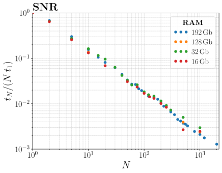
(a)

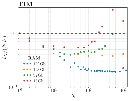
(b)

Figure 5: Ratio of the time needed to compute SNRs (left) and Fisher matrices (right) vectorizing on $N$ events, and the time needed to perform the computation serially, with a for loop (equivalent to $N$ times the time needed for a single evaluation). The different colors refer to the results obtained using machines with different characteristics, as reported in the legend.

6 Comparison with real events

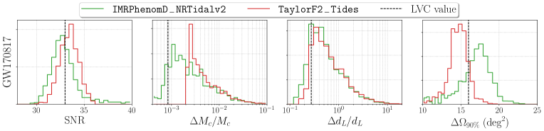
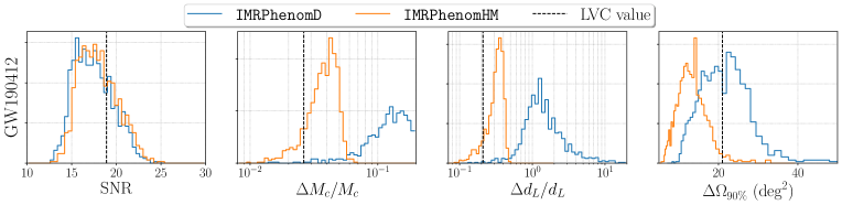
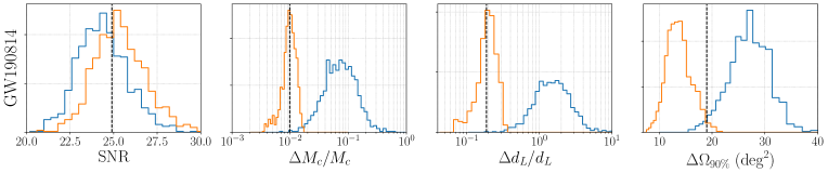
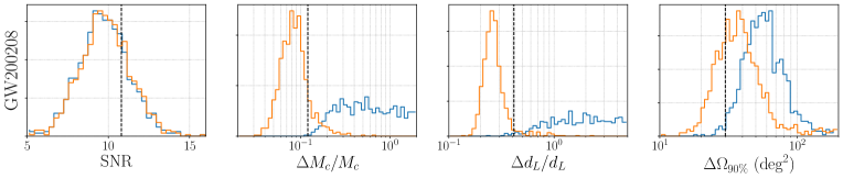
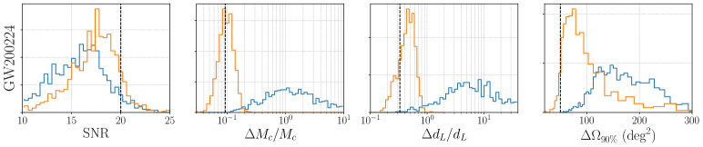
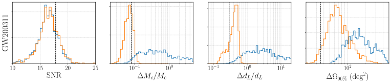
Figure 6: Comparison of the results obtained using GWFAST for some selected events from GWTC–2 and GWTC–3: GW170817, GW190412, GW190814, GW200208_130117, GW200224_222234 and GW200311_115853. Each row contains the histogram of the SNR, $90\%$ relative credible intervals on the source–frame chirp mass and luminosity distance, and 90%–credible sky area for 1000 samples of the posterior distributions of the events for all the parameters. Lines of different colours refer to different waveform models and the vertical dashed lines denote the errors inferred by LVC with a full Bayesian parameter estimation (Abbott et al., 2021b, a).

As an illustration of the reliability of GWFAST, we checked how its predictions compare to the SNRs and measurement errors associated to real events. This is a stringent test since, for currently available events, many assumptions on which the FIM approximation is based are of course not valid, in particular the Gaussianity of the noise and the limit of high SNR. Here we show that we can still reproduce correctly the order of magnitude of SNRs and relative errors, taking into account the broad measurement errors of the real events. We selected a subset of the GW events in GWTC–1, GWTC–2 and GWTC–3, with ${\rm SNR}\geq 10$ and sky localization $\Delta\Omega_{90\%}\leq$50\text{\,}{\mathrm{deg}}^{2}$$. For each selected event we extracted 1000 samples from the full set of posterior samples for each parameter. We used ASDs obtained averaging the strain of each detector in a window of 1024 seconds around each event,¹⁹ using Welch’s method, through the software GWpy (Macleod et al., 2021).

The results for GW170817 (BNS), GW190412, GW190814, GW200208_130117, GW200224_222234 and GW200311_115853 (BBHs) are shown in Fig. 6, where we compare the errors estimated from GWFAST on the set of 1000 samples drew for each event to the actual measurement errors obtained from the full Bayesian analysis (which can be read from Tab. III of Abbott et al. (2019) for the events belonging to GWTC–1, Tab. VI of Abbott et al. (2021b) for those belonging to GWTC–2, and Tab. IV of Abbott et al. (2021a) for those belonging to GWTC–3). In particular, we show the distribution of the SNRs, the 90% relative credible intervals on the source–frame chirp mass, $M_{c}$, and luminosity distance and the size of the 90%–credible sky area, and report as a dashed line the LVK error estimate. For the BNS event GW170817 we performed the analysis with the waveform models TaylorF2_Tides and IMRPhenomD_NRTidalv2, both including tidal effects, while for the BBH events we used IMRPhenomD and IMRPhenomHM, which includes the contribution of higher modes, always taken into account in the parameter estimation of the chosen BBH signals (Abbott et al., 2020b, c, 2021a).

We find overall a very good agreement for the SNR distributions for all events, with both the waveform models used in each case, and we also observe that, as expected in the BBH case, IMRPhenomHM produces slightly higher SNRs than IMRPhenomD, especially for GW190814. This can be traced to the fact that the mass ratio of this system is large (the primary component has been estimated to have a source–frame mass of about $23\text{\,}\mathrm{M_{\odot}}$ and the secondary $2.6\text{\,}\mathrm{M_{\odot}}$), resulting in a greater relevance of the sub–dominant modes, as compared to more symmetric binaries (see e.g. Fig. 2 of Puecher et al. (2022)).

Regarding GW170817, we find that the agreement of the fractional error on the chirp mass $M_{c}$ with the LVK estimate, despite the long inspiral, is better using the full inspiral–merger–ringdown model IMRPhenomD_NRTidalv2, which was not included in the first analysis of the system, while the distributions of the fractional error on $d_{L}$ are similar, and the distribution of the sky localization $\Delta\Omega_{90\%}$ are compatible.

For the majority of the BBH systems, we find our estimations on the source–frame chirp mass and luminosity distance errors to be compatible with the values inferred by LVK when using the waveform model including higher–order harmonics, which were indeed included in the analysis. The only exception is the system GW200208_130117, for which our estimations seem optimistic. This can be understood by the fact that the network SNR for this system (equal to 10.8) is the lowest among the ones considered: for such a value of the SNR, the FIM approach is not guaranteed to work. In any case, even in this case the sky localization is compatible and there is always a fraction of cases where also the fractional errors on chirp mass and distance are consistent. As for the sky localisation, we find our estimations to include the LVK results for all the events when using IMRPhenomHM, always being on the same order of magnitude and without a clear trend towards higher or lower values for different events.

7 Summary

In this article we presented GWFAST , a novel pure Python code for computing SNRs and Fisher information matrices for catalogs of GW events, in a fast, accurate and user–friendly way. In particular, GWFAST:

• implements a pure Python version of state–of–the–art Fourier domain full inspiral–merger–ringdown waveform models, suitable for both BBH, BNS and NSBH systems, namely IMRPhenomD, IMRPhenomD_NRTidalv2, IMRPhenomHM and IMRPhenomNSBH. These are also separately available in the module WF4Py  (which further includes the waveform model IMRPhenomXAS), and allow to exploit vectorization to speed up the computation and to employ automatic differentiation for computing derivatives. It is also possible to use all waveforms included in LAL, in which case derivatives are computed with finite differences techniques;

• accounts for the amplitude and phase modulation of the observed GW signal due to Earth’s rotation, which is of fundamental importance at 3G detectors, whose sensitivity curve can extend down to $2\text{\,}\mathrm{Hz}$, in particular for BNS systems, which can stay in the detection band for as long as $\order{$1\text{\,}\mathrm{day}$}$;

• is developed to handle networks of detectors, both L–shaped and triangular, and includes 10 pre–defined locations as well as several sensitivity curves, for both current and planned ground–based detectors, which can also easily be extended;

• if waveforms in Python are used, computes derivatives using automatic differentiation, through the JAX package, thus being extremely accurate and fast, and offers the possibility of computing derivatives with respect to many parameters analytically, to further speed up the computation;

• handles the inversion of the FIM using the mpmath library, thus avoiding limitations linked to numerical precision, and includes functions for easily manipulating both the Fisher and covariance matrices, e.g. adding priors or computing localisation regions, as well as tools to assess the reliability of the inversion;

• can compute SNRs and Fisher matrices for multiple events at a time on a single CPU exploiting Python vectorization, and provides a module for parallelization over multiple CPUs, also suitable for clusters, thus being ideal for large catalogs of sources;

We assessed the reliability of GWFAST in computing accurately the signal derivatives, as well as the frequency integral, by comparing with an independent code written in Wolfram Mathematica, capable of computing analytical derivatives with respect to all parameters, obtaining excellent agreement. We further compared the predictions for the SNRs and measurement errors obtained using GWFAST on some of the loudest and best localised events detected during the second and third observing runs of the LVK collaboration with the actual results obtained from a full Bayesian parameter estimation, obtaining good agreement. GWFAST has been used to produce the results in the companion paper (Iacovelli et al., 2022), where we also discuss its comparison with other existing codes and results (Borhanian, 2021; Pieroni et al., 2022; Harms et al., 2022), showing their excellent agreement. Due to its structure and to the use of automatic differentiation, GWFAST is also suitable for extensions of the FIM approximation (Sellentin et al., 2014; Vallisneri, 2011; Wang et al., 2022). We are confident that it will constitute a useful tool for assessing the scientific potential of third–generation GW detectors. GWFAST is publicly available at https://github.com/CosmoStatGW/gwfast. This paper is associated to version v1.0.1 which is archived on Zenodo (Iacovelli & Mancarella, 2022). The library WF4Py is available at https://github.com/CosmoStatGW/WF4Py. This paper is associated to version v1.0.0 which is archived on Zenodo (Iacovelli, 2022).

References

- Abbott et al. (2019) Abbott, B., et al. 2019, Phys. Rev. X, 9, 031040, doi: 10.1103/PhysRevX.9.031040
- Abbott et al. (2017) Abbott, B. P., et al. 2017, Class. Quant. Grav., 34, 044001, doi: 10.1088/1361-6382/aa51f4
- Abbott et al. (2020a) —. 2020a, Living Rev. Rel., 23, 3, doi: 10.1007/s41114-020-00026-9
- Abbott et al. (2020b) Abbott, R., et al. 2020b, Phys. Rev. D, 102, 043015, doi: 10.1103/PhysRevD.102.043015
- Abbott et al. (2020c) —. 2020c, Astrophys. J., 896, L44, doi: 10.3847/2041-8213/ab960f
- Abbott et al. (2021a) —. 2021a. https://arxiv.org/abs/2111.03606
- Abbott et al. (2021b) —. 2021b, Phys. Rev. X, 11, 021053, doi: 10.1103/PhysRevX.11.021053
- Ajith (2011) Ajith, P. 2011, Phys. Rev. D, 84, 084037, doi: 10.1103/PhysRevD.84.084037
- Barack & Cutler (2004) Barack, L., & Cutler, C. 2004, Phys. Rev. D, 69, 082005, doi: 10.1103/PhysRevD.69.082005
- Borhanian (2021) Borhanian, S. 2021, Class. Quant. Grav., 38, 175014, doi: 10.1088/1361-6382/ac1618
- Bradbury et al. (2018) Bradbury, J., Frostig, R., Hawkins, P., et al. 2018, JAX: composable transformations of Python+NumPy programs, 0.2.5. http://github.com/google/jax
- Buonanno et al. (2009) Buonanno, A., Iyer, B., Ochsner, E., Pan, Y., & Sathyaprakash, B. S. 2009, Phys. Rev. D, 80, 084043, doi: 10.1103/PhysRevD.80.084043
- Cutler & Flanagan (1994) Cutler, C., & Flanagan, E. E. 1994, Phys. Rev. D, 49, 2658, doi: 10.1103/PhysRevD.49.2658
- Dalcin & Fang (2021) Dalcin, L., & Fang, Y.-L. L. 2021, Computing in Science & Engineering, 23, 47, doi: 10.1109/MCSE.2021.3083216
- Dietrich et al. (2019) Dietrich, T., Samajdar, A., Khan, S., et al. 2019, Phys. Rev. D, 100, 044003, doi: 10.1103/PhysRevD.100.044003
- Freise et al. (2009) Freise, A., Chelkowski, S., Hild, S., et al. 2009, Classical and Quantum Gravity, 26, 085012, doi: 10.1088/0264-9381/26/8/085012
- Gossan et al. (2022) Gossan, S. E., Hall, E. D., & Nissanke, S. M. 2022, Astrophys. J., 926, 231, doi: 10.3847/1538-4357/ac4164
- Harms et al. (2022) Harms, J., Dupletsa, U., Banerjee, B., et al. 2022. https://arxiv.org/abs/2205.02499
- Husa et al. (2016) Husa, S., Khan, S., Hannam, M., et al. 2016, Phys. Rev. D, 93, 044006, doi: 10.1103/PhysRevD.93.044006
- Iacovelli (2022) Iacovelli, F. 2022, WF4Py: Gravitational waves waveform models in pure Python language, v1.0.0, Zenodo, doi: 10.5281/zenodo.7060240
- Iacovelli & Mancarella (2022) Iacovelli, F., & Mancarella, M. 2022, gwfast: a Fisher information matrix Python package for GW detector networks, v1.0.1, Zenodo, doi: 10.5281/zenodo.7060236
- Iacovelli et al. (2022) Iacovelli, F., Mancarella, M., Foffa, S., & Maggiore, M. 2022. https://arxiv.org/abs/2207.02771
- Kalaghatgi et al. (2020) Kalaghatgi, C., Hannam, M., & Raymond, V. 2020, Phys. Rev. D, 101, 103004, doi: 10.1103/PhysRevD.101.103004
- Khan et al. (2016) Khan, S., Husa, S., Hannam, M., et al. 2016, Phys. Rev. D, 93, 044007, doi: 10.1103/PhysRevD.93.044007
- LIGO Scientific Collaboration (2018) LIGO Scientific Collaboration. 2018, LIGO Algorithm Library - LALSuite, free software (GPL), doi: 10.7935/GT1W-FZ16
- London et al. (2018) London, L., Khan, S., Fauchon-Jones, E., et al. 2018, Phys. Rev. Lett., 120, 161102, doi: 10.1103/PhysRevLett.120.161102
- Macleod et al. (2021) Macleod, D. M., Areeda, J. S., Coughlin, S. B., Massinger, T. J., & Urban, A. L. 2021, SoftwareX, 13, 100657, doi: 10.1016/j.softx.2021.100657
- Maggiore (2007) Maggiore, M. 2007, Gravitational Waves. Vol. 1: Theory and Experiments, Oxford Master Series in Physics (Oxford University Press)
- Margossian (2018) Margossian, C. C. 2018, CoRR, abs/1811.05031
- McKerns et al. (2012) McKerns, M. M., Strand, L., Sullivan, T., Fang, A., & Aivazis, M. A. G. 2012, arXiv e-prints, arXiv:1202.1056. https://arxiv.org/abs/1202.1056
- Mishra et al. (2016) Mishra, C. K., Kela, A., Arun, K. G., & Faye, G. 2016, Phys. Rev. D, 93, 084054, doi: 10.1103/PhysRevD.93.084054
- Moore et al. (2016) Moore, B., Favata, M., Arun, K. G., & Mishra, C. K. 2016, Phys. Rev. D, 93, 124061, doi: 10.1103/PhysRevD.93.124061
- Pannarale et al. (2015) Pannarale, F., Berti, E., Kyutoku, K., Lackey, B. D., & Shibata, M. 2015, Phys. Rev. D, 92, 084050, doi: 10.1103/PhysRevD.92.084050
- Pieroni et al. (2022) Pieroni, M., Ricciardone, A., & Barausse, E. 2022. https://arxiv.org/abs/2203.12586
- Pratten et al. (2020) Pratten, G., Husa, S., Garcia-Quiros, C., et al. 2020, Phys. Rev. D, 102, 064001, doi: 10.1103/PhysRevD.102.064001
- Puecher et al. (2022) Puecher, A., Kalaghatgi, C., Roy, S., et al. 2022. https://arxiv.org/abs/2205.09062
- Rodriguez et al. (2013) Rodriguez, C. L., Farr, B., Farr, W. M., & Mandel, I. 2013, Phys. Rev. D, 88, 084013, doi: 10.1103/PhysRevD.88.084013
- Schutz (2011) Schutz, B. F. 2011, Class. Quant. Grav., 28, 125023, doi: 10.1088/0264-9381/28/12/125023
- Sellentin et al. (2014) Sellentin, E., Quartin, M., & Amendola, L. 2014, Mon. Not. Roy. Astron. Soc., 441, 1831, doi: 10.1093/mnras/stu689
- Smith et al. (2021) Smith, R., et al. 2021, Phys. Rev. Lett., 127, 081102, doi: 10.1103/PhysRevLett.127.081102
- Srivastava et al. (2022) Srivastava, V., Davis, D., Kuns, K., et al. 2022, Astrophys. J., 931, 22, doi: 10.3847/1538-4357/ac5f04
- Vallisneri (2008) Vallisneri, M. 2008, Phys. Rev. D, 77, 042001, doi: 10.1103/PhysRevD.77.042001
- Vallisneri (2011) —. 2011, Phys. Rev. Lett., 107, 191104, doi: 10.1103/PhysRevLett.107.191104
- Wade et al. (2014) Wade, L., Creighton, J. D. E., Ochsner, E., et al. 2014, Phys. Rev. D, 89, 103012, doi: 10.1103/PhysRevD.89.103012
- Wang et al. (2022) Wang, Z., Liu, C., Zhao, J., & Shao, L. 2022, Extending the Fisher Information Matrix in Gravitational-wave Data Analysis. https://arxiv.org/abs/2203.02670
- Wen & Chen (2010) Wen, L., & Chen, Y. 2010, Phys. Rev. D, 81, 082001, doi: 10.1103/PhysRevD.81.082001