Higher-dimensional counterexamples to Hamiltonicity

Abstract

For $d\geq 2$, we show that all graphs of $d$-polytopes have Hamiltonian line graph if and only if $d\neq 3$: We exhibit a graph of a $3$-polytope on $252$ vertices whose line graph is not even traceable. Adapting a construction by Grünbaum and Motzkin, for large $n$ we also construct simple 3-polytopes on $3n$ vertices in whose line graph any simple path is shorter than $10n^{\alpha}$, for some constant $\alpha<1$. Moreover, we give four elementary counterexamples of plausible extensions to simplicial complexes of four famous results in Hamiltonian graph theory, namely:

1. There is a $2$-complex without (tight, loose, or weak) Hamiltonian paths, where every vertex is in more than $\frac{n}{2}$ facets.

2. There is a $2$-complex without (tight, loose, or weak) Hamiltonian paths that is maximally non-weakly-Hamiltonian.

3. There is a $2$-complex without (tight, loose, or weak) Hamiltonian paths that is self-complementary.

4. There is a 2-strongly connected 2-complex whose square complex has no (tight, loose, or weak) Hamiltonian cycles.

Introduction

Hamiltonian graphs are named after sir William Rowan Hamilton, who in 1857 invented a commercial puzzle of finding a cycle on the edges of a dodecahedron, with the condition that every vertex should be visited exactly once. Graphs with a path that visits all vertices once are instead called traceable. In 1880 Tait conjectured that all graphs of simple $3$-polytopes are Hamiltonian [33]; this was disproved 66 years later by Tutte’s graph [34]. In 1962 Grünbaum–Motzkin [18] and Moon–Moser [28] constructed $3$-polytopes whose graph is ‘far from being traceable’. By coning over such examples, they obtained $d$-polytopes with non-Hamiltonian graph for every $d\geq 4$. Barnette’s 1970 conjecture that “for $d\geq 4$, all graphs of simple $d$-polytopes are Hamiltonian” is still open.

In the first section of the paper, we focus on line–Hamiltonian graphs, i.e. graphs whose line graph is Hamiltonian. It is easy to see that all Eulerian and all Hamiltonian graphs are line-Hamiltonian [10]. The converse is false: For example, Tutte’s graph mentioned above is line-Hamiltonian, even if it is neither Eulerian nor Hamiltonian. We establish the following relation to polytopality:

Theorem I (Propositions 4, 5).

Let $d\geq 2$ be an integer. All graphs of $d$-polytopes are line-Hamiltonian if and only if $d\neq 3$. In fact, there is a $3$-polytope on $252$ vertices whose graph has a line graph that is not traceable. Moreover, for any $n$, there exists a simple 3-polytope on $3n$ vertices whose graph has a line graph in which every simple path is shorter than $10n^{\alpha}$, for some constant $\alpha<1$.

Thus $3$-polytopes can be ‘arbitrarily far’ from being line-traceable. See Proposition 11 for an extension to spheres, pseudomanifolds, or Gorenstein subspace arrangements. En passant, we prove in Proposition 8 that the dual graph of any polytopal pseudomanifold is $(d+1)$-connected, a fact that in the simplicial case had been proven long ago by Klee [25].

Through extensive computer search, we also tested a big portion of the non-Hamiltonian planar 3-regular graphs generated by Brinkmann and McKay [8]. All of them turned out to be line-Hamiltonian (Theorem 3).

In the second part of the paper, we turn to the goal of extending the theory of Hamiltonian graphs to simplicial complexes of higher dimensions. In 1952 Dirac [16] proved that any graph with $n\geq 3$ vertices is Hamiltonian if every vertex has at least $\frac{n}{2}$ neighbors. This was later strengthened by Pósa [30] and Chvátal [13], who characterized the degree sequences that force a graph to have Hamiltonian paths or cycles [13], and managed to show that all self-complementary graphs are traceable [13]. A crucial observation in Chvátal’s proof is that every “maximally non-Hamiltonian” graph admits a Hamiltonian path.

For $d$-dimensional simplicial complexes, three distinct notions of “tight-Hamiltonian paths”, “loose-Hamiltonian paths”, and “weakly–Hamiltonian paths” were introduced in [27, 23, 4]. “Tight-” implies “loose-” implies “weakly-Hamiltonian”, but all three notions boil down to ordinary Hamiltonicity for $d=1$, i.e., for graphs. With these notions, some Dirac-type theorems have been achieved in higher-dimensions, but only for complexes with huge number of vertices [19, 24, 31], or with large ridge degree [23], or for complexes that are already known to be traceable [4]. We show a few obstacles to extending Chvatal’s aforementioned observation, Dirac’s theorem, or the traceability of self-complementary graphs to higher dimensions:

Theorem II (Propositions 13, 14, 15, 18).

We construct:

• For each $d\geq 2$, a $d$-complex without (tight, loose, or weak) Hamiltonian paths that is maximally non-weakly-Hamiltonian;

• For each $d\geq 2$, a $d$-complex without (tight, loose, or weak) Hamiltonian paths in which any of the $n=2d+2$ vertices is in at least $\binom{2d}{d-1}>\frac{n}{2}$ facets.

• A self-complementary $2$-complex without (tight, loose, or weak) Hamiltonian paths.

• A 2-strongly connected 2-complex whose “square” has no (tight, loose, or weak) Hamiltonian cycle.

The last item is an obstacle to extending Fleischner’s theorem, which claims that the “square” of every $2$-connected graph $G$ is Hamiltonian [17]; see Section 2 for definitions.

1 Line-Hamiltonian and non-line-Hamiltonian polytopes

By $\Sigma^{d}_{n}$ we mean the $d$-skeleton of the $(n-1)$-simplex on the vertices $1,\ldots,n$. By $\,H_{i}$ we mean the $d$-face of $\Sigma^{d}_{n}$ with vertices $i,i+1,i+2,\ldots,i+d$, where the sum is taken modulo $n$.

Definition 1.

A graph $G$ is line-Hamiltonian if it satisfies any of the following equivalent conditions (see e.g. [20] for the equivalence of (ii) and (iii)):

1. Its edges can be labeled $1,2,\ldots,e$, such that for all $i\in\{1,\ldots,e\}$, the edges $i$ and $i+1$ intersect; here $e+1$ is identified with $1$.

2. Its line graph is Hamiltonian.

3. Each edge has at least one endpoint on some closed simple path $P$ inside the graph (possibly consisting of a single vertex).

Similarly, we call a graph line-traceable if its dual graph is traceable.

It is easy to see that all Eulerian and all Hamiltonian graphs are line-Hamiltonian [10]. The converse is false: the graph $H=12,23,24,34,35,45,56$ is neither Eulerian nor Hamiltonian, yet the line graph is both. Also, all line-Hamiltonian graphs are connected, though not necessarily $2$-(edge)-connected, as shown by any cycle with some pendants attached. Note that if we attach two-edge paths to a cycle, we obtain a non-line-Hamiltonian graph.

More interesting examples arise from polytope theory: In 1946 Tutte constructed the first example of a $3$-dimensional simple polytope whose graph is not Hamiltonian [34], thereby disproving a long-standing conjecture by Tait [33]. It turns out that Tutte’s graph, as well as many others alike, is line-Hamiltonian:

Proposition 2.

The following graphs of simple $3$-polytopes are line-Hamiltonian: Tutte’s graph, the Barnette–Bosák–Lederberg graph, the Faulkner–Younger graphs on 42 and 44 vertices, the Grinberg graphs on 42, 44, and 46 vertices, and the Thomassen graph on 94 vertices.

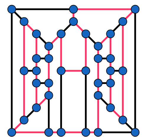
(a)

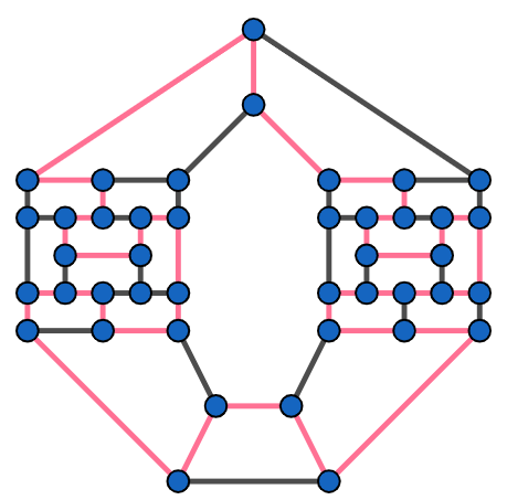
(b)

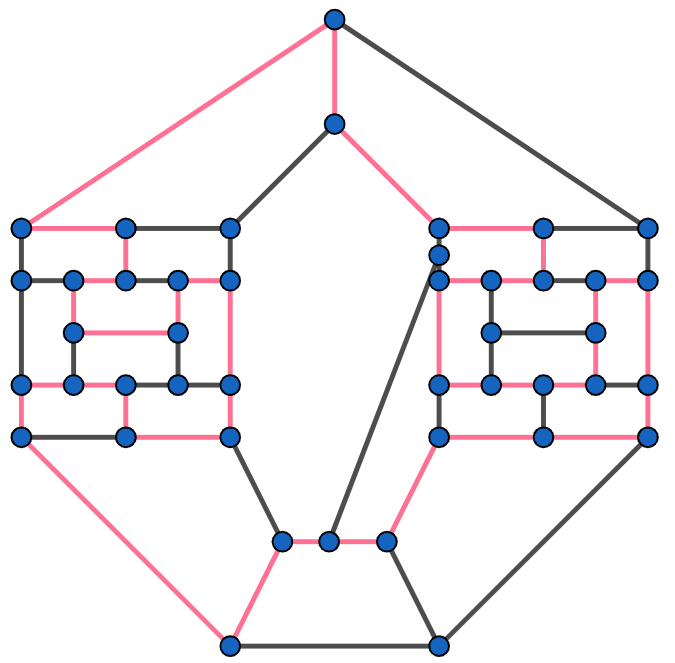
(c)

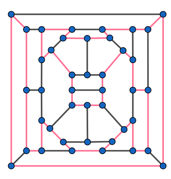
(d)

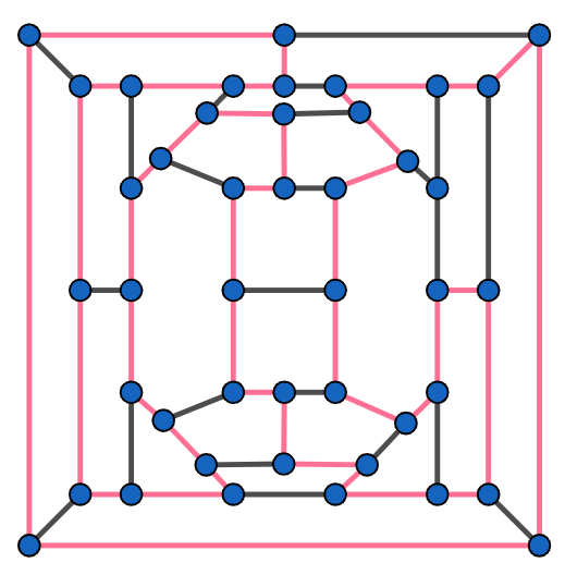
(e)

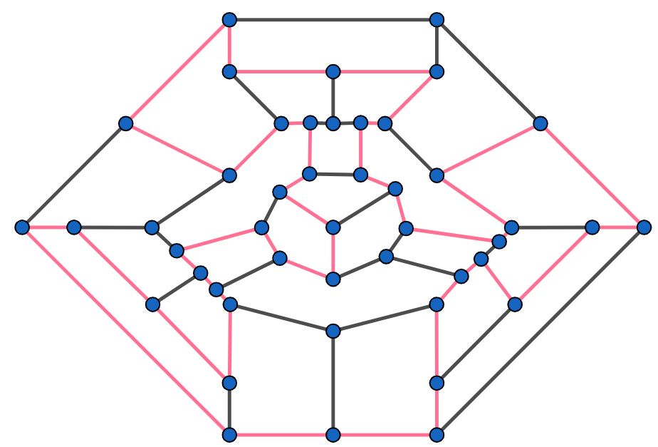
(f)

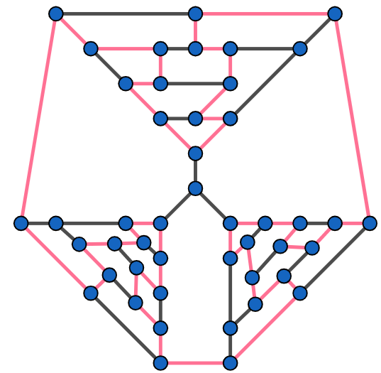
(g)

(h)

Figure 1.1: Closed paths proving the line-Hamiltonian property for: (a) the Bernette–Bosák–Ledergerg graph; (b),(c) the Faulkner–Younger graph on 42 resp. 44 vertices; (d), (e), (f) the Grinberg graph on 42, resp. 44, resp. 46 vertices; (g) Tutte’s graph; (h) the Thomassen graph on 94 vertices.

Proof by picture:.

For each of the listed non-Hamiltonian regular graphs, in Figure 1.1 we exhibit a closed simple path (in red) that via Definition 1, part (iii), proves the line-Hamiltonian property. ∎

Theorem 3.

All of the following planar 3-regular graphs are line-Hamiltonian:

• those with no faces of size 3 and with up to 48 vertices;

• those that are cyclically 4-connected with up to 50 vertices;

• those with no faces of size 3 or 4, with cyclic connectivity of exactly 4, and with up to 70 vertices;

• those that are cyclically 5-connected with up to 74 vertices.

Proof.

By extensive computer search on the non-Hamiltonian graphs generated by Brinkmann and McKay [8], we verified that all the graphs listed above are line-Hamiltonian. The class with no faces of size 3 or 4 and with cyclic connectivity of exactly 4 was the most challenging one for our server. Among these graphs with 70 vertices, roughly a dozen of them each required two weeks to be verified. Our script is run on a Quad Core CPU with the Neoverse N1 model, operating at a speed of 3.0 GHz. ∎

This seems to suggest that perhaps Tait’s question could be ‘updated’ by asking if regular polytopal graphs are line-Hamiltonian. For this follow-up question, the answer turns out to be negative for $d=3$, and positive otherwise:

Proposition 4.

Let $d\geq 2$ be an integer. The graphs of all $d$-polytopes are line-Hamiltonian if and only if $d\neq 3$. In fact, there is a simple $3$-polytope with $124$ vertices whose graph is line-traceable but not line-Hamiltonian, and a simple $3$-polytope on $252$ vertices whose graph is not line-traceable.

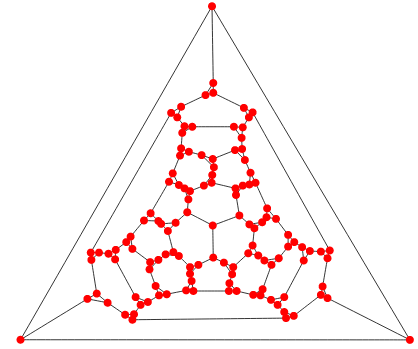
(a)

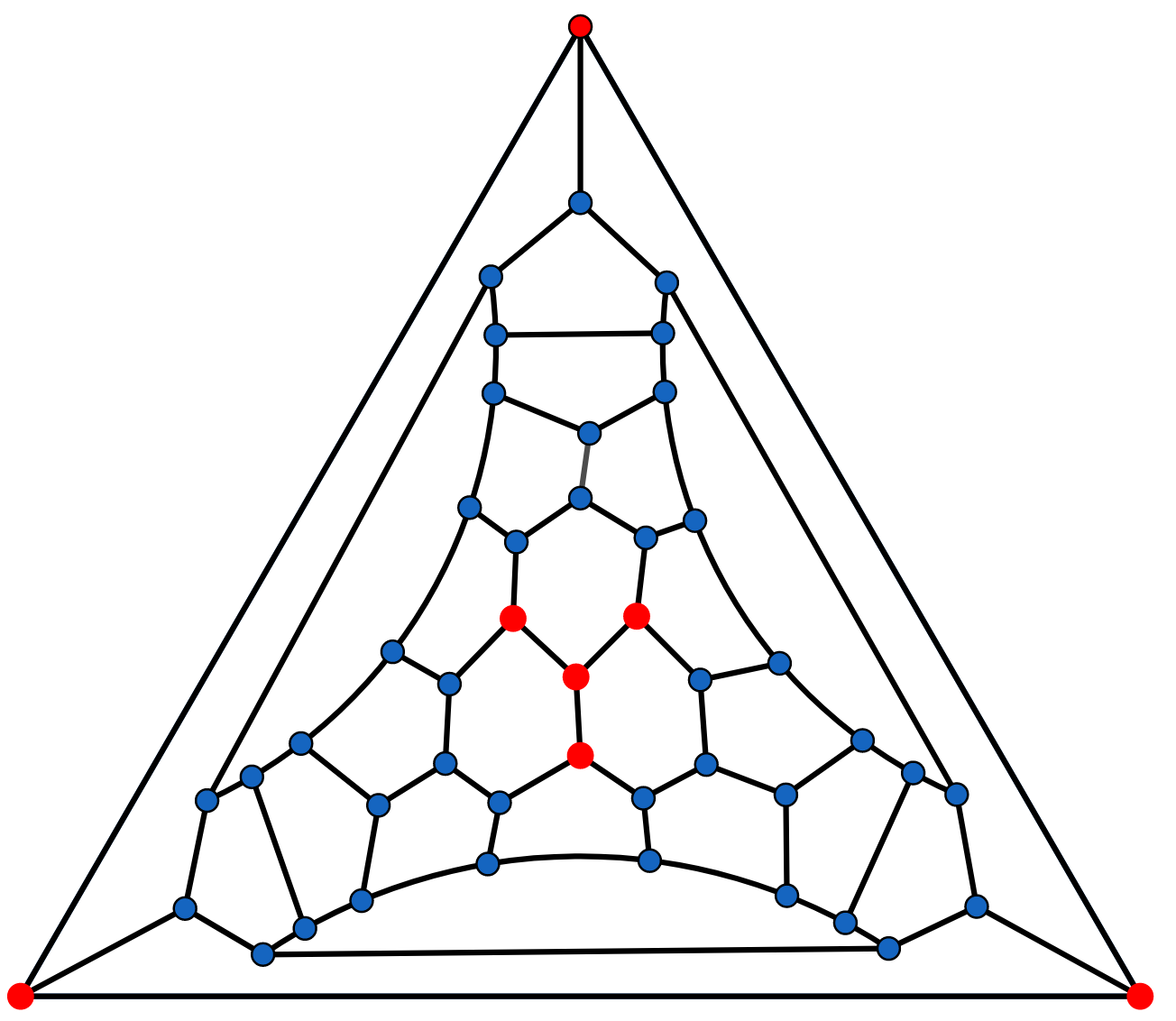
(b)

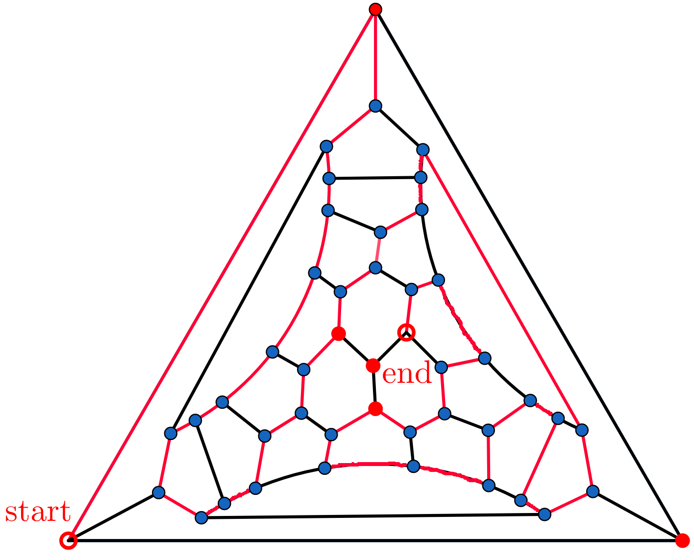
(c)

Figure 1.2: (a) The planar 3-regular Grünbaum graph of a simple 3-polytope that is not Hamiltonian, nor line-Hamiltonian. (b) Simplification of the Grünbaum graph. (c) Spanning path of the Grünbaum graph implying line-Hamiltonian path.

Proof.

By Balinski’s theorem, graphs of $d$-polytopes are $d$-connected, and so are their line graphs. Chen, Lai, Lai, and Weng [12] proved in 1993 that if a connected graph $G$ does not have vertices of degree 3 and its line graph $L(G)$ is $4$-connected, then $L(G)$ is Hamiltonian. This immediately implies that the graphs of all $d$-polytopes are line-Hamiltonian for $d\geq 4$. (The same result would also follow from a 2012 paper of Broersma, Ryjáček, and Vrána [9, Corollary 30], and for polytopes of dimension $5$ or more, from Kaiser-Vrana’s 2012 result that every $5$-connected line graph with minimum degree $\geq 6$ is Hamiltonian [21], as the line graph of the graph of a $d$-polytope has minimum degree $\geq 2d$.)

The smallest polytopal graph for which we were able to exclude the line-Hamiltonian property, is the planar 3-regular Grünbaum graph $H$ in Figure 1.2a, on 124 vertices. Every line-Hamiltonian cycle has to visit any of the small triangles exactly once since the graph is 3-regular. The graph $G$ in Figure 1.2b is constructed from $H$ by replacing each of the small triangles with a blue vertex; the remaining vertices stay and are colored red. Thus $G$ is line-Hamiltonian if and only if there is a Hamiltonian subgraph in $H$ that contains all the blue points and a suitable combination of the red points. However, with a computer check via sage, we verified that no such subgraph of $H$ exists. Thus $G$ is not line-Hamiltonian; Figure 1.2c shows however that it is line-traceable.

It remains to construct a simple 3-polytope that is neither line-Hamiltonian nor line-traceable. In the hope of getting an example as small as possible, we start with Zamfirescu’s graph $Z$ from Figure 1.3a; this is the graph of a simple 3-polytope on 88 vertices which is itself not traceable. We replace all but the six red vertices with triangles and denote this new graph $\tilde{Z}$. We claim that this cannot be line-traceable. In fact, each of the three blocks has only three edges coming out of it: toward the left, right, and middle; as illustrated in Figure 1.3b. Hence each block can be passed through only once by any spanning path of $\tilde{Z}$. Moreover, the center triangle of $\tilde{Z}$ can be passed through only once. From these observations, it is clear that any spanning path of $\tilde{Z}$ has to pass through at least one of the blocks in one go either from left to right or from the middle to right. A spanning path of $\tilde{Z}$ would correspond then to a simple path in $Z$ that meets every black vertex exactly once and may or may not pass through the red vertices. However, with a computer check via sage, we verified that there is no spanning path of the block going from left to right nor from the middle to right, regardless of which of the red vertices we include. ∎

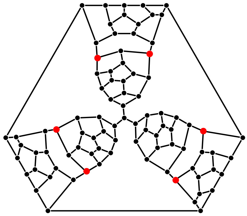
(a)

(b)

Figure 1.3: (a) Zamfirescu’s $3$-regular graph is not traceable, but it is line-traceable, but non-traceable. It can be modified by replacing all but the six red vertices with triangles into a non-line-traceable graph of a simple 3-polytope with 252 vertices. (b) A block of the simple 3-polytope with non-line-traceable graph with 252 vertices.

Next, we wish to produce $3$-polytopes whose graph is far from line-traceable. Following the notation in [18], let $p(G)$ be the maximal length of a simple path in $G$. For each $n$, Grünbaum and Motzkin constructed a graph $G^{n}$ of a simple 3-polytope with $n$ vertices and $p(G^{n})<2n^{\alpha}$ for some $\alpha<1$ (e.g., $\alpha=1-2^{-19}$) [18]. Adapting their proof, we show:

Proposition 5.

For any $n$, there is a graph $G^{\Delta}$ of a simple 3-polytope on $3n$ vertices with $p(L(G^{\Delta}))<10n^{\alpha}$, where $\alpha<1$ (e.g., $\alpha=1-2^{-19}$).

Proof.

For fixed $n$, let us denote by $G^{n}$ the Grünbaum–Motzkin graph of a simple 3-polytope with $n$ vertices for which $p(G^{n})<2n^{\alpha}$ from [18]. Since each vertex has degree 3, we can replace each vertex of $G_{n}$ with a triangle, without destroying 3-regularity. Let us denote the resulting graph by $G^{\Delta}_{n}$. Since $G^{\Delta}_{n}$ is 3-regular, every path (even not a simple one) can pass through each triangle only once. Now say we have a path $p$ in $G^{n}$ of length $p(G^{n})=m$. The corresponding path in $G^{\Delta}_{n}$ spans a subgraph with at most 4 edges for each interior vertex of $p$, the original $(m-1)$ edges, and 2 edges for the boundary vertices (edges of the boundary vertices cannot lead to a new vertex, else we could extend $p$), see Figure 1.4. We can conclude

$$p(L(G^{\Delta}_{n}))\leq 4(m-2)+(m-1)+2\cdot 3=5m-3<5(2n^{\alpha})-3<10n^{\alpha}\ .\qed$$

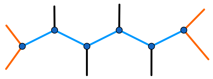
(a)

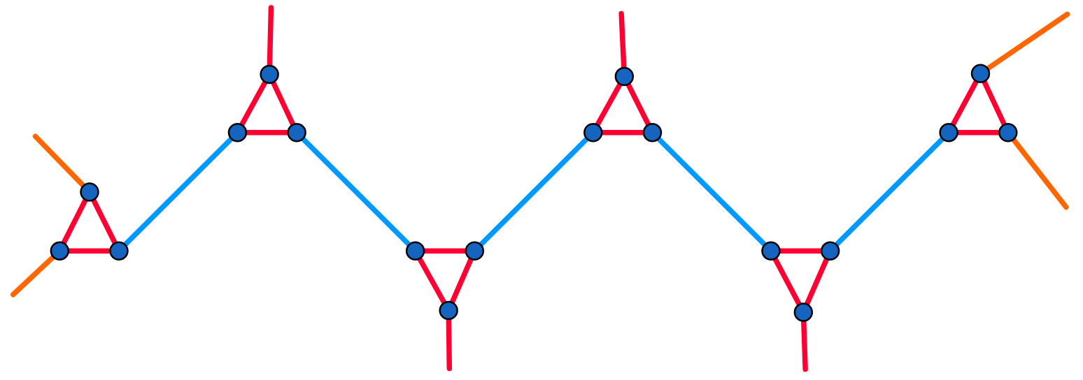
(b)

Figure 1.4: (a) Blue edges represent a path $p$ of maximal length in a Grünbaum–Motzkin graph $G^{n}$. The yellow edges cannot lead to a new vertex, or else $p$ would not be maximal. (b) The corresponding path in $G^{\Delta}_{n}$ spans a subgraph with $\leq 4$ edges for each interior vertex of $p$ (in red), plus the original $m-1$ edges (in blue), plus 2 edges for the boundary vertices (in red).

Remark 6.

Moon and Moser [28] also constructed a family of 3-polytopes that improves on Grünbaum and Motzkin’s bound for large values of $n$ [28]. However, it turns out that all the Moon–Moser polytopes have line-Hamiltonian graph, a fact which highlights the non-triviality of Proposition 5. To prove this fact, let us briefly recall their construction. We start with a tetrahedron $G_{0}$, and call its vertices and edges “the 0th stage vertices and edges”. To each boundary triangle of $G_{0}$, we attach a new tetrahedron. Let $G_{1}$ be the resulting polytope $G_{1}$; it has 12 boundary triangles, 4 new vertices (which we call “1st stage vertices”), and 12 new edges (the “1st stage edges). We repeat until reaching, say, $G_{k}$. In the graph of $G_{k}$, as we zoom in into one of the tetrahedra from the stage $(k-1)$, say $\Delta$, we see the three new tetrahedra attached to it, see Figure 1.5a. In this subgraph, we can always find a cycle visiting all its vertices of the $k$-th stage using only the edges of the $k$-th stage and passing through the vertex of $\Delta$ where all the three attached tetrahedra meet. Since a spanning cycle can pass through a vertex multiple times (depending on its degree), from these small cycles we get inductively a spanning cycle of the whole graph, see Figures 1.5b, 1.5c. This shows that all Moon–Moser graphs are line-Hamiltonian, even if they are far from being traceable.

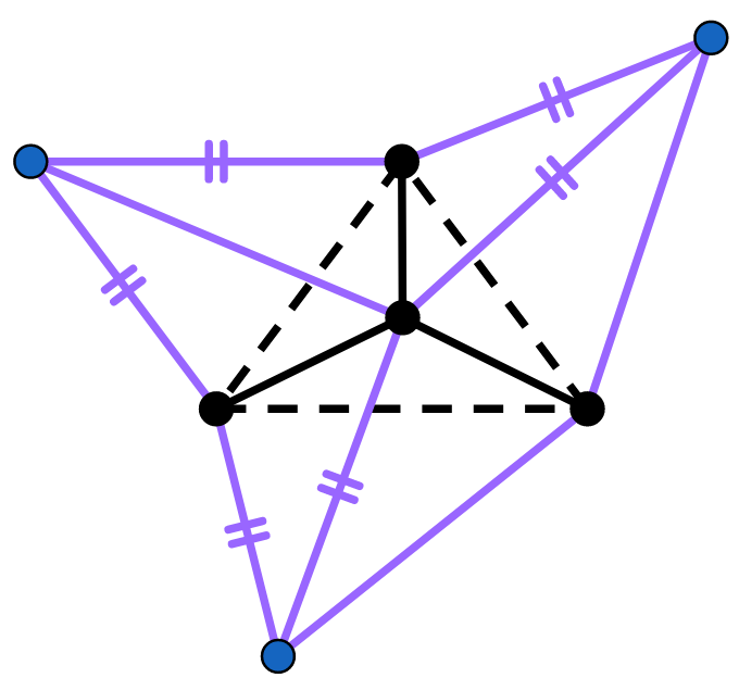
(a)

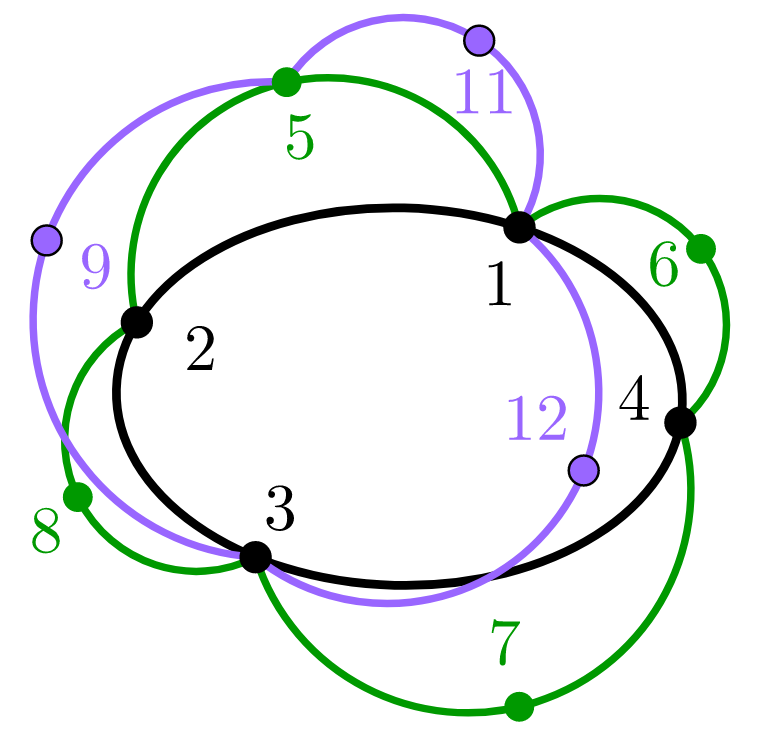
(b)

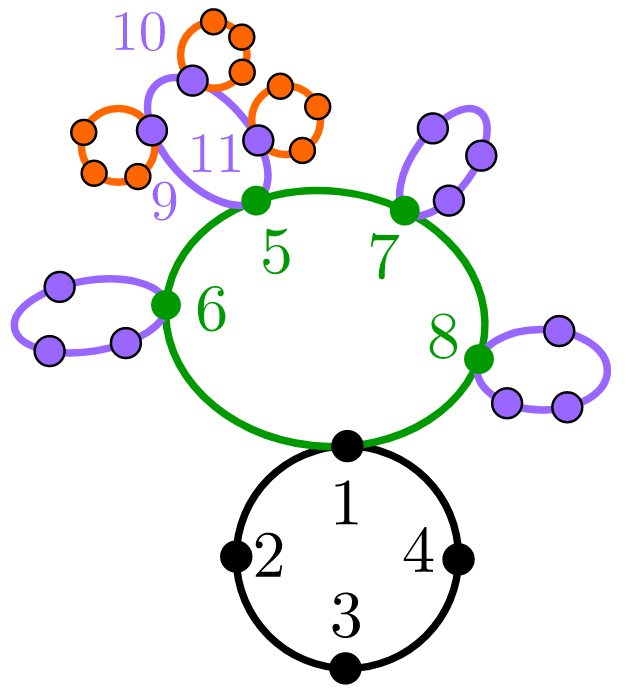
(c)

Figure 1.5: The Moon–Moser construction: (a) Zooming in on one of the $(k-1)$-st stage tetrahedra, whose vertices and edges are in black. The $k$-th stage vertices and edges are in purple. A cycle meeting all the new vertices that uses only new edges and passes through the vertex common to all three new tetrahedra is indicated by dashes on its edges. (b) Inductively, we get cycles at each stage that do not repeat edges. Here we show cycles in stages 0, 1, and one cycle (out of four) in stage 2. (c) To illustrate the spanning cycle, we remove all unnecessary intersections from the picture.

As a conclusion to this section, we should mention that both Balinski’s theorem and its equivalent dual formulation (“dual graphs of $d$-polytopes are $d$-connected”) have been extended beyond the world of polytopes:

Definition 7.

A $d$-pseudomanifold is a strongly-connected $d$-dimensional polytopal complex where every $(d-1)$-face lies in exactly $2$ facets.

Proposition 8 (essentially Barnette).

The graph and the dual graph of every $d$-pseudomanifold are both $(d+1)$-connected.

For the ‘graph’ part, Proposition 8 was first proven by Barnette [3]. For dual graphs of simplicial pseudomanifolds, the connectedness result above is proven by Klee [25], yet his proof argument works only for the simplicial case. Later Barnette published another special proof of Proposition 8, valid only for $d$-dimensional homology manifolds [2]. Since we were not able to find in the literature a proof of Proposition 8 valid in the full generality of (polytopal) pseudomanifolds, for completeness we provide one below.

Definition 9.

Let $P$ be a $d$-pseudomanifold. By a path of $d$-faces connecting $F^{\prime}$ and $F^{\prime\prime}$ in $P$ we mean a sequence $F_{1},\ldots,F_{s}$ of $d$-faces of $P$ such that $F_{1}=F^{\prime}$, $F_{s}=F^{\prime\prime}$, and for each $i\in\{1,\ldots,s-1\}$ the intersection $F_{i}\cap F_{i+1}$ is $(d-1)$-dimensional. We say that two paths of faces connecting $F^{\prime}$ and $F^{\prime\prime}$ are interior-disjoint if they do not have $d$-faces in common other than $F^{\prime}$ and $F^{\prime\prime}$. Finally, a cycle of $d$-faces is a path where first and last facet coincide.

Lemma 10 (Barnette, [3, Lemma 1]).

Let $P$ be a $d$-pseudomanifold. Let $S$ and $T$ be two $d$-faces that share a $(d-2)$-face $\sigma$. Then in $P$ there is a cycle of $d$-faces all containing $\sigma$.

Proof.

See Barnette [3, Lemma 1]. ∎

Proof of Proposition 8.

Let $X$ be a collection of at most $d$ facets in the $d$-pseudomanifold. Let $F^{\prime}$ and $F^{\prime\prime}$ be two facets not in $X$. Let $F^{\prime}=F_{1},F_{2},\ldots,F_{s}=F^{\prime\prime}$ be a path of $d$-faces that crosses as few elements of $X$ as possible. We claim that such a path must avoid $X$ altogether. In fact, suppose not. Let $G$ be the first $d$-face from $X$ that we encounter along the path. Note that the path features three consecutive $d$-faces $F,G,H$, with $F\notin X$ and $G\in X$. Since the dual graph of $G$ is $d$-connected (by Balinski’s theorem), in $\partial G$ between $\sigma\mathrel{\overset{\makebox[0.0pt]{\mbox{\tiny def}}}{=}}(F\cap G)$ and $\tau\mathrel{\overset{\makebox[0.0pt]{\mbox{\tiny def}}}{=}}(G\cap H)$ there are $d$ interior-disjoint paths of $(d-1)$-faces. But any path of $(d-1)$-faces in $\partial G$ is the restriction to $\partial G$ of a sequence of facets of $P$ adjacent to $G$, each intersecting the previous one in codimension $1$ or $2$. We claim that any such sequence can be completed to a path of $d$-faces connecting $F$ and $H$. In fact, let $S$ and $T$ be any two consecutive $d$-faces in the sequence with $\dim(S\cap T)=d-2$. By Barnette [3, Lemma 1] there is a cycle of $d$-faces that all contain $S\cap T$; adding to our sequence the portion of the cycle that does not contain $G$, we can ‘fill in the gap’ between $S$ and $T$ in the dual graph of $P$. So the claim is proven. Moreover, all $d$-faces we insert when we fill in gaps have $(d-2)$-dimensional intersection with $G$. In particular, no face $U$ can be used to fill in two different gaps between different pairs of facets, or else $U\cap G$ would contain two distinct $(d-2)$-faces, and thus it would have to be $(d-1)$-dimensional. We conclude that there exist $d$ interior-disjoint paths of $d$-faces connecting $F$ to $H$ and avoiding $G$. But since $|X\setminus\{G\}|<d$, at least one of these $d$ paths does not contain elements of $X$ other than (possibly) $H$. Using this path to bypass $G$, we can modify $F_{1},F_{2},\ldots,F_{s}$ to obtain another path of $d$-faces that features fewer elements of $X$. This contradicts how the path $F_{1},F_{2},\ldots,F_{s}$ was chosen. ∎

Proposition 11.

Let $d$ be a positive integer.

• All graphs and all dual graphs of $d$-pseudomanifolds are line-Hamiltonian if and only if $d\neq 2$.

• All graphs of flag simplicial $d$-pseudomanifolds are line-Hamiltonian.

• All dual graphs of subspace arrangements defined by an ideal $I$ such that $S/I$ is Gorenstein and has regularity $d+1$ are line-Hamiltonian if $d\geq 3$, and the bound is sharp.

Proof.

Every $1$-pseudomanifold is a cycle, so both its graph and its dual graph are trivially Hamiltonian. Barnette [3] showed that the graph of every $d$-pseudomanifold is $(d+1)$-connected; see Proposition 8 for the dual result. Athanasiadis [1] proved that the graph of every flag simplicial $d$-pseudomanifold is $2d$-connected, for $d\geq 2$; cf. also [7]. Benedetti–Varbaro [5] showed that if $I\subseteq S=\mathbb{K}[x_{1},\ldots,x_{n}]$ is an ideal defining a subspace arrangement, with $S/I$ Gorenstein of Castelnuovo–Mumford regularity $d+1$, the dual graph of the arrangement is $(d+1)$-connected. These four results, paired with Chen–Lai–Lai–Weng’s theorem [12], imply the line-Hamiltonian property as in the proof of Proposition 4, if $d$ is within the bounds described for each case. As for the sharpness of such bounds, the Grünbaum graph $H$ from Figure 1.2a is the graph of a simple $3$-polytope $P$, whose boundary complex is a polyhedral 2-sphere with graph $H$. The boundary complex $C$ of the dual polytope of $P$ is a simplicial $2$-pseudomanifold with dual graph $H$. If $I_{C}$ is the Stanley–Reisner ideal of $C$, then $S/I_{C}$ is Gorenstein of regularity $3$, and the dual graph to $I_{C}$ is still $H$ [5]. ∎

2 Four examples of non-Hamiltonian complexes

There are three ways in the literature to extend to $d$-dimensional complexes the notion of “Hamiltonian graph”; we recall them below:

Definition 12.

Let $\Sigma^{d}_{n}$ be the $d$-skeleton of the $(n-1)$-simplex, with vertices labeled by $1,\ldots,n$. Let $\,H_{i}$ be the $d$-face of $\Sigma^{d}_{n}$ with vertices $i,i+1,i+2,\ldots,i+d$, where the sum is taken modulo $n$. We say that a $d$-dimensional simplicial complex $\Delta$ on vertex set $\{1,\ldots,n\}$

• admits a tight-Hamiltonian path (resp. cycle) if it has a vertex labeling such that all of $H_{1},\dots,H_{n-d}$ (resp. all of $H_{1},\dots,H_{n}$) are in $\Delta$.

• admits a weakly-Hamiltonian path (resp. cycle) if it has a vertex labeling such that $\Delta$ contains faces $H_{i_{1}},\dots,H_{i_{k}}$ from the set $\{H_{1},\dots,H_{n-d}\}$ that altogether cover all the vertices, and such that $H_{i_{j}}$ is incident to $H_{i_{j+1}}$ for each $j\in\{1,\dots,k-1\}$ (respectively: for each $j\in\{1,\dots,k\}$, where by $i_{k+1}$ we mean $i_{1}$).

• admits a loose-Hamiltonian path (resp. cycle) if it admits a weakly-Hamiltonian path (resp. cycle) with all of the intersections $H_{i_{j}}\cap H_{i_{j+1}}$ consisting of a single point, except possibly for one exception, where the intersection may be larger.

Moreover, we say that $\Delta$ is maximally non-tight-Hamiltonian (resp. maximally non-weakly-Hamiltonian) if it does not admit any tight-Hamiltonian (resp. weakly-Hamiltonian) cycles, yet for any “missing $d$-face” $\sigma\in\Sigma^{d}_{n}$, $\sigma\notin\Delta$, the $d$-complex $\Delta^{\prime}=\Delta\cup\sigma$ does admit some tight-Hamiltonian (resp. weakly-Hamiltonian) cycle.

The last definition echoes the following classical one: a graph $G$ is maximally non-Hamiltonian if $G$ is not Hamiltonian, yet for any $x,y$ not adjacent in $G$, the graph $G$ + $[x,y]$ is Hamiltonian. Clearly, any maximally non-Hamiltonian graph has a Hamiltonian path. This trick is used in the proofs of Posa’s [30] and Chvátal’s theorem [13]; see also [14, 15, 26, 32].

Proposition 13.

For any integer $d\geq 2$, there is a $d$-dimensional simplicial complex $D_{d}$ without (tight, loose, or weak) Hamiltonian paths in which any of the $n=2d+2$ vertices is in at least $\binom{2d}{d-1}>\frac{n}{2}$ facets. Moreover, $D_{2}$ is maximally non-weakly-Hamiltonian.

Proof.

Let $D_{d}=v\ast\Sigma^{d-1}_{2d+1}$. This $D_{d}$ is a $d$-complex on $n=2d+2$ vertices. The vertex $v$ is present in all facets, by construction. Any other vertex is in $\binom{2d}{d-1}$ facets, which is larger than $d+1$ for $d\geq 2$. So every vertex has degree $>\frac{n}{2}$. Suppose by contradiction that $D_{d}$ admits a weakly-Hamiltonian path or cycle. Such path/cycle must be formed by facets $H_{i}$’s that all contain the vertex $v$. At the same time, if $k\in\{1,\ldots,n\}$ is the label assigned to vertex $v$, the only facets $H_{i}$ that contain $k$ are $H_{k},H_{k-1},\ldots,H_{k-d}$: These are $d+1$ faces that altogether cover $2d+1$ vertices, namely, those with a label between $k-d$ and $k+d$. But our complex $D_{d}$ has $n=2d+2$ vertices, so at least one of its vertices is not covered by the weakly-Hamiltonian path/cycle. A contradiction. Finally, we verified with the software [29] that adding any ‘missing triangle’ to $D_{2}$ produces a weakly-Hamiltonian cycle. ∎

The computational approach above, which proved $D_{d}$ maximally non-weakly-Hamiltonian for $d=2$, is of course not available for larger or arbitrary $d$. The next proposition however showcases an even simpler example that works in all dimensions:

Proposition 14.

Let $d$ be a positive integer. Any $d$-complex that is maximally non-tight Hamiltonian must admit tight Hamiltonian paths; if $d\geq 2$, it must also admit loose-Hamiltonian cycles. In contrast, for any integer $d\geq 2$, there is a $d$-dimensional simplicial complex without (tight, loose, or weak) Hamiltonian paths that is maximally non-weakly-Hamiltonian.

Proof.

The first part is easy and left to the reader. For the second part, let $W^{d}$ be the join of $3$ disjoint points with the $(d-1)$-simplex. It is easy to see that the $d$-complex $W^{d}$ does not have (tight, loose, or weak) Hamiltonian paths, cf. [4]. Let us prove that $W^{d}$ is maximally non-weakly-Hamiltonian. We label the vertices of the $(d-1)$-simplex by $1,\ldots,d$. Let us call “apices” the vertices $d+1,d+2$, $d+3$. Let $F\in\Sigma^{d}_{d+3}$. There are 3 cases:

1. If $F$ contains exactly $1$ apex, then $F$ already belongs to $W^{d}$.

2. If $F$ contains exactly $2$ apices, then up to permuting the labels of the first $d$ vertices and the labels of the last $3$ we can assume that $F=[1,2,\ldots,d-1,d+2,d+3]$. Hence $W^{d}\cup F$ admits a weak Hamiltonian cycle formed by the three faces $H_{1},H_{d+3},F$.

3. If $F$ contains $3$ apices, up to relabeling $F=[1,2,\ldots,d-2,d+1,d+2,d+3]$. (When $d=2$, $F=[d+1,d+2,d+3]$.) So $W^{d}\cup F$ admits the weak cycle $H_{1},H_{d+3},F$. ∎

Our next example shows that Chvátal’s famous result that “all self-complementary graphs are traceable” [13] does not extend to higher dimensions either. Recall that a pure $d$-dimensional complex $S$ on $n$ vertices is called self-complementary if it is combinatorially equivalent to the pure $d$-complex whose facets are the $d$-faces of $\Sigma^{d}_{n}$ that are not in $S$.

Proposition 15.

There exists a self-complementary $2$-complex without (tight, loose, or weak) Hamiltonian paths.

Proof.

Consider the $2$-dimensional complex

$$S=[1,3,5],[2,3,4],[1,2,4],[1,3,6],[1,2,5],[2,3,5],[1,4,5],[1,2,3],[1,2,6],[1,3,4].$$

This $S$ is self-complementary: it is isomorphic to its complement

$$S^{c}=[1,4,6],[1,5,6],[2,3,6],[2,4,5],[2,4,6],[2,5,6],[3,4,5],[3,4,6],[3,5,6],[4,5,6]$$

via the map $1\rightarrow 6$, $2\rightarrow 5$, $3\rightarrow 4$, $4\rightarrow 2$, $5\rightarrow 3$, $6\rightarrow 1$. Yet we verified with the software [29] that $S$ has no (tight, loose, or weak) Hamiltonian paths. ∎

Remark 16.

As a curiosity, $S$ is also a counterexample to the generalization of other two well-known graph-theoretical statements: In fact, we verified with [29] that $S$ admits weakly Hamiltonian cycles but not weakly Hamiltonian paths, whereas all Hamiltonian graphs are traceable; moreover, $S$ is under-closed but not chordal, cf. [4], whereas all interval graphs are chordal.

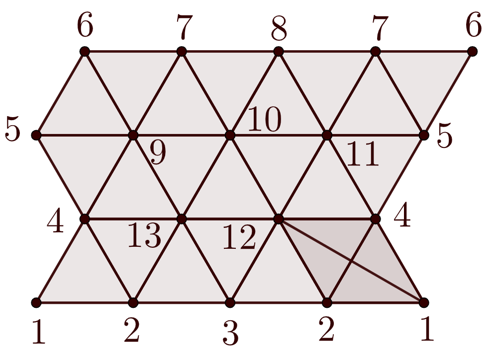
Figure 2.1: A 2-strongly-connected 2-complex $K$ whose square has no Hamiltonian cycles.

Finally, recall that the square $G^{2}$ of a graph $G$ is the graph obtained from $G$ by adding an edge $[i,j]$ for every two non-adjacent vertices $i,j$ of $G$ that are connected in $G$ by a $2$-edge path. Fleischner showed that if $G$ is $2$-connected, then $G^{2}$ is Hamiltonian [17].

Definition 17.

Given a $d$-complex $C$, let us define its square $C^{2}$ as the $d$-complex obtained from $C$ by adding any $d$-face that would be introduced via any possible bistellar flip that does not add vertices.

For example, if $C=[1,2,3],[2,3,4],[3,4,5]$, then flipping at $[2,3]$ would introduce triangles $[1,3,4]$ and $[1,2,4]$, whereas flipping at $[3,4]$ would introduce $[2,3,5]$ and $[2,4,5]$; so $C^{2}$ is obtained adding to $C$ the 4 triangles $[1,2,4],[1,3,4],[2,3,5],[2,4,5]$. Clearly, this notion of “square of a $d$-complex” boils down for $d=1$ to the square of a graph.

Proposition 18.

There exists a $2$-dimensional simplicial complex $K$ that is strongly-connected, and remains strongly-connected after the deletion of any vertex; yet its square $K^{2}$ does not admit (tight, loose, or weak) Hamiltonian cycles.

Proof.

Consider the $2$-dimensional complex of Figure 2.1,

$$\begin{array}[]{ll}K=&[2,4,12],\;[1,2,4],\;[1,2,12],\;[1,4,12],\;[2,4,13],\;[2,3,13],\;[3,12,13],\;[2,3,12],\\ &[4,5,9],\;[4,9,13],\;[9,10,13],\;[10,12,13],\;[10,11,12],\;[4,11,12],\;[4,5,11],\\ &[5,6,9],\;[6,7,9],\;[7,8,10],\;[7,8,11],\;[5,6,7],\;[5,7,11],\;[7,9,10],\;[8,10,11].\end{array}$$

This $K$ is “$2$-strongly-connected”, meaning that any complex obtained from $K$ by deleting at most one vertex, however chosen, is strongly-connected. The square $K^{2}$ is obtained by adding 46 more triangles. Despite the large size, it can be verified with the software [29] that $K^{2}$ does not have (tight, loose, or weak) Hamiltonian cycles. ∎

References

- [1] C. A. Athanasiadis, Some combinatorial properties of flag simplicial pseudomanifolds and spheres, Ark. Mat. 49 (1) (2011), 17–-29.
- [2] D. Barnette, Decompositions of homology manifolds and their graphs, Israel Journal of Mathematics 41 (1982), 203–212.
- [3] D. Barnette, Graph theorems for manifolds, Israel Journal of Mathematics 16 (1973), 62–72.
- [4] B. Benedetti, L. Seccia, and M. Varbaro, Hamiltonian paths, unit-interval complexes, and determinantal facet ideals, Advances in Applied Mathematics, in press.
- [5] B. Benedetti and M. Varbaro, On the Dual Graphs of Cohen–Macaulay Algebras, International Mathematics Research Notices, 2015 (17) (2015), 8085–8115.
- [6] A. A. Bertossi, Finding Hamiltonian circuits in proper interval graphs, Inf. Proc. Lett. 17 (1983), 97–101.
- [7] A. Björner and K. Vorwerk, On the Connectivity of Manifold Graphs, Proceedings of the American Mathematical Society 143 (2015), 4123–4132.
- [8] G. Brinkmann and B. McKay, Combinatorial Data, Plane Graphs, available at http://users.cecs.anu.edu.au/~bdm/data/planegraphs.html.
- [9] H. J. Broersma, Z. Ryjáček, P. Vrána How Many Conjectures Can You Stand? A Survey, Graphs and Combinatorics 28 (2012), 57–75.
- [10] G. Chartrand, On Hamiltonian line graphs, Transaction of the American Mathematical Society 134 (1968), 559–566.
- [11] C. Chen, C. C. Chang and G. J. Chang, Proper interval graphs and the guard problem, Discrete Mathematics 170 (1997), 223–230.
- [12] Z. Chen, H. Lai, H. Lai, and G. Weng, Jackson’s conjecture on Eulerian subgraphs, Combinatorics, graph theory, algorithms, and applications in Beijing (1993), 53–58.
- [13] V. Chvátal, On Hamilton’s Ideals, Journal of combinatorial theory 12(B), (1972), 163–168.
- [14] L. Clark and R. Entringer, Smallest maximally non-Hamiltonian graphs, Periodica Mathematica Hungarica 14 (1983), 57–68.
- [15] L. Clark, R. Entringer, and H. D. Shapiro, Smallest maximally non-Hamiltonian graphs II, Graphs and Combinatorics 8 (1992), 225–231
- [16] G. A. Dirac, Some theorems on abstract graphs, Proc. London Math. Soc. (1952), 69–81.
- [17] H. Fleischner, The square of every two-connected graph is Hamiltonian, Journal of Combinatorial Theory, Series 16(B), (1974), 29-–34.
- [18] B. Grünbaum and T. S. Motzkin, Longest simple paths in polyhedral graphs, J. London Math. Society 37 (1962), 152–160
- [19] H. Hán and M. Schacht, Dirac-type results for loose Hamilton cycles in uniform hypergraphs, Journal of Combinatorial Theory B 100 (2010), 332–346.
- [20] F. Harary and C. St. John Alva Nash-Williams, On Eulerian and Hamiltonian graphs and line graphs, Canad. Math. Bull. 8 (1965), 701–709.
- [21] T. Kaiser and P. Vrána, Hamilton cycles in 5-connected line graphs, European Journal of Combinatorics 33 (2012), 924–947.
- [22] R. M. Karp, Reducibility Among Combinatorial Problems, Complexity of Computer Computations (1972), 85–103.
- [23] G. Y. Katona and H. A. Kierstead, Hamiltonian chains in hypergraphs, J. Graph Theory 30 (1999), 205–212.
- [24] P. Keevash, D. Kuhn, R. Mycroft and D. Osthus, Loose Hamilton cycles in hypergraphs, Discrete Mathematics 311 (2011), 544–559.
- [25] V. Klee, A d-pseudomanifold with vertices has at least d- -simplices, Houston Journal of Mathematics 1 (1975), 81–86.
- [26] H. Kronk, A generalization of a theorem of Pósa, Proc. Amer. Math. Soc. 21 (1969), 77–78.
- [27] D. Kuhn and D. Osthus, Loose Hamilton cycles in 3-uniform hypergraphs of high minimum degree, Journal of Combinatorial Theory, Series B 96 (2006), 767–821.
- [28] J. W. Moon and L. Moser, Simple paths on polyhedra, Pacific J. Math. 13 (1963), 629–631.
- [29] M. Pavelka, A software for detecting closure properties in simplicial complexes, available at https://www.math.miami.edu/~pavelka/scpc/ (2021).
- [30] L. Pósa, A theorem concerning Hamilton lines, Magyar Tud. Akad. Mat. 7 (1962), 225–226.
- [31] V. Rodl, E. Szemerédi, and A. Ruciński, An approximate Dirac-type theorem for k-uniform hypergraphs, Combinatorica 28 (2008), 229–260.
- [32] P. V. Roldugin, Construction of maximally non-Hamiltonian graphs, Discrete Math. Applications 13 (2003), 277–289.
- [33] P. G. Tait, Remarks on the coloring of maps, Proc. Roy. Soc. Edinburgh 10 (1880), 501–503.
- [34] W. T. Tutte, On Hamiltonian circuits, J. London Math. Society 21 (1946), 98–101.