Dynamic Spanning Trees for Connectivity Queries on Fully-dynamic Undirected Graphs (Extended Version)

Abstract.

Answering connectivity queries is fundamental to fully dynamic graphs where edges and vertices are inserted and deleted frequently. Existing work proposes data structures and algorithms with worst case guarantees. We propose a new data structure, the dynamic tree (D-tree), together with algorithms to construct and maintain it. The D-tree is the first data structure that scales to fully dynamic graphs with millions of vertices and edges and, on average, answers connectivity queries much faster than data structures with worst case guarantees.

PVLDB Reference Format:
PVLDB, 15(11): XXX-XXX, 2022.
doi:XX.XX/XXX.XX

PVLDB Artifact Availability:
The source code, data, and/or other artifacts have been made available at

https://github.com/qingchen3/D-tree.

1. Introduction

The efficient processing of large graphs is becoming ever more important (see Hegeman and Iosup (Hegeman and Iosup, 2018), Sahu et al. (Sahu et al., 2017), and Sakr et al. (Sakr et al., 2021) for recent studies and surveys). A fundamental problem is the connectivity problem, which checks if there is a connection between two nodes in a graph. Answering connectivity queries plays a crucial role in application areas such as communication and transport networks, checking their reliability, as well as social networks, investigating the connections between users and the groups they belong to. However, it does not stop there: since dynamic connectivity is such a fundamental problem, we find applications in areas as diverse as computational geometry (Doraiswamy and Natarajan, 2009), chemistry (Eyal and Halperin, 2005), and biology (Henzinger et al., 1999).

Computing the connectivity between two nodes using search strategies like breadth-first search (BFS) and depth-first search (DFS) with a linear run-time is prohibitively expensive for large graphs with millions of vertices and edges. For static graphs, the connected components can be precomputed and the results stored in an auxiliary data structure, allowing the efficient processing of queries. Updating the auxiliary data structures in the fully dynamic case with frequent graph edge insertions and deletions is challenging, though. For instance, updating the well-known two-hop labeling (Zhu et al., 2014; Bramandia et al., 2009; Cohen et al., 2002; Lyu et al., 2021) is expensive, since BFS or DFS must be run on the graphs. Similarly, tree-based approaches (Frederickson, 1983; Henzinger and King, 1999; Holm et al., 2001; Thorup, 2000; Wulff-Nilsen, 2013; Huang et al., 2017) have focused on worst-case runtime guarantees and incur high update costs for large graphs. They rely on multiple complex auxiliary data structures, have often not been implemented and evaluated empirically (Alberts et al., 1997; Zaroliagis, 2002), and sacrifice average case performance to get an upper bound for the worst-case complexity. In our work, we focus on fully dynamic large real-world graphs with the goal of developing a connectivity algorithm with a good average case performance for queries and updates.

First, we define what optimizing the average case complexity for connectivity queries over the spanning forest (i.e., sets of spanning trees) of a graph means: the costs are minimized if $S_{d}$, the sum of distances between the root nodes and all the other nodes in the spanning trees, is minimized. Since maintaining a minimal $S_{d}$ in spanning trees in a fully dynamic setting is too expensive, we propose effective and practical heuristics to keep the value of $S_{d}$ of the spanning trees low. Our approach has a much better average runtime than solutions with a guaranteed worst case complexity for a broad range of real-word graphs (we demonstrate this empirically).

The most time-critical part is the search for a replacement edge when deleting an edge in a spanning tree. We prove that the cost for finding a replacement edge for an edge $e$ is proportional to the cut number of $e$, i.e., the number of nodes in the smaller tree after removing $e$ (deleting an edge splits a tree into two). Moreover, we prove that the average cost of finding a replacement edge is optimal for spanning trees that minimize $S_{c}$, the sum of the cut numbers for all possible edges in the spanning tree. We show that $S_{d}$ and $S_{c}$ are directly related to each other, i.e., optimizing one also optimizes the other.

Our main technical contribution can be summarized as follows:

• We formally define the problem of evaluating connectivity queries in fully dynamic graphs with an optimal average-case complexity.

• We introduce $S_{d}$ and $S_{c}$. $S_{d}$ is the sum of distances between roots and all other nodes; we show that the average cost of connectivity queries is optimal for spanning forests minimizing $S_{d}$. $S_{c}$ is the sum of cut numbers of all edges; we show that the average costs for finding replacement edges is optimal if spanning trees minimize $S_{c}$.

• We prove that $S_{d}=S_{c}$ for spanning trees in which the root is a centroid, i.e., a node that minimizes the sum of the distances to all other nodes, allowing us to optimize the average-case costs.

• We propose a novel k-ary tree, called dynamic tree (D-tree), to represent the connected components of a graph. We define D-trees and provide efficient, heuristics-based algorithms to answer connectivity queries and maintain D-trees when inserting and deleting edges.

• We embed the graph in a set of D-trees that also maintain edges not part of the spanning forest and the size of each subtree. This information helps us to keep the average runtimes of operations low.

• We conduct extensive experiments to compare D-trees with existing approaches over ten real-world datasets. The experiments confirm the efficiency of our approach and its superior average-case runtime.

2. Related Work

The first efficient connectivity algorithms focused on updating spanning trees in incremental (Tarjan, 1975) and decremental (Shiloach and Even, 1981) dynamic graphs, i.e., graphs only allowing insertions or deletions, respectively. The earliest algorithms for updating minimum spanning trees in fully dynamic undirected (weighted) graphs were developed by Spira and Pan (Spira and Pan, 1975), Chin and Houck (Chin and Houck, 1978), and Frederickson (Frederickson, 1983). The algorithm by Spira and Pan has a complexity of $O(n)$ for insertions and $O(n^{3})$ for deletions, with $n$ being the number of vertices. Chin and Houck improve the complexity for deletions to $O(n^{2})$. Frederickson brings the complexity of insertions and deletions down to $O(\sqrt{m})$, with $m$ being the number of edges. Using a technique called sparsification, Eppstein et al. improve the complexity to $O(\sqrt{n})$ per update operation (Eppstein, 1992; Eppstein et al., 1997), but without providing an implementation.

Henzinger and King represent spanning trees via Euler tours (Tarjan and Vishkin, 1984), resulting in elegant merging and splitting of spanning trees (Henzinger and King, 1995, 1997, 1999, 2001). Storing, searching, and maintaining Euler tours efficiently is not trivial, though. Henzinger and King proposed the Euler Tour Tree (ET-tree) (Henzinger and King, 1995, 1999) that maps Euler tours to balanced binary trees (Alberts et al., 1997; Seidel and Aragon, 1996) and requires several auxiliary data structures (Henzinger and King, 1995, 1999) to keep track of information for Euler tours.

The work by Henzinger and King (Henzinger and King, 1995, 1999) sparked a whole line of research based on hierarchical forests for dynamic connectivity. We divide the algorithms into two groups: those that minimize the worst-case costs and those that optimize the amortized costs. We first look at worst-case costs for update operations. Interestingly enough, for sparse graphs, the algorithm by Frederickson (Frederickson, 1983) (and the improvement by Eppstein (Eppstein et al., 1997)) is still competitive. Kapron et al. (Kapron et al., 2013) proposed an algorithm with complexity $O(\log^{5}n)$, but it turned out that it can produce false negatives. In 2016, Kejlberg-Rasmussen et al. (Kejlberg-Rasmussen et al., 2016) improved the complexity to $O(\sqrt{\nicefrac{{n(\log\log n)^{2}}}{{\log n}}})$. Henzinger and King were the first to look at amortized costs and achieve polynomial logarithmic amortized complexity. Holm at al. (Holm et al., 2001) improved the bound by adding invariants to the hierarchical forests. Orthogonal data structures, such as local trees, lazy local trees, bitmaps, and a system of shortcuts (Wulff-Nilsen, 2013; Thorup, 2000; Huang et al., 2017), are introduced to improve the amortized complexity. The combination of these complicated data structures makes it difficult to implement (and evaluate) these algorithms. In fact, only Henzinger-King’s algorithm $HK$ (Henzinger and King, 1995, 1999) was fully implemented and evaluated (Zaroliagis, 2002; Alberts et al., 1997; Iyer et al., 2002) and is therefore our main contender.

Most existing work on labeling schemes (Zhu et al., 2014; Bramandia et al., 2009; Wei et al., 2018; Cheng et al., 2013; Jin et al., 2009) requires that input graphs are directed and/or DAGs, and consequently are generally not applicable to undirected graphs. A recent data structure for labeling, called DBL (Lyu et al., 2021), works for undirected graphs. However, DBL only supports insertions on graphs, and constructing DBL is expensive since it needs to run BFS on connected components.

3. Preliminaries

We consider undirected unweighted simple graphs $G(V,E)$ defined by a set of vertices $V$ and a set $E$ of edges (Gibbons, 1985; West et al., 2001). A graph is simple iff there is at most one edge $(u,v)\in E$ that connects a pair of vertices $u,v\in V$. We measure the size of a graph in the number of vertices it contains, which we denote by $|V|$. Given a graph $G(V,E)$, a path $P$ is a sequence of distinct vertices $(v_{1},v_{2},\dots,v_{n})$, $v_{i}\in V$, such that each pair of adjacent vertices in $P$, $v_{i}$ and $v_{i+1}$, are connected via an edge $(v_{i},v_{i+1})\in E$. The length $|P|$ of a path $P$ is defined by the number of edges in the path, i.e., for $P=(v_{1},v_{2},\dots,v_{n})$, $|P|=n-1$. If there is an additional edge between $v_{n}$ and $v_{1}$, then the sequence $(v_{1},v_{2},\dots,v_{n})$ forms a cycle. The diameter of a graph is the length of the longest shortest path between two vertices in the graph. A connected component $C(V^{\prime},E^{\prime})$ is a maximal subgraph of a graph $G(V,E)$, with $V^{\prime}\subseteq V,E^{\prime}\subseteq E$, in which all pairs of nodes are connected via a path.

Example 3.1.

Figure 1 shows a graph $G_{1}$ with two connected components $C_{1}$ and $C_{2}$.

(a) Component $C_{1}$

(b) Component $C_{2}$

Figure 1. $G_{1}=\{C_{1},C_{2}\}$ with components $C_{1}$ and $C_{2}$

A tree is an undirected graph in which any pair of vertices is connected by exactly one path. Thus, the vertices in a tree are all connected and the tree does not contain cycles. In a forest, any two vertices are connected by at most one path, which means that its connected components consist of trees. In a rooted tree, we designate one vertex as the root $r$ of the tree. By definition, $r$ has depth 0. The depth of any other vertex $v$ is determined by its (tree) distance $d_{T}$ to $r$, i.e., $d_{T}(r,v)$ is equal to the length of the path from the root to the vertex. The height of a tree is equal to the depth of the leaf node with the maximum depth. Given a rooted tree with root $r$, the ancestors, $anc(v)$, of a node $v\not=r$ ($r$ does not have any ancestors) are all the nodes on the path from $v$ to $r$ except $v$. The parent of $v$ is the node $u$ on this path with $depth(u)+1=depth(v)$. The children of $v$ are the nodes that have $v$ as a parent. The descendants, $desc(v)$, of $v$ are all nodes $u\not=v$ for which $v$ appears in the path from $u$ to $r$. The subtree rooted at $v$ consists of $v$ and all its descendants. The size of this subtree, denoted by $size(v)$, is measured in the number of nodes it includes. Given a connected component $C(V^{\prime},E^{\prime})$, a spanning tree $T=(V^{\prime},E_{T})$, with $E_{T}\subseteq E^{\prime}$, is a rooted tree containing all vertices of $C$. We use a spanning forest, consisting of a spanning tree for each component, for graphs with more than one component.

Example 3.2.

Figure 2 depicts spanning forest $F_{1}$ for graph $G_{1}$ from Figure 1. $F_{1}$ is made up of spanning trees $T_{1}$ and $T_{2}$ for components $C_{1}$ and $C_{2}$, respectively. The path from $\mathsf{n_{5}}$ to $\mathsf{n_{1}}$ is ($\mathsf{n_{5}}$, $\mathsf{n_{3}}$, $\mathsf{n_{1}}$); $anc(\mathsf{n_{5}})$ = $\{\mathsf{n_{1}},\mathsf{n_{3}}\}$; $desc(\mathsf{n_{3}})$ = $\{\mathsf{n_{5}}\}$; $depth(\mathsf{n_{3}})$ = 1 and $depth(\mathsf{n_{5}})$ = 2. The subtree rooted at $\mathsf{n_{3}}$ consists of $\mathsf{n_{3}}$ and its descendant $\mathsf{n_{5}}$, and the size of this subtree is 2.

(a) Spanning Tree $T_{1}$ for $C_{1}$

(b) Spanning Tree $T_{2}$ for $C_{2}$

Figure 2. Spanning forest $F_{1}=\{T_{1},T_{2}\}$ for $G_{1}$ with spanning trees $T_{1}$ and $T_{2}$ for components $C_{1}$ and $C_{2}$. The roots of the spanning trees are colored red.

Definition 3.3 (Vertex deviation and centroid).

Given a tree $T=(V^{\prime},E_{T})$, the vertex deviation $m(v)$ of a vertex $v\in V^{\prime}$ is the average distance of $v$ to all other nodes: $m(v)=\nicefrac{{1}}{{|V^{\prime}|}}\sum_{u\in V^{\prime}}d_{T}(v,u)$. A centroid (or vertex median) of $T$ is a vertex with minimal $m(v)$ for $T$ (Jordan, 1869; Zelinka, 1968).

A tree with an even number of vertices can have two centroids. In this case, the two centroids are adjacent to each other (Zelinka, 1968).

Example 3.4.

The centroid of $T_{1}$ in Figure 2(a) is $\mathsf{n_{1}}$ since the vertex deviation $m(\mathsf{n_{1}})=\nicefrac{{(1+1+1+2+2)}}{{6}}=\nicefrac{{7}}{{6}}$, which is minimal for this tree.

4. Problem Definition

We now formally define connectivity queries on graphs and formulate the challenges posed by dynamic graphs.

Definition 4.1 (Connectivity query).

Given a graph $G(V,E)$ and two vertices $u,v\in V$, the connectivity query $conn(u,v)$ returns True if there exists a path between $u$ and $v$ in $G$, and False otherwise.

Example 4.2.

Consider graph $G_{1}$ in Figure 1. The connectivity query $conn(\mathsf{n_{2}},\mathsf{n_{6}})$ returns True, as $\mathsf{n_{2}}$ and $\mathsf{n_{6}}$ are connected via $\mathsf{n_{1}}$ and $\mathsf{n_{4}}$ (and also via $\mathsf{n_{5}}$ and $\mathsf{n_{3}}$). The connectivity query $conn(\mathsf{n_{6}},\mathsf{n_{9}})$ returns False, because $\mathsf{n_{6}}$ and $\mathsf{n_{9}}$ are located in different components.

A naive approach for checking connectivity is to run a search algorithm, such as breadth-first search (BFS) or depth-first search (DFS), from one of the two vertices and test if the search finds the other node, which is prohibitively expensive for large graphs (it has complexity $O(|V|+|E|)$). For static graphs, we can determine all connected components of a graph, using BFS or DFS (see, e.g.,  (Hopcroft and Tarjan, 1973)), and then label the nodes with the ID of the component they belong to. Given two nodes, we then directly decide in constant time whether they are connected. Evaluating connectivity queries on dynamic graphs is a much more challenging scenario. We first formally define dynamic graphs:

Definition 4.3 (Fully dynamic graph).

In a fully dynamic graph $G_{d}(V,E)$, edges are inserted and deleted one at a time. We apply a sequence of update operations to a graph, $((t_{1},o_{1}),(t_{2},o_{2}),$ $(t_{3},o_{3}),\dots)$, where $t_{i}$ is a timestamp and $o_{i}$ is either an insertion ($E_{t+1}=E_{t}\cup(v_{i},v_{j})$) or a deletion ($E_{t+1}=E_{t}\setminus(v_{i},v_{j})$) of an edge.

Since we only deal with dynamic graphs from here on, we drop the subscript $d$ and refer to dynamic graphs as $G(V,E)$. Our implementation allows the insertion and deletion of isolated, i.e., unconnected vertices. However, since spanning trees consisting of a single node are trivial to handle, we restrict our description to edge insertions and deletions.

As we will see later, in the worst case the performance of deletion operations is especially problematic. We argue that these cases rarely occur in real-world graphs and that it is more important to consider the average-case complexity.

Before going into the implementation details of our approach, which is based on spanning trees, we explicitly define the problem we are solving in Definition 4.4 and then investigate important aspects of applying spanning trees to evaluate connectivity queries in fully dynamic graphs and show how we exploit these properties in the following section.

Definition 4.4 (Problem definition).

Find a data structure that in fully dynamic graphs, on average, allows us to (a) answer connectivity queries and (b) maintain the data structure efficiently.

5. Leveraging Spanning Trees

We first define the problem of evaluating connectivity queries with an optimal average-case complexity. Next, we introduce $S_{d}$, which optimizes average costs for connectivity queries, and $S_{c}$, which optimizes average costs for searching for replacement edges. Finally, we formally establish the relationship between $S_{c}$ and $S_{d}$. All proofs for the theorems and lemmas in this section are shown in the appendix.

5.1. Evaluating Queries

We use a spanning forest to answer connectivity queries $conn(u,v)$ by traversing the paths from $u$ and $v$ to the respective roots $r_{u}$ and $r_{v}$ of their spanning trees. If we end up at the same root, then $u$ and $v$ are located in the same component and are connected. If we reach different roots, they are not connected. The costs for evaluating a connectivity query $conn(u,v)$ via spanning trees is equal to the sum of distances of $u$ and $v$ to their roots: $d_{T}(r_{u},u)+d_{T}(r_{v},v)$.

Definition 5.1 (Sum of distances between root and its descendants).

Given a (spanning) tree $T=(V^{\prime},E_{T})$ with root $r$, the sum of distances between $r$ and its descendants, $S_{d}$ is defined as follows:

(1) $$S_{d}(T)=\sum_{x\in V^{\prime}}d_{T}(r,x).$$

Before analyzing the average-case costs, we give a formal definition of these costs:

Definition 5.2 (Average-case complexity).

Let $I$ be the set of all possible inputs for an algorithm $A$ and let $t(i)$, $i\in I$, be the cost of running $A$ on input $i$. The probability that input $i$ occurs is defined by $p(i)$. The average cost of running $A$ is the expected value of the running times: $E(t)=\sum_{i\in I}t(i)p(i)$. If the probabilities $p(i)$ are not available, often a uniform distribution is assumed: $E(t)=\frac{1}{|I|}\sum_{i\in I}t(i)$.

A workload-aware analysis utilizing the probability distribution of the inputs is beyond the scope of this paper. In the following, we assume a uniform distribution of the inputs. We illustrate with an example what average-case versus worst-case costs mean for connectivity queries.

Example 5.3.

Consider the spanning tree $T_{1}$ in Figure 3(a). Then the worst case for evaluating a connectivity query occurs if we select $T_{1}.n_{19}$ and $T_{1}.n_{20}$ as parameters, leading to a cost of $3+3=6$. Assuming a uniform distribution of inputs for connectivity queries on $T_{1}$, we get $\nicefrac{{2*S_{d}(T_{1})}}{{|T_{1}|}}=\nicefrac{{(2*25)}}{{20}}=2.5$ for the average costs. If we balance the tree by rerooting it, we get $T^{\prime}_{1}$ as shown in Figure 3(b). For $T^{\prime}_{1}$ the costs are $4$ in the worst case and $3.5$ in the average case.

(a) Structure of $T_{1}$, $S_{d}$ = 25.

(b) Balanced trees $T^{\prime}_{1}$, $S_{d}$ = 35.

Figure 3. Unbalanced versus balanced spanning trees

In Example 5.3, by balancing the spanning trees (and optimizing the worst case), we actually worsen the average costs. Looking at $T_{1}$ in Figure 3(a), we can see that the paths from $n_{1}$ to $n_{19}$ and from $n_{1}$ to $n_{20}$ are outliers, all the other nodes are very close to $n_{1}$. In essence, balancing the tree punishes the performance of all other queries not involving these outliers. For this reason, other (tree-like) data structures, such as tries (Szpankowski, 1990) and multilevel extendible hashing schemes (Helmer et al., 2003), do not strive for balance, but allow the outlier parts to grow deeper than the rest of the tree.

We now investigate what spanning trees have to look like to guarantee minimum average costs.

Theorem 5.4.

The average costs of evaluating connectivity queries with spanning trees is optimal if the trees in the spanning forest minimize $S_{d}$.

Proof.

Shown in Appendix C.1. ∎

Generally, a high fanout leads to shallow trees (B-trees are a classical example), which in turn decreases the distances between the root and other nodes. When it comes to spanning trees, using breadth-first-search (BFS) trees provides excellent fanout, minimizing $S_{d}$ for a given root.

Definition 5.5 (Breadth-first-search tree (BFS-tree)).

For a connected component $C=(V^{\prime},E^{\prime})$ (or a connected graph), a BFS-tree is a spanning tree constructed by a breadth first search, which traverses the component level by level, starting from the root node $r$ of the BFS-tree, then visiting all the nodes at a distance of one, at a distance of two, and so on.

Example 5.6.

Shown in Appendix A.1

Lemma 5.7.

In a BFS-tree with root $r$ the sum of distances $S_{d}$ between $r$ and all other nodes is minimal.

Proof.

Shown in Appendix C.2 ∎

So, we could compute the optimal BFS-tree for each component, i.e., if $P=\{\mbox{BFS-tree with root }v|v\in V^{\prime}\}$ is the the set of all BFS-trees with different roots for component $C=(V^{\prime},E^{\prime})$, we select the tree with $S_{d}=\min_{T\in P}S_{d}(T)$ . This optimizes the average cost of running connectivity queries via spanning trees. For fully dynamic graphs, it is too expensive to update these spanning trees while preserving them to be optimal BFS-trees. Instead, we switch to efficient heuristics, e.g., by picking a root that is a centroid.

5.2. Updating Spanning Trees

We distinguish two different types of edges in a connected component: those that belong to the current spanning tree representing the component, which we call tree edges, and those that do not, which we call non-tree edges.

Definition 5.8 (Tree and non-tree edges).

Consider a connected component $C(V^{\prime},E^{\prime})$ and a spanning tree $T=(V^{\prime},E_{T})$ for $C$. An edge $(u,v)\in E^{\prime}$ is a tree edge for $C$ if $(u,v)\in E_{T}$, and a non-tree edge for $C$ if $(u,v)\in E^{\prime}\setminus E_{T}$.

Example 5.9.

Consider component $C_{1}=(V_{1},E_{1})$ in Figure 1(a) and spanning tree $T_{1}$ for $C_{1}$ in Figure 2(a). In $E_{1}$, edges $(\mathsf{n_{2}},\mathsf{n_{5}})$, $(\mathsf{n_{3}},\mathsf{n_{6}})$ and $(\mathsf{n_{4}},\mathsf{n_{5}})$ are non-tree edges while all other edges are tree edges.

We first look at update operations that involve non-tree edges, which is the simpler case, and then move on to updates of tree edges. When we delete a non-tree edge $(u,v)$ in a connected component $C(V^{\prime},E^{\prime})$, this does not affect the spanning tree and we do not have to make any changes to it (we know that all vertices in $C$ are still connected via the tree edges). Even better, if the spanning tree is an (optimal) BFS-tree, it will remain an (optimal) BFS-tree, since taking away an edge from $C$ does not add any shortcuts between nodes that could lead to a better tree.

Inserting a new non-tree edge $(u,v)$, i.e., both, $u$ and $v$, are in the same component $C$, means that the current spanning forest for $G$ is still valid. So, if we are only interested in maintaining spanning trees for the components of $G$, we would not have to modify anything. However, inserting a non-tree edge can invalidate that a spanning tree is a BFS-tree. Assume that $depth(u)+1<depth(v)$, then $v$ (and possibly some of its ancestors) can be reached faster through $u$ than taking the existing path from $v$ to the root of the tree. We can fix this case. We define $\Delta=depth(v)-depth(u)$. We disconnect $v$ and $(\Delta-2)$ of its ancestors ($v$’s $(\Delta-2)$-nd ancestor and $v$ have a distance of $(\Delta-2)$) from the spanning tree, reroot this subtree to make $v$ the new root, and connect this subtree to $u$. The edge $(u,v)$ becomes a tree edge, while the edge previously connecting the $(\Delta-2)$-nd ancestor to the tree becomes a non-tree edge. We now have a spanning tree that is a BFS-tree again. Note that the heuristic does not guarantee the optimality of the BFS-tree.

Example 5.10.

Figure 4 shows an example of restoring a BFS-tree after inserting a non-tree edge ($\mathsf{n}_{5}$, $\mathsf{n}_{8}$). $\mathsf{n}_{5}$ can reach root $\mathsf{n}_{1}$ faster through $\mathsf{n}_{8}$. Since $depth(\mathsf{n}_{8})+1$ $<$ $depth(\mathsf{n}_{5})$, $\Delta$ = $depth(\mathsf{n}_{5})$ $-$ $depth(\mathsf{n}_{8})$ = $4-1$ = 3, and $\Delta-2$ = 1, the $(\Delta-2)$-nd ancestor of $\mathsf{n}_{5}$ is $\mathsf{n}_{4}$. We disconnect $\mathsf{n}_{4}$ from the tree, turning $\mathsf{n}_{5}$ into the root of the subtree and connecting this subtree to $\mathsf{n}_{8}$. The previous tree edge ($\mathsf{n}_{3}$, $\mathsf{n}_{4}$) becomes a non-tree edge (not shown in Figure 4) and ($\mathsf{n}_{5}$, $\mathsf{n}_{8}$) becomes a tree edge. While the tree in Figure 4(b) is a BFS-tree, it is not the BFS-tree with the optimal $S_{d}$ anymore. In Section 5.4 we show how to improve $S_{d}$.

(a) Inserting the (dashed) non-tree edge ($\mathsf{n}_{5}$, $\mathsf{n}_{8}$), $S_{d}$ = 27.

(b) After restoring the BFS-tree, $S_{d}$ = 23.

Figure 4. Restoring the BFS-tree.

Let us now turn to updates involving tree edges. If we insert a new edge $(u,v)$ into $G$ and discover that $u$ and $v$ are located in different components, $C_{1}$ and $C_{2}$, respectively, then we need to merge $C_{1}$ and $C_{2}$ into a single component $C_{3}$. Consequently, the spanning trees $T_{1}$ and $T_{2}$ currently representing $C_{1}$ and $C_{2}$ also need to be merged into a single spanning tree $T_{3}$. This involves rerooting one of the trees and connecting it to the other. Assume that we make $v$ the new root of $T_{2}$, which, w.l.o.g., is the smaller tree, and then connect it via $(u,v)$ to $T_{1}$, making $(u,v)$ a tree edge in $T_{3}$. If we start with trees that are BFS-trees, the part covered by $T_{1}$ will still be one and the edge $(u,v)$ is on the shortest path to connect to vertices in $T_{2}$, which may not be a BFS-tree anymore after the rerooting. Essentially, this limits the damage we do to the smaller tree. Instead of rerooting $T_{2}$, we could run BFS on $T_{2}$ starting at node $v$ (to recreate a BFS-tree) and then connect $u$ to $v$. This entails costs of $O(|V_{2}|+|E_{T_{2}}|)$, compared to $O(depth(v))$ for rerooting the tree. The performance is the reason we opt for the rerooting, even though it does not guarantee an optimal BFS-tree (more details on the implementation in Section 6 and the impact on the performance in Section 7).

When deleting a tree edge, the spanning tree $T$ for $C$ is split into two trees $T_{1}$ and $T_{2}$. However, we do not know yet whether this will also split component $C$. If we can find a replacement edge $(x,y)\in E^{\prime}\setminus E_{T}$ among the non-tree edges in $C$ that reconnects $T_{1}$ and $T_{2}$, then we know that the vertices in $C$ are still connected. In this case, $(x,y)$ becomes a tree edge in the new, rearranged spanning tree for $C$ and is handled like the insertion of a tree edge as described above (i.e., we reroot the smaller tree and attach it to the other one). However, we may have more than one replacement edge. In this case, we choose the edge connecting to the node closest to the root of the larger tree. This is the fastest way from the root of the larger tree to the smaller tree. If we cannot find a replacement edge, we know that $C$ has been split into two connected components $C_{1}$ and $C_{2}$ by the deletion of $(u,v)$. The two parts of the original spanning tree, $T_{1}$ and $T_{2}$, then represent $C_{1}$ and $C_{2}$, respectively. If the original tree $T$ is a BFS-tree, then $T_{1}$ and $T_{2}$ will also be a BFS-tree (albeit not necessarily an optimal one). Deleting a tree edge is the most complex operation, we take a detailed look in the following section. While a single edge always suffices to reconnect spanning trees after a deletion, the problem is finding this edge efficiently without searching through large parts of $T_{1}$ and $T_{2}$.

5.3. Searching for a Replacement Edge

A naive approach of searching for a replacement edge after a deletion is to run DFS or BFS on the resulting trees $T_{1}(V_{1},E_{T_{1}})$ and $T_{2}(V_{2},E_{T_{2}})$. This is costly for graphs containing large connected components ($O(|V_{1}|+|V_{2}|+|E_{T_{1}}|+|E_{T_{2}}|$) if implemented naively. There are some optimizations we can apply, though. We only need to search the smaller of the two trees $T_{1}$ and $T_{2}$: a replacement edge can be found from either direction. So, we could run the search on $T_{1}$ and $T_{2}$ in an interleaved fashion and immediately stop once we have completely traversed one of the trees (or have found a replacement edge). Alternatively, keeping track of the size of subtrees in a spanning tree, we could always run the search on the smaller tree.

In our approach, we create and maintain spanning trees in a way to increase the likelihood of an uneven split. We define the cut number of an edge $e\in E_{T}$ in a tree $T(V^{\prime},E_{T})$, which is the size of the smaller tree after splitting $T$ along $e$.

Definition 5.11 (Cut number).

Given a tree $T(V^{\prime},E_{T})$ and an edge $e\in E_{T}$, we split $T$ into two subtrees, $T_{1}$ and $T_{2}$, by removing $e$ (every edge in a tree is a cut edge). We define the cut number of $e$ as the size of the smaller tree: $c(e)=\min(|T_{1}|,|T_{2}|)$. Let $S_{c}(T)=\sum_{e\in E_{T}}c(e)$ be the sum of cut numbers for $T$.

The search for a replacement edge after deleting a tree edge is proportional to the cut number of the edge we are deleting. Thus, assuming a uniform distribution for selecting a cut edge, the average costs of the search are equal to $\nicefrac{{S_{c}(T)}}{{|E_{T}|}}$. These costs are minimized for spanning trees that minimize $S_{c}$, as $|E_{T}|$ is constant for any given spanning tree.

It is hard to analyze the cut number as defined in Definition 5.11, as we are summing over minimums. However, there is an alternative way to compute the cut number. We first formulate the following theorem (taken from (Dobrynin et al., 2001; Zelinka, 1968)), which we use for computing the cut number.

Theorem 5.12 (Centroid and size of subtrees).

Let $m$ be (one of) the centroid(s) of a tree $T(V^{\prime},E_{T})$. Removing this centroid from the tree will create a forest consisting of trees $T_{1},T_{2},\dots,T_{k}$. For every tree $T_{i}$, $1\leq i\leq k$, $|T_{i}|\leq\nicefrac{{|T|}}{{2}}$, i.e., each tree $T_{i}$ contains at most half of the vertices of $T$.

Before computing the cut number of a tree, we move the root of the tree to (one of) the centroid(s) $m$. This allows us to get rid of the minimum in $S_{c}$, as we know that every subtree connected to $m$ contains at most half of the vertices. W.l.o.g. let $p_{v}$ be the parent of $v$, we go through all the edges $(p_{v},v)\in E_{T}$. Due to Theorem 5.12, we know that the cut number of $(p_{v},v)$ is equal to $size(v)$, the size of the subtree rooted at $v$. Therefore,

(2) $$S_{c}(T)=\sum_{v\in V^{\prime}\setminus m}size(v)$$

Lemma 5.13.

For a tree $T(V^{\prime},E_{T})$ whose root $r$ is a centroid, the sum of cut numbers, $S_{c}(T)$, is equal to the sum of distances, $S_{d}(T)$.

Proof.

Shown in Appendix C.3 ∎

Thus, the sums $S_{c}$ and $S_{d}$ are directly related to each other. Even better, utilizing Lemma 5.13 and Equation (2) (see Section 6 for details), we can maintain a low value for $S_{c}$ and $S_{d}$ using information about the size of subtrees, which is much easier to maintain in a dynamic spanning tree than information about the depth of nodes.

With the next lemma we show that the BFS-spanning-tree $T_{m}$ with the minimal sum of distances $S_{d}$ for a component will always have a centroid as a root. For $T_{m}$, the average costs for evaluating connectivity queries and searching for a replacement edge are minimized.

Lemma 5.14.

Let $P=\{\mbox{BFS-tree with root }v|v\in V^{\prime}\}$ be the set of BFS-trees for component $C=(V^{\prime},E^{\prime})$. Let $T_{m}(V_{m},E_{m})\in P$ with root $r$ being the BFS-tree in $P$ with minimal overall $S_{d}$ for all trees in $P$. Then $r$ is a centroid of $T_{m}$.

Proof.

Shown in Appendix C.4. ∎

5.4. Fixing Spanning Trees

We have now identified what a spanning tree for a component has to look like in the ideal case to minimize the average costs for evaluating connectivity queries and searching for a replacement edge: it is the BFS-tree with the minimal sum of distances. Next, we have a closer look at how $S_{d}$ is affected by updates. When we delete a non-tree edge in a component, the value of $S_{d}$ for BFS-trees rooted at other nodes can never decrease, as we now have fewer options to expand the search frontier during BFS. So, we are on the safe side in this case.

While inserting a non-tree edge and rearranging subtrees as described in Section 5.2 keeps them BFS-trees, there might now be a BFS-spanning-tree rooted at another vertex with a smaller $S_{d}$. For example, assume that a connected component $C(V^{\prime},E^{\prime})$ only contains the (solid) edges of tree $T(V^{\prime},E_{T})$ in Figure 4(a), i.e., $E^{\prime}=E_{T}$. Then we insert the (dashed) non-tree edge $(n_{5},n_{8})$ and restructure the tree to look as depicted in Figure 4(b). Clearly, this is a BFS-tree. However, if we construct a spanning tree by running a BFS starting from node $n_{8}$, we would get the tree $T^{\prime}(V^{\prime},E_{T^{\prime}})$ shown in Figure 5, with $S_{d}(T^{\prime})=18<25=S_{d}(T)$. Running a BFS on (all) vertices of a connected component after an insertion to find a BFS-tree with a better value for $S_{d}$ is too expensive. Nevertheless, we can at least restore the centroid property, i.e., if we notice that the root $r$ of the current spanning tree is not a centroid, we reroot it. As we have seen in Theorem 5.12, if we ever find a child $c_{j}$ of the root with size greater than half of the vertices in the tree, we make $r$ a child of $c_{j}$ and get a tree with a smaller sum of distances $S_{d}$. While this does not guarantee the best overall spanning tree for a component, it guarantees a tree that minimizes $S_{d}$ for all trees with root $c_{j}$ (see also Definition 3.3).

Figure 5. Restoring centroid property, $S_{d}$ = 18.

Ending up with a subtree that contains more than half of the vertices can also happen during the insertion of a tree edge when we attach the smaller to the larger tree. Even splitting a spanning tree (in case we do not find a replacement edge) can lead to this situation. For example, if we delete edge ($n_{2},n_{3})$ in the tree shown in Figure 4(a) (before inserting $(n_{5},n_{8})$), we end up with two BFS-spanning-trees, rooted at $n_{3}$ and $n_{1}$, respectively, with a suboptimal $S_{d}$. Since the spanning trees we create tend to be flat with a high fan-out, going through all the children of the root can take considerable time. Instead, we piggyback the centroid restoration onto other operators.

Before we insert a tree or non-tree edge $(u,v)$, we have to go to the root of the tree(s) containing $u$ and $v$, to find out whether $(u,v)$ is a tree or non-tree edge. Thus, once we have reached the root, we check whether the child we came through on our way to the root has a size greater than one half of the size of the root after the insertion. If this is the case, we make this child the new root. Unfortunately, this does not work in the case of a deletion that splits a connected component, as we do not necessarily pass through the child at the root of the subtree containing more than half of the nodes. Therefore, we also check the size of the child we navigate through when we reach the root during the evaluation of a connectivity query. This defers the restoration of the centroid. However, as long as we do not have any connectivity query passing through this child, this has no influence on the query costs.

6. Implementing Spanning Trees

The implementation must be able to distinguish and handle tree and non-tree edges (as defined in Definition 5.8) in spanning trees. We start out by defining the neighborhood of a vertex.

Definition 6.1 (Neighborhoods).

Given a connected component $C=(V^{\prime},E^{\prime})$, let $\Gamma_{C}(v)$ (with $v\in V^{\prime}$) denote the neighborhood of node $v$, i.e., $\Gamma_{C}(v)=\{u\in V^{\prime}|(u,v)\in E^{\prime}\}$ contains all nodes in $V^{\prime}$ to which $v$ is directly connected. Given a spanning tree $T=(V^{\prime},E_{T})$ for component $C$, the tree-edge neighborhood $\Gamma_{C,T}^{te}(v)=\{u\in V^{\prime}|(u,v)\in E_{T}\}$ of node $v$ is the set of nodes in $\Gamma_{C}(v)$ that are directly connected to $v$ via edges in $E_{T}$. The non-tree-edge neighborhood $\Gamma_{C,T}^{nte}(v)=\{u\in V^{\prime}|(u,v)\in E^{\prime}\setminus E_{T}\}$ of node $v$ contains all other edges in $\Gamma_{C}(v)$. Thus, $\Gamma_{C}(v)=\Gamma_{C,T}^{te}(v)\cup\Gamma_{C,T}^{nte}(v)$.

Example 6.2.

Consider component $C_{1}$ in Figure 1(a), the neighborhood of vertex $\mathsf{n_{5}}$, $\Gamma_{C_{1}}(\mathsf{n_{5}})=\{\mathsf{n_{2}},\mathsf{n_{3}},\mathsf{n_{4}}\}$. Given the corresponding spanning tree $T_{1}$ in Figure 2(a), the tree-edge neighborhood of node $\mathsf{n_{5}}$, $\Gamma_{C_{1},T_{1}}^{te}(\mathsf{n_{5}})$ is $\{\mathsf{n_{3}}\}$, while its non-tree-edge neighborhood $\Gamma_{C_{1},T_{1}}^{nte}(\mathsf{n_{5}})$ is $\{\mathsf{n_{2}},\mathsf{n_{4}}\}$.

6.1. Dynamic Trees

A dynamic tree or D-tree is a spanning tree with additional information to facilitate its maintenance.

Definition 6.3 (Dynamic tree (D-tree)).

A dynamic tree (D-tree) for a spanning tree $T=(V^{\prime},E_{T})$ is a k-ary tree (with arbitrarily large $k$) in which each tree node has an attribute

• $key$, which acts as a unique identifier of a node

• $parent$, which is a pointer that links a node to its parent

• $children$, which is a set of pointers that connects a node to all its children

The attribute $key$ identifies each node. We store both, $parent$ and $children$, as we need to navigate both ways, e.g. traversing via parents for connectivity queries and via children searching for a replacement edge. We write $p(v)$ to denote a pointer to node $v$.

We add two more attributes for efficiency reasons:

• attribute $size$ denoting the number of nodes found in the subtree rooted at a node.

• attribute $nte$ storing the non-tree edge neighborhood $\Gamma_{C,T}^{nte}$ of a node (as pointers to neighboring nodes).

Attribute $size$ plays a crucial role when minimizing $S_{d}$ and $S_{c}$ (cf. Section 5), while $nte$ allows us to embed the complete graph $G(V,E)$ into a D-tree forest. Not having to compute these attribute values on the fly speeds up the maintenance considerably. Adding an additional attribute to each node to indicate which root it belongs to would speed up queries, but at the price of slowing down updates. Every time we merge, split, or reroot a spanning tree, we would have to update this attribute: when merging or splitting we would need to update all the nodes in the smaller tree and when rerooting all the nodes in the whole tree.

dtree, [$\mathsf{n}_{1}$
s=6
nte={}, name=root, [$\mathsf{n}_{2}$
s=1
nte={$\mathsf{n}_{5}$}, dchild] [$\mathsf{n}_{3}$
s=2
nte={$\mathsf{n}_{6}$}, dchild [$\mathsf{n}_{5}$
s=1
nte={$\mathsf{n}_{2},\mathsf{n}_{4}$}, dchild] ] [$\mathsf{n}_{4}$
s=2
nte={$\mathsf{n}_{5}$}, dchild [$\mathsf{n}_{6}$
s=1
nte={$\mathsf{n}_{3}$}, dchild] ] ] [red] (root.parent anchor) circle[radius=2pt];

(a) D-tree $D_{1}$

dtree, [$\mathsf{n}_{9}$
s=4
nte={}, name=root, [$\mathsf{n}_{10}$
s=2
nte={$\mathsf{n}_{11}$}, dchild, [$\mathsf{n}_{12}$
s=1
nte={}, dchild] ] [$\mathsf{n}_{11}$
s=1
nte={$\mathsf{n}_{10}$}, dchild ] ] [red] (root.parent anchor) circle[radius=2pt];

(b) D-tree $D_{2}$

Figure 6. D-trees $D_{1}$ and $D_{2}$ for the spanning trees $T_{1}$ and $T_{2}$ of Figure 2, respectively. We show $key$, $size$ (abbreviated with $s$), and $nte$ as attributes, while $parent$ and $children$ are visualized using lines.

Example 6.4.

Figure 6 shows D-tree $D_{1}$ for the spanning tree $T_{1}$ in Figure 2. Tree node $\mathsf{n_{1}}$ is the root (so $\mathsf{n_{1}}.parent$ $=$ $Null$), has three children ($\mathsf{n_{1}}.children$ $=$ $\{p(\mathsf{n_{2}})$, $p(\mathsf{n_{3}})$, $p(\mathsf{n_{4}})$}) and no non-tree-edge neighbors ($\mathsf{n_{1}}.nte$ $=$ $\Gamma_{C_{1},T_{1}}^{nte}(\mathsf{n_{1}})$ $=$ $\{\}$. The total number of nodes in the tree rooted at $\mathsf{n_{1}}$ is 6 (so, $\mathsf{n_{1}}.size$ $=$ 6). The edge $(\mathsf{n_{2}},\mathsf{n_{5}})$ is an example of a non-tree edge and is stored in the $nte$-attributes of nodes $\mathsf{n_{2}}$ and $\mathsf{n_{5}}$ ($\mathsf{n_{2}}.nte$ $=$ $\{\mathsf{n_{5}}\}$ and $\mathsf{n_{5}}.nte$ $=$ $\{\mathsf{n_{2}}\}$).

The attributes $parent$ and $children$ capture the tree-edge neighborhood of a node: $\Gamma_{C,T}^{te}(v)=\{v.parent\cup v.children\}$ (we use the dot notation to access attributes) while the non-tree-edge neighborhood of a node is stored in attribute $nte$. Embedding the complete graph $G(V,E)$ in a D-tree forest means that every vertex $v\in V$ appears as a node $n_{v}$ in a D-tree (in the following, we use $v$ and $n_{v}$ interchangeably) and every edge $(u,v)\in E$ appears in the set: $\{(u,x)|x\in(u.parent\cup u.children\cup u.nte)\}$.

6.2. Auxiliary Operations

Before going into the details of the D-tree operations, we introduce auxiliary operations to modify D-trees. These are needed, for example, to prepare the merging of D-trees or to restore BFS-trees or the centroid property. The first auxiliary operation, shown in Algorithm 1, is reroot. The reroot operation makes $n_{w}$ the new root, which results in a new D-tree. It follows the path from the new root $n_{w}$ to the previous root, swaps the parent/child relationship of two neighboring nodes, and updates the $size$-attributes of the visited nodes.

1

input : tree node $n_{w}$ of D-tree with the root $r$

output : $n_{w}$, new root of the rerooted D-tree

2

3$ch=n_{w}$; $cur=n_{w}.parent$; $n_{w}.parent=NULL$;

4 while $cur\neq NULL$ do

5       $g=cur.parent$

6       $cur.parent=ch$

7       remove $ch$ from $cur.children$

8       add $cur$ to $ch.children$

9       $ch=cur$; $cur=g$;

10      

11while $ch.parent\neq NULL$ do

12       $ch.size$ = $ch.size$ - $ch.parent.size$

13       $ch.parent.size$ = $ch.parent.size$ + $ch.size$

14       $ch=ch.parent$

15      

return $u_{w}$

Algorithm 1 reroot($n_{w}$)

Example 6.5.

In Figure 7, we employ reroot($\mathsf{n}_{1}$) on a D-tree and show the D-tree after the reroot operation.

dtree, [$\mathsf{n_{5}}$
s=9 , name=root, [$\mathsf{n_{9}}$
s=1, dchild] [$\mathsf{n_{2}}$
s=7, dchild, [$\mathsf{n_{6}}$
s=1, dchild] [$\mathsf{n_{1}}$
s=5, dchild, [$\mathsf{n_{3}}$
s=2, dchild, [$\mathsf{n_{7}}$
s=1, dchild] ] [$\mathsf{n_{4}}$
s=2, dchild, [$\mathsf{n_{8}}$
s=1, dchild] ] ] ] ] [red] (root.parent anchor) circle[radius=2pt];

dtree, [$\mathsf{n_{2}}$
s=9, name=root, [$\mathsf{n_{5}}$
s=2 , dchild, [$\mathsf{n_{9}}$
s=1, dchild] ] [$\mathsf{n_{6}}$
s=1, dchild] [$\mathsf{n_{1}}$
s=5, dchild, [$\mathsf{n_{3}}$
s=2, dchild, [$\mathsf{n_{7}}$
s=1, dchild] ] [$\mathsf{n_{4}}$
s=2, dchild, [$\mathsf{n_{8}}$
s=1, dchild] ] ] ] ] [red] (root.parent anchor) circle[radius=2pt];

dtree, [$\mathsf{n}_{1}$
s=9, name=root, [$\mathsf{n}_{2}$
s=4, dchild, [$\mathsf{n_{5}}$
s=2, dchild, [$\mathsf{n_{9}}$
s=1, dchild] ] [$\mathsf{n_{6}}$
s=1, dchild] ] [$\mathsf{n_{3}}$
s=2, dchild, [$\mathsf{n_{7}}$
s=1, dchild] ] [$\mathsf{n_{4}}$
s=2, dchild, [$\mathsf{n_{8}}$
s=1, dchild] ] ] [red] (root.parent anchor) circle[radius=2pt];

Figure 7. Example of reroot operation. The $nte$-attributes are not shown since they remain the same.

dtree, [$\mathsf{n}_{1}$
s=6, name=root, [$\mathsf{n}_{2}$
s=1 , dchild] [$\mathsf{n}_{3}$
s=2, dchild [$\mathsf{n}_{5}$
s=1, dchild] ] [$\mathsf{n}_{4}$
s=2, dchild [$\mathsf{n}_{6}$
s=1, dchild] [$\mathsf{n}_{10}$
s=4, name=root_sub, edge=thick, white, [$\mathsf{n}_{12}$
s=1, dchild, ] [$\mathsf{n}_{9}$
s=2, dchild, [$\mathsf{n}_{11}$
s=1, dchild] ] ] ] ] [red] (root.parent anchor) circle[radius=2pt]; [red] (root_sub.parent anchor) circle[radius=2pt];  

dtree, [$\mathsf{n}_{1}$
s=10, name=root, [$\mathsf{n}_{2}$
s=1, dchild] [$\mathsf{n}_{3}$
s=2, dchild [$\mathsf{n}_{5}$
s=1, dchild] ] [$\mathsf{n}_{4}$
s=6, dchild [$\mathsf{n}_{6}$
s=1, dchild] [$\mathsf{n}_{10}$
s=4, dchild, [$\mathsf{n}_{12}$
s=1, dchild, ] [$\mathsf{n}_{9}$
s=2, dchild, [$\mathsf{n}_{11}$
s=1, dchild] ] ] ] ] [red] (root.parent anchor) circle[radius=2pt];  

dtree, [$\mathsf{n}_{4}$
s=10, name=root, [$\mathsf{n}_{1}$
s=4, dchild, [$\mathsf{n}_{2}$
s=1, dchild] [$\mathsf{n}_{3}$
s=2, dchild [$\mathsf{n}_{5}$
s=1, dchild] ] ] [$\mathsf{n}_{6}$
s=1, dchild] [$\mathsf{n}_{10}$
s=4, dchild, [$\mathsf{n}_{12}$
s=1, dchild, ] [$\mathsf{n}_{9}$
s=2, dchild, [$\mathsf{n}_{11}$
s=1, dchild] ] ] ] ] [red] (root.parent anchor) circle[radius=2pt];

Figure 8. Example of link($\mathsf{n}_{4}$, $\mathsf{n}_{1}$, $\mathsf{n}_{10}$). The $nte$-attributes are not shown since they remain the same.

The link operation (see Algorithm 6 for pseudocode) takes two D-trees that are currently not connected and connects them via a new tree edge between $n_{u}$ (an arbitrary node in one of the D-trees) and $n_{v}$ (the root of the other D-tree). During the linking, the $size$-attributes of the nodes on the path from $n_{u}$ to $r_{u}$ are increased by $n_{u}.size$(line 6) If we encounter a node on the path from $n_{u}$ to the root that contains more than half of the nodes in the merged tree (line 6) we restore the centroid property (cf. Section 5.4).

Example 6.6.

Figure 8 shows the operation link($\mathsf{n}_{4}$, $\mathsf{n}_{1}$, $\mathsf{n}_{10}$) that attaches $D_{2}$ (see Figure 6(b)) to $D_{1}$ (see Figure 6(a)). Values of $size$-attributes of nodes on the path from $\mathsf{n}_{4}$ to $\mathsf{n}_{1}$ are increased by $\mathsf{n}_{10}.size$ $=$ 4. Since $\mathsf{n}_{4}$ contains more than half of the nodes of the merged tree, $\mathsf{n}_{4}$ becomes the new centroid and we perform a reroot($\mathsf{n}_{4}$) operation.

The unlink operation (see Algorithm 7) splits a D-tree $D$ into two parts, by removing the tree edge between node $n_{v}$, which is a non-root node in $D$, and its parent node. The $size$-attributes of all (former) ancestors of $n_{v}$ are decreased by $n_{v}.size$. After unlinking, $n_{v}$ becomes the root of a separate D-tree, no adjustments are necessary in this tree. For example, in Figure 9(a), the unlink($\mathsf{n_{4}}$) operation on $D_{1}$ of Figure 6 results in two D-trees.

6.3. Connectivity Queries

Algorithm 2 shows the pseudocode for running a connectivity query $conn(n_{u},n_{v})$. As discussed in Section 5.4, this includes restoring the centroid property (line 2 and line 2).

1

input : Tree nodes $n_{u}$ and $n_{v}$

output : True if $n_{u}$ and $n_{v}$ are connected, False otherwise

2

3$d_{u}=Null$

4 while $n_{u}.parent\neq Null$ do  $d_{u}=n_{u}$; $n_{u}=n_{u}.parent$

5 if $d_{u}\neq Null$ and $d_{u}.size>n_{u}.size/2$ then  $n_{u}$ = reroot($d_{u}$)

6

7$d_{v}=Null$

8 while $n_{v}.parent\neq Null$ do  $d_{v}=n_{v}$ ; $n_{v}=n_{v}.parent$

9

10if $d_{v}\neq Null$ and $d_{v}.size>n_{v}.size/2$ then  $n_{v}$ = reroot($d_{v}$)

11

return $n_{u}.key==n_{v}.key$

Algorithm 2 conn($n_{u}$, $n_{v}$)

6.4. Operations on Non-tree Edges

First, we determine if we are deleting a tree edge or a non-tree edge. Consider an edge $(u,v)\in E^{\prime}$ in a connected component $C=(V^{\prime},E^{\prime})$. If $u$ and $v$ are in a parent/child relationship in the D-tree representing $C$, $(u,v)$ is a tree edge (which we cover in Section 6.5.2), otherwise it is a non-tree edge (and, thus, $u\in v.nte$ and $v\in u.nte$).

6.4.1. Deleting Non-tree Edges

Deleting a non-tree edge is the simplest update operation, as it does not affect the structure of the spanning tree, we merely need to update the $nte$-attributes of the corresponding nodes. Algorithm 8 shows the pseudocode for the deletion of a non-tree edge.

6.4.2. Inserting Non-tree Edges

When inserting a new edge $(u,v)$ ($u,v\in V$) into a graph $G(V,E)$, we first run a connectivity query $conn(u,v)$. If it returns ’True’, then $u$ and $v$ are in the same component $C$ and we are inserting a non-tree edge. Algorithm 3 shows the pseudocode of inserting a new non-tree edge (for details, see Section 5.2). The algorithm first determines the depths of $n_{u}$ and $n_{v}$ and the root of $D$. If the difference of the depths is less than two, we just add $(n_{u},n_{v})$ as a non-tree edge to $D$. Otherwise, (w.l.o.g, assume that $depth(n_{u})<depth(n_{v})$), we select the $(\Delta-2)$nd ancestor of $n_{v}$ and unlink this ancestor from $D$ (line 3); we make $h=n_{v}$ the root of the resulting subtree and link this subtree to $D$ (line 3).

1

input : Tree nodes $n_{u}$ and $n_{v}$ (in the same D-tree $D$), $r$ is root of $D$

output : Updated D-tree after insertion of non-tree edge $(n_{u},n_{v})$

2

3determine $depth(n_{u})$, $depth(n_{v})$, and root $r$ of $D$

4 if $depth(n_{u})\leq depth(n_{v})$ then  $l=n_{u}$; $h=n_{v}$

5 else  $l=n_{v}$; $h=n_{u}$

6 $\Delta=depth(h)-depth(l)$

7 if $\Delta<2$ then

8       add $n_{v}$ to $n_{u}.nte$

9       add $n_{u}$ to $n_{v}.nte$

10       return $r$

11else

12       $i=h$

13       for $x=1$ to $\Delta-2$ do  $i=i.parent$

14       add $i$ to $i.parent.nte$

15       add $i.parent$ to $i.nte$

16       unlink($i$)

17       return link($l$, $r$, reroot($h$))

Algorithm 3 insert_nte($n_{u}$, $n_{v}$, $r$)

6.5. Operations on Tree Edges

6.5.1. Inserting Tree Edges

We first discuss insertions of tree edges, which connect two previously unconnected D-trees. This means, that the connectivity query $conn(n_{u},n_{v})$ came back with the result ’False’. We also know the roots of the trees containing $n_{u}$ and $n_{v}$ now: they are $r_{u}$ and $r_{v}$, respectively. Algorithm 4 shows the pseudocode for inserting the tree edge $(n_{u},n_{v})$ (details in Section 5.2). Basically, we take the smaller tree (w.l.o.g. assume that this is the tree containing $n_{u}$), reroot it to $n_{u}$, and connect it to $n_{v}$. If necessary, the link operation also restores the centroid property.

1

input : Tree nodes $n_{u}$ and $n_{v}$ and the roots $r_{u}$ and $r_{v}$ of the D-trees containing them

output : Merged D-tree after insertion of tree edge $(n_{u},n_{v})$

2

3if $r_{u}.size<r_{v}.size$ then  return link($n_{v}$, $r_{v}$, reroot($n_{u}$))

4 else  return link($n_{u}$, $r_{u}$, reroot($n_{v}$))

Algorithm 4 insert_te($n_{u}$, $n_{v}$, $r_{u}$, $r_{v}$)

Example 6.7.

Example for an insertion, insert_te($\mathsf{n_{4}}$, $\mathsf{n_{10}}$, $\mathsf{n_{1}}$, $\mathsf{n_{10}}$), can be seen in Example 6.6. When inserting the tree edge ($\mathsf{n_{4}}$, $\mathsf{n_{10}}$), merging $D_{1}$ and $D_{2}$, we find that $D_{2}$ containing $\mathsf{n_{10}}$ has a smaller number of nodes. We conduct directly link($\mathsf{n_{4}}$, $\mathsf{n_{1}}$, $\mathsf{n_{10}}$) operation since $\mathsf{n_{10}}$ is already the root of the smaller tree, resulting the D-tree with $\mathsf{n_{4}}$ as the centroid.

6.5.2. Deleting Tree Edges

Algorithm 5 shows the pseudocode for deleting tree edges. We first unlink the tree along the parent/child edge $(n_{u},n_{v})$ and determine the root of the tree of the parent node (the child node is the root of the unlinked subtree). Next, we conduct a BFS on the tree edges in the smaller tree (the one rooted at $r_{s}$) to search for a replacement edge among the non-tree edges (line 5). If we do not find a replacement edge (line 5), we return the two unlinked D-trees. We fix the centroid property of the smaller tree if it is violated (line 5). If there are multiple replacement edges, we pick one as described in Section 5.2. In a replacement edge $(n_{r_{s}},n_{r_{l}})$, $n_{r_{s}}$ is located in the smaller tree created by unlinking the input tree, while $n_{r_{l}}$ is located in the larger tree (the one rooted at $r_{l}$).

1

input : Nodes of $n_{u}$ and $n_{v}$ of deleted tree edge

output : Either reconnected D-tree if replacement edge is found or two separate D-trees otherwise

2

3if $n_{u}=n_{v}.parent$ then  $ch=n_{v}$ else  $ch=n_{u}$

4

5$(ch,r)$ = unlink($ch$)

6

7if $ch.size<r.size$ then  $r_{s}=ch$; $r_{l}=r$ else  $r_{s}=r$; $r_{l}=ch$

8 $R=\{(n_{r_{s}},n_{r_{l}})\,|\,n_{r_{s}}\!\in\!BFS(r_{s})\,\wedge\,n_{r_{l}}\!\in\!n_{r_{s}}.nte\,\wedge\,r_{l}\!\in\!anc(n_{r_{l}})\}$

9if $R=\emptyset$ then

10       if exists non-root $m$ with $m.size$ $>$ $\frac{r_{s}.size}{2}$ then  $r_{s}$ = reroot($m$)

11       return $(r_{s},r_{l})$

12else

13       choose edge $(n_{r_{s}},n_{r_{l}})\in R$ with minimal $depth(n_{r_{l}})$

14       delete_nte($n_{r_{s}}$, $n_{r_{l}}$)

15       return (insert_te($n_{r_{s}}$, $n_{r_{l}}$, $r_{s}$, $r_{l}$))

Algorithm 5 delete_te($n_{u}$, $n_{v}$)

Example 6.8.

Figure 9 illustrates delete_te($\mathsf{n_{1}}$, $\mathsf{n_{4}}$) on $D_{1}$. First, we remove the subtree rooted at $\mathsf{n_{4}}$ via unlink($\mathsf{n_{4}}$), creating two D-trees. The D-tree with $\mathsf{n_{4}}$ as root is smaller in size, i.e., $r_{s}$ $=$ $\mathsf{n_{4}}$ and $r_{l}$ $=$ $\mathsf{n_{1}}$. We conduct a BFS starting at $\mathsf{n_{4}}$ to find replacement edges for the deleted tree edge ($\mathsf{n_{1}}$, $\mathsf{n_{4}}$) and get back $R=\{(\mathsf{n_{4}},\mathsf{n_{5}}),(\mathsf{n_{6}},\mathsf{n_{3}})\}$ (line 5). We select the non-tree edge $(\mathsf{n_{6}},\mathsf{n_{3}})$ as the replacement edge since the depth of $\mathsf{n_{3}}$ ($=$ 1) is smaller than the depth of $\mathsf{n_{5}}$ ($=$ 2). We delete the non-tree edge $(\mathsf{n_{6}},\mathsf{n_{3}})$, and run insert_te($\mathsf{n_{6}}$, $\mathsf{n_{3}}$, $\mathsf{n_{4}}$, $\mathsf{n_{1}}$).

dtree, [$\mathsf{n}_{1}$
s=4
nte={}, name=root, [$\mathsf{n}_{2}$
s=1
nte={$\mathsf{n}_{5}$}, dchild] [$\mathsf{n}_{3}$
s=3
nte={$\mathsf{n}_{6}$}, dchild [$\mathsf{n}_{5}$
s=1
nte={$\mathsf{n}_{2}$, $\mathsf{n}_{4}$}, dchild] ] ] [red] (root.parent anchor) circle[radius=2pt]; dtree, [$\mathsf{n}_{4}$
s=2
nte={$\mathsf{n}_{5}$}, name=root, [$\mathsf{n}_{6}$
s=1
nte={$\mathsf{n}_{3}$}, dchild] ] [red] (root.parent anchor) circle[radius=2pt];

(a) After unlink($\mathsf{n}_{4}$)

dtree, [$\mathsf{n}_{1}$
s=4
nte={}, name=root, [$\mathsf{n}_{2}$
s=1
nte={$\mathsf{n}_{5}$}, dchild] [$\mathsf{n}_{3}$
s=3
nte={$\mathsf{n}_{6}$}, dchild [$\mathsf{n}_{5}$
s=1
nte={$\mathsf{n}_{2}$, $\mathsf{n}_{4}$}, dchild] ] ] [red] (root.parent anchor) circle[radius=2pt]; dtree, [$\mathsf{n}_{6}$
s=2
nte={$\mathsf{n}_{3}$}, name=root, [$\mathsf{n}_{4}$
s=1
nte={$\mathsf{n}_{5}$}, dchild] ] [red] (root.parent anchor) circle[radius=2pt];

(b) After reroot($\mathsf{n}_{6}$)

dtree, [$\mathsf{n}_{3}$
s=6
nte={}, name=root, [$\mathsf{n}_{1}$
s=2
nte={}, dchild, [$\mathsf{n}_{2}$
s=1
nte={$\mathsf{n}_{5}$}, dchild] ] [$\mathsf{n}_{5}$
s=1
nte={$\mathsf{n}_{2}$, $\mathsf{n}_{4}$}, dchild] [$\mathsf{n}_{6}$
s=2
nte={}, dchild, [$\mathsf{n}_{4}$
s=1
nte={$\mathsf{n}_{5}$}, dchild] ] ] [red] (root.parent anchor) circle[radius=2pt];

(c) After link($\mathsf{n_{3}}$, $\mathsf{n_{1}}$, $\mathsf{n_{6}}$)

Figure 9. Illustrations of delete_te($\mathsf{n_{1}}$, $\mathsf{n_{4}}$) on D-tree $D_{1}$.

Finally, we analyze the average case time complexity of the operators. Deleting a non-tree edge $(u,v)$ is the simplest operation: we just need to remove $u$ and $v$ from $v.nte$ and $u.nte$, respectively, which takes constant time. The average cost for all auxiliary operations, connectivity queries, and insertions of tree and non-tree edges is proportional to the average distance between roots and all the other nodes, that is $\frac{S_{d}}{|V|}$, since all these operations involve traversing a spanning tree from a node to a root. Deleting a tree edge requires the traversal of the smaller tree and, potentially, the selection of a replacement edge. On average, the cost for traversing the smaller tree is equal to the average cut number, i.e., $\frac{S_{c}}{|V|}$. When determining whether a non-tree edge is a replacement edge or not, we check if the node on the other side of the edge belongs to the other tree, which has costs similar to a query.

7. Experimental Evaluation

7.1. Setup

Hardware and environment. All algorithms were implemented in Python 3. The experiments were conducted on a single machine with 500GB RAM, running Debian 10. All experiments were run 10 times on the same machine, showing very similar results.

Inserting and deleting edges. We start with empty graphs and insert (and delete) edges one at a time. When inserting a new edge $e$ into the graph at time $t^{e}$, we assign a survival time $t^{e}_{d}$ to $e$, i.e., the edge is deleted at time $t^{e}+t^{e}_{d}$. If $e$ is re-inserted while still in the graph, e.g., at time $t^{e}_{r}$ (with $t^{e}<t^{e}_{r}<t^{e}+t^{e}_{d}$), the survival of $e$ is extended, i.e., the deletion is rescheduled to $t^{e}_{r}+t^{e}_{d}$. The deletion of edges models that connections in graphs such as social or collaborative networks become inactive after some time. Due to the different granularity of time frames in the different graphs, we set $t^{e}_{d}$ to five years for the Semantic Scholar (SC) dataset and to fourteen days for all other datasets.

Setup of measurements. Let $t_{s}$ and $t_{e}$ be the starting time and ending time for all updates we run on the graph, respectively. We examine $test\_num$ snapshots, or testing points, of the spanning trees, which are uniformly distributed in the period from $t_{s}$ to $t_{e}$. We use test_frequency $=$ $\nicefrac{{(t_{e}-t_{s})}}{{test\_num}}$ to define how frequently we evaluate connectivity queries. For all graphs except SC, we set $test\_num=100$, which means that every $\nicefrac{{(t_{e}-t_{s})}}{{100}}$ steps, we run and evaluate connectivity queries. In the SC dataset, the edges are inserted on a yearly basis, so we introduce a testing point every year. For the timespan $t_{s}$ to $t_{e}$, we accumulate the run time of all update operations and show the average run time. There are variations in the size of the snapshots depending on the datasets. For example, the size of the snapshots of the Tech and YT datasets are close to the size of the actual dataset, while the snapshots for the SC dataset reach the same order of magnitude as the actual dataset toward the end of an experimental run.

Evaluating connectivity queries. At each testing point, we run connectivity queries for all pairs of vertices in small graphs and for 50 million uniformly distributed pairs in large graphs (as the total number of pairs in large graphs becomes impractical). We consider graphs with fewer than 10K vertices small graphs.

7.2. Datasets

Every graph in our datasets is represented by a set of edges with timestamps (one for the insertion time and another one for the deletion time). All edges are undirected and we use $|V|$ and $|E|$ to denote the number of vertices and edges for a graph, respectively. We use the following ten real-world graphs for our experimental studies.

Table 1. Characteristics of datasets.

Name	$|V|$	$|E|$	# updates
email-dnc (DNC) (Rossi and Ahmed, 2015)	1.9 $\times 10^{3}$	3.74 $\times 10^{4}$	3.2 $\times 10^{4}$
Call (CA) (Rossi and Ahmed, 2015)	7 $\times 10^{3}$	5.1 $\times 10^{4}$	2.3 $\times 10^{4}$
messages (MS) (Rossi and Ahmed, 2015)	2 $\times 10^{3}$	6 $\times 10^{4}$	6.3 $\times 10^{4}$
FB-FORUM (FB) (Rossi and Ahmed, 2015)	8.99 $\times 10^{2}$	3.4 $\times 10^{4}$	3.8 $\times 10^{4}$
Wiki-elec (WI) (Rossi and Ahmed, 2015)	7.1 $\times 10^{3}$	1.07 $\times 10^{5}$	2.1 $\times 10^{5}$
tech-as-topology (Tech) (Rossi and Ahmed, 2015)	3.4 $\times 10^{4}$	1.71 $\times 10^{5}$	2.7 $\times 10^{5}$
Enron (EN) (Rossi and Ahmed, 2015)	8.7 $\times 10^{4}$	1.1$\times 10^{6}$	1.28 $\times 10^{6}$
youtube-growth (YT) (Mislove, 2009)	3.2 $\times 10^{6}$	1.44$\times 10^{7}$	2.47 $\times 10^{7}$
Stackoverflow (ST) (dat, 2021)	2.6 $\times 10^{6}$	6.3$\times 10^{7}$	7$\times 10^{7}$
Semantic Scholar (SC)  (Ammar et al., 2018)	6.5 $\times 10^{7}$	8.27$\times 10^{9}$	9.36$\times 10^{9}$

7.3. Evaluated Methods

We evaluate the performance of connectivity queries and maintenance operations for the following methods:

• our D-tree.

• _nD-tree, a naive version of Dtree, that neither maintains the BFS-tree nor the centroid property, which makes it easier (and faster) to update. A performance gap between _nD-trees and D-trees shows the effectiveness of the heuristics utilized in the D-tree.

• $opt$, optimal BFS tree: after each update, we run BFS over all vertices in the connected components affected by the update to determine the BFS-tree with minimal $S_{d}$. This shows how much our D-tree deviates from the optimal case.

• ET-tree: maintains an Euler tour (ET) (Tarjan and Vishkin, 1985) of a spanning tree. To guarantee the worst-case behavior for connectivity queries, the ET is mapped to a balanced binary tree (Alberts et al., 1997; Henzinger and King, 1999), which means that an ET-tree is not a spanning tree anymore. As a consequence, update operations become more expensive (for details, see (Henzinger and King, 1999)). Many of the algorithms mentioned in Section 2 are based on ET-trees, adding various optimizations to them (Henzinger and King, 1999; Holm et al., 2001; Thorup, 2000; Wulff-Nilsen, 2013).

• $HK$, the algorithm by Henzinger and King (Henzinger and King, 1995, 1999), is also based on ET-trees, adding information – in the form of a weight attribute – about the number of non-tree edges in a subtree. This allows the algorithm to terminate the search for a replacement edge early (if weight = 0 for a subtree). The early termination and a sampling scheme employed in the search achieves the reported amortized complexity. We implement $HK$ with one edge level, as Alberts et al. have shown that this version consistently outperforms the version with multiple levels (Alberts et al., 1997). $HK$ is the state-of-the-art algorithm, since this is the best algorithm among those with a worst-case guarantee mentioned in Section 2 that has been fully implemented and evaluated empirically.

• online BFS and DFS.

• Insertion-only algorithms: union-find algorithm  (Tarjan, 1975, 1983) and DBL (Lyu et al., 2021).

7.4. Diameters of Real-world Graphs

Before comparing the different algorithmic approaches, we take a look at an important property of graphs and its impact on the performance of our D-tree, namely the diameter of graphs. Algorithms guaranteeing worst-case performance for connectivity queries, such as $HK$, focus on graphs with large diameters where the benefits of their approach are most pronounced. Dealing with worst-case scenarios adds considerable overhead to those algorithms. However, among 1324 real-world graphs we investigated (KON, 2022) (see Figure 10(a)), 1185, or 89.5%, had a diameter not larger than sixteen. For graphs with small diameters, we can easily build and maintain D-trees with a high fanout and low depth (which is bounded by the diameter of the graph), thus achieving very good average-case performance for those graphs. This gives us an edge over $HK$ in most real-world scenarios, as D-trees have a much higher fanout than the balanced binary trees employed by $HK$.

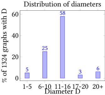
(a) Distribution of diameters (89.5% $\leq 16$).

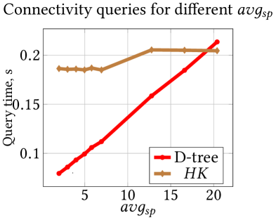
(b) D-tree outperforms $HK$ when $avg_{sp}\leq 16.6$.

Figure 10. Diameters for real-world graphs and $avg_{sp}$.

We quantify the difference between D-trees and $HK$ by comparing their connectivity query performance for different values of $avg_{sp}$, the average sum of lengths of the shortest paths over all pairs of vertices in a graph ($avg_{sp}$ is upper-bounded by the diameter). Let $C=(V^{\prime},E^{\prime})$ be a connected component and $dist_{C}(u,v)$ the length of the shortest path between $u\in V^{\prime}$ and $v\in V^{\prime}$,

$$avg_{sp}(C)=(\sum_{u<v}dist_{C}(u,v))/\binom{|V^{\prime}|}{2}.$$

As $avg_{sp}$ (and the diameter) is expensive to compute for a given graph, we generated synthetic graphs with a central node and $N=480$ other nodes arranged around this node. We connect $k$ line graphs, each containing $\nicefrac{{N}}{{k}}$ vertices, to the central node: this regular structure allows us to compute $avg_{sp}$ (and the diameter) more efficiently. Figure 10(b) shows the connectivity query performance of D-trees and $HK$ for different values of $avg_{sp}$. D-trees outperform $HK$ for graphs with $avg_{sp}\leq 16.6$, so we expect D-trees to outperform $HK$ for at least 89.5% of the real-world graphs from Figure 10(a), due to the diameter being an upper bound for $avg_{sp}$.

7.5. Comparison with BFS/DFS

We compared the runtime of connectivity queries for D-trees with that of BFS/DFS, which acts as a baseline. The worst-case runtime complexity of BFS/DFS is $O(|V|+|E|)$(Cormen et al., 2009) and our experiments confirm that the runtime of this approach is too high for practical purposes: on average, BFS/DFS is several orders of magnitude slower than D-trees. For example, for one of the smaller graphs, WI, running connectivity queries for all pairs of vertices, which amounts to around 25 million queries, takes BFS/DFS more than eight days to complete. In contrast, D-trees run this set of queries in 23 seconds. We ran the queries on the complete graph, i.e., we inserted all the edges without deleting any. Clearly, BFS/DFS does not have any maintenance costs, but it only took us 200ms to build the D-trees for the WI-graph from scratch.

7.6. Insertion-only Algorithms

Next, we compare D-trees with DBL and union-find (Tarjan, 1975, 1983), which is still considered the state-of-the-art algorithm for insertion-only graphs (Wulff-Nilsen, 2013). We measured the average query and insertion performance per operator for D-trees, DBL, and union-find on the large graphs (excluding SC, as DBL took too long to construct the 2-hop labeling). The left-hand side of Figure 11 shows the time for inserting all the edges. Clearly, DBL is the slowest algorithm (even though we ran the insertions in a batch, which adds the smallest overhead) and D-trees are slightly slower than union-find. The right-hand side of Figure 11 shows the average runtime of running 50 million random connectivity queries (after inserting all the edges in a first step). Unsurprisingly, union-find is the fastest algorithm, followed by D-trees, and DBL comes in last again. DBL is slow, because it needs to run BFS for the insertions and from time to time also for queries. Although, union-find is the fastest algorithm, it is not applicable to fully dynamic graphs. It does not support deletions, as it only maintains compressed paths from nodes to roots and does not preserve connections among non-root vertices.

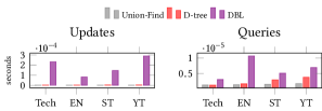
Figure 11. Average run time for insertions and queries.

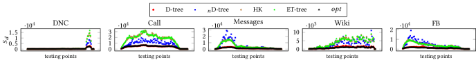
Figure 12. $S_{d}$ for spanning trees (forest) for graphs.

Figure 13. Query performance

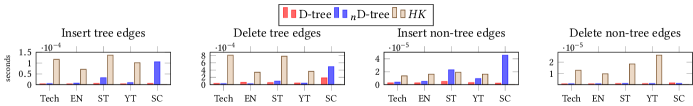
Figure 14. Average run time for updates.

7.7. Distances between Roots and Nodes

Here we confirm that the techniques we use for maintaining spanning trees, namely preserving BFS-trees (if possible to do so efficiently), considering short-cuts when inserting non-tree edges, and re-establishing the centroid property, lead to small values for $S_{d}$. In Figure 12, we show the value of $S_{d}$ for the current spanning forest for every snapshot. The upper row depicts the results for small graphs, for which we include the expensive methods $opt$ and ET-tree. The best possible spanning forest is created by $opt$, which computes the optimal BFS-tree. We observe that our D-tree is very close to $opt$ and much better than _nDtree, demonstrating the effectiveness of the heuristics for maintaining the spanning forest. Our D-tree also has better values for $S_{d}$ than the ET-tree and $HK$. The difference between the ET-tree and $HK$ is minimal since both employ a treap (Seidel and Aragon, 1996) to balance the tree. The lower row of Figure 12 shows the results for large graphs and, again, our D-tree creates trees with small $S_{d}$ values and is able to maintain the lead over time. We do not show results for $opt$ and ET-trees for large graphs, as these methods are very inefficient: $opt$ spends about 10 seconds per update on the ST-graph (in contrast to less than one millisecond for D-trees) and we do around 20 million updates in total per experiment; after a couple of updates on the ST-graph, deletions on ET-trees are three orders of magnitude slower than those on D-trees. We do not show results for $HK$ on the SC graph because $HK$ ran for fourteen days and was not able to finish in that time.

Figure 16 in the appendix gives a detailed insight into the distribution of node depths in the various trees. On average, the nodes in our D-trees are much closer to the roots. For small graphs (upper row of Figure 16), we are very close to $opt$. For large graphs (lower row of Figure 16), D-trees also outperform the other methods.

7.8. Performance for Connectivity Queries

As we have shown in Theorem 5.4, the average query costs are directly related to $S_{d}$. This is confirmed by our experiments on query performance in Figure 13. The results are strongly correlated to those for $S_{d}$ in Figure 12. The average Pearson correlation between $S_{d}$ and query time over all datasets is 0.904842. The upper row of Figure 13 for small graphs demonstrates that the performance of D-trees is very close to that of $opt$. Additionally, D-trees consistently outperform _nD-trees, ET-trees, and $HK$ for all graphs. $avg_{d}$, the average distances between nodes and roots, is less than ten in D-trees while $avg_{d}$ for $HK$ is several times larger.

7.9. Performance for Update Operations

Figure 14 shows the run times for update operations. First, we see that $HK$ is much slower than the other techniques (the differences are usually an order of magnitude). While balanced binary trees offer good worst-case performance, they are much deeper than D-trees. Moreover, $HK$ does not use spanning trees but a more complex representation, adding to the overhead of update operations. Next, we compare D-trees to _nD-trees to show the effectiveness and costs of our heuristics. When deleting non-tree edges, the differences are minimal: the overhead for preserving BFS-trees in D-trees is very small. We observe the biggest differences for inserting (tree and non-tree) edges. Since _nD-trees do not utilize any heuristics for minimizing $S_{d}$, the distances between the roots and other nodes in the spanning trees tend to grow over time. This has a negative impact on insertions (and not just queries), because we have to navigate to the roots of the spanning trees to determine whether we insert a tree or non-tree edge. When deleting tree edges, there is no clear winner between D-trees and _nD-trees. While D-trees have a smaller cut number, they search through all potential replacement edges to pick the best one (lowering $S_{d}$). _nD-trees terminate the search for a replacement edge as soon as they find the first one.

7.10. Discussion

D-trees outperform HK in querying and inserting tree and non-tree edges, because of the smaller $S_{d}$ in the D-trees. The ET-trees employed by HK are shaped differently and do not represent spanning trees directly. Basically, the occurrences of nodes in an Euler tour of a spanning tree are mapped into a balanced binary tree such that the in-order traversal of this tree is the Euler tour. This makes it independent of the diameter of a graph and results in trees of depth $\log_{2}(n)$ ($n$ being the number of nodes). Consequently, in the worst case, a lookup on this tree is still logarithmic in the number of nodes. However, it cannot take advantage of graphs with small diameters, the nodes are embedded much deeper in the tree compared to a D-tree. It gets even worse when deleting a non-tree edge: HK has logarithmic runtime for this case (in contrast to the constant runtime in D-trees). On average, D-trees have very small cut numbers $S_{c}$, usually less than fifteen, often smaller than ten. Due to the structure of the ET-tree, the splits are more even, resulting in longer searches on larger trees (usually more than an order of magnitude larger compared to D-trees). Even though D-trees go through all non-tree edges when searching for a replacement edge (while HK takes the first valid edge it finds), due to the small $S_{c}$ and $S_{d}$, this is still efficient.

8. Conclusion

We identify two crucial parameters for optimizing connectivity queries via spanning trees in fully dynamic graphs: $S_{d}$, the sum of distances between nodes in a tree and its root, and $S_{c}$, the cut number of a tree. Due to the high cost of maintaining trees that minimize $S_{d}$ and $S_{c}$, we develop a data structure, called D-tree with heuristics to keep the values of $S_{d}$ and $S_{c}$ small when updating the trees. This makes the evaluation of connectivity queries and the maintenance of spanning trees more efficient. Moreover, we show that it is possible to implement our heuristics with a low overhead, i.e., we only need to know the size of each subtree in a spanning tree. Extensive experiments with real-world datasets demonstrate that our approach has a performance close to optimal BFS-trees and outperforms algorithms that guarantee worst-case complexity. For instance, maintaining D-trees is up to fifty times faster than $HK$ and D-trees have a much better average query performance.

For future work, we plan to extend our approach for connectivity queries on (sparse) graphs with large diameters, such as road networks, by representing a connected component with multiple spanning trees to flatten them. We also want to make our approach workload-aware, i.e., adapt it to a given ratio of queries and update operations. Since our update operations are very efficient, we can afford to add some overhead in the form of further optimizations when faced with a high proportion of queries. Additionally, in the context of workload-awareness we want to consider the distribution of connectivity queries. We also plan to investigate if our approach can be adapted to directed graphs.

9. Appendix

Appendix A Examples

A.1. BFS tree

Example A.1.

In Figure 15, spanning trees $T_{3}$ and $T_{4}$ are BFS trees with root $n_{1}$ and $n_{2}$, respectively.

(a) $T_{3}$

(b) $T_{4}$

(c) $T_{5}$

Figure 15. Different spanning trees for $C_{1}$ in Figure 1. The red nodes are the roots of the spanning trees. $T_{1}$ in Figure 2, $T_{3}$ and $T_{4}$ are BFS trees for $C_{1}$. $T_{5}$ is not a BFS tree for $C_{1}$.

Appendix B Algorithms

B.1. Link

Algorithm 6 shows the pseudocode of link operation.

1

input : a node $n_{u}$ in D-tree $D$ with the root $r_{u}$, the root $n_{v}$ of a D-tree currently not connected to $D$ via a tree edge

output : merged D-tree with new tree edge ($n_{u},n_{v}$)

2

3add $n_{v}$ to $n_{u}.children$

4 $n_{v}.parent=n_{u}$

5

$m=Null$

 // new centroid

6 $i=n_{u}$

7 while $i\neq Null$ do

8      

9      $i.size=i.size+n_{v}.size$

10       if $i.size$¿ $\nicefrac{{(r_{u}.size+n_{v}.size)}}{{2}}$ and $m==Null$  then  $m=i$

11      

12      $i=i.parent$

13      

14

15if $m\neq Null$ and $m\neq r_{u}$ then  $r_{u}$ = reroot($m$)

16 return $r_{u}$

Algorithm 6 link($n_{u}$, $r_{u}$, $n_{v}$)

B.2. Unlink

Algorithm 7 shows the pseudocode of unlink operation.

1

input : a non-root node $n_{v}$ in D-tree $D$

output : two D-trees, not connected via tree edges

2

3$i=n_{v}$

4 while $i.parent\neq Null$ do

5       $i=i.parent$

6       $i.size=i.size-n_{v}.size$

7remove $n_{v}$ from $n_{v}.parent.children$

8 $n_{v}.parent=Null$

return ($n_{v}$, $i$)

Algorithm 7 unlink($n_{v}$)

B.3. Delete non-tree edge

Algorithm 8 shows the pseudocode for the deletion of a non-tree edge.

1

input : Tree nodes $n_{u}$ and $n_{v}$

output : Updated nodes $n_{u}$ and $n_{v}$

2

3remove $n_{u}$ from $n_{v}.nte$

4 remove $n_{v}$ from $n_{u}.nte$

Algorithm 8 delete_nte($n_{u}$, $n_{v}$)

Appendix C Proofs

C.1. Proof for Theorem 5.4

Proof.

When answering connectivity queries $conn(u,v)$, we traverse from $u$ and $v$ to the roots $r_{u}$ and $r_{v}$ containing them ($r_{u}$ and $r_{v}$ can be equal). Let $d_{R}(u)=d_{T}(r_{u},u)$ be the distance between a node and the root of its spanning tree. The cost of the traversal from node to root is directly proportional to $d_{R}(u)$. Consequently, the total cost $c_{tot}$ of connectivity queries over all pairs of nodes $u$ and $v$ ($u\neq v$) is equal to $\sum_{u<v}(d_{R}(u)+d_{R}(v))$

$$=\frac{1}{2}\left(\sum_{u\in V}\sum_{v\in V}(d_{R}(u)+d_{R}(v))-\sum_{u=v\in V}(d_{R}(u)+d_{R}(v))\right)$$

$$=\frac{1}{2}\left(\sum_{u\in V}\sum_{v\in V}(d_{R}(u)+d_{R}(v))\right)-\frac{1}{2}\cdot 2\sum_{u\in V}d_{R}(u)$$

$$=\frac{1}{2}\left(\sum_{u\in V}\sum_{v\in V}d_{R}(u)+\sum_{u\in V}\sum_{v\in V}d_{R}(v)\right)-\sum_{u\in V}d_{R}(u)$$

$$=\frac{1}{2}\left(|V|\sum_{u\in V}d_{R}(u)+|V|\sum_{v\in V}d_{R}(v)\right)-\sum_{u\in V}d_{R}(u)$$

$$=|V|\sum_{u\in V}d_{R}(u)-\sum_{u\in V}d_{R}(u)=(|V|-1)\sum_{u\in V}d_{R}(u)$$

So, the average cost $c_{\mbox{\scriptsize{\emph{avg}}}}$ per query (assuming uniformly distributed queries) is equal to

$$\frac{\sum_{u<v}(d_{R}(u)+d_{R}(v))}{\binom{|V|}{2}}=\frac{(|V|-1)\sum_{u\in V}d_{R}(u)}{\frac{|V|(|V|-1)}{2}}=$$

$$\frac{2\sum_{u\in V}d_{R}(u)}{|V|}=2E(d_{R}(u))$$

∎

C.2. Proof for Lemma 5.7

Proof.

Let us assume that we have a BFS-tree $T$ with root $r$ in which the sum of distances between $r$ and all other nodes is not minimal. Thus, there is at least one node for which we can find a shorter path to the root: we call this node $u$. The current path from $r$ to $u$ in $T$ is $r,u_{1}^{c},u_{2}^{c},\dots,u_{k}^{c},u$, while the shortest path is $r,u_{1}^{s},u_{2}^{s},\dots,u_{l}^{s},u$ with $k>l$. This is a contradiction to the definition of a BFS-tree. As a BFS-tree expands level by level, the node $u$ would have already been reached after $l$ steps via the path containing the nodes $u_{i}^{s}$. ∎

C.3. Proof for Lemma 5.13

Proof.

Let $D$ be the maximal depth of $T$ and $V_{d}=\{v|v\in V^{\prime},d_{T}(r,v)=d\}$ the vertices in $T$ with depth $d$. By Definition 5.1,

$$S_{d}(T) =\sum_{v\in V^{\prime}}d_{T}(r,v)$$

$$=\sum_{d=1}^{D}d*|V_{d}|$$

$$=|V_{1}|+2*|V_{2}|+3*|V_{3}|+...+D*|V_{D}|$$

$$=|V_{1}|+|V_{2}|+|V_{3}|+...+|V_{D}|$$

$$+|V_{2}|+|V_{3}|+...+|V_{D}|$$

$$+|V_{3}|+...+|V_{D}|$$

$$\dots$$

$$+|V_{D-1}|+|V_{D}|$$

$$+|V_{D}|$$

$$=\sum_{v\in V_{1}}size(v)+\sum_{v\in V_{2}}size(v)+\dots+\sum_{v\in V_{D}}size(v)$$

$$=\sum_{d=1}^{D}\sum_{v\in V_{d}}size(v)=\sum_{v\in V^{\prime}\setminus r}size(v)=S_{c}(T)$$

∎

C.4. Proof for Lemma 5.14

Proof.

According to Lemma 5.7, there is no other tree rooted at $r$ with a smaller value for $S_{d}$. Assume that $r$ is not a centroid of $T_{m}$. Let $c_{1},c_{2},\dots,c_{k}$ be the children of $r$. Since $r$ is not a centroid, one of the children of $r$, $c_{j}$, has a size greater than $\nicefrac{{|V_{m}|}}{{2}}$ (see Theorem 5.12). We designate $c_{j}$ as the new root of $T_{m}$, by making $r$ a child of $c_{j}$, creating the tree $T_{c_{j}}$. This pulls up $c_{j}$ and all its descendants by one level, while pushing down $r$ and all its other children ($c_{i}\not=c_{j}$) by one level:

$$S_{d}(T_{c_{j}}) =S_{d}(T_{m})-size(c_{j})+1+\sum_{i\not=j}size(c_{i})$$

$$=S_{d}(T_{m})-size(c_{j})+(size(r)-size(c_{j}))$$

$$=S_{d}(T_{m})+size(r)-2\cdot size(c_{j})<S_{d}(T_{m})$$

This contradicts that $S_{d}(T_{m})$ is minimal. ∎

Appendix D Experiments

D.1. Distributions of distances between nodes and roots

Figure 16 gives a more detailed insight into the distribution of node depths in the various trees. We accumulate the frequency of each node depth in spanning tress at all testing points, and calculate the average frequency of each node depth. On average, the nodes in our D-trees are much closer to the roots. For small graphs (upper row of Figure 16), we are very close to opt. For large graphs (lower row of Figure 16), D-trees also outperform the other methods.

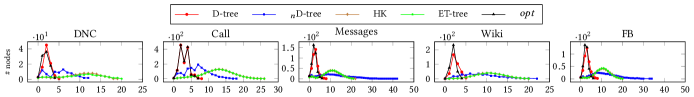
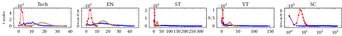
Figure 16. Distributions of average node depths.

D.2. Numbers of vertices and edges in graphs at each snapshot

Figure 17 and Figure 18 show the numbers of vertices and edges at each snapshot of the graphs respectively. In general, between two neighboring snapshots, more (fewer) insertions of edges than deletions of edges increases (decreases) the numbers of vertices and edges in the graphs.

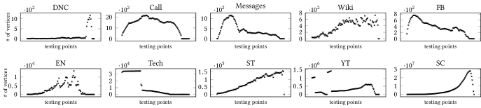
Figure 17. # vertices in graphs.

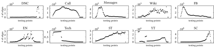
Figure 18. # edges in graphs.

D.3. Average distance between all nodes and roots in spanning trees

The average distance between all nodes and the root in the spanning tree is equal to $\frac{S_{d}}{|V|}$ where $|V|$ is the number of nodes in the spanning tree. Figure 19 shows the average distance between all nodes and roots in the spanning trees for large graphs at each snapshot. Such average distances in D-trees are the smallest (all less than 10) and the most stable at each testing point in all large graphs.

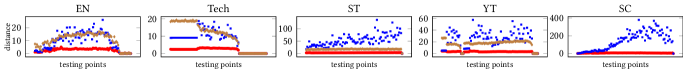
Figure 19. Average distance between nodes and roots in spanning trees (forests) for large graphs

D.4. Average cut number in spanning trees (forests) for graphs at each snapshot

The average cut number in the spanning tree is equal to $\frac{S_{c}}{|V|}$ where $|V|$ is the number of nodes in the spanning tree. Figure 20 shows the average cut numbers in the spanning trees for large graphs at each snapshot. Average cut numbers in D-trees are the smallest (all less than 15, in most cases less than 10) at each snapshot in all large graphs.

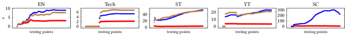
Figure 20. Average cut numbers for spanning trees (forests) for large graphs

D.5. Performances of update operations at each snapshot

Figure 21 shows performances of update operations between current snapshot and previous snapshot. Updates on larger graphs take more time than on smaller graphs. Overall, D-tree has the best update performances.

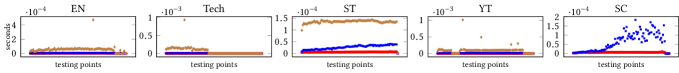
(a) Average run time of inserting tree edges

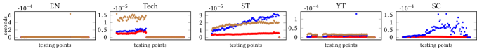
(b) Average run time of inserting non-tree edges

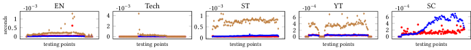
(c) Average run time of deleting tree edges

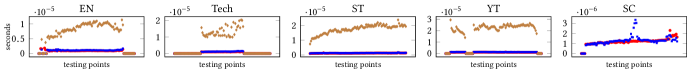
(d) Average run time of deleting non-tree edges

Figure 21. Average run time of update operations between current snapshot and previous snapshot in forest trees (forests) for large graphs.

References

- (1)
- dat (2021) 2021. SNAP: Stack Overflow temporal network. Retrieved October 21, 2021 from http://snap.stanford.edu/data/sx-stackoverflow.html
- KON (2022) 2022. KONECT: The KONECT Project. Retrieved June 02, 2022 from http://konect.cc/statistics/diam/
- Alberts et al. (1997) David Alberts, Giuseppe Cattaneo, and Giuseppe F. Italiano. 1997. An Empirical Study of Dynamic Graph Algorithms. ACM J. Exp. Algorithmics 2 (Jan. 1997), 5–es. https://doi.org/10.1145/264216.264223
- Ammar et al. (2018) Waleed Ammar, Dirk Groeneveld, Chandra Bhagavatula, Iz Beltagy, Miles Crawford, Doug Downey, Jason Dunkelberger, Ahmed Elgohary, Sergey Feldman, Vu Ha, Rodney Kinney, Sebastian Kohlmeier, Kyle Lo, Tyler Murray, Hsu-Han Ooi, Matthew Peters, Joanna Power, Sam Skjonsberg, Lucy Lu Wang, Chris Wilhelm, Zheng Yuan, Madeleine van Zuylen, and Oren Etzioni. 2018. Construction of the Literature Graph in Semantic Scholar. In NAACL. https://www.semanticscholar.org/paper/09e3cf5704bcb16e6657f6ceed70e93373a54618
- Bramandia et al. (2009) Ramadhana Bramandia, Byron Choi, and Wee Keong Ng. 2009. Incremental maintenance of 2-hop labeling of large graphs. IEEE Transactions on Knowledge and Data Engineering 22, 5 (2009), 682–698.
- Cheng et al. (2013) James Cheng, Silu Huang, Huanhuan Wu, and Ada Wai-Chee Fu. 2013. TF-Label: A Topological-Folding Labeling Scheme for Reachability Querying in a Large Graph (SIGMOD ’13). Association for Computing Machinery, New York, NY, USA, 12. https://doi.org/10.1145/2463676.2465286
- Chin and Houck (1978) Francis Chin and David Houck. 1978. Algorithms for updating minimal spanning trees. J. Comput. System Sci. 16, 3 (1978), 333–344. https://doi.org/10.1016/0022-0000(78)90022-3
- Cohen et al. (2002) Edith Cohen, Eran Halperin, Haim Kaplan, and Uri Zwick. 2002. Reachability and Distance Queries via 2-Hop Labels. In Proceedings of the Thirteenth Annual ACM-SIAM Symposium on Discrete Algorithms (San Francisco, California) (SODA ’02). SIAM, USA, 937–946.
- Cormen et al. (2009) Thomas H Cormen, Charles E Leiserson, Ronald L Rivest, and Clifford Stein. 2009. Introduction to algorithms. MIT press.
- Dobrynin et al. (2001) Andrey A Dobrynin, Roger Entringer, and Ivan Gutman. 2001. Wiener index of trees: theory and applications. Acta Applicandae Mathematica 66, 3 (2001), 211–249.
- Doraiswamy and Natarajan (2009) Harish Doraiswamy and Vijay Natarajan. 2009. Efficient algorithms for computing Reeb graphs. Computational Geometry 42, 6-7 (2009), 606–616.
- Eppstein (1992) D. Eppstein. 1992. Sparsification-a technique for speeding up dynamic graph algorithms. In Proc. of 33rd Annual Symposium on Foundations of Computer Science (FOCS’92). 60–69. https://doi.org/10.1109/SFCS.1992.267818
- Eppstein et al. (1997) David Eppstein, Zvi Galil, Giuseppe F. Italiano, and Amnon Nissenzweig. 1997. Sparsification—a Technique for Speeding up Dynamic Graph Algorithms. J. ACM 44, 5 (Sept. 1997), 669–696. https://doi.org/10.1145/265910.265914
- Eyal and Halperin (2005) Eran Eyal and Dan Halperin. 2005. Improved maintenance of molecular surfaces using dynamic graph connectivity. In International Workshop on Algorithms in Bioinformatics. Springer, 401–413.
- Frederickson (1983) Greg N. Frederickson. 1983. Data Structures for On-Line Updating of Minimum Spanning Trees. In Proc. of the 15th Annual ACM Symposium on Theory of Computing (STOC’83). Association for Computing Machinery, New York, NY, USA, 252–257. https://doi.org/10.1145/800061.808754
- Gibbons (1985) Alan Gibbons. 1985. Algorithmic graph theory. Cambridge university press.
- Hegeman and Iosup (2018) Tim Hegeman and Alexandru Iosup. 2018. Survey of Graph Analysis Applications. CoRR abs/1807.00382 (2018). arXiv:1807.00382 http://arxiv.org/abs/1807.00382
- Helmer et al. (2003) Sven Helmer, Thomas Neumann, and Guido Moerkotte. 2003. A Robust Scheme for Multilevel Extendible Hashing. In Proc. 18th Int. Sym. on Computer and Information Sciences (ISCIS). Antalya, Turkey, 220–227.
- Henzinger and King (1995) Monika Rauch Henzinger and Valerie King. 1995. Randomized dynamic graph algorithms with polylogarithmic time per operation. In Proc. of the 27th annual ACM symposium on Theory of computing (STOC’95). 519–527.
- Henzinger and King (1997) Monika Rauch Henzinger and Valerie King. 1997. Maintaining Minimum Spanning Trees in Dynamic Graphs. In Proc. of 24th Int. Colloquium on Automata, Languages and Programming (ICALP’97). Bologna, Italy, 594–604. https://doi.org/10.1007/3-540-63165-8_214
- Henzinger and King (1999) Monika Rauch Henzinger and Valerie King. 1999. Randomized Fully Dynamic Graph Algorithms with Polylogarithmic Time per Operation. J. ACM 46, 4 (1999), 502–516. https://doi.org/10.1145/320211.320215
- Henzinger and King (2001) Monika Rauch Henzinger and Valerie King. 2001. Maintaining Minimum Spanning Forests in Dynamic Graphs. SIAM J. Comput. 31, 2 (2001), 364–374. https://doi.org/10.1137/S0097539797327209
- Henzinger et al. (1999) Monika Rauch Henzinger, Valerie King, and Tandy Warnow. 1999. Constructing a tree from homeomorphic subtrees, with applications to computational evolutionary biology. Algorithmica 24, 1 (1999), 1–13.
- Holm et al. (2001) Jacob Holm, Kristian de Lichtenberg, and Mikkel Thorup. 2001. Poly-Logarithmic Deterministic Fully-Dynamic Algorithms for Connectivity, Minimum Spanning Tree, 2-Edge, and Biconnectivity. J. ACM 48, 4 (July 2001), 723–760. https://doi.org/10.1145/502090.502095
- Hopcroft and Tarjan (1973) John Hopcroft and Robert Tarjan. 1973. Algorithm 447: Efficient Algorithms for Graph Manipulation. Commun. ACM 16, 6 (June 1973), 372–378. https://doi.org/10.1145/362248.362272
- Huang et al. (2017) Shang-En Huang, Dawei Huang, Tsvi Kopelowitz, and Seth Pettie. 2017. Fully dynamic connectivity in O (log n (log log n) 2) amortized expected time. In Proceedings of the twenty-eighth Annual ACM-SIAM Symposium on Discrete Algorithms. SIAM, 510–520.
- Iyer et al. (2002) Raj Iyer, David Karger, Hariharan Rahul, and Mikkel Thorup. 2002. An Experimental Study of Polylogarithmic, Fully Dynamic, Connectivity Algorithms. ACM J. Exp. Algorithmics 6 (Dec. 2002), 4–es. https://doi.org/10.1145/945394.945398
- Jin et al. (2009) Ruoming Jin, Yang Xiang, Ning Ruan, and David Fuhry. 2009. 3-HOP: A High-Compression Indexing Scheme for Reachability Query. In Proceedings of the 2009 ACM SIGMOD International Conference on Management of Data (Providence, Rhode Island, USA) (SIGMOD ’09). Association for Computing Machinery, New York, NY, USA, 813–826. https://doi.org/10.1145/1559845.1559930
- Jordan (1869) Camille Jordan. 1869. Sur les assemblages de lignes. Journal für die reine und angewandte Mathematik 1869, 70 (1869), 185–190. https://doi.org/doi:10.1515/crll.1869.70.185
- Kapron et al. (2013) Bruce M. Kapron, Valerie King, and Ben Mountjoy. 2013. Dynamic graph connectivity in polylogarithmic worst case time. In Proc. of the 24th Annual ACM-SIAM Symposium on Discrete Algorithms, SODA’13. New Orleans, Louisiana, 1131–1142. https://doi.org/10.1137/1.9781611973105.81
- Kejlberg-Rasmussen et al. (2016) Casper Kejlberg-Rasmussen, Tsvi Kopelowitz, Seth Pettie, and Mikkel Thorup. 2016. Faster Worst Case Deterministic Dynamic Connectivity. In 24th Annual European Symposium on Algorithms (ESA’16), Piotr Sankowski and Christos D. Zaroliagis (Eds.). Aarhus, Denmark, 53:1–53:15. https://doi.org/10.4230/LIPIcs.ESA.2016.53
- Lyu et al. (2021) Qiuyi Lyu, Yuchen Li, Bingsheng He, and Bin Gong. 2021. DBL: Efficient Reachability Queries on Dynamic Graphs. In International Conference on Database Systems for Advanced Applications. Springer, 761–777.
- Mislove (2009) Alan Mislove. 2009. Online Social Networks: Measurement, Analysis, and Applications to Distributed Information Systems. Ph.D. Dissertation. Rice University, Department of Computer Science.
- Rossi and Ahmed (2015) Ryan A. Rossi and Nesreen K. Ahmed. 2015. The Network Data Repository with Interactive Graph Analytics and Visualization. In AAAI. http://networkrepository.com
- Sahu et al. (2017) Siddhartha Sahu, Amine Mhedhbi, Semih Salihoglu, Jimmy Lin, and M. Tamer Özsu. 2017. The Ubiquity of Large Graphs and Surprising Challenges of Graph Processing. Proc. VLDB Endow. 11, 4 (Dec. 2017), 420–431. https://doi.org/10.1145/3186728.3164139
- Sakr et al. (2021) Sherif Sakr, Angela Bonifati, Hannes Voigt, Alexandru Iosup, Khaled Ammar, Renzo Angles, Walid Aref, Marcelo Arenas, Maciej Besta, Peter A. Boncz, Khuzaima Daudjee, Emanuele Della Valle, Stefania Dumbrava, Olaf Hartig, Bernhard Haslhofer, Tim Hegeman, Jan Hidders, Katja Hose, Adriana Iamnitchi, Vasiliki Kalavri, Hugo Kapp, Wim Martens, M. Tamer Özsu, Eric Peukert, Stefan Plantikow, Mohamed Ragab, Matei R. Ripeanu, Semih Salihoglu, Christian Schulz, Petra Selmer, Juan F. Sequeda, Joshua Shinavier, Gábor Szárnyas, Riccardo Tommasini, Antonino Tumeo, Alexandru Uta, Ana Lucia Varbanescu, Hsiang-Yun Wu, Nikolay Yakovets, Da Yan, and Eiko Yoneki. 2021. The Future is Big Graphs: A Community View on Graph Processing Systems. Commun. ACM 64, 9 (Aug. 2021), 62–71. https://doi.org/10.1145/3434642
- Seidel and Aragon (1996) Raimund Seidel and Cecilia R Aragon. 1996. Randomized search trees. Algorithmica 16, 4 (1996), 464–497.
- Shiloach and Even (1981) Yossi Shiloach and Shimon Even. 1981. An On-Line Edge-Deletion Problem. J. ACM 28, 1 (Jan. 1981), 1–4. https://doi.org/10.1145/322234.322235
- Spira and Pan (1975) P.M. Spira and A. Pan. 1975. On Finding and Updating Spanning Trees and Shortest Paths. SIAM J. Comput. 4, 3 (1975), 375–380. https://doi.org/10.1137/0204032
- Szpankowski (1990) Wojciech Szpankowski. 1990. Patricia Tries Again Revisited. J. ACM 37, 4 (Oct. 1990), 691–711. https://doi.org/10.1145/96559.214080
- Tarjan (1975) Robert Endre Tarjan. 1975. Efficiency of a Good But Not Linear Set Union Algorithm. J. ACM 22, 2 (April 1975), 215–225. https://doi.org/10.1145/321879.321884
- Tarjan (1983) Robert Endre Tarjan. 1983. Data structures and network algorithms. SIAM.
- Tarjan and Vishkin (1984) Robert Endre Tarjan and Uzi Vishkin. 1984. Finding biconnected componemts and computing tree functions in logarithmic parallel time. In 25th Annual Symposium on Foundations of Computer Science, 1984. IEEE, 12–20.
- Tarjan and Vishkin (1985) Robert E Tarjan and Uzi Vishkin. 1985. An efficient parallel biconnectivity algorithm. SIAM J. Comput. 14, 4 (1985), 862–874.
- Thorup (2000) Mikkel Thorup. 2000. Near-Optimal Fully-Dynamic Graph Connectivity. In Proceedings of the Thirty-Second Annual ACM Symposium on Theory of Computing (Portland, Oregon, USA) (STOC ’00). Association for Computing Machinery, New York, NY, USA, 343–350. https://doi.org/10.1145/335305.335345
- Wei et al. (2018) Hao Wei, Jeffrey Xu Yu, Can Lu, and Ruoming Jin. 2018. Reachability Querying: An Independent Permutation Labeling Approach. The VLDB Journal 27, 1 (Feb. 2018), 1–26. https://doi.org/10.1007/s00778-017-0468-3
- West et al. (2001) Douglas Brent West et al. 2001. Introduction to graph theory. Vol. 2. Prentice hall Upper Saddle River.
- Wulff-Nilsen (2013) Christian Wulff-Nilsen. 2013. Faster deterministic fully-dynamic graph connectivity. In Proceedings of the twenty-fourth Annual ACM-SIAM Symposium on Discrete Algorithms. SIAM, 1757–1769.
- Zaroliagis (2002) Christos D. Zaroliagis. 2002. Implementations and Experimental Studies of Dynamic Graph Algorithms. Springer-Verlag, Berlin, Heidelberg, 2290–278.
- Zelinka (1968) Bohdan Zelinka. 1968. Medians and Peripherians of Trees. Archivum Mathematicum 4, 2 (1968), 87–95.
- Zhu et al. (2014) Andy Diwen Zhu, Wenqing Lin, Sibo Wang, and Xiaokui Xiao. 2014. Reachability Queries on Large Dynamic Graphs: A Total Order Approach. In Proceedings of the 2014 ACM SIGMOD International Conference on Management of Data (Snowbird, Utah, USA) (SIGMOD ’14). ACM, New York, NY, USA, 1323–1334. https://doi.org/10.1145/2588555.2612181