Multi-wavelength observations by XSM, Hinode and SDO of an active region. Chemical abundances and temperatures

Abstract

We have reviewed the first year of observations of the Solar X-ray Monitor (XSM) onboard Chandrayaan-2, and the available multi-wavelength observations to complement the XSM data, focusing on Solar Dynamics Observatory AIA and Hinode XRT, EIS observations. XSM has provided disk-integrated solar spectra in the 1–15 keV energy range, observing a large number of microflares. We present an analysis of multi-wavelength observations of AR 12759 during its disk crossing. We use a new radiometric calibration of EIS to find that the quiescent AR core emission during its disk crossing has a distribution of temperatures and chemical abundances that does not change significantly over time. An analysis of the XSM spectra confirms the EIS results, and shows that the low First Ionization Potential (FIP) elements are enhanced, compared to their photospheric values. The frequent microflares produced by the AR did not affect the abundances of the quiescent AR core. We also present an analysis of one of the flares it produced, SOL2020-04-09T09:32. The XSM analysis indicates isothermal temperatures reaching 6 MK. The lack of very high-T emission is confirmed by AIA. We find excellent agreement between the observed XSM spectrum and the one predicted using an AIA DEM analysis. In contrast, the XRT Al-Poly / Be-thin filter ratio gives lower temperatures for the quiescent and flaring phases. We show that this is due to the sensitivity of this ratio to low temperatures, as the XRT filter ratios predicted with a DEM analysis based on EIS and AIA gives values in good agreement with the observed ones.

1 Introduction

There is ample literature on observations and modelling of relatively large flares, of GOES X-class C and above, but comparatively little on the weaker flares in active region (AR) cores, despite the fact that they are much more frequent. We define here microflares as those events of GOES class A or below, not to be confused with larger flares, often also called microflares. The physics of microflares remains elusive, as key spectroscopic observations to study the evolution of 5–10 MK plasma have been lacking, as discussed in the review by Del Zanna et al. (2021). The review points out the need for high-resolution, high-sensitivity spectral imaging in the soft X-rays (100–150 Å) to study microflares.

An earlier statistical study based on GOES X-ray and Yohkoh Bragg Crystal Spectrometer (BCS) observations found a relationship between temperatures ($T_{\rm max}$) and X-ray emission measures (EM) at the peak of the X-ray emission, with lower-class microflares generally having lower temperatures (Feldman et al., 1996). A-class microflares had temperatures around 5 MK i.e. close to the ‘basal’ 2–3 MK values of active region cores (cf Del Zanna & Mason, 2018). One limitation of this and similar studies was the assumption that the plasma was isothermal.

Yohkoh Soft X-ray Telescope (SXT) broad-band observations of microflares in AR cores were used to obtain isothermal temperatures ranging between 4–8 MK (Shimizu, 1995), lasting for 2–7 min.

The sensitivity of the SphinX X-ray irradiance spectrometer, on board the CORONAS-PHOTON mission was higher than that of the earlier GOES X-ray monitors, and showed that microflares are indeed very common. Some studies of the general characteristcs of microflares, produced from the Bremsstrahlung emission and the isothermal assumption (see, e.g. Kirichenko & Bogachev, 2017), found a relation between $T_{\rm max}$ and EM for the smaller events that was different to that found by Feldman et al. (1996).

Studies of a few microflares, based on NuSTAR observations of the Bremsstrahlung emission and again the isothermal assumption (see, e.g. Hannah et al., 2019; Cooper et al., 2020; Duncan et al., 2021) have been published. Temperatures were in the range 4–8 MK and little evidence of non-thermal emission was generally found.

Several questions arise from previous studies of flares. First, is there a relation between the highest temperatures in the post-flare loops and the X-ray class ? The above-mentioned Feldman et al. (1996) study clearly indicates that larger flares have higher temperatures at their peak X-ray emission, but there are e.g. B-class flares that reach very different maximum temperatures. In the example discussed below, a B-class flare did not reach 7 MK, while in the textbook case of another B-class flare, observed by Hinode EIS (Culhane et al., 2007), a peak temperature of 12 MK was reached (Del Zanna et al., 2011). Perhaps such differences are related to the physical size of the flaring volume. A study of larger (GOES C8 class) flares by Bowen et al. (2013) indeed indicated that the peak temperature (in the 10–20 MK range) is inversely correlated with flare volume.

Second, is the isothermal assumption reasonable for small flares? To address this question, detailed spectroscopic observations are needed. Some information was obtained by Mitra-Kraev & Del Zanna (2019) with the analysis of Hinode EIS observations of a microflare. This event was composed of a bundle of strands being activated at similar times, with sizes that appeared resolved at the AIA resolution, 1″. The EIS spectra indicated that these strands had relatively low peak temperatures (about 4–5 MK) and were nearly isothermal in their cross-section, although the 5–10 MK temperature range was not well constrained (see also Winebarger et al., 2012, on the limitations in this range). The EIS results were consistent with the broad-band observations by the Solar Dynamics Observatory/Atmospheric Imaging Assembly (SDO/AIA) (Lemen et al., 2012) and Hinode XRT. Multi-wavelength observations of several other microflares were studied by Mitra-Kraev & Del Zanna (2019), indicating that the example provided was a ’typical’ case.

Another science questions about microflares relates to their possible contribution to the basal heating in AR cores. This basal emission has peak near-isothermal emission around 3 MK and does not significantly change its characteristics over time (Del Zanna, 2013a; Del Zanna et al., 2015). Detailed studies about the frequency of microflares have been lacking. They have typical lifetimes of about 10 minutes as seen in the EUV (Mitra-Kraev & Del Zanna, 2019). The older X-ray observations of AR cores from the Solar Maximum Mission (SMM) X-ray polychromator (Acton et al., 1980) Bent Crystal Spectrometer (BCS) also showed common weak flaring emission on those timescales (Del Zanna & Mason, 2014), so it is possible that they were the same type of events. The Mg xii images from CORONAS-PHOTON also show a peak in the distribution of AR flaring events around 10 minutes (Reva et al., 2018), although it is not clear if these are the same features (temperatures are uncertain as Mg xii can be formed between 5 and 25 MK).

Larger flares such as the B-class textbook case (Del Zanna et al., 2011) show quick chromospheric evaporation and filling of the flare loops with hot (above 10 MK) plasma, with a slow cooling phase where the plasma radiates at all temperatures whilst draining back to the chromosphere. In contrast, microflare loops are observed to cool down to nearly the background 3 MK, but then drain/disappear very quickly and do not show emission at lower temperatures (Mitra-Kraev & Del Zanna, 2019). This suggests that microflares do not contribute to the basal emission in AR cores.

The chemical abundances of the flaring plasma also hold key information related to the heating and cooling. The chemical abundances of low- FIP elements such as Fe, Si, relative to those of high-FIP ones such as S,O,Ne were found to be increased by a factor of about 3.2 (with respect to the photospheric values) for AR cores, regardless of their size and age (Del Zanna, 2013a; Del Zanna & Mason, 2014). This is the so-called FIP effect.

The FIP effect has gained a lot of interest in recent literature. It is most likely caused by ion-neutral separation in the chromosphere, due to the Ponderomotive force of trapped Alfven waves in magnetically-closed loops (see references in Laming, 2015). Observationally, there has been a wide range of different chemical abundances measured in coronal plasma, as reviewed by Laming (2015); Del Zanna & Mason (2018). Regarding large flares, there is ample evidence that the flare loops have near-photospheric abundances. We do not have measurements of abundances in microflares, but if they were available and were also photospheric, that would also provide an indication that microflares do not contribute to the basal emission in AR cores.

The Solar X-ray Monitor (XSM) (Vadawale et al., 2014; Shanmugam et al., 2020) onboard Chandrayaan-2 has been providing disk-integrated spectra in the 1 – 15 keV energy range since September 2019, providing temperatures, emission measures, and absolute chemical abundances of a few elements, with timescales of the order of a minute. XSM has a much greater sensitivity than previous GOES X-ray monitors, and is able to observe microflares down to A 0.01 class. A discussion of sub-A class flares during the minimum of solar cycle 24, and which occurred outside of ARs was presented in Vadawale et al. (2021a). The instrument has also been used to study the X-ray emission of the global quiet Sun corona, which was found to be dominated by X-ray bright points. A temperature close to 2 MK and a coronal FIP bias of about two were found (Vadawale et al., 2021b).

XSM does not have enough sensitivity to measure chemical abundances for individual microflares, but is able to do so for B-class flares. Mondal et al. (2021) presented a time-resolved spectroscopic analysis of several B-class flares occurring in AR cores. During the peak of the X-ray emission, temperatures reached 6–8 MK, whilst the chemical abundances of Mg, Al, and Si decreased towards their photospheric values. Similar decreases in the abundances were found at the peaks of larger flares by the Miniature X-Ray Solar Spectrometer (MinXSS) CubeSat (Woods et al., 2017; Moore et al., 2018). During the gradual decay phase, the XSM measurements found that the chemical abundances returned to their pre-flare coronal values. The MinXSS and XSM measurements are the first observations of this kind, providing new observational constraints to models of the atmosphere which include element fractionation, such as those of Laming (2017).

To complement the XSM observations, in particular to understand the spatial distribution of the X-ray emission observed by XSM, we have run several multi-wavelength campaigns, including Hinode HOP 396. For this paper, we have selected observations during March/April 2020, when a single AR (NOAA 12759) crossed the solar disk and produced many microflares and several B-class flares. The main aim of this paper is to present a multi-wavelength analysis of Hinode XRT and EIS observations, combined with XSM and SDO/AIA during the AR disk passage, to establish the active region core temperatures and abundances, and discuss the temperatures of one of the flares, as measurable by these instruments.

2 Observations and Data Analysis

We have analysed a large number of microflares observed by XSM during the first period of operations and searched for suitable Hinode observations. We have selected for presentation here observations of AR 12759 during its disk crossing, as a direct comparison between the XSM irradiances and the signal measured by the other instruments is straightforward, as this was the only AR on the disk. Also, we selected one of the flares to study, which occurred on Apr 9, as it had XRT coverage. EIS observed the AR in several instances during its quiescent phase, but did not observe any flares.

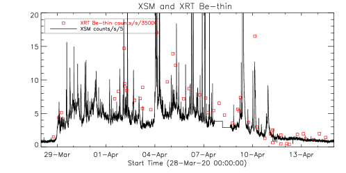
Figure 1: Top: the XSM 1–15 keV light curve (count rates averaged over 1 minute and scaled by a factor of 5) during the disk crossing of AR 12759. The red boxes indicate the scaled count rates from the full-disk Be-thin XRT filter. Bottom: the XSM light curves during three key periods selected for further analysis (see text).

2.1 XSM

XSM observes the Sun from a lunar orbit. It provides disk-integrated solar spectra at every second in the energy range of 1-15 keV with an unprecedented energy resolution of 180 eV at 5.9 keV (Mithun et al., 2020). The observed raw (level-1) spectra at every second are stored in a day-wise data file. Since the visibility of the Sun varies within the XSM field of view and the Sun also gets occulted by the moon, the level-1 data contains both solar spectra as well as non-solar background. We used XSM Data Analysis Software (Mithun et al., 2021) to generate the level-2 science data product for the Solar observations by selecting the Good Time Intervals (GTI) based on the observing geometry and a few other instrumental parameters. To do a spectral analysis of the XSM spectra we used the “chisoth” model  (Mondal et al., 2021). This is a local model of X-ray spectral fitting package (XSPEC) (Arnaud, 1996), meant for the spectral fitting of the observed X-ray spectrum. The “chisoth” model calculates the synthetic photon spectrum from a spectral library, generated by using CHIANTI v.10. The model takes the logarithm of the temperature, abundances of the elements with Z$=$2 to Z$=$30, and the volume emission measure as input parameters.

Fig. 1 shows the XSM 2–15 keV lightcurve during the disk crossing of AR 12759. By March 28 the outer part of the AR appeared outside the east limb, when the X-ray ‘background’ increased. During its disk crossing, this AR (the only one on the visible disc) produced many microflares. A few of the larger, B-class flares have already been analysed by Mondal et al. (2021). In all those cases, the behaviour of the chemical abundances was similar, i.e. the abundances were closer to photospheric values during peak X-ray emission. By April 12 the core of the AR was behind the west limb. This paper focuses on an analysis of the quiescent emission from the AR during its disk crossing on the Apr 1, 4, 8 and the B-class flare that peaked on Apr 9 around 9:12 UT. The XSM lightcurves for Apr 1, 4, 9 are shown in Fig. 1 (bottom plots, on Apr 8 XSM did not observe).

2.2 Hinode XRT

We processed the XRT images using the standard SolarSoft procedures, paying particular attention in removing saturated images and taking into account the pointing information stored in the XRT database (SolarSoft dbase). To obtain the temperatures, we used CHIANTI v.10 (Del Zanna et al., 2021) atomic data and calculated the responses. The Al poly / Be thin filter ratio is essentially insensitive to different chemical abundances .

We have analysed full-Sun XRT synoptic observations during the AR disk crossing. The averaged count rates in the Be-thin filter for a selection of dates are shown in Fig. 1 as boxes, scaled by a normalization factor. There is generally good agreement in the variability of the XRT signal in this filter and the XSM count rates, as expected. This is because the XSM sensitivity is close to that of this XRT filter. The XRT Be-thin full-disk images are also very useful for checking that AR 12759, even during quiescence, is dominating the full-disk signal. This means that the XSM signal is also dominated by the active region, making a direct comparison between XSM and the other instruments (XRT, EIS, AIA) possible.

There are also many XRT partial-frame observations of the active region during its disk crossing, with the same filters. We have used one set for a direct EIS/XRT cross-calibration.

For each XSM flare we searched for available XRT observations. As microflares last about 10 minutes, it was essential to obtain an XRT cadence of about a minute, which was obtained with a reduced FOV and the use of two filters. In many instances, the automatic exposure control (AEC), a safety measure for the instrument, was too slow to reduce the exposures, and the XRT images during the peak of the microflares were saturated (the standard AEC works relatively well for larger flares, as they have a longer duration). One observation which we could use for analysis was the flare on Apr 9, produced by AR 12759, where XRT used the Al-poly and Be-thin filters.

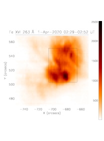
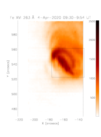
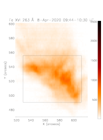
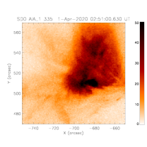
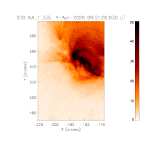
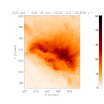
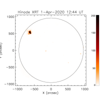
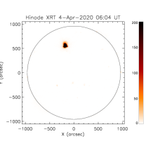
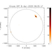
Figure 2: Top row: selected regions (boxes) of the AR 12759 core EIS observations during its disk crossing on 2020 Apr 1, 4, and 8. The images show the integrated radiances in the Hinode EIS Fe XVI 263 Å line, in calibrated units. Middle row: SDO AIA 335 Å images during the EIS observations, in DN/s. Bottom row: XRT Be-thin images (DN/s) at times close to the EIS observations. All images are negative.

2.3 Hinode EIS

For each XSM flare we searched for available EIS observations,but found none. However, there is an excellent set of observations of AR 12759 during its disk crossing, allowing us to check the active region evolution.

To process EIS data, we used custom-written software which mostly follows the standard SolarSoft programs, with the exception that the bias is subtracted while doing the line fitting, and the particle hits are removed by averaging procedures along the slit direction.

The main issue we faced in the analysis is related to the EIS radiometric calibration, and its variations in time and wavelength. Del Zanna (2013b) presented a significant revision of the ground calibration, with an additional time-dependent decrease in the sensitivty of the long-wavelength channel, however this was only valid until 2012, and indicated that further wavelength-dependent corrections with time would eventually be needed. A long-term programme was therefore started to analyse data after 2013 and provide a new radiometric calibration. The preliminary results of this study (Del Zanna and Warren, 2022, in prep) are used here. More details are provided in the Appendix.

2.4 SDO/AIA

As EIS did not observe the flare on April 9, we used SDO AIA data to study the thermal structure of the flare. We have used Mark Cheung’s Differential Emission Measure (DEM) code (Cheung et al., 2015). As input we used averaged images over 36 s (images at 3 consecutive times) from the six EUV AIA channels (94, 131, 171, 193, 211, 335 Å) to derive EM maps. We took a minimum log $T$ [K] = 5.7 and 13 temperature bins of width 0.1 dex. The SDO/AIA response functions were calculated using CHIANTI version 10 considering a constant pressure of 10¹⁵ cm^-3 K and chosen abundances. We used the effective areas with the estimated degradation in the various channels as available within SolarSoft, noting that such degradation was extrapolated from the last calibration sounding rocket flight which flew in 2018. Hence, some additional uncertainty is present.

3 Results

Figure 3: DEM for the AR core observed on 2020 Apr 1, obtained from Hinode EIS. The points are plotted at the temperature $T_{\rm max}$, and at the theoretical vs. the observed intensity ratio multiplied by the DEM value.

Table 1: List of emission lines from the 2020 Apr 1 active region core. $\lambda_{\rm obs}$ (Å) is the measured wavelength. DN is the number of total counts in the line, while $I_{\rm obs}$ is the calibrated radiance (phot cm^-2 s^-1 arc-second^-2) obtained with our new EIS calibration. $T_{\rm max}$ and $T_{\rm eff}$ are the maximum and effective temperature (log values in K), $R$ the ratio between the predicted and observed radiances, Ion and $\lambda_{\rm exp}$ (Å) the main contributing line, and $r$ the fractional contribution to the blend.

$\lambda_{\rm obs}$	DN	$I_{\rm obs}$	$T_{\rm max}$	$T_{\rm eff}$	$R$	Ion	$\lambda_{\rm exp}$	$r$
195.98	904	13.9	5.71	5.90	1.01	Fe viii	195.972	0.85
275.36	361	52.0	5.79	5.92	0.85	Si vii	275.361	0.99
280.73	62	17.4	5.79	5.93	0.75	Mg vii	280.742	0.91
188.49	1920	61.2	5.94	6.05	0.87	Fe ix	188.493	0.90
197.86	1580	29.1	5.96	6.07	0.86	Fe ix	197.854	0.88
184.54	2610	194.0	6.05	6.14	0.94	Fe x	184.537	0.94
192.81	6300	122.0	6.13	6.18	0.88	Fe xi	192.813	0.94
180.40	2330	856.0	6.13	6.19	1.09	Fe xi	180.401	0.97
271.98	1040	119.0	6.15	6.21	1.02	Si x	271.992	0.97
192.40	13700	283.0	6.20	6.22	1.10	Fe xii	192.394	0.96
264.23	830	97.2	6.18	6.24	0.73	S x	264.231	0.98
202.05	10300	579.0	6.25	6.27	0.81	Fe xiii	202.044	0.96
251.95	1500	379.0	6.25	6.27	1.00	Fe xiii	251.952	0.97
188.67	1200	36.7	6.21	6.27	0.87	S xi	188.675	0.58
						Fe xii	188.679	0.11
						Fe xi	188.630	0.13
281.41	102	30.4	6.26	6.30	0.90	S xi	281.402	0.84
						Fe xi	281.367	0.13
285.83	83	46.0	6.27	6.31	0.73	S xi	285.823	0.97
246.89	98	39.6	6.27	6.31	0.70	S xi	246.895	0.98
264.78	6230	726.0	6.29	6.33	0.98	Fe xiv	264.789	0.93
211.32	2660	913.0	6.30	6.33	1.07	Fe xiv	211.317	0.97
278.27	31	7.1	6.32	6.36	0.69	P xii	278.286	0.95
288.40	131	111.0	6.35	6.39	0.70	S xii	288.434	0.98
284.15	10700	4620.0	6.34	6.40	1.15	Fe xv	284.163	0.98
194.42	432	7.3	6.53	6.42	0.89	Ar xiv	194.401	0.75
						Fe xi	194.442	0.13
256.68	2440	398.0	6.42	6.44	0.74	S xiii	256.685	0.98
262.98	2200	263.0	6.43	6.44	1.00	Fe xvi	262.976	0.96
249.18	680	227.0	6.48	6.47	0.65	Ni xvii	249.186	0.96
193.88	1110	19.7	6.57	6.48	1.02	Ca xiv	193.866	0.96
201.00	200	7.3	6.64	6.48	1.07	Ca xv	200.972	0.84

3.1 EIS results for the quiescent AR core

Hinode EIS observed AR 12759 during its disk crossing with several studies. We analysed the ATLAS_60 spectra, obtained with 60 s exposures on Apr 1,4, and 8 to obtain the DEM and the FIP effect in the AR core. There was no significant variability in the AR core during these three observations, as seen in the XSM light curves (cf Fig. 1, bottom plots) and as observed from XRT. For each observation, we selected an AR core region using the intensity of the Fe XVI 263 Å line, as shown in Fig. 2. The figure also shows AIA 335 Å images, which are dominated in the AR core by Fe XVI, and full-Sun XRT Be-thin images, which show that the AR was dominating the signal from the Sun. The AIA full-disk images were used to coalign EIS. The AR on Apr 1 was close to the east limb, on the 4th it was close to meridian and on the 8th it was close to the west limb.

We adopted the Del Zanna (2013a) chemical abundances, where the FIP bias is 3.2 (low FIP elements increased compared to their photospheric abundances) and used CHIANTI v.10 to obtain DEMs. To calculate the line emissivities we used a constant electron density of 2$\times$10⁹ cm^-3, a typical average AR value which fits the main EIS density-sensitive line ratios. The DEM was obtained using the method described in Del Zanna (1999), where the $DEM$ is assumed to be a spline function, and considering only low-FIP ions.

The DEM for Apr 1st is shown in Fig. 3. Those for Apr 4, 8 are similar and are shown in the Appendix. The plasma distribution in temperature has two peaks, one around 1.5 MK, typical of the diffuse emission in the AR core, and one around 3 MK, typical of the nearly isothermal hot AR core loops. Both temperature structures have an FIP bias of about 3, as the main lines are well reproduced within 20–30% (the uncertainty in the radiometric calibration).

Table 3 lists a small selection of the lines, showing a relatively good agreement between the low FIP elements (e.g. Fe, Si, Ca) and the high-FIP element argon. There are several argon lines in the EIS spectra, but they are all extremely weak in AR core spectra and blended to some degree, some with unknown transitions. The strongest line is an Ar XIV at 194.4 Å, very close to a stronger unidentified line at 194.35 Å.

Note that sulphur has a FIP of 10 eV, but can be used as a proxy for the high-FIP elements. In fact, in remote-sensing observations its variations are in line with those of the high-FIP elements. The sulphur EIS lines are strong and cover a wide temperature range, as are the iron lines, so the Fe/S results are more accurate than Ar/Fe. A few weak lines from other elements (e.g. K, P, Al) are also present and confirm the chosen abundances.

The Table also gives the total counts (DN) in the lines, as well as the calibrated intensities. It also indicates $T_{\rm max}$, the temperature where the line contribution function $G(T)$ has a maximum, and the effective temperature $T_{\rm eff}$:

$$T_{\rm eff}=\int G{\left({T}\right)}~{}DEM{\left({T}\right)}~{}T~{}dT/{\int G{\left({T}\right)}~{}DEM{\left({T}\right)}~{}dT}\quad,$$ (1)

that is an average temperature more indicative of where a line is formed.

The DEM results of the AR core regions selected for Apr 4th and Apr 8th are similar, as shown in the Appendix, although the AR core on the 8th had a lower emission in the high temperature peak. We also find, importantly, that the chemical abundances of the quiescent AR core do not vary, regardless of the age and the fact that many flares occurred. This result agrees with our previous studies of several active regions.

3.2 XSM results for the quiescent AR core

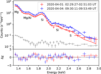
Figure 4: XSM spectrum during the quiescent phase of AR 12759 (red and blue points with error-bars), together with the best fit model spectrum (red and blue solid lines) and the background signal (grey). The lower panel shows the residuals between observations and best fit model.

Table 2: AR parameters obtained from the XSM spectrum. The abundances of Mg,Al, Si are in dex. The EIS abundances are the reference values of Del Zanna (2013a) adopted here. The Feldman are those listed by Feldman (1992), while the photospheric ones are from Asplund et al. (2009).

Date	log10(T)	EM	Mg	Al	Si
	(K)	(1046 cm-3)
01-04-2020	$6.47^{+0.01}_{-0.01}$	$8.67^{+1.9}_{-1.9}$	$7.78^{+0.07}_{-0.06}$	$7.05^{+0.11}_{-0.12}$	$7.89^{+0.05}_{-0.04}$
04-04-2020	$6.50^{+0.02}_{-0.01}$	$10.79^{+2.5}_{-1.7}$	$7.72^{+0.1}_{-0.08}$	$7.03^{+0.16}_{-0.17}$	$7.82^{+0.06}_{-0.06}$
EIS			(8.10)	6.95	8.00
Feldman			8.15	7.04	8.10
Phot.			7.6	6.45	7.51

To measure the absolute FIP effect in the AR core, we have analyzed the XSM spectra of the quiescent AR on April 1 from 02:29:27 UT to 02:51:03 UT, and April 4 from 09:30:11 UT to 09:53:49 UT, the timings of the EIS core observations. Due to the presence of the single AR on the solar disk, the XSM X-ray emission during this time was dominated by the AR core emission. We have fitted the XSM spectra with a single temperature model by considering the temperature, EM, and the abundances of Mg, Al and Si as a free parameters. Figure 4 shows the XSM best fit model spectra (red and blue solid lined) along with the observed ones (red and blue points). The best fitted parameters along with the 1-$\sigma$ error-bars are given in Table 2. The isothermal temperature of 3 MK agrees with the peak in the DEM as measured by Hinode EIS. The absolute abundances of Mg, Al and Si are given in dex. The silicon feature is the most prominent in the XSM spectra. The Si abundance is within 25% the Del Zanna (2013a) AR core values. The Al abundance is also close, while the Mg abundance as measured by XSM is lower. We note that the relative Al and Si abundances were measured by Del Zanna (2013a) using lines formed at lower temperatures, between 1 and 1.5 MK, while the Mg abundance was estimated by assuming the same increase over the photospheric value as Si (the Mg lines in the EIS spectra are formed at much lower temperatures). Del Zanna (2013a) estimated the absolute abundances assuming a unitary filling factor and measuring the path length of an AR core loop, so the agreement with the XSM result is remarkable.

3.3 XRT temperatures and EIS / XRT cross-calibration

We have analysed several XRT observations of the AR (at non-flaring times), and found consistently that the Be-thin/Al-Poly filter ratio has a value around 0.13 in the AR core. This value is equivalent to a temperature of about 2 MK, significantly lower than the 3 MK measured by XSM. Also, as shown below, the isothermal temperatures obtained from this XRT filter ratio are significantly lower than those measured by XSM during the B-class flare.

We initially thought that this discrepancy could be due to an XRT calibration issue. There have been several reports in the literature about a discrepancy between the estimated and measured XRT count rates (see, e.g. Mitra-Kraev & Del Zanna, 2019, and references therein), but not on possible problems in the relative calibration of the two channels.

We also know that a leakage of visible light in some of the filters can significantly affect some filter ratios (but not the Be-thin). Currently, it is possible to correct for this leakage by subtracting specially selected calibration images from full-frames, but not for partial frames. Also, the leakage can be more pronounced in partial frames. So, we first checked Al-Poly full-disk calibration data, which is essentially a flat field, and found that the variations between the center and the edges of the FOV are within a few DN/s, hence are negligible. Then we analysed several full-frame XRT synoptic datasets, and obtained isothermal temperatures for the AR core. The central part of the AR core is generally saturated in the synoptic observations (either in the Al-Poly or the Be-thin), except the 1s exposures, where the signal is often low, so combined images with different exposures need to be used. The full-disk filter ratios consistently indicate a temperature of 2 MK, i.e. the same as that obtained from the partial-frame filter ratios. We therefore conclude that leakage of visible light does not affect the partial frame Be-thin/Al-Poly observations of this active region.

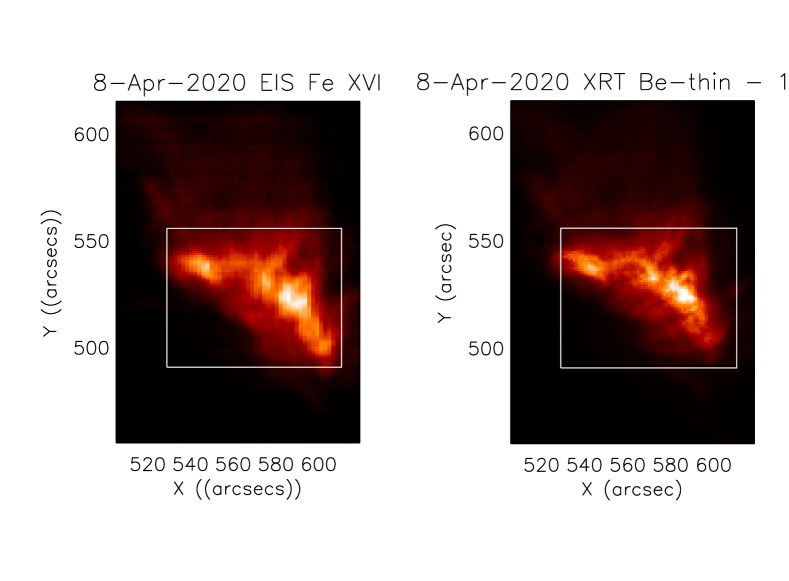
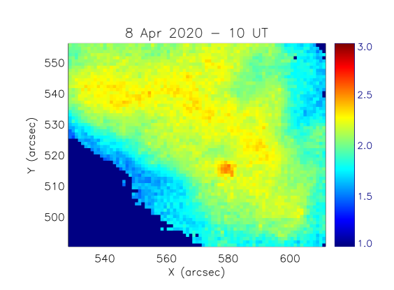
Figure 5: Top: the EIS raster image in Fe xvi and an XRT Be-thin image of the AR core. The selected box was used to obtain a DEM from EIS and averaged signal in the XRT filters. Bottom: isothermal temperature (MK) map in the box region, obtained from the Be-thin/Al-Poly filter ratio.

To investigate this issue further, we analysed the XRT observations on April 8 and performed a cross-calibration with EIS. A detailed pixel-by-pixel comparison is difficult, as the two instruments have different spatial and temporal resolutions, and as the EIS jitter is difficult to quantify. So we opted for an overall cross-calibration of the whole AR core. We co-aligned the XRT images against EIS/AIA. Three Be-thin averaged frames around 10 UT are shown in Fig. 5 (top). We then obtained from the Be-thin/Al-Poly filter ratio the isothermal temperature map in the AR core region (box), shown in Fig. 5 (bottom). The averaged temperature is 2 MK. The averaged XRT signal in the AR core in each of the two filters changed by only a few percent during the EIS observation. The averaged values are 31.6 DN/s in the Be-thin and 233.2 in the Al-Poly, resulting in a ratio of 0.136. The ratio varied between 0.133 and 0.139 during the EIS scan of the AR core.

As we have a relatively reliable EIS absolute calibration, we can predict the averaged AR core signal in the two XRT filters. The main issue here is the chemical abundance of the elements. Having confirmed from the EIS and XSM analysis that the Ar, S, Si, Fe abundances are consistent with the Del Zanna (2013a) abundances, indicating an FIP effect of 3.2, we have assumed that the abundances of the other elements contributing to the XRT bands (mainly O, Ne) follow the same trend, which is consistent to the X-ray results obtained by Del Zanna & Mason (2014).

We used the DEM obtained from EIS, which has two peaks, one around 1.8 MK and one around 2.5 MK, and calculated the XRT signal using the current knowledge of the XRT effective areas as available in SolarSoft. We obtained the simulated spectra shown in the Appendix and an averaged value of 25 DN/s in the Be-thin and 196 in the Al-Poly, resulting in a ratio of 0.128, i.e. only 6% lower than observed, and corresponding to an isothermal temperature of 2 MK. The absolute DN/s are also very close, within 26 and 19%, which is a remarkable result, considering the uncertainty in the calibration of the instruments and in the chemical abundances.

In conclusion, the lower isothermal temperatures obtained for the AR core by the XRT Be-thin/Al-Poly filter ratio are simply due to the fact that the Al-Poly is sensitive to low temperatures, so the isothermal temperature has a significant contribution from the peak in the emission measure around 1.8 MK.

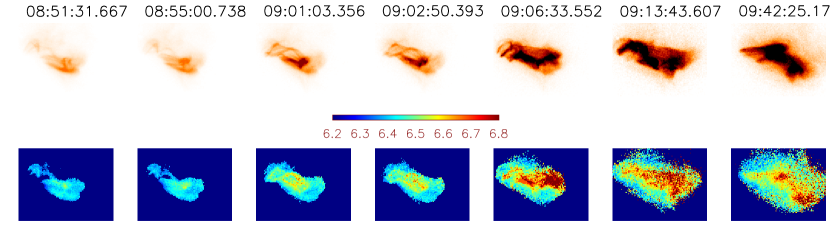
Figure 6: XRT negative images (top) and isothermal temperatures (bottom) for a selection of times during the B-class flare on 2020 Apr 9.

Figure 7: Isothermal temperatures obtained from XSM and XRT during the Apr 9 9:30 UT flare.

3.4 The 9:15 UT flare

The AR produced a B-class flare which started around 9:00 UT and finished by 9:50 UT. Fig. 6 shows a selection of XRT images and corresponding isothermal temperatures obtained from the Be-thin/Al-Poly filter ratio. The two filters had exposures within a few seconds, but several images were saturated and were discarded. The flare started with an activation of a filament and a compact X-ray emission. Later on, many flare loops became activated and occupied a significant fraction of the AR core, reaching peak X-ray intensity around 9:15 UT.

From the XRT filter ratio we have also obtained the emission measure for each pixel. We have then obtained averaged temperatures for the whole AR, weighted by the EM values, to be compared to the isothermal temperatures obtained from the spectral fitting of XSM. The XSM spectra were binned in time to increase the signal to noise. The results are shown in Fig. 7. XSM indicates a peak temperature of nearly 6 MK, while the peak temperature from XRT is much lower, although the variations are similar. We have verified that the X-ray signal from the AR is dominating over that from the whole Sun, looking at the full-Sun X-ray Be-thin images. Therefore, the XRT temperatures should be directly comparable to those of XSM.

We note that fitting the XSM spectra with a two temperature component (one for the quiescent AR core emission and one for the flare emission) would result in a slightly higher flare component, and the discrepancy would remain.

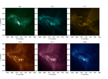
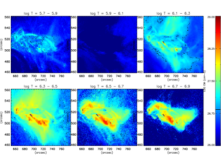
Figure 8: Top: SDO AIA EUV images at 9:12 UT, during the peak of the microflare. Bottom: DEM in selected temperature bins obtained from the images.

As the isothermal assumption is clearly an approximation for both the XSM and XRT datasets, we have explored the effects that a DEM distribution has for this flare. We selected a time close to the peak, at 9:12 UT, and obtained a DEM from the six AIA coronal images. We averaged the AIA data over a minute around 9:12 UT. Fig. 8 (top) shows the AIA EUV images. Hot emission is visible in the AIA 94 Å band, due to Fe xviii, as described in Del Zanna (2013a). Note that the filament is still visible in absorption at this wavelengths, but not in the XRT X-ray images. It is clear from inspection of the other AIA channels that this flare did not reach temperatures above 10 MK, otherwise the Fe xxi line would have contributed to the 131 Å band.

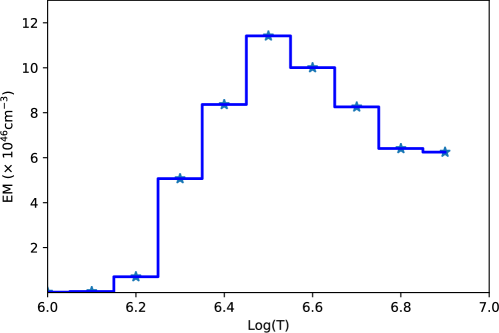
Figure 9: Averaged volume EM obtained from the AR core AIA EUV images at 9:12 UT.

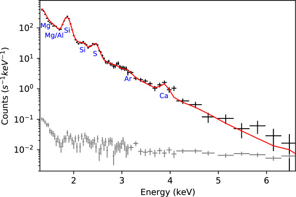
Figure 10: XSM averaged spectrum at 9:12 UT, near the peak, with the predicted spectrum (red) based on the AIA EM.

To obtain a DEM from the AIA data it is necessary to adopt a set of chemical abundances. Note that the AIA bands are dominated by Fe lines, while the XRT filters have contributions from Fe, Ne, O, Mg, and other elements. XSM can reliably measure the Si abundance, but also provides abundances for other elements. We performed an analysis of the XSM spectra around 9:12 UT and from the line to continuum we obtained for Si, Mg, Al, and S, the following absolute abundances: 7.7, 7.5, 6.5, and 7.1 dex. The Mg, Al, and S are close to the photospheric values, while the Si abundance is between photospheric (7.51 dex) and the Del Zanna (2013a) coronal value (8.0 dex). We used these values for the DEM analysis.

For the other elements we have assumed the hybrid abundances tabulated in the CHIANTI file "sun_coronal_fludra_1999_ext.abund", as they provide an intermediate FIP fractionation which is close to the results obtained from the low-FIP Si and the mid-FIP S, used as a proxy for the high-FIP elements. For example, the Fe hybrid abundance is 7.83 dex (i.e. between the photospheric value of 7.50 and the coronal value of 8.0 dex, as Si), and the O, Ne hybrid abundances are actually close to the photospheric values recommended by Asplund et al. (2009).

The resulting column EM values for a range of temperatures are shown in Fig. 8 (bottom). We note that the high temperatures are not well constrained, as the only hot channel with signal was the AIA 94 Å. For this reason, the maximum temperature for the inversion was set to log $T$[K]=6.9.

From the column EM values we calculated a volume EM by averaging the emission measures over the core of the microflare, in a region covering 100 * 50 pixels in the x and y direction, respectively. The resulting volume EM is shown in Fig. 9. We then used this volume EM to predict the XSM spectrum, which is shown, together with the observed one, in Fig. 10. There is excellent agreement between the two, indicating a reliable cross-calibration between AIA and XSM.

We then preformed forward modelling of the XRT signal, using the same EM and chemical abundances. We obtained 222 and 1019 DN/s for the Be-thin and Al-Poly filters, respectively. This results in a ratio of 0.22, equivalent to an isothermal temperature of 4 MK, nearly the same value obtained from the filter ratio. We note that adopting a very different set of chemical abundances does not change the result. In fact, with the photospheric values recommended by Asplund et al. (2009) or with the Feldman (1992) coronal values we obtain a ratio of 0.23, i.e. still 4 MK.

4 Discussion and conclusions

After a multi-wavelength survey of dozens of microflares and B-class flares during the first period of operation of the XSM monitor, it became clear how difficult it is to obtain reliable measurements of these weak, fast evolving events. XSM X-ray spectra have been great at providing an overview of how common microflares are in AR cores (even though many small heating events also occur outside ARs). Given its medium resolution, a multi-temperature analysis is difficult. However, the instrument has the great capability to measure the absolute chemical abundances for flares of B-class or above.

Trying to catch a flare with a slit spectrometer such as EIS is notoriously difficult, especially for microflares, as they only last 10 minutes or so. The information that can be telemetered is also limited, so are the diagnostics. On the basis of the present analysis, we developed and tested new EIS observing sequences for additional diagnostics.

During the multi-wavelength campaign, we also learned how to adjust the AEC to avoid saturation in the XRT filters as much as possible. On the basis of the present analysis, we have run new XRT observing sequences with different filters, as the Be-thin/Al-Poly provides isothermal temperatures which are much lower than the peak values. With a direct comparison between simultaneous EIS and XRT observations we were able to explain this result, due to the sensitivity of the Al-Poly filter to lower temperatures. The improved XRT observations will be discussed in a following paper.

One important result of our analysis regards the quiescent AR core emission during its disk crossing, which was found to have a distribution of temperatures and chemical abundances that did not change significantly over time. The XRT, EIS and XSM observations were all consistent with each other.

Most of the emission in the AR core was around 1.5 and 3 MK. As the XSM signal was dominated by the AR core, we were also able to obtain another result: the XSM spectra during quiescence indicate a FIP bias of about 2.5$\pm$0.2, adopting the silicon value. This result is important, as previous measurements did not clearly assess if it was the low-FIP elements that are enhanced in AR cores or the high-FIP ones to be depleted, relative to their photospheric values. The EIS observations indicate that the Fe/Si vs. Ar/S abundances are increased by about a factor of about 3 over the photospheric value. Combining the XSM and EIS results therefore indicates that the argon and sulphur abundances are slightly below their photospheric values. Such observations fit the nanoflare-heated scenario, where high-frequency nanoflares cause this relatively steady basal heating, and the Alfven waves excited by them cause the chemical fractionation. In fact, in the physical model discussed by Laming et al. (2019), a closed magnetic loop behaves as a resonant cavity, where the waves bounce from footpoint to the other, with a travel time that is an integral number of the wave half periods. In such case, the ponderomotive force creates a fractionation of the elements at the top of the chromosphere, where most of the hydrogen is ionized, and elements with a FIP around 10 eV such as sulphur are predicted to behave as the high-FIP elements.

In our previous study (Mondal et al., 2021), we used XSM data to show for the first time that chemical abundances of low-FIP elements quickly decrease towards photospheric values in B-class flares, with a return towards coronal values during the gradual phase. AR 12759 produced many such flares during its disk crossing, but clearly such variations did not affect the abundances of the AR core. In our previous paper, we have suggested possible reasons for such abundance variations, pointing out the need for a model to explain the observations.

It may well be that the same physical processes (e.g. magnetic reconnection in the corona) heat the basal AR cores and the flare loops, but produce very different signatures: low-energy and high-frequency nanoflares would slowly evaporate already fractionated plasma from the top of the chromosphere, while B-class flares deposit their energy deeper in the chromosphere, causing a faster evaporation of un-fractionated plasma.

The abundance variations during a flare could be used as a diagnostic to assess if the low-energy tail of the distribution of microflares is causing the basal active region heating. Ideally, one would therefore want to see if also microflares have similar abundance variations as B-class flares. If they do, this would be an argument in favor of microflares not contributing to the basal AR core heating.

One of our aims was to provide estimates of the spatial and temperature distribution of the flare loops producing the XSM signal using multi-wavelength observations, to complement the analysis of the X-ray full-Sun spectra. The information on the spatial distribution is provided by the AIA and XRT, but the temperature distribution turned out to be difficult to estimate. The AIA analysis was limited, with only one hot band responding to the flare (the 94 Å). Assuming a continuous multi-thermal emission, we obtained from AIA a strong peak around 3 MK and a secondary (flare) emission around 6-7 MK. The 3 MK emission is mostly background/foreground quiescent emission of the AR core. We are encouraged by the excellent agreement between the X-ray XSM spectra as predicted from the AIA DEM modelling and the observed values, especially considering the uncertainty in the AIA calibration. However, the isothermal approximation fits the XSM spectra equally well to a multi-thermal distribution. Clearly, the isothermal temperatures from the XSM analysis are more representative of the ‘true’ peak flare temperatures than those from the XRT Be-thin/Al-Poly filter ratio, as the latter has a bias towards the lower temperatures. However, multi-thermal emission is clearly present and should be taken into account whenever suitable observations are available.

Better estimates of the temperature distribution can be obtained from spectroscopic observations or from AIA when temperatures well above 7 MK are present, as Fe XXI becomes visible in the AIA 131 Å (and also Fe XXIV in the 193 Å band). Also, the XSM spectra of higher-T flares are very different, not just in terms of slope of the continuum, but also in terms of line emission.

In some respects we were surprised to see a low maximum temperature of about 6-7 MK from this B-class flare, as smaller flares often do produce much higher temperatures, as in the Del Zanna et al. (2011) example. In this case it is clear that the higher GOES class is simply due to the presence of an extended set of flare loops, which fits with the conclusions on the C-class flares by Bowen et al. (2013) that flares with larger volumes have lower maximum temperatures.

Further improvements on our understanding of small flares is achievable with current instrumentation and modelling, but as we mentioned in the introduction, key new high-resolution spectroscopic observations are needed.

Appendix A Further details

Fig. 11 shows the two DEMs for the AR core observed on 2020 Apr 4 and 8 obtained from Hinode EIS, while Tables A,A provide the details.

Figure 11: DEM for the AR core observed on 2020 Apr 4 and 8 obtained from Hinode EIS. The points are plotted at the temperature $T_{\rm max}$, and at the theoretical vs. the observed intensity ratio multiplied by the DEM value.

Table 3: List of emission lines from the 2020 Apr 4 active region core. $\lambda_{\rm obs}$ (Å) is the measured wavelength. DN is the number of total counts in the line, while $I_{\rm obs}$ is the calibrated radiance (phot cm^-2 s^-1 arc-second^-2) obtained with our new EIS calibration. $T_{\rm max}$ and $T_{\rm eff}$ are the maximum and effective temperature (log values in K), $R$ the ratio between the predicted and observed radiances, Ion and $\lambda_{\rm exp}$ (Å) the main contributing line, and $r$ the fractional contribution to the blend.

Table 4: List of emission lines from the 2020 Apr 8 active region core. $\lambda_{\rm obs}$ (Å) is the measured wavelength. DN is the number of total counts in the line, while $I_{\rm obs}$ is the calibrated radiance (phot cm^-2 s^-1 arc-second^-2) obtained with our new EIS calibration. $T_{\rm max}$ and $T_{\rm eff}$ are the maximum and effective temperature (log values in K), $R$ the ratio between the predicted and observed radiances, Ion and $\lambda_{\rm exp}$ (Å) the main contributing line, and $r$ the fractional contribution to the blend.

Appendix B EIS calibration

A DEM analysis was applied to off-limb quiet Sun observations close in time to the observations discussed here, to obtain the relative EIS calibration using the strongest coronal lines. The advantage is that the plasma is nearly isothermal and isodensity, and removes from the coronal lines blending with cool lines. This is an extension of the method used by Warren et al. (2014), where strict isothermality was assumed. The line ratio method adopted in Del Zanna (2013b) was also extended, using both quiet Sun and Active region observations. The calibration relative to AIA was also assessed, as was AIA against SDO EVE. Further details are given in Del Zanna and Warren (2022).

Appendix C XRT forward modelling

Fig. 12 shows the simulated XRT signal for the quiescent AR core on Apr 8.

Figure 12: Simulated XRT signal for the quiescent AR core on Apr 8.

References

- Acton et al. (1980) Acton, L. W., Finch, M. L., Gilbreth, C. W., et al. 1980, Sol. Phys., 65, 53, doi: 10.1007/BF00151384
- Arnaud (1996) Arnaud, K. A. 1996, in Astronomical Society of the Pacific Conference Series, Vol. 101, Astronomical Data Analysis Software and Systems V, ed. G. H. Jacoby & J. Barnes, 17
- Asplund et al. (2009) Asplund, M., Grevesse, N., Sauval, A. J., & Scott, P. 2009, ARA&A, 47, 481, doi: 10.1146/annurev.astro.46.060407.145222
- Bowen et al. (2013) Bowen, T. A., Testa, P., & Reeves, K. K. 2013, ApJ, 770, 126, doi: 10.1088/0004-637X/770/2/126
- Cheung et al. (2015) Cheung, M. C. M., Boerner, P., Schrijver, C. J., et al. 2015, ApJ, 807, 143, doi: 10.1088/0004-637X/807/2/143
- Cooper et al. (2020) Cooper, K., Hannah, I. G., Grefenstette, B. W., et al. 2020, ApJ, 893, L40, doi: 10.3847/2041-8213/ab873e
- Culhane et al. (2007) Culhane, J. L., Harra, L. K., James, A. M., et al. 2007, Sol. Phys., 60, doi: 10.1007/s01007-007-0293-1
- Del Zanna (1999) Del Zanna, G. 1999, PhD thesis, University of Central Lancashire, UK
- Del Zanna (2013a) —. 2013a, A&A, 558, A73, doi: 10.1051/0004-6361/201321653
- Del Zanna (2013b) —. 2013b, A&A, 555, A47, doi: 10.1051/0004-6361/201220810
- Del Zanna et al. (2021) Del Zanna, G., Andretta, V., Cargill, P. J., et al. 2021, Frontiers in Astronomy and Space Sciences, 8, 33, doi: 10.3389/fspas.2021.638489
- Del Zanna et al. (2021) Del Zanna, G., Dere, K. P., Young, P. R., & Landi, E. 2021, ApJ, 909, 38, doi: 10.3847/1538-4357/abd8ce
- Del Zanna & Mason (2014) Del Zanna, G., & Mason, H. E. 2014, A&A, 565, A14, doi: 10.1051/0004-6361/201423471
- Del Zanna & Mason (2018) —. 2018, Living Reviews in Solar Physics, 15
- Del Zanna et al. (2011) Del Zanna, G., Mitra-Kraev, U., Bradshaw, S. J., Mason, H. E., & Asai, A. 2011, A&A, 526, A1, doi: 10.1051/0004-6361/201014906
- Del Zanna et al. (2015) Del Zanna, G., Tripathi, D., Mason, H., Subramanian, S., & O’Dwyer, B. 2015, A&A, 573, A104, doi: 10.1051/0004-6361/201424561
- Duncan et al. (2021) Duncan, J., Glesener, L., Grefenstette, B. W., et al. 2021, ApJ, 908, 29, doi: 10.3847/1538-4357/abca3d
- Feldman (1992) Feldman, U. 1992, Phys. Scr, 46, 202, doi: 10.1088/0031-8949/46/3/002
- Feldman et al. (1996) Feldman, U., Doschek, G. A., Behring, W. E., & Phillips, K. J. H. 1996, ApJ, 460, 1034, doi: 10.1086/177030
- Hannah et al. (2019) Hannah, I. G., Kleint, L., Krucker, S., et al. 2019, ApJ, 881, 109, doi: 10.3847/1538-4357/ab2dfa
- Kirichenko & Bogachev (2017) Kirichenko, A. S., & Bogachev, S. A. 2017, ApJ, 840, 45, doi: 10.3847/1538-4357/aa6c2b
- Laming (2015) Laming, J. M. 2015, Living Reviews in Solar Physics, 12, 2, doi: 10.1007/lrsp-2015-2
- Laming (2017) —. 2017, ApJ, 844, 153, doi: 10.3847/1538-4357/aa7cf1
- Laming et al. (2019) Laming, J. M., Vourlidas, A., Korendyke, C., et al. 2019, ApJ, 879, 124, doi: 10.3847/1538-4357/ab23f1
- Lemen et al. (2012) Lemen, J. R., Title, A. M., Akin, D. J., et al. 2012, Sol. Phys., 275, 17, doi: 10.1007/s11207-011-9776-8
- Mithun et al. (2020) Mithun, N. P. S., Vadawale, S. V., Sarkar, A., et al. 2020, Sol. Phys., 295, 139, doi: 10.1007/s11207-020-01712-1
- Mithun et al. (2021) Mithun, N. P. S., Vadawale, S. V., Patel, A. R., et al. 2021, Astronomy and Computing, 34, 100449, doi: 10.1016/j.ascom.2021.100449
- Mitra-Kraev & Del Zanna (2019) Mitra-Kraev, U., & Del Zanna, G. 2019, A&A, 628, A134, doi: 10.1051/0004-6361/201834856
- Mondal et al. (2021) Mondal, B., Sarkar, A., Vadawale, S. V., et al. 2021, arXiv e-prints, arXiv:2107.07825
- Moore et al. (2018) Moore, C. S., Caspi, A., Woods, T. N., et al. 2018, Sol. Phys., 293, 21, doi: 10.1007/s11207-018-1243-3
- Reva et al. (2018) Reva, A., Ulyanov, A., Kirichenko, A., Bogachev, S., & Kuzin, S. 2018, Sol. Phys., 293, 140, doi: 10.1007/s11207-018-1363-9
- Shanmugam et al. (2020) Shanmugam, M., Vadawale, S. V., Patel, A. R., et al. 2020, Current Science, 118, 45, doi: 10.18520/cs/v118/i1/45-52
- Shimizu (1995) Shimizu, T. 1995, PASJ, 47, 251
- Vadawale et al. (2014) Vadawale, S., Shanmugam, M., Acharya, Y., et al. 2014, Advances in Space Research, 54, 2021 , doi: https://doi.org/10.1016/j.asr.2013.06.002
- Vadawale et al. (2021a) Vadawale, S. V., Mithun, N. P. S., Mondal, B., et al. 2021a, The Astrophysical Journal Letters, 912, L13, doi: 10.3847/2041-8213/abf0b0
- Vadawale et al. (2021b) Vadawale, S. V., Mondal, B., Mithun, N. P. S., et al. 2021b, The Astrophysical Journal Letters, 912, L12, doi: 10.3847/2041-8213/abf35d
- Warren et al. (2014) Warren, H. P., Ugarte-Urra, I., & Landi, E. 2014, ApJS, 213, 11, doi: 10.1088/0067-0049/213/1/11
- Winebarger et al. (2012) Winebarger, A. R., Warren, H. P., Schmelz, J. T., et al. 2012, ApJ, 746, L17, doi: 10.1088/2041-8205/746/2/L17
- Woods et al. (2017) Woods, T. N., Caspi, A., Chamberlin, P. C., et al. 2017, ApJ, 835, 122, doi: 10.3847/1538-4357/835/2/122