Predicting polaron mobility in organic semiconductors with the Feynman variational approach

Abstract

We extend the Feynman variational approach to the polaron problem [1] to the Holstein (lattice) polaron. This new theory shows a discrete transition to small-polarons is observed in the Holstein model.

The method can directly used in the FHIP [2] mobility theory to calculate dc mobility and complex impedance. We show that we can take matrix elements from electronic structure calculations on real materials, by modelling charge-carrier mobility in crystalline rubrene. Good agreement is found to measurement, in particular the continuous thermal transition in mobility from band-like to thermally-activated, with a minimum in mobility predicted at 140 K.

I Introduction

Polarons are the quasi-particles formed by an electron (or hole) interacting with a polar material. The dielectric response of the material (an electron-phonon coupling) tries to localise the charge-carrier. If the coupling is relatively weak, the polaron is adiabatically connected to the free carrier Bloch state, and we can apply perturbation theory to this delocalised state, for instance to evaluate mobility. Momentum is a well defined quantum number (charge transport is coherent). Charge carrier mobility reduces with increasing temperature due to increased scattering from the increasingly disordered lattice. If the electron-phonon coupling is strong, the electron (or hole) is localised to a small region. Charge transport becomes incoherent, and occurs by temperature activated hopping.

In organic electronic materials, with the understanding that the charge-carrier state is a small polaron. This is often modelled with semi-classical transfer rate theories as a classical object hopping from site to site. (Note that these theories look very different from the band-theory perturbation approach outlined above.) The matrix elements which parameterise these rate equations can be calculated, within certain approximations, from electronic-structure calculations, but it is a challenge (and often an input to the simulation and calculations) to define the sites on which the charge carriers are localised.

More recently transient localisation theory [3] attempts to correct band-transport theory with the presence of incoherent states,

To go beyond these limitations, a direct solution of the non-adiabatic dynamics is required. This becomes a full quantum-field problem as in the most simple case you are simulating a single electron, but interacting with an infinite field of vibrations (phonon quantisations).

Recently Giannini and coworkers [4, 5] have developed a non-adiabatic surface-hopping based method, combined with electronic structure evaluation of the adiabatic and non-adiabatic electron transfer integrals, to predict mobility in crystalline semiconductors. A limitation of the method is that the simulation box must be sufficient to fully enclose the charge-carrier state [5], and then the mobility is inferred by diffusion.

Chang et al. [6] recently developed a cumulant expansion of many-body-perturbation-theory combined with a linear response mobility method, to estimate the temperature-dependent electron mobility in crystalline Napthalene.

A polaron theory which applies from weak to strong coupling is the celebrated Feynman variational approximation [1]. Formulated in the model Fröhlich Hamiltonian for a continuum polaron with dielectrically mediated electron-phonon coupling (e.g. the infrared activity of phonon modes), this variational theory is accurate to a few percent in energy from weak to strong coupling. The method is based in the path-integral formulation of quantum mechanics, where the infinite degree of freedom of the phonon field is integrated out. The Lagrangian action associated with the true Fröhlich Hamiltonian cannot be analytically integrated over, so instead a variational quasi-particle solution is made of the electron (hole) attached by a spring to a fictitious mass. This fictitious mass represents the phonon drag term.

The FHIP theory [2] builds on this variational solution, providing a linear response (relatively low field) mobility theory. The interacting thermal bath of harmonic phonon excitations is replaced with a two-point memory function. Thereby a mobility theory is developed which contains all orders of perturbation theory. In crystalline semiconductors, these techniques are being increasing recognised as powerful and predictive , not least as polar optical mode scattering (i.e. polaronic effects) are recognised as a major scattering process across a wide range of technologically relevant materials.

In the FHIP theory, the object around which the mobility is constructed is just the variational solution of the polaron quasiparticle, i.e. Fröhlich’s Hamiltonian doesn’t explicitly occur. Corrections to this solution are then made by expanding around the influence function for the quasi-particle with the influence functional derived from the Fröhlich Hamiltonian. This quasi-particle solution is simply the two variational parameters $v$ and $w$ (or equivalently, the fictitious mass $M$ and spring coupling constant $C$).

It is well known [7, 8] that the FHIP theory works equally well with the finite temperature Ōsaka [9] extension to Fröhlich’s Hamiltonian, even though the parameters of the variational solution are observed to be quite different [8]. This begs the question whether the FHIP theory can apply equally well to other quasi-particle mobility problems, and whether the original Feynman variational solution can be extended beyond Fröhlich’s Hamiltonian to other electron-phonon couplings.

We thought it would be a good idea to see whether we could apply these polaron variation theories to organic electronic materials, where the polaron problem is treated on a lattice of individual sites (rather than a continuum), with Holstein (on site) and Peierls (off site) electron-phonon couplings, rather than the dielectric electron-phonon coupling in the Fröhlich Hamiltonian (the physics of a polar continuum).

For simplicity and as an example of the theory, we only consider rubrene in the applications section of this paper, a high mobility organic crystal. There are many measures of charge-carrier mobility , as well as many attempts to simulate the mobility . Of particular use to us is a calculation of electron-phonon coupling [10], presented in the language and terms of solid-state physics.

II Theory

II.1 Polaron theories

Kornilovitch and coworkers studied the lattice polaron in both the Holstein-Peierls [11] and Fröhlich [12] form. Their key approach [13] is to use the Feynman trick [1] of integrating over the phonon field, but evaluate the path-integral construction of the partition function with Monte-Carlo.

Coropceanu et al. [14] provide a review of the standard approaches to calculating charge transfer parameters in organic semiconductors. Most organic semiconductors are highly disordered or amorphous, so that the starting point for a calculation of charge carrier mobility is the transfer of an electron between two discrete molecules in vacuum.

II.2 Marcus theory of small polaron hopping

Marcus theory [15] is the standard approach used to model small-polaron hopping transport in organic semiconductors [16]. The theory models the high-temperature limit of thermally activated hopping. This reorganisation energy can be understood as the electron phonon coupling. The reorganisation energy is split into, using the terms of Marcus theory developed for solvated reactions, inner and outer sphere reorganisation energies. Jortner [17] shows how the semi-classical Marcus theory can be made consistent with the low-temperature quantum mechanical tunneling limit.

The inputs to the theory, which can be calculated with electronic structure techniques, are the transfer integral (kinetic energy) between the electron localised on the two states, and a reorganisation energy.

The inner sphere reorganisation energy, for a molecular semiconductor, is driven by the change in bond lengths of the molecule upon charging and discharging. This is equivalent to the Holstein (same site) electron-phonon coupling.

The outer-sphere reorganisation energy contains contributions from vibration driven fluctuation in the transfer integral, and is equivalent to the Peierls (off site) electron-phonon coupling.

II.3 Calculation of band structure

The electronic coupling between organic electronic materials is usually described in terms of a transfer integral (hopping matrix element) between two adiabatic states localised on nearest-neighbour molecules. Polaron theories based in a band description instead consider a band-structure of Bloch states as their starting point, with an associated effective mass that describes the quadratic dispersion relationship observed near the extremal points.

To link these concepts, we use a simple tight-binding model of the electronic structure. In one dimension, the coupling $t$ between successive lattice locations (rubrene molecules in our example) gives rise to a dispersion relation (band structure),

$$E(k;t,a)=\epsilon_{0}-2zt\cos(ka).$$ (1)

where $z$ is the number of nearest neighbouring lattice sites and $a$ is the lattice constant. Expanding around $k=0$ using the identity $\cos(\theta)\approx 1-\frac{\theta^{2}}{2}\quad;\quad\theta\ll 1$, and by analogy with the free electron dispersion relationship $E(k)=\frac{p^{2}}{2m_{e}}=\frac{\hbar^{2}k^{2}}{2m_{e}}$ we have the tight-binding effective mass as,

$$m^{*}=\frac{\hbar^{2}}{zta^{2}}.$$ (2)

II.4 Calculation of electron-phonon couplings

The reorganisation energy, often calculated with the ’four point’ method by considering the relaxation of a molecule in its charged and uncharged states, can also be composed of the sum of individual phonon modes and their dimensionless electron-phonon coupling,

$$\lambda=\sum_{i}^{N}\hbar\omega_{i}g_{i}.$$ (3)

Where the sum is over N phonon (vibrational) modes, $\hbar$ the reduced Planck constant, $\omega_{i}$ the reduced frequency of the $i$’th mode, $g_{i}$ the dimensionless electron-phonon coupling of the $i$’th mode.

Additionally this can be split into an ‘inner sphere’, and ‘outer sphere’ reorganisation energy which are equivalent to the Holstein (on site / intramolecular) and Peierls (off site / intermolecular) electron-phonon couplings.

Marcus theory makes an adiabatic approximation and assumes that the rate of electron transfer is slow relatively to the vibrational $w_{i}$ degrees of freedom, and so this information is not required. The Feynman theory explicitly considers the exchange of energy between the electron and the vibrational degrees of freedom, and so it is essential that we retain information about $w_{i}$, at least in some ‘effective frequency’ approach as done by Hellwarth et al. [7].

III Extending the Feynman variational polaron theory to the Holstein polaron

Following the notation of Kornilovitch [13], we write the general electron-phonon (e-ph) Hamiltonian as

$$H= -t\sum_{\langle\mathbf{n}\mathbf{n^{\prime}}\rangle}c^{\dagger}_{\mathbf{n^{\prime}}}c_{\mathbf{n}}+\sum_{\mathbf{m}}\left(-\frac{\hbar^{2}}{2M}\frac{\partial^{2}}{\partial\xi^{2}_{\mathbf{m}}}+\frac{M\omega^{2}}{2}\xi^{2}_{\mathbf{m}}\right)$$ (4)

$$-\sum_{\mathbf{n}\mathbf{m}}f_{\mathbf{m}}(\mathbf{n})c^{\dagger}_{\mathbf{n}}c_{\mathbf{n}}\xi_{\mathbf{m}}.$$

Here, $c_{\mathbf{n}}^{\dagger}$ ($c_{\mathbf{n}}$) are the creation (annihilation) operators for a Wannier electron at lattice site $\mathbf{n}$. $\xi_{\mathbf{m}}$ is the displacement of an ion at lattice site $\mathbf{m}$, where the ion displacements are approximated as independent Einstein oscillators with mass $M$ and frequency $\omega$. $t$ is the electronic coupling between successive lattice sites. $f_{\mathbf{m}}(\mathbf{n})$ is the electron-phonon interaction between an electron $\mathbf{n}$ and ion $\mathbf{m}$.

The electron-phonon interaction $f_{\mathbf{m}}(\mathbf{n})$ is localised to a specific lattice site using a Kronecker-delta function for the Holstein model,

$$f_{\mathbf{m}}(\mathbf{n})=\kappa_{\text{H}}\delta_{\mathbf{m}\mathbf{n}},$$ (5)

where $\kappa_{H}$ is the Holstein electron-phonon coupling strength. The electron-phonon interaction is long-range for the (dielectrically mediated) Fröhlich model,

$$f_{\mathbf{m}}(\mathbf{n}) =\kappa_{\text{F}}\frac{\exp\left(i\mathbf{m}\cdot\mathbf{n}\right)}{\absolutevalue{\mathbf{m}}},$$ (6)

where $\kappa_{F}$ is the Fröhlich electron-phonon coupling strength.

III.1 The electron-phonon path integral

We simplify the electron-phonon Hamiltonian (Eqn. 4) to the case of just one electron. The real-space path integral corresponding to this electron-phonon Hamiltonian is given by Kornilovitch’s shifted partition function [18],

$$Z_{\Delta\mathbf{r}} =\int_{\mathbf{r}(0)=\mathbf{r}_{i}}^{\mathbf{r}(\hbar\beta)=\mathbf{r}_{i}+\Delta\mathbf{r}}\mathcal{D}^{3}r(\tau)\int_{\xi(0)=\xi_{\mathbf{m}}}^{\xi(\hbar\beta)=\xi_{\mathbf{m}-\Delta\mathbf{r}}}\mathcal{D}\xi_{\mathbf{m}}(\tau)$$ (7)

$$\times\exp\left(-S\left[\mathbf{r}(\tau),\xi_{\mathbf{m}}(\tau)\right]/\hbar\right),$$

where the electron has moved by the shift vector $\Delta\mathbf{r}$. The electron-phonon action is

$$S[\mathbf{r}(\tau),\xi_{\mathbf{m}}(\tau)] =\frac{m^{*}}{2}\int_{0}^{\hbar\beta}d\tau\ \dot{\mathbf{r}}^{2}(\tau)$$ (8)

$$+\sum_{\mathbf{m}}\int_{0}^{\hbar\beta}d\tau\left[\frac{M\dot{\xi}^{2}_{\mathbf{m}}(\tau)}{2\hbar^{2}}+\frac{M\omega^{2}}{2}\xi^{2}_{\mathbf{m}}(\tau)\right]$$

$$-\sum_{\mathbf{m}}\int_{0}^{\hbar\beta}d\tau\ f_{\mathbf{m}}\left[\mathbf{r}(\tau)\right]\xi_{\mathbf{m}}(\tau).$$

The path integral over the ion displacements $\xi_{\mathbf{m}}(\tau)$ is Gaussian and can be evaluated analytically. The result is a time retarded self-interaction acting on the electron,

$$S_{\text{pol}}[\mathbf{r}(\tau)] =\frac{m^{*}}{2}\int_{0}^{\hbar\beta}d\tau\ \dot{\mathbf{r}}^{2}(\tau)$$ (9)

$$-\frac{1}{4\omega M}\int_{0}^{\hbar\beta}d\tau\int_{0}^{\hbar\beta}d\tau^{\prime}\ g_{\omega}(\absolutevalue{\tau-\tau^{\prime}})$$

$$\times\Phi\left[\mathbf{r}(\tau),\mathbf{r}(\tau^{\prime})\right],$$

where the phonon propagator is

$$g_{\omega}(\tau)=\frac{\cosh\left(\omega\left[\hbar\beta/2-\tau\right]\right)}{\sinh\left(\hbar\omega\beta/2\right)},$$ (10)

and self-interaction functional is

$$\Phi\left[\mathbf{r}(\tau),\mathbf{r}(\tau^{\prime})\right]=\sum_{\mathbf{m}}f_{\mathbf{m}}\left[\mathbf{r}(\tau)\right]f_{\mathbf{m}}\left[\mathbf{r}(\tau^{\prime})\right].$$ (11)

The action in the shifted partition function actually has two additional terms due to the boundary condition that the end of the ion paths $\xi_{\mathbf{m}}(\hbar\beta)$ are shifted relative to the start of the path $\xi_{\mathbf{m}}(0)$ by the change in the electron coordinate $\Delta\mathbf{r}$. The shift in the ions must be the same as that of the electron, so we require $\xi_{\mathbf{m}}(\hbar\beta)=\xi_{\mathbf{m}-\Delta\mathbf{r}}(0)$ [13]. However, we assume for simplicity that we have periodic boundary conditions $\xi_{\mathbf{m}}(\hbar\beta)=\xi_{\mathbf{m}}(0)$ such that $\Delta\mathbf{r}=0$ and so these extra terms are absent. We now have just the usual thermodynamic partition function, $Z_{\Delta\mathbf{r}=0}=Z$, corresponding to the action given in Eqn. (9).

For the Fröhlich model the self-interaction functional is

$$\Phi_{\text{Fr\"{o}hlich}}\left[\mathbf{r}(\tau),\mathbf{r}(\tau^{\prime})\right] =\lim_{\Omega_{0}\to\infty}\sum_{\mathbf{m}}\frac{\kappa_{F}^{2}}{\absolutevalue{\mathbf{m}}^{2}}e^{i\mathbf{m}\cdot\left(\mathbf{r}(\tau)-\mathbf{r}(\tau^{\prime})\right)}$$ (12)

$$=\kappa_{\text{F}}^{2}\Omega_{0}\int\frac{d^{3}m}{(2\pi)^{3}}\frac{e^{i\mathbf{m}\cdot\left(\mathbf{r}(\tau)-\mathbf{r}(\tau^{\prime})\right)}}{\absolutevalue{\mathbf{m}}^{2}}$$

$$=\frac{\kappa_{\text{F}}^{2}}{\absolutevalue{\mathbf{r}(\tau)-\mathbf{r}(\tau^{\prime})}},$$

where $0\leq\absolutevalue{m}<\infty$. The Fröhlich model makes the continuum approximation of the lattice, $\lim_{\Omega_{0}\to\infty}\sum_{\mathbf{m}}\sim\Omega_{0}\int d^{3}m/(2\pi)^{3}$, where $\Omega_{0}$ is the unit-cell volume.

For the Holstein model the self-interaction functional is

$$\Phi_{\text{Holstein}}\left[\mathbf{r}(\tau),\mathbf{r}(\tau^{\prime})\right] =\kappa_{H}^{2}\sum_{\mathbf{m}}\delta_{\mathbf{m}\mathbf{r}(\tau)}\delta_{\mathbf{m}\mathbf{r}(\tau^{\prime})}$$ (13)

$$=\kappa_{H}^{2}\delta_{\mathbf{r}(\tau)\mathbf{r}(\tau^{\prime})}$$

$$=\kappa_{H}^{2}\Omega_{0}\int\frac{d^{3}m}{(2\pi)^{3}}e^{i\mathbf{m}\cdot\left(\mathbf{r}(\tau)-\mathbf{r}(\tau^{\prime})\right)},$$

where $0\leq\absolutevalue{m}\leq k_{c}$, $k_{c}=2\pi/a$ is an ultraviolet momentum cutoff and $a$ is the lattice constant.

III.2 Finite temperature variational method

The variational method for the polaron developed by Feynman gives a lower upper-bound to the polaron free energy,

$$F \leq F_{0}(\beta)-\frac{1}{\hbar\beta}\langle S_{\text{pol}}-S_{0}\rangle_{0}$$ (14)

$$\leq F_{0}(\beta)$$

$$-\frac{1}{4\hbar\omega\beta M}\int_{0}^{\hbar\beta}d\tau\int_{0}^{\hbar\beta}d\tau^{\prime}\ g_{\omega}(\absolutevalue{\tau-\tau^{\prime}})\langle\Phi_{\text{pol}}-\Phi_{0}\rangle_{0},$$

where the expectation $\langle\mathcal{O}\rangle_{0}$ is defined as

$$\langle\mathcal{O}\rangle_{0}\equiv\frac{\int\mathcal{D}^{3}r(\tau)\mathcal{O}e^{-S_{0}[\mathbf{r}(\tau)]}}{\int\mathcal{D}^{3}r(\tau)e^{-S_{0}[\mathbf{r}(\tau)]}},$$ (15)

and $S_{0}[\mathbf{r}(\tau)]$ is a trial action that is chosen to best approximate the model action $S_{\text{pol}}[\mathbf{r}(\tau)]$ and where the path integral for $S_{0}$ can be analytically evaluated. The trial action is typically chosen to be quadratic in the electron coordinate $\mathbf{r}(\tau)$ for this reason.

We use the standard quasi-particle ’trial action’ for the electron-phonon lattice model,

$$S_{0}[\mathbf{r}(\tau)] =\frac{m^{*}}{2}\int_{0}^{\hbar\beta}d\tau\ \dot{\mathbf{r}}^{2}(\tau)$$ (16)

$$+\frac{C}{2}\int_{0}^{\hbar\beta}d\tau\int_{0}^{\hbar\beta}d\tau^{\prime}\ g_{\omega w}(\absolutevalue{\tau-\tau^{\prime}})$$

$$\times\Phi_{0}\left[\mathbf{r}(\tau),\mathbf{r}(\tau^{\prime})\right],$$

where the trial self-interaction functional is quadratic,

$$\Phi_{0}[\mathbf{r}(\tau),\mathbf{r}(\tau^{\prime})]=\left[\mathbf{r}(\tau)-\mathbf{r}(\tau^{\prime})\right]^{2}.$$ (17)

All the expectation values in the variational expression can be evaluated from $\langle e^{i\mathbf{m}\cdot(\mathbf{r}(\tau)-\mathbf{r}(\tau^{\prime})}\rangle_{0}$ and gives

$$\langle e^{i\mathbf{m}\cdot(\mathbf{r}(\tau)-\mathbf{r}(\tau^{\prime}))}\rangle_{0}:=\exp\left[-m^{2}r_{p}^{2}D(\absolutevalue{\tau-\tau^{\prime}})\right]$$ (18)

where $r_{p}=\sqrt{\hbar/(2\omega m^{*})}$ is the characteristic polaron radius and the diffusion function $D(\tau)$ is given by

$$D(\tau) =\frac{w^{2}}{v^{2}}\left(\omega\tau-\frac{\omega\tau^{2}}{\hbar\beta}\right)$$ (19)

$$+\frac{v^{2}-w^{2}}{v^{3}}\frac{\cosh(\hbar\omega v\beta/2)-\cosh(\omega v[\hbar\beta/2-\tau])}{\sinh(\hbar\omega v\beta/2)}.$$

The lattice integral can then be done in spherical coordinates. For the Holstein self-interaction functional we have

$$\langle\Phi_{\text{Holstein}}\rangle_{0} =\frac{\kappa_{H}^{2}\Omega_{0}}{(2\pi)^{3}}\int_{0}^{2\pi}d\theta\ \sin(\theta)\int_{0}^{\pi}d\phi\$$ (20)

$$\times\int_{0}^{k_{c}}dk\ k^{2}e^{-k^{2}r_{p}^{2}D(\tau)}$$

$$=\frac{\kappa_{H}^{2}\Omega_{0}}{2\pi^{2}}\int_{0}^{k_{c}}dk\ k^{2}e^{-k^{2}r_{p}^{2}D(\tau)}$$

$$=\frac{\kappa_{H}^{2}}{2\sqrt{\pi}}\frac{a^{2}}{r_{p}^{2}}\frac{Y(\tau,k_{c})}{\sqrt{D(\tau)}},$$

where we define the function

$$Y(\tau,k_{c}) =\frac{\Omega_{0}}{4\pi r_{p}a^{2}}\frac{1}{D(\tau)}\text{erf}\left(k_{c}r_{p}\sqrt{D(\tau)}\right)$$ (21)

$$-\frac{k_{c}\Omega_{0}}{2\pi a^{2}}\sqrt{\frac{1}{\pi D(\tau)}}\exp\left(-k_{c}^{2}r_{p}^{2}D(\tau)\right).$$

For the Fröhlich self-interaction functional we have

$$\langle\Phi_{\text{Fr\"{o}hlich}}\rangle_{0} =\frac{\kappa_{F}^{2}\Omega_{0}}{(2\pi)^{3}}\int_{0}^{2\pi}d\theta\ \sin(\theta)\int_{0}^{\pi}d\phi\$$ (22)

$$\times\int_{0}^{\infty}dk\ e^{-k^{2}r_{p}^{2}D(\tau)}$$

$$=\frac{4\pi\kappa_{F}^{2}\Omega_{0}}{(2\pi)^{3}}\int_{0}^{\infty}dk\ e^{-k^{2}r_{p}^{2}D(\tau)}$$

$$=\frac{\kappa_{F}^{2}\Omega_{0}}{4\pi^{3/2}r_{p}}\frac{1}{\sqrt{D(\tau)}}.$$

One difference between the Holstein and Fröhlich model is in the domain of the radial reciprocal-space integral. Whereas the domain of the radial integral for the Fröhlich model is over all of reciprocal-space, it is bounded by a radius $k_{c}$ for the Holstein model, keeping the total reciprocal-space integral within a sphere of volume $(2\pi/a)^{3}$. Physically, this is a manifestation of an ultraviolet momentum cutoff due to the discrete lattice. An early attempt of our theory did not bound this integral and had an ultraviolet catastrophe and divergent integral. In the continuum Fröhlich model, the integral is convergent.

The variational inequality for the Fröhlich model is then

$$F_{\text{Fr\"{o}hlich}} \leq F_{0}(\beta)-\frac{1}{\beta}\langle S_{0}\rangle_{0}-\frac{\kappa_{F}^{2}\Omega_{0}}{16\pi^{3/2}r_{p}\hbar\omega\beta}$$ (23)

$$\times\int_{0}^{\hbar\beta}d\tau\int_{0}^{\hbar\beta}d\tau^{\prime}\ \frac{g_{\omega}(\absolutevalue{\tau-\tau^{\prime}})}{\sqrt{D(\absolutevalue{\tau-\tau^{\prime}})}},$$

where

$$\kappa_{F}=4\pi e\sqrt{\frac{2}{\Omega_{0}}},$$ (24)

and the phonon mass for the Fröhlich model is given by

$$M_{\text{Fr\"{o}hlich}}=\frac{4\pi}{\omega^{2}}\left(\frac{1}{\epsilon_{\text{optic}}}-\frac{1}{\epsilon_{\text{static}}}\right)^{-1},$$ (25)

which gives the free energy to be

$$F_{\text{Fr\"{o}hlich}} \leq F_{0}(\beta)+\frac{1}{\beta}\langle S_{0}\rangle_{0}$$ (26)

$$-\frac{\alpha\omega^{2}}{2\sqrt{\pi}\beta}\int_{0}^{\hbar\beta}d\tau\int_{0}^{\hbar\beta}d\tau^{\prime}\ \frac{g_{\omega}(\absolutevalue{\tau-\tau^{\prime}})}{\sqrt{D(\absolutevalue{\tau-\tau^{\prime}})}}.$$

where $\alpha$ is the usual dimensionless Fröhlich electron-phonon coupling parameter.

The variational inequality for the Holstein model is

$$F_{\text{Holstein}} \leq F_{0}(\beta)+\frac{1}{\beta}\langle S_{0}\rangle_{0}-\frac{\kappa_{H}^{2}}{8\sqrt{\pi}\hbar\omega\beta}\frac{a^{2}}{r_{p}^{2}}$$ (27)

$$\times\int_{0}^{\hbar\beta}d\tau\int_{0}^{\hbar\beta}d\tau^{\prime}\ \frac{g_{\omega}(\absolutevalue{\tau-\tau^{\prime}})}{\sqrt{D(\absolutevalue{\tau-\tau^{\prime}})}}Y\left(\absolutevalue{\tau-\tau^{\prime}},k_{c}\right).$$

We define the dimensionless electron-phonon coupling parameter $g$ of the Holstein model from,

$$\kappa_{H}^{2} =2Mg\omega^{2}zt$$ (28)

$$=2Mg\hbar^{2}\omega^{2}/(m^{*}a^{2})$$

$$=4Mg\hbar\omega^{3}r_{p}^{2}/a^{2},$$

where $a$ is the lattice constant and $z=2d$ is the number of nearest neighbouring lattice sites with $d$ the number of spatial dimensions. We have replaced $zt$ with the expression for the effective mass (Eqn. (2)). Substituting this gives

$$F_{\text{Holstein}} \leq F_{0}(\beta)+\frac{1}{\beta}\langle S_{0}\rangle_{0}-\frac{g\omega^{2}}{2\sqrt{\pi}\beta}$$ (29)

$$\times\int_{0}^{\hbar\beta}d\tau\int_{0}^{\hbar\beta}d\tau^{\prime}\ \frac{g_{\omega}(\absolutevalue{\tau-\tau^{\prime}})}{\sqrt{D(\absolutevalue{\tau-\tau^{\prime}})}}Y\left(\absolutevalue{\tau-\tau^{\prime}},k_{c}\right).$$

The expectation value of the trail action $\langle S_{0}\rangle_{0}$ and the free energy of the trial system $F_{0}(\beta)$ are the same for both models and are as given by Ōsaka [9]

$$\langle S_{0}\rangle_{0}=\frac{3\hbar\omega\beta}{4}\frac{v^{2}-w^{2}}{v}\left(\frac{2}{v\hbar\omega\beta}-\coth\left(\frac{v\hbar\omega\beta}{2}\right)\right),$$ (30)

and

$$F_{0}(\beta)=\frac{3}{2\beta}\log\left(2\pi\hbar\omega\beta\right)+\frac{3}{\beta}\log\left(\frac{w\sinh(\hbar\omega\beta v/2)}{v\sinh(\hbar\omega\beta w/2)}\right).$$ (31)

III.3 Zero temperature variational method

To obtain variational expressions for the ground-state energy we take the limit of the thermodynamic temperature $\beta\to\infty$. For large $\beta$, we can transform the double imaginary-time integrals using the relation

$$\int_{0}^{\hbar\beta}d\tau\int_{0}^{\hbar\beta}d\tau^{\prime}\ f(\absolutevalue{\tau-\tau^{\prime}})\sim 2\hbar\beta\int_{0}^{\hbar\beta}d\tau\ f(\tau),$$ (32)

which is valid for any function $f$ in the limit $\beta\to\infty$ [18].

We then find the variational expression for the ground-state energy of the Fröhlich model to be

$$E_{\text{Fr\"{o}hlich}}\leq\frac{3\hbar\omega}{4}\frac{\left(v-w\right)^{2}}{v}-\frac{\alpha\hbar\omega^{2}}{\sqrt{\pi}}\int_{0}^{\infty}d\tau\ \frac{e^{-\omega\tau}}{\sqrt{D_{\infty}(\tau)}},$$ (33)

where $\lim_{\beta\to\infty}g_{\omega}(\tau)=\exp(-\omega\tau)$ and $D_{\infty}(\tau)$ is the limit of $D(\tau)$ as $\beta\to\infty$ and given by

$$D_{\infty}(\tau)=\frac{w^{2}}{v^{2}}\omega\tau+\frac{v^{2}-w^{2}}{v}\left(1-e^{-v\omega\tau}\right).$$ (34)

For the Holstein model we find,

$$E_{\text{Holstein}}\leq\frac{3\hbar\omega}{4}\frac{\left(v-w\right)^{2}}{v}-\frac{g\hbar\omega^{2}}{\sqrt{\pi}}\int_{0}^{\infty}d\tau\ \frac{e^{-\omega\tau}Y_{\infty}(\tau,k_{c})}{\sqrt{D_{\infty}(\tau)}}.$$ (35)

where $Y_{\infty}(\tau,k_{c})$ is $Y(\tau,k_{c})$ in the limit $\beta\to\infty$ and is given by

$$Y_{\infty}(\tau,k_{c}) =\frac{\Omega_{0}}{4\pi r_{p}a^{2}}\frac{1}{D_{\infty}(\tau)}\text{erf}\left(k_{c}r_{p}\sqrt{D_{\infty}(\tau)}\right)$$ (36)

$$-\frac{\Omega_{0}k_{c}}{2\pi a^{2}}\sqrt{\frac{1}{\pi D_{\infty}(\tau)}}\exp\left(-k_{c}^{2}r_{p}^{2}D_{\infty}(\tau)\right).$$

It can be seen that $Y_{\infty}(\tau,k_{c})\to\frac{\Omega_{0}}{4\pi r_{p}a^{2}}\frac{1}{D_{\infty}(\tau)}$ as $k_{c}\to\infty$ since the asymptoptic limit of the error function is $1$ and the Gaussian goes to zero. However, in this limit the remaining imaginary-time integral is non-convergent as at very small imaginary-times $\tau<<1$ the integrand is proportional to $e^{-\tau}/\tau^{3/2}$ and diverges — the ultraviolet catastrophe. Therefore, the Holstein ground-state energy is only finite for finite momentum cutoffs $k_{c}$.

III.4 The polaron effective mass

I want to do this properly. If we are referencing Kornilovitch, who developed the machinery derive the effective mass properly with open-boundary conditions, I think I should do so too. Back to the math!

III.5 The polaron mobility

IV Results

IV.1 Holstein versus Fröhlich Hamiltonians

First we look at the difference of the new Holstein model, as a function of the dimensionless electron-phonon coupling parameter $\alpha$ ($g$ in the organic literature).

When we plot the polaron mass renormalisation as a function of $\alpha$ (Fig. 1) we see a sharp transition to a high effective mass regime around $\alpha=2.5$. This is a transition to a small-polaron regime where the polaron is localised. In the Feynman theory, the Fröhlich theory leads to a much more gradual transition to the trapped state around $\alpha=6$.

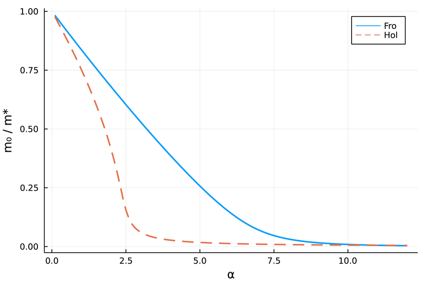
Figure 1: The (inverse) polaron effective mass as a function of dimensionless electron-phonon coupling strength $\alpha$ for the original Feynman Fröhlich theory (’Fro’) and the Holstein model (’Hol’) we present here. A sharp transition to a small-polaron is clearly observed at $\alpha=2.5$ in the Holstein model, whereas the original Feynman (Fröhlich) model shows a gentle transition to the strong-coupling regime at $\alpha=6$.

Looking directly at the variational parameters of the quasi-particle solution, $v$ and $w$, Fig. 2, we see that though the Holstein model is similarly monotonic in the variational parameters as a function of $\alpha$ they have much more structure, with a definite inflection in $v$ at $\alpha=2.5$.

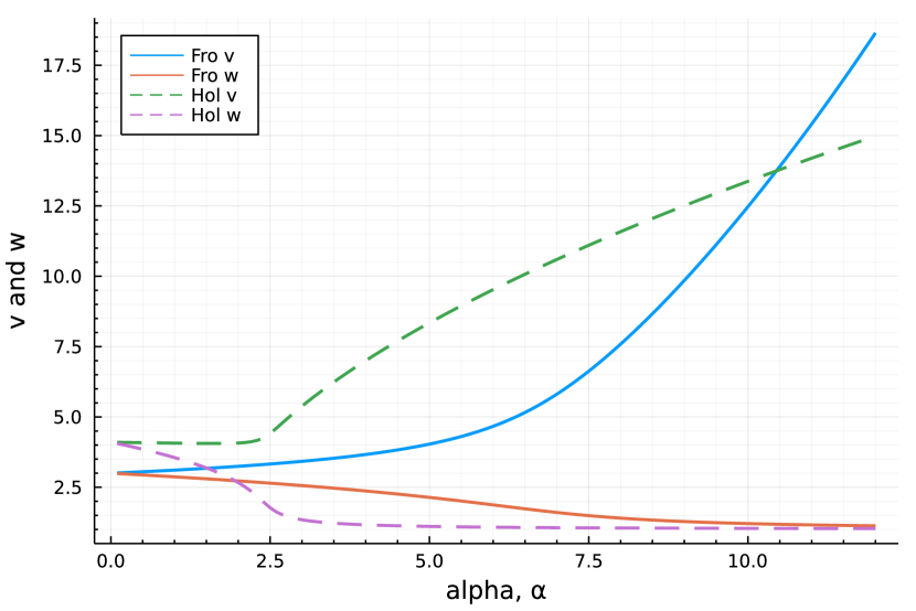
Figure 2: The Feynman polaron quasiparticle parameters, $v$ and $w$, as a function of dimensionless electron-phonon coupling strength $\alpha$ for the original Feynman Fröhlich theory (’Fro’) and the Holstein model (’Hol’) we present here.

The polaron binding energy as a function of $\alpha$ is shown in Fig. 3.

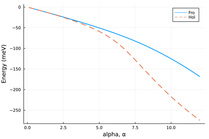
Figure 3: The Feynman polaron quasiparticle energy for rubrene, as a function of dimensionless electron-phonon coupling strength $\alpha$ for the original Feynman Fröhlich theory (’Fro’) and the Holstein model (’Hol’) we present here.

IV.2 Rubrene

We take parameters for rubrene from Ordejón et al. [10]. We lump the Peierls (off site) and Holstein (on site) contributions together as one single electron-phonon coupling, which we use in our new Holstein Hamiltonian theory, and with the standard Fröhlich Hamiltonian theory.

For simplicity we consider a single effective phonon frequency, though the method we present here could be extended to multiple phonon modes, as we have demonstrated for the Fröhlich Hamiltonian [19].

Taking the Ordejón et al. [10] effective Holstein electron-phonon interaction as $\omega_{H}=$ $1208.9\text{\,}{\mathrm{cm}}^{-1}$ $g_{H}=$ $106.8\text{\,}\mathrm{meV}$ $=0.712$; and Peierls $\omega_{P}=$ $117.9\text{\,}{\mathrm{cm}}^{-1}$ $g_{P}=$ $21.9\text{\,}\mathrm{meV}$ $=1.496$. Summing the electron-phonon couplings $g$, and taking a weighted (by the dimensionless coupling) mean of the effective phonon frequency, we have $g=\alpha=2.21$ and $\omega=$ $470\text{\,}{\mathrm{cm}}^{-1}$ $=$ $1.41\text{\,}\mathrm{THz}$.

In the athermal (low temperature) Fröhlich model this arrives at a variational solution of $v=3.31$, $w=2.66$, whereas the Holstein model produces quite a different $v=4.25$, $w=1.99$. We note that rubrene appears right on the cusp where the Holstein model goes through a transition, and so the details of the model parameters, inaccuracies in the electronic structure method, physical variations in sample, and finite temperature effects may change things considerable.

Taking our new ’S’ influence function for the Holstein model, we can generate a mobility theory following the FHIP approach. The low-temperature frequency-dependent impedance of the Holstein model has quite different structure between the Fröhlich and Holstein solutions, Fig. 4.

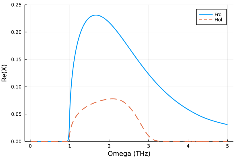
Figure 4: Our low-temperature real impedance of rubrene from the FHIP [2] theory, as a function of frequency for the original Feynman Fröhlich theory (’Fro’) and the Holstein model (’Hol’) we present here.

Looking at the temperature dependence of the variational parameters for rubrene in Fig. 5 we see quite different structure. With these finite temperature (phonon entropy) Hamiltonians following Ōsaka, we don’t have the direct mechanistic explanation of the quasi particle.

Figure 5: The Feynman polaron quasiparticle parameters for rubrene, $v$ and $w$, as a function of temperature (K) for the original Feynman Fröhlich theory (’Fro’) and the Holstein model (’Hol’) we present here.

Finally, we show the temperature dependent mobility of rubrene with the new Holstein model and the previous Fröhlich model. The Holstein model gets closer to the experimentally observed mobility of $\sim 10\text{\,}{\mathrm{cm}}^{2}\text{\,}{\mathrm{V}}^{-1}\text{\,}\mathrm{s}$. There is a much richer structure, suggesting initially a band-transport regime with mobility decreasing as a function of temperature, before transitioning around $\sim 140\text{\,}\mathrm{K}$ to a temperature activated ’hopping’ regime.

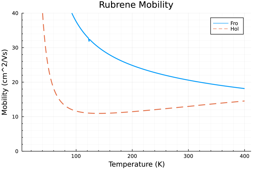
Figure 6: Our predicted mobility of rubrene from the FHIP [2] theory, as a function of temperature (K) for the original Feynman Fröhlich theory (’Fro’) and the Holstein model (’Hol’) we present here.

V Discussion

A major simplification we have made is to lump the Peierls and Holstein electron-phonon contributions together, and then to use these matrix elements in a theory which is designed for the Fröhlich Hamiltonian, and our new theory for the Holstein Hamiltonian. Yam et al. [20] warn that this may be dangerous, as the dispersion in the two models is different.

Perhaps the most surprising aspect of this work is that we have not been able to find any prior attempt to do this, though the mathematical effort was relatively moderate, and the results seem useful. The amount of computational required to produce these plots (optimisation of the variational solution, including numeric quadrature; and numeric quadrature of the influence functional) is trivial compared to the effort of calculating the material properties. Certainly Kornilovitch had mastery of the necessary mathematical machinery two decades ago.

The result is an FHIP mobility theory that seems to have good predictive power, for a range of coupling strengths and underlying polaron quasiparticle character in organic semiconducting crystals. Though the FHIP mobility theory [2] is 60 years old, by extending it with new variational solutions to other forms of electron-phonon coupling, we may find that it continues to be useful in the modelling and design of novel semiconductors.

Further work will be to explore the theory’s predictive power with more applications, including to intrachain mobilities along organic semiconductor polymer backbones.

VI Acknowledgement

B.A.A.M. is supported by an EPSRC Doctoral Training Award. J.M.F. is supported by a Royal Society University Research Fellowship (URF-R1-191292).

Author contributions

The author contributions are defined with the Contributor Roles Taxonomy (CRediT). B.A.A.M.: Investigation, Formal analysis, Methodology, Software, Visualization, Writing – original draft. J.M.F.: Conceptualization, Investigation, Methodology, Software, Supervision, Writing – original draft.

Data access statement

Codes implementing this new Holstein theory are present in our PolaronMobility.jl open-source package[21], along with a script that reproduces the calculations and generates the plots presented here.

References

- Feynman [1955] R. P. Feynman, Slow electrons in a polar crystal, Physical Review 97, 660 (1955).
- Feynman et al. [1962] R. P. Feynman, R. W. Hellwarth, C. K. Iddings, and P. M. Platzman, Mobility of slow electrons in a polar crystal, Physical Review 127, 1004 (1962).
- Fratini et al. [2016] S. Fratini, D. Mayou, and S. Ciuchi, The transient localization scenario for charge transport in crystalline organic materials, Advanced Functional Materials 26, 2292 (2016).
- Giannini et al. [2019] S. Giannini, A. Carof, M. Ellis, H. Yang, O. G. Ziogos, S. Ghosh, and J. Blumberger, Quantum localization and delocalization of charge carriers in organic semiconducting crystals, Nature Communications 10, 10.1038/s41467-019-11775-9 (2019).
- Giannini et al. [2020] S. Giannini, O. G. Ziogos, A. Carof, M. Ellis, and J. Blumberger, Flickering polarons extending over ten nanometres mediate charge transport in high-mobility organic crystals, Advanced Theory and Simulations 3, 2000093 (2020).
- Chang et al. [2022] B. K. Chang, J.-J. Zhou, N.-E. Lee, and M. Bernardi, Intermediate polaronic charge transport in organic crystals from a many-body first-principles approach, npj Computational Materials 8, 10.1038/s41524-022-00742-6 (2022).
- Hellwarth and Biaggio [1999] R. W. Hellwarth and I. Biaggio, Mobility of an electron in a multimode polar lattice, Physical Review B 60, 299 (1999).
- Frost [2017] J. M. Frost, Calculating polaron mobility in halide perovskites, Physical Review B 96, 10.1103/physrevb.96.195202 (2017).
- Osaka [1959] Y. Osaka, Polaron state at a finite temperature, Progress of Theoretical Physics 22, 437 (1959).
- Ordejón et al. [2017] P. Ordejón, D. Boskovic, M. Panhans, and F. Ortmann, Ab initio study of electron-phonon coupling in rubrene, Physical Review B 96, 10.1103/physrevb.96.035202 (2017).
- Kornilovitch and Pike [1997] P. E. Kornilovitch and E. R. Pike, Polaron effective mass from Monte Carlo simulations, Physical Review B 55, R8634 (1997).
- Alexandrov and Kornilovitch [1999] A. S. Alexandrov and P. E. Kornilovitch, Mobile Small Polaron, Physical Review Letters 82, 807 (1999).
- Kornilovitch [2007] P. Kornilovitch, Path integrals in the physics of lattice polarons, arXiv:cond-mat/0702065 103, 192 (2007), arXiv: cond-mat/0702065.
- Coropceanu et al. [2007] V. Coropceanu, J. Cornil, D. A. da Silva Filho, Y. Olivier, R. Silbey, and J.-L. Brédas, Charge transport in organic semiconductors, Chemical Reviews 107, 926 (2007).
- Marcus [1956] R. A. Marcus, On the theory of oxidation-reduction reactions involving electron transfer. i, The Journal of Chemical Physics 24, 966 (1956).
- Nelson et al. [2009] J. Nelson, J. J. Kwiatkowski, J. Kirkpatrick, and J. M. Frost, Modeling charge transport in organic photovoltaic materials, Accounts of Chemical Research 42, 1768 (2009).
- Jortner [1976] J. Jortner, Temperature dependent activation energy for electron transfer between biological molecules, The Journal of Chemical Physics 64, 4860 (1976).
- Kornilovitch [2004] P. E. Kornilovitch, On feynman’s calculation of the froehlich polaron mass (2004).
- Martin and Frost [2022] B. A. A. Martin and J. M. Frost, Multiple phonon modes in feynman path-integral variational polaron mobility (2022), arXiv:2203.16472 .
- Yam et al. [2020] Y.-C. Yam, M. M. Moeller, G. A. Sawatzky, and M. Berciu, Peierls versus holstein models for describing electron-phonon coupling in perovskites, Physical Review B 102, 10.1103/physrevb.102.235145 (2020).
- Frost [2018] J. M. Frost, PolaronMobility.jl: Implementation of the feynman variational polaron model, Journal of Open Source Software 3, 566 (2018).