A time-symmetric soliton dynamics à la de Broglie

Abstract

In this work we develop a time-symmetric soliton theory for quantum particles inspired from works by de Broglie and Bohm. We consider explicitly a non-linear Klein-Gordon theory leading to monopolar oscillating solitons. We show that the theory is able to reproduce the main results of the pilot-wave interpretation for non interacting particles in a external electromagnetic field. In this regime, using the time symmetry of the theory, we are also able to explain quantum entanglement between several solitons and we reproduce the famous pilot-wave nonlocality associated with the de Broglie-Bohm theory.

1 Introduction

Seventy years ago David Bohm Bohm1952 , rediscovering some older results made by de Broglie Valentini ; deBroglie1927 , published his deterministic hidden-variables theory showing that quantum mechanics can be reproduced by a dynamics where particles follow trajectories guided by a $\psi-$wave solution of the Schrödinger equation. This pilot wave theory (PWI) is clearly a counter example against the complacency of the previous period when even the possible existence of hidden variable was contested (e.g., by the von Neumann theorem). Moreover, the PWI is counter-intuitive: It involves a nonlocal ‘spooky’ quantum potential in tension with the theory of relativity, and there is no back-reaction of the particle on the guiding wave (which nature is by the way unclear). For these reasons the proposal made by Bohm is often rejected or criticized. That was the case of Louis de Broglie who actually invented the PWI already in 1926Valentini ; deBroglie1927 but favored a different approach namely the double solution program (DSP) where a particle is a kind of singularity or localized wave (i.e., a soliton) in an oscillating field guiding its motion deBroglie1927 ; deBroglie1956 (for reviews see Fargue ; Fargue2 ; Durt ; Drezet1 ). The DSP was motivated by classical works made by Poincaré, Abraham, Mie Mie1912 , and Einstein to understand particles and waves as merging objects in a deeper (local) field theory. However, due to the constraints imposed by quantum mechanics and Bell’s theorem the DSP was never successfully developed.
In the present work we develop such a theory for a scalar $u-$field solution of a non-linear Klein-Gordon (NLKG) equation involving moving solitons in a external electromagnetic field. As we will see by choosing a specific non-linear term in the NLKG equation, and by using ‘a phase harmony’ condition reminiscent of de Broglie DSP, a self-consistent model can be developed where the soliton core is obeying a dynamics recovering the usual PWI. In our approach the core of the soliton is guided by the phase of the linear Klein-Gordon (LKG) equation. In turn, since the model is completely local, we show that retrocausality associated with waves propagating forward and backward in time is needed in order to reproduce the nonlocal properties of the PWI for several entangled solitons. In the model the nonlocality is thus not fundamental but just effective and results from watching the particle trajectories while ignoring the underlying retrocausal $u-$field that propagates in space-time and guides the solitons. The present work modifies an earlier analysis Submitted in which a nonlocal soliton theory was developed in order to recover the PWI. Moreover, many of the mathematical results derived in Submitted are still valid and used in the present work.

2 The soliton model and its near-field

We start Submitted with the Lagrangian density $\mathcal{L}=Du(x)D^{\ast}u^{\ast}(x)-U(u^{\ast}(x)u(x))$ for a scalar complex field $u(x)\in\mathbb{C}$ with $x:=[t,\mathbf{x}]\in\mathbb{R}^{4}$, and with $D=\partial+ieA(x)$ ($A(x):=[V(x),\mathbf{A}(x)]$ is the electromagnetic potential four-vector and $e$ an electric charge). The nonlinear function $U(y)$ leads to the (Euler-Lagrange) NLKG equation:

$$D^{2}u(x)=-N(u^{\ast}(x)u(x))u(x)$$ (1)

with $N(y):=\frac{dU(y)}{dy}$. This wave equation is different from the linear Klein-Gordon (LKG) equation

$$D^{2}\Psi(x)=-\omega_{0}^{2}\Psi(x)$$ (2)

where $\Psi(x)$ is the standard quantum (relativistic) wavefuntion for a particle of mass $\omega_{0}$.
Next, we use the Madelung/de Broglie representation $u(x)=f(x)e^{i\varphi(x)}$, with $f(x),\varphi(x)\in\mathbb{R}$, in Eq. 1 and obtain a pair of coupled hydrodynamic equations:

$$(\partial\varphi(x)+eA(x))^{2}=N(f^{2}(x))+\frac{\Box f(x)}{f(x)}:=\mathcal{M}^{2}_{u}(x)$$ (3a)

$$\partial[f^{2}(x)(\partial\varphi(x)+eA(x))]=0.$$ (3b)

Moreover, for the LKG equation we write similarly $\Psi(x)=a(x)e^{iS(x)}$, with $a(x),S(x)\in\mathbb{R}$, yielding the pair of coupled hydrodynamic equations:

$$(\partial S(x)+eA(x))^{2}=\omega_{0}^{2}+Q_{\Psi}(x):=\mathcal{M}^{2}_{\Psi}(x)$$ (4a)

$$\partial[a^{2}(x)(\partial S(x)+eA(x))]=0,$$ (4b)

with $Q_{\Psi}(x)=\frac{\Box a(x)}{a(x)}$ the so called quantum potential Bohm1952 ; deBroglie1956 . Here we consider only the cases $\mathcal{M}^{2}_{\Psi}(x)>0$ avoiding tachyonic trajectories. In the following we show how these equations are solved in the vicinity of the soliton core associated with the localized particle.
More precisely, assuming that such a soliton exists as a solution of Eq. 1 or Eq. 3 we write $z(\tau)$ the trajectory of the soliton center labeled by the proper time $\tau$. Associated with this particle motion we define a local Lorentz (proper) rest-frame $\mathcal{R}_{\tau}$ and an hyperplane $\Sigma(\tau)$ with normal direction given by the velocity $\dot{z}(\tau)$. From geometrical considerations a point $x$ belonging to $\Sigma(\tau)$ satisfies the constraint

$$\xi_{\mu}\dot{z}^{\mu}(\tau):=\xi\dot{z}(\tau)=0$$ (5)

with $\xi=x-z(\tau)$ (in $\mathcal{R}_{\tau}$ we have $\xi:=[0,\boldsymbol{\xi}]$) (see Fig. 1). As we showed in Submitted for points $x\in\Sigma(\tau)$ near $z(\tau)$ we can define univocally the structure of the soliton using the variable $\boldsymbol{\xi}$ in $\mathcal{R}_{\tau}$ if $1\gg|\textbf{a}|\cdot|\boldsymbol{\xi}|$ where a is the instantaneous acceleration of the center in the rest-frame $\mathcal{R}_{\tau}$ (i.e., $\xi\ddot{z}\ll 1$). This is interpreted as a condition for defining the notion of quasi-rigidity of the soliton in a relativistic context.

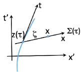
Figure 1: The soliton center trajectory $z(\tau)$ (blue curve) seen from the laboratory reference-frame $t^{\prime},\mathbf{x}^{\prime}$. $\Sigma(\tau)$ is the hyperplane defined by the velocity $\dot{z}(\tau)$ (i.e., any point $x$ belonging to $\Sigma(\tau)$ is such that $\xi=x-z(\tau)$ is normal to $\dot{z}(\tau)$). The time axis $t$ (defined by $\dot{z}(\tau)$) is tangent to the trajectory at the point $z(\tau)$. In this tangent reference frame $\mathcal{R}_{\tau}$ we write $x:=[t,\mathbf{x}]$ and a point belonging to the hyperplane $\Sigma(\tau)$ has coordinates $x=[0,\mathbf{x}]$ whereas $z(\tau):=[0,0]$ and thus $\xi:=[0,\mathbf{x}]$.

Assuming this condition of rigidity is fulfilled we now introduce the so-called ‘phase-harmony condition’ inspired from de Broglie’s DSP deBroglie1927 ; deBroglie1956 :

To every regular solution $\Psi(x)=a(x)e^{iS(x)}$ of Eq. 2 corresponds a localized solution $u(x)=f(x)e^{i\varphi(x)}$ of Eq. 1 having locally the same phase $\varphi(x)\simeq S(x)$, but with an amplitude $f(x)$ involving a generally moving soliton centered on the path $z(\tau)$ and which is representing the particle.

As in Submitted (inspired by some earlier non-relativistic results by Petiau Petiau1954a ; Petiau1954b ; Petiau1955 and others Birula ; Rybakov ) we here write for points $x\in\Sigma(\tau)$ near $z(\tau)$:

$$\varphi(x)\simeq S(z(\tau))-eA(z(\tau))\xi+B(z(\tau))\frac{\xi^{2}}{2}+O(\xi^{3})$$ (6)

which defines the phase-harmony condition up to the second-order approximation in power of $\xi$. The scalar function $B(z(\tau)):=B(\tau)$ is a collective coordinate required in order to consider the deformation of the soliton with time $\tau$. We mention Submitted that Eq. 6 is not gauge invariant and presupposes the Coulomb-Gauge constraint $\boldsymbol{\nabla}\cdot\mathbf{A}=0$ in the local rest frame $\mathcal{R}_{\tau}$. Moreover, the full theory is naturally gauge invariant.
With these properties we can extract from Eq. 3 several important results derived in Submitted . First, if we define $v_{u}(x)$, and $v_{\Psi}(x)$ the velocity of the NLKG and LKG equations respectively

$$v_{u}(x)=-\frac{\partial\varphi(x)+eA(x)}{\mathcal{M}_{u}(x)}$$ (7a)

$$v_{\Psi}(x)=-\frac{\partial S(x)+eA(x)}{\mathcal{M}_{\Psi}(x)}$$ (7b)

we have along $\Sigma(\tau)$

$$v_{u}(x)\simeq v_{\Psi}(z(\tau))+O(\xi),$$ (8a)

$$\mathcal{M}_{u}(x)\simeq\mathcal{M}_{\Psi}(z(\tau))+O(\xi).$$ (8b)

Moreover, by definition we suppose $v_{u}(z(\tau))=\dot{z}(\tau)$ and therefore we obtain here a guidance condition

$$v_{u}(z(\tau))=\dot{z}(\tau)=v_{\Psi}(z(\tau))$$ (9)

as postulated in the original DSP of de Broglie. The phase-harmony condition that we postulate is thus imposing $\partial\varphi(z(\tau))=\partial S(z(\tau))$. The two phase waves $\varphi$ and $S$ are thus connected along the curve $z(\tau)$. Yet, we emphasize that we don’t here impose the second-order matching $\partial_{\mu,\nu}^{2}\varphi(z(\tau))=\partial_{\mu,\nu}^{2}S(z(\tau))$ but only a first-order contact Submitted meaning that $\partial_{\mu,\nu}^{2}\varphi(z(\tau))$ and $\partial_{\mu,\nu}^{2}S(z(\tau))$ are in general different. The relation $\dot{z}(\tau)=v_{\Psi}(z(\tau))$ is actually the definition given to the particle velocity in the PWI fixing a first order dynamical law. In this PWI we directly deduce a second order dynamical law Submitted :

$$\frac{d}{d\tau}[\mathcal{M}_{\Psi}(z(\tau))\dot{z}^{\mu}(\tau)]=\partial^{\mu}[\mathcal{M}_{\Psi}(z(\tau))]+eF^{\mu\nu}(z(\tau))\dot{z}_{\nu}(\tau)$$ (10)

with $F^{\mu\nu}(x)=\partial^{\mu}A^{\nu}(x)-\partial^{\nu}A^{\mu}(x)$ the Maxwell tensor field at point $x:=z$. Moreover, we also deduce in the vicinity of $z(\tau)$:

$$v_{u}(x)\partial\ln{[f^{2}(x)]}+\frac{d}{d\tau}\ln{[\mathcal{M}_{\Psi}(\tau)]}=\frac{3B(\tau)}{\mathcal{M}_{\Psi}(\tau)}+O(\xi)$$ (11)

where we have used the Lagrangian derivative $\frac{d}{d\tau}:=v_{\Psi}(z)\partial_{z}$ for the $\Psi-$field along the particle trajectory $z(\tau)$. From Eq. 11 we deduce

$$\frac{d}{d\tau}\ln{[f^{2}(z(\tau))\mathcal{M}_{\Psi}(\tau)]}=\frac{3B(\tau)}{\mathcal{M}_{\Psi}(\tau)}.$$ (12)

To physically interpret Eq. 12 it is interesting to note that from Eq. 3b we have $v_{u}\partial\ln{(f^{2}\mathcal{M}_{u})}:=\frac{d}{d\tau}\ln{(f^{2}\mathcal{M}_{u})}=-\partial v_{u}$ and that from relativistic hydrodynamics we can define an elementary comoving 3D fluid volume $\delta^{3}\sigma_{0}$ (defined in $\mathcal{R}_{\tau}$) driven by the fluid motion and such that $v_{u}\partial\ln{(\delta^{3}\sigma_{0})}:=\frac{d}{d\tau}\ln{(\delta^{3}\sigma_{0})}=+\partial v_{u}$. Regrouping all these conditions and using $\mathcal{M}_{\Psi}(\tau)=\mathcal{M}_{u}(\tau)$ we obtain

$$-\partial v_{u}(z(\tau))=-\frac{d}{d\tau}\ln{[\delta^{3}\sigma_{0}(z(\tau))]}=\frac{3B(\tau)}{\mathcal{M}_{\Psi}(\tau)}=\frac{d}{d\tau}\ln{[f^{2}(z(\tau))\mathcal{M}_{\Psi}(\tau)]}$$ (13)

which shows that a non-vanishing value for $B(\tau)$ involves a compressibility and ‘deformability’ of the soliton droplet.
A final important equation can be derived in the limit $\xi\ddot{z}\ll 1$ where we have $|\partial_{t}^{2}f|\ll|\boldsymbol{\nabla}^{2}f|$ in the rest-frame $\mathcal{R}_{\tau}$. We obtain Submitted the partial differential equation for the soliton profile for points $x$ belonging to $\Sigma(\tau)$ and localized near $z(\tau)$:

$$[\omega_{0}^{2}+Q_{\Psi}(z(\tau))]f(x)+\boldsymbol{\nabla}^{2}f(x)\simeq N(f^{2}(x))f(x)$$ (14)

with $\boldsymbol{\nabla}:=\frac{\partial}{\partial\boldsymbol{\xi}}$. Moreover, we suppose the soliton core size $r_{0}$ to be much smaller than the Compton wavelength $\omega_{0}^{-1}$ or even $\mathcal{M}_{\Psi}^{-1}$ and therefore in the near-field we have

$$\boldsymbol{\nabla}^{2}f(x)\simeq N(f^{2}(x))f(x).$$ (15)

In Submitted we showed that it is not in general possible to satisfy simultaneously Eq. 15 and Eq. 13 because the condition of existence of an underformable localized wave contradicts Eq. 13. More precisely, assuming a undeformable solution of Eq. 15 we have $f(z(\tau))=f_{0}=Const.$ $\forall\tau$, i.e., from Eq. 13 $B(\tau)=\frac{1}{3}\frac{d}{d\tau}\mathcal{M}_{\Psi}(\tau)$. But since the soliton is undeformable we have also $-\partial v_{u}(z(\tau))=-\frac{d}{d\tau}\ln{[\delta^{3}\sigma_{0}(z(\tau))]}=0$ and therefore $B(\tau)=0$. This implies $\mathcal{M}_{\Psi}(\tau)=Const.$ along the trajectory $z(\tau)$ and contradicts the PWI (where the quantum potential is in general not a constant of motion).
Furthermore, in Submitted we also showed from a version of the Ehrenfest theorem adapted to our nonlinear wave equation that the existence of very small soliton with fastly decaying amplitude with the distance $|\boldsymbol{\xi}|$ generally contradicts the PWI unless $\mathcal{M}_{\Psi}(\tau)=Const.$ along the trajectory $z(\tau)$. In other words, a strongly localized soliton obeys a classical dynamics characterized by a constant mass $\mathcal{M}_{\Psi}(\tau)=Const.$ and don’t reproduce quantum mechanics.
In order to circumvent these objections against the DSP we need here to relax our constraints and we must define a nonlinear function $N(uu^{\ast})$ such that the NLKG equation i) admit a soliton deformable along the trajectory $z(\tau)$, and ii) that the soliton is not too strongly localized in order to avoid the conclusion of Ehrenfest theorem.
For this purpose we here consider a power-law non-linearity (also called Lane-Emden non linearity in the context of astrophysics for modeling stellar structures Chandra ) $N(y)=-\gamma y^{p}$ with $\gamma>0$ and $p\in\mathbb{R}$ an index. Here, we use specifically $p=2$ which leads to a nontrivial but simple solution that was also obtained by G. Mie in his nonlinear electrodynamics involving solitons Mie1912 (see also Rosen1965 ; Schwinger ). The choice $p=2$ has many remarkable properties that can be exploited in the context of the DSP. Writing

$$U(f^{2})=-\frac{r_{0}^{2}}{(\frac{g}{4\pi})^{4}}f^{6}$$ (16a)

$$N(f^{2})=-\frac{3r_{0}^{2}}{(\frac{g}{4\pi})^{4}}f^{4}$$ (16b)

we have in the near field (i.e., Eq. 15 with $\mathcal{M}_{\Psi}(z(\tau))r_{0}(\tau)\ll 1$)

$$\boldsymbol{\nabla}^{2}f(\textbf{x})=-\frac{3r_{0}^{2}}{(\frac{g}{4\pi})^{4}}f^{5}(\textbf{x}).$$ (17)

which admits the radial (non topological) soliton

$$f(\textbf{x}):=F(r)=\frac{g}{4\pi}\frac{1}{\sqrt{r^{2}+r_{0}^{2}}}$$ (18)

(with $r=|\textbf{x}|$) as it can be checked by direct substitution. Eq. 18 has the asymptotic monopolar limit $F(r)\simeq\frac{g}{4\pi}\frac{1}{r}$ if $r\gg r_{0}$ and $F(0)=\frac{g}{4\pi r_{0}}$. $g$ is thus interpreted as a soliton charge (satisfying the integral condition $-\int d^{3}\textbf{x}N(f^{2})f=g$ as shown in Appendix A) while $r_{0}$ acts as a typical radius for the soliton structure. The static energy of the soliton is (see Appendix A) $E_{s}=\frac{g^{2}}{32r_{0}}$.
The non-linearity Eq. 16b is particularly interesting in the context of the DSP since with Eq. 18 it actually vanishes asymptotically for $r\gg r_{0}$, i.e., $N(f^{2})f=-\frac{3g}{4\pi}\frac{r_{0}^{2}}{(r^{2}+r_{0}^{2})^{\frac{5}{2}}}\rightarrow-\frac{3g}{4\pi}\frac{r_{0}^{2}}{r^{5}}$. Far-away of the soliton core the monopolar approximation is thus very good and in this limit it is justified to use instead Poisson’s equation $\boldsymbol{\nabla}^{2}f(\textbf{x})=-g\delta^{3}(\textbf{x})$ for a point-like source. More generally, it is visible that with Eq. 16 the NLKG equation reduces to $\Box u(x)\simeq 0$ if the amplitude of $u\rightarrow 0$. It is important to observe that the asymptotic field $u\propto 1/r$ decays too slowly for applying Ehrenfest theorem (we proved this results in Submitted ). Therefore we evade the conclusions discussed before for a strongly localized droplet.
Eq. 17 possesses an interesting dilation invariance . Indeed, it can directly checked that if $f(\mathbf{x})$ is a solution of Eq. 17 so is the function $\widetilde{f}(\mathbf{x})=\sqrt{\alpha}f(\alpha\mathbf{x})$ where $\alpha\in\mathbb{R}$. In other words, from Eq. 18:

$$\widetilde{f}(\mathbf{x})=\widetilde{F}(r)=\frac{\sqrt{\alpha}g}{4\pi}\frac{1}{\sqrt{\alpha^{2}r^{2}+r_{0}^{2}}}=\frac{g}{4\pi\sqrt{\alpha}}\frac{1}{\sqrt{r^{2}+\frac{r_{0}^{2}}{\alpha^{2}}}}$$ (19)

The second expression shows that the new soliton corresponds to a particle with a new characteristic radius $\tilde{r_{0}}=\frac{r_{0}}{\alpha}$ and a new charge $\tilde{g}=\frac{g}{\sqrt{\alpha}}$ ($-\int d^{3}\textbf{x}N(\widetilde{f}^{2})\widetilde{f}=\tilde{g}$), and Eq. 17 can alternatively be written as

$$\frac{d^{2}}{dr^{2}}\widetilde{F}(r)+\frac{2}{r}\frac{d}{dr}\widetilde{F}(r)+\frac{3\widetilde{r_{0}}^{2}}{(\frac{\widetilde{g}}{4\pi})^{4}}\widetilde{F}^{5}(r)=0$$ (20)

with $r_{0}^{2}/g^{4}=\tilde{r_{0}}^{2}/\tilde{g}^{4}$. Furthermore, observe that the quasi-static energy is invariant, i.e. $\widetilde{E}_{s}=\frac{\tilde{g}^{2}}{32\tilde{r_{0}}}=E_{s}$ during this transformation. Moreover, if $r\gg\tilde{r_{0}}$ we have the asymptotic field

$$\widetilde{F}(r)\simeq\frac{g}{4\pi\sqrt{\alpha}}\frac{1}{r}=\frac{\tilde{g}}{4\pi}\frac{1}{r}$$ (21)

which again confirms that we have a monopolar quasi-static term corresponding to a charge $\tilde{g}$.
Physically, the parameter $\alpha$ can be interpreted as a new collective coordinate for the soliton. More precisely, we now assume that during its motion the soliton typical extension $r_{0}(\tau)$ changes with time $\tau$. We thus write

$$r_{0}(\tau):=\tilde{r_{0}}=r_{0}(0)/\alpha(\tau), g(\tau):=\tilde{g}=\frac{g(0)}{\sqrt{\alpha(\tau)}}$$ (22)

where $\alpha(\tau)$ defines the dynamics concerning the radius. Therefore, for points located not too far from the soliton center Eq.21 generally describes the field along the hyperplane $\Sigma(\tau)$ of Fig. 1. In particular, in the near-field the description is supposed to be very robust because of the condition $\mathcal{M}_{\Psi}(z(\tau))r_{0}(\tau)\ll 1$. We thus write in the near-field defined in the proper rest frame $\mathcal{R}_{\tau}$:

$$F_{\tau}(r):=\widetilde{F}(r)=\frac{\sqrt{\alpha(\tau)}g(0)}{4\pi}\frac{1}{\sqrt{\alpha(\tau)^{2}r^{2}+r_{0}(0)^{2}}}$$

(23)

where the parameter $\alpha(\tau)$ now describes the compressibility or ‘deformability’ of the moving soliton droplet defined along the hyperplane $\Sigma(\tau)$.
The picture obtained is thus the one of a deformable or compressing moving soliton. It is important to see that $B(\tau)$ and $\alpha(\tau)$ can easily be connected. More precisely, writing the local conservation law $\frac{d}{d\tau}\log{[f^{2}(z(\tau))\mathcal{M}_{\Psi}(\tau)\delta^{3}\sigma_{0}(\tau)]}=0$ for a fluid element located at the soliton center we have by integration

$$f^{2}(z(\tau))\mathcal{M}_{\Psi}(\tau)\delta^{3}\sigma_{0}(\tau)=f^{2}(z(0))\mathcal{M}_{\Psi}(0)\delta^{3}\sigma_{0}(0)$$

(24)

Furthermore, from Eq. 23 $f(z(\tau))=F_{\tau}(0)=\sqrt{\alpha(\tau)}F_{0}(0)=\sqrt{\alpha(\tau)}f(z(0)$ and $\delta^{3}\sigma_{0}(\tau)=\frac{1}{\alpha^{3}(\tau)}\delta^{3}\sigma_{0}(\tau)$ (a more rigorous justification is given in Appendix C). Therefore, Eq. 24 leads to

$$\alpha(\tau)=\sqrt{\frac{\mathcal{M}_{\Psi}(\tau)}{\mathcal{M}_{\Psi}(0)}}.$$ (25)

Moreover, we also have $\partial v_{u}(z(\tau))=\frac{d}{d\tau}\log{(\delta^{3}\sigma_{0}(\tau))}=\frac{d}{d\tau}\log{(\alpha^{-3}(\tau))}=-\frac{3}{2}\frac{d}{d\tau}\log{(\mathcal{M}_{\Psi}(\tau))}$ yielding:

$$B(\tau)=\frac{1}{2}\frac{d}{d\tau}\mathcal{M}_{\Psi}(\tau).$$ (26)

Together Eqs. 25 and 26 define the complete deformation/compression of the soliton near-field. In particular, in the non-relativistic regime where the mass $\mathcal{M}_{\Psi}(\tau)$ is approximately constant we have $\alpha(\tau)\simeq 1$ et $B(\tau)\simeq 0$, i.e., $\partial v_{u}(z(\tau))\simeq 0$. We thus recover the picture of an incompressible soliton. In the general relativistic case we get by integration of Eq. 12 and the value of $B(\tau)$ the relation

$$f(z(\tau))=\left(\frac{\mathcal{M}_{\Psi}(\tau)}{\mathcal{M}_{\Psi}(0)}\right)^{1/4}f(z(0))$$ (27)

in agreement with $f(z(\tau))=\sqrt{\alpha(\tau)}f(z(0)$ and Eq. 25.
In the end we thus succeded in obtaining a description of a moving soliton with near-field

$$u(x)=F_{\tau}(r)e^{i\varphi(x)}$$ (28)

with $x\in\Sigma(\tau)$ and where $F_{\tau}$ is given by Eq. 23, $\varphi$ by Eq. 6 (phase harmony condition), and the constraints for $\alpha(\tau)$ and $B(\tau)$ are given by Eqs. 25, 26. The dynamics of the soliton core $z(\tau)$ is piloted by the guidance formula Eq. 9 and recovers the PWI (e.g., Eq. 10).

3 The Time-symmetric de Broglie double solution in the far-field

The previous theory developed for the near-field can be used to define the mide-field and far-field of the soliton. We go back to Eq. 3a written as Eq. 14 and dont neglect the mass term $\mathcal{M}_{\psi}(z(\tau)$. We consider first the case of an uniform motion where $\mathcal{M}_{\Psi}=Const.=\omega_{0}$ and search for a spherical solution of

$$\frac{d^{2}}{dr^{2}}F(r)+\frac{2}{r}\frac{d}{dr}F(r)+\frac{3r_{0}^{2}}{(\frac{g}{4\pi})^{4}}F^{5}(r)+\mathcal{M}_{\Psi}F(r)=0.$$ (29)

In the near-field (i.e., $\mathcal{M}_{\Psi}r\ll 1$) we have Eq. 18 with asymptotic monopolar limit $F(r)\simeq\frac{g}{4\pi}\frac{1}{r}$. In the far-field (i.e., $\mathcal{M}_{\Psi}r\gg 1$) we have $\frac{d^{2}}{dr^{2}}F(r)+\mathcal{M}_{\Psi}F(r)\simeq 0$ which admits the monopole solution: $F(r)\sim\frac{g}{4\pi}\frac{\cos{(\mathcal{M}_{\Psi}(z(\tau))r)}}{r}$. We can easily interpolate these two solutions by writing a solution of Eq. 29 as $F(r)=\frac{g}{4\pi}\frac{G(r/r_{0})}{r}\cos{(\mathcal{M}_{\Psi}r)}$ we obtain for $G(x)$ the differential equation

$$\ddot{G}(x)+\frac{3G^{5}(x)}{x^{4}}\cos{(\mathcal{M}_{\Psi}r_{0})}-2\mathcal{M}_{\Psi}r_{0}\tan{(\mathcal{M}_{\Psi}r_{0})}\dot{G}(x)=0.$$ (30)

After assuming $\mathcal{M}_{\Psi}(z(\tau))r_{0}\ll 1$ (i.e., a very small soliton) it reduces to $\ddot{G}(x)+\frac{3G^{5}(x)}{x^{4}}=0$ which admits the solution $G(x)=\frac{x}{\sqrt{1+x^{2}}}$, i.e.,

$$F(r)\simeq\frac{g}{4\pi}\frac{\cos{(\mathcal{M}_{\Psi}r)}}{\sqrt{r^{2}+r_{0}^{2}}}$$ (31)

which is indeed an interpolation

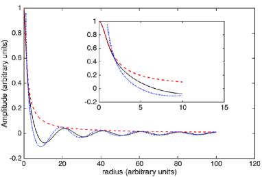
Figure 2: Soliton profile $F(r)$ as a function of the radius $r$. The black curve shows the solution $F(r)$ of the equation $\Delta F=-3F^{5}-AF$ with $A=0.1$. The red dashed curve corresponds to the case $A=0$ (i.e., the Lane-Emden soliton $F(r)=\frac{1}{\sqrt{r^{2}+1}}$). The solutions are obtained numerically by imposing $F(0)=1$ and $\frac{d}{dr}F(0)=0$. The blue dooted curve corresponds to the asymptotic stationary monopole field $F(r)=\frac{\cos{(\sqrt{A}r)}}{r}$. The inset in the right upper corner of the figure is a zoom of the three curves near the soliton center.

between the monopolar and the Lane-Emden quasi-static solutions (see Fig. 2 for a numerical calculation). We check that $-\int d^{3}\textbf{x}N(F^{2})F=g+gO((\mathcal{M}_{\Psi}r_{0})^{2})\simeq g$.
We stress that already in 1925 deBroglie1925a ; deBroglie1925b de Broglie using the linear d’Alembert equation $\Box u(x)=0$ developed a preliminary version of the DSP admitting the monopolar singular field

$$u(t,r)=\frac{g}{4\pi}e^{-i\omega_{0}t}\frac{\cos{(\omega_{0}r)}}{r}.$$ (32)

This $u-$field for a free particle in uniform motion is seen in the Lorentz-reference frame where the particle is at rest at the origin. Eq. 32 is actually a singular solution of the inhomogeneous d’Alembert equation $\Box u(t,\textbf{x})=g\delta^{3}(\textbf{x})e^{-i\omega_{0}t}$ and merges with the far-field of our soliton Eq. 31 and $u=F(r)e^{-i\omega_{0}t}$ if $\omega_{0}:=\mathcal{M}_{\Psi}$.
We stress that Eq. 32 reads $gG^{(0)}_{sym,\omega_{0}}(r)e^{-i\omega_{0}t}$ where

$$G^{(0)}_{sym,\omega}(R)=\frac{\cos{(\omega R)}}{4\pi R}=\frac{1}{2}[\frac{e^{i\omega R}}{4\pi R}+\frac{e^{-i\omega R}}{4\pi R}]$$ (33)

($R=|\mathbf{x}-\mathbf{x}^{\prime}|$) is the time-symmetric Green function of the Helmholtz equation: $[\omega^{2}+\boldsymbol{\nabla}^{2}]G^{(0)}_{\omega}(R)=-\delta^{3}(\mathbf{x}-\mathbf{x}^{\prime})$. In other words, $u(t,r)$ in Eq. 32 is a time-symmetric solution $u=\frac{1}{2}(u_{ret}+u_{adv})$ of $\Box u(t,\textbf{x})=g\delta^{3}(\textbf{x})e^{-i\omega_{0}t}$. This is fundamental because it leads to the stability of the micro-object: The energy radiation losses associated with the retarded wave are exactly compensated by the energy flow associated with the converging advanced wave. Furthermore, it implies a time-symmetric causality which is reminiscent of early ideas by Tetrode and Page Tetrode ; Page for explaining the stability of atomic orbits. Such ideas were later resurrected by Fokker Fokker , Feynman and Wheeler in their absorber theory WF , and by Hoyle and Narlikar for cosmological models involving a time-symmetric creation-field Hoyle . Interestingly, this idea involving time-symmetry was also discussed in 1925 by de Broglie deBroglie1925a ; deBroglie1925b but was soon abandoned by him and he never came back to this suggestion (even after his collaborator Costa de Beauregard developped a retrocausal interpretation of the EPR paradox Beauregard ).

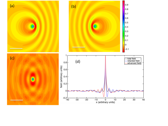
Figure 3: Soliton profile $\textrm{Re}[u(x,y,z=0,t=0)]$ for a particle in uniform motion (velocity $v_{x}=0.6$ along the $x$ direction) in the laboratory frame. (a) and (b) are respectively the advanced and retarded fields contributions $\textrm{Re}[u_{ret./adv.}(x,y,z=0,t=0)]$, and (c) is the whole time-symmetric field $\textrm{Re}[u_{sym}(x,y,z=0,t=0)]=\frac{1}{2}\textrm{Re}[u_{ret.}(x,y,z=0,t=0)+u_{adv.}(x,y,z=0,t=0)]$. (d) shows a crosscut along the x direction of the three fields $\textrm{Re}[u_{ret.}(x,y=0,z=0,t=0)]$ (red curve), $\textrm{Re}[u_{adv.}(x,y=0,z=0,t=0)]$ (blue curve), and $\textrm{Re}[u_{sym.}(x,y=0,z=0,t=0)]$ (black curve). For the present calculations we used $\omega_{0}\gamma=1$ and $a=\frac{1}{\sqrt{10}}\gamma\simeq 0.3953$ in Eqs. 34, 35. The scale bar used in (a-c) is 10 units long.

To appreciate the time-symmetric nature of our soliton we represent in Fig. 3 $\textrm{Re}[u(x,y,z=0,t=0)]$ in the laboratory frame where the soliton moves at the velocity $v_{x}$ along the $+x$ direction. Using Eq. 31 for the interpolated solution we have

$$\textrm{Re}[u(\mathbf{x},t)]\simeq\frac{g}{4\pi}\frac{\cos{(\omega_{0}R)}cos{[\omega_{0}\gamma(t-v_{x}x)}]}{\sqrt{r_{0}^{2}+R^{2}}}$$ (34)

with $R=\sqrt{(x-v_{x}t)^{2}\gamma^{2}+y^{2}+z^{2}}$ and $\gamma=(1-v_{x}^{2})^{-\frac{1}{2}}$. Moreover, writing $u:=u_{sym}=\frac{1}{2}[u_{adv.}+u_{ret.}]$ and still using the interpolated field we can define

$$\textrm{Re}[u_{ret./adv.}(\mathbf{x},t)]\simeq\frac{g}{4\pi}\frac{\cos{[\omega_{0}\gamma(t-v_{x}x)\mp\omega_{0}R]}}{\sqrt{r_{0}^{2}+R^{2}}}$$ (35)

associated with propagating diverging/converging waves. Comparing Eqs. 35 and 34 shows that the particle core is surfing a wave front reminiscent of what is occurring with a airplane in the subsonic regime (with here the velocity of light replacing the velocity of sound). The wave front precedes the particle in the retarded case and follows the particle in the advanced case. The superposition $\textrm{Re}[u_{sym.}(x,y,z=0,t=0)$ induces a phase wave $cos{[\omega_{0}\gamma(t-v_{x}x)}]$ associated with de Broglie’s guiding field (i.e., the guiding wave involved in the PWI).

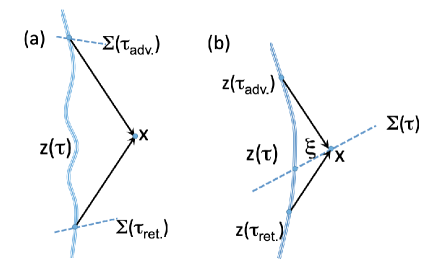
Figure 4: (a) Far-field of the soliton $u(x)$ at point $x$ away from the ‘singularity’ trajectory $z(\tau)$. The field is emitted at retarded/advanced (proper) time $\tau_{ret/adv}$. (b) Same as in (a) but in the vicinity of the trajectory $x\sim z$ where we evaluate the field in the hyperplane $\Sigma(\tau)$ at distance $\xi=x-z(\tau)$.

The previous theory for the far-field can be generalized. For this purpose start from Eq. 1 written as $D^{2}u(x)=-N(u^{\ast}(x)u(x))u(x):=J(x)$. Using Green’s theorem a formal solution reads

$$u(x)=\int K(x,y)J(y)d^{4}y+u_{free}(x)$$ (36)

where $u_{free}(x)$ is a solution of the homogeneous equation $D^{2}u(x)=0$, and the propagator $K(x,x^{\prime})$ satisfies $D^{2}K_{sym}(x,x^{\prime})=\delta^{4}(x-x^{\prime})$. Consider first the case $A(x)=0$ (i.e., absence of external field). We see that a natural choice corresponds to $u_{free}(x)=0$ and $K^{(0)}_{sym}(x,x^{\prime})=\frac{K^{(0)}_{ret}(x,x^{\prime})+K^{(0)}_{adv}(x,x^{\prime})}{2}$ where

$$K^{(0)}_{sym}(x,x^{\prime})=\frac{\delta[(x-x^{\prime})^{2})]}{4\pi}=\frac{1}{2}[\frac{\delta(t-t^{\prime}-R)}{4\pi R}+\frac{\delta(t-t^{\prime}+R)}{4\pi R}]$$ (37)

(with $R=|\mathbf{x}-\mathbf{x}^{\prime}|^{2}$) is the time-symmetric propagator.
As shown in Fig. 4(a) the evaluation of the far-field at point $x$ requires the knowledge of the source term $J(x)$ in the vicinity of the trajectory $z(\tau)$ along two hyperplanes $\Sigma(\tau_{ret.})$, $\Sigma(\tau_{adv.})$ associated with retarded and advanced emissions by the particle. These planes are obtained by finding intersections of the trajectory $z(\tau)$ with the backward and forward light cones with common apex located at point $x$. We have approximately:

$$u(x)\simeq\frac{1}{2}\int\int_{\Sigma(\tau_{ret.})}K^{(0)}_{ret}(x,z(\tau_{ret}))J(\tau_{ret},\boldsymbol{\xi})d^{3}\boldsymbol{\xi}d\tau_{ret.}$$

$$+\frac{1}{2}\int\int_{\Sigma(\tau_{adv.})}K^{(0)}_{adv}(x,z(\tau_{adv}))J(\tau_{adv},\boldsymbol{\xi})d^{3}\boldsymbol{\xi}d\tau_{adv.}$$

where the integrations are done in the local rest frame $\mathcal{R}_{\tau_{ret.}}$ and $\mathcal{R}_{\tau_{adv.}}$. After spatial integration over the hyperplanes $\Sigma(\tau_{ret.})$, $\Sigma(\tau_{adv.})$ and using the lowest order approximation $\int_{\Sigma(\tau)}J(\tau,\boldsymbol{\xi})d^{3}\boldsymbol{\xi}=-\int d^{3}\textbf{x}N(F_{\tau}^{2})F_{\tau}e^{iS(z(\tau))}\simeq g(\tau)e^{iS(z(\tau))}=g(0)\frac{e^{iS(z(\tau))}}{\sqrt{\alpha(\tau)}}$ (see Eq. 28 with $\varphi\simeq S$) we obtain for the far-field:

$$u(x)=g(0)\int_{(C)}K^{(0)}_{sym.}(x,z(\tau))\frac{e^{iS(z(\tau))}}{\sqrt{\alpha(\tau)}}d\tau$$ (39)

with $\alpha(\tau)=\sqrt{\frac{\mathcal{M}_{\Psi}(\tau)}{\mathcal{M}_{\Psi}(0)}}$ and the integration is over the whole trajectory $C$. This field is a solution of

$$\Box u(x)=g(0)\int_{(C)}\delta^{4}(x-z(\tau))\frac{e^{iS(z(\tau))}}{\sqrt{\alpha(\tau)}}d\tau$$

$$=g(0)\delta^{3}(\mathbf{x}-\mathbf{z}(t))\frac{e^{iS(t,\mathbf{z}(t))}}{\sqrt{\alpha(\tau)}}\sqrt{1-\mathbf{v}^{2}(t)}$$ (40)

which shows that the coupling vanishes when the velocity of the particle $\mathbf{v}$ approaches the celerity of light.
We stress that using Eq. 28 in $\int_{\Sigma(\tau)}J(\tau,\boldsymbol{\xi})d^{3}\boldsymbol{\xi}$ looks like a physical ansatz. To justify the self-consistency of the ansatz we now explicit Eq. 40 using Eq. 37:

$$u(x)=\frac{1}{2}\left([\frac{g(\tau)e^{iS(z(\tau))}}{4\pi\rho(\tau)}]_{\tau_{ret.}}+[\frac{g(\tau)e^{iS(z(\tau))}}{4\pi\rho(\tau)}]_{\tau_{adv.}}\right)$$ (41)

with $\rho(\tau)=|(x-z(\tau))\cdot\dot{z}(\tau)|$. The derivation of this formula is clearly reminiscent from the Lienard-Wiechert potentials in classical electrodynamics . To justify the ansatz used above the goal is to compute $u(x)$ with Eq. 41 in the vicinity of the trajectory $z(\tau)$ in order to recover the asymptotic near-field $u\propto 1/r$ obtained in Sec. 2. The method has been already developed by Dirac Dirac for the classical electron and requires lengthy calculations that will not be shown here for questions of space. We here summarize the main steps of the methods. As shown in Fig. 4(b) the field is evaluated in the hyperplane $\Sigma(\tau)$ at a distance $r=\sqrt{-\xi^{2}}$ that requires the retarded and advanced fields in Eq. 41 at (proper) times $\tau_{ret}=\tau-\sigma_{-}$ and $\tau_{ret}=\tau+\sigma_{+}$ with $\sigma_{\pm}\sim r$. Using the conditions $(x-z(\tau\mp\sigma_{\mp}))^{2}=0$ for the points on a light cone we deduce after lengthy calculations Dirac the values $\rho_{\mp}=\rho(\tau\mp\sigma_{\mp})$, i.e.:

$$\frac{1}{\rho_{\mp}}=\frac{1}{r}[1+\frac{1}{2}\xi\ddot{z}+\frac{3}{8}(\xi\ddot{z})^{2}\mp\frac{r}{3}\xi z^{(3)}+\frac{5r^{2}(\ddot{z})^{2}}{24}+O(r^{3})]$$ (42)

where the derivatives and $\xi$ are calculated at time $\tau$. The field is thus $u(x)=\frac{u_{-}+u_{+}}{2}$ with $u_{\mp}=\frac{g(\tau\mp\sigma_{\mp})e^{iS(\tau\mp\sigma_{\mp})}}{8\pi\rho_{\mp}}$ that leads to:

$$u(x)=\frac{g(\tau)e^{iS(z(\tau))}}{4\pi r}[1+\frac{\xi\ddot{z}}{2}+\frac{r^{2}}{2}(i\ddot{S}-(\dot{S}-i\frac{\dot{g}}{g})^{2})$$

$$+r^{2}\frac{d^{2}}{d\tau^{2}}\ln{(g)}+\frac{3}{8}(\xi\ddot{z})^{2}+\frac{5}{24}(r\ddot{z})^{2}+O(r^{3})].$$ (43)

for points $x\in\Sigma(\tau)$ at a distance $r$ from $z(\tau)$.
From Eq. 43 we deduce that at the lowest order we have indeed $u(x)\simeq\frac{g(\tau)e^{iS(z(\tau))}}{4\pi r}$ and we recover the asymptotic soliton near-field discussed in Sec. 2. This shows that our ansatz concerning $\int_{\Sigma(\tau)}J(\tau,\boldsymbol{\xi})d^{3}\boldsymbol{\xi}$ is indeed justified. Moreover, in the case of an uniform motion with $\ddot{z}=0$, $\ddot{S}=0$, $\dot{S}=-\omega_{0}$, $\dot{g}=0$, $\ddot{g}=0$ we have $u(x)=\frac{ge^{-i\omega_{0}\tau}}{4\pi r}[1-\frac{\omega_{0}r^{2}}{2}+O(r^{3})]\simeq\frac{ge^{-i\omega_{0}\tau}\cos{(\omega_{0}r)}}{4\pi r}$ that is the field associated with the monopole discussed above.
Furthermore, from Eq. 43 and the definition $u=fe^{i\varphi}$ we compute the ratio $\frac{u(x)}{u^{\ast}(x)}=e^{i2\varphi(x)}$ and obtain

$$\frac{u(x)}{u^{\ast}(x)}=e^{i2\varphi(x)}=e^{i2S}[1+ir^{2}(\ddot{S}+2\frac{\dot{S}\dot{g}}{g})+O(r^{3})].$$ (44)

Comparing this with the Taylor expansion $e^{i2\varphi(x)}=e^{i2\varphi(z)}[1+i2\xi\partial\varphi(z)+O(r^{2})]$ we deduce immediately that the first-order term must vanish

$$\xi\cdot\partial\varphi(z)=0$$ (45)

and since we have also by definition $\xi\dot{z}=0$ we have thus $\dot{z}(\tau)$ parallel (i.e., proportional) to $\partial\varphi(z)$. In other words, since $\dot{z}^{2}=1$, we recover the guidance formula Eq. 9 $\dot{z}(\tau)=-\frac{\partial\varphi(z(\tau))}{\sqrt{(\partial\varphi(z(\tau)))^{2}}}$ (in absence of external field $A(x)$) discussed in Sec. 2 in the near-field. The fact that we can recover this result from Eq. 41 associated with the far-field again confirms the self-consistency of our approach.
In presence of an external field $A(x)\neq 0$ the previous propagator method can be generalized. For this we first replace the partial derivative $\partial$ by the covariant derivative $D=\partial+ieA(x)$ in Eq. 40 leading to

$$D^{2}u(x)=g(0)\int_{(C)}\delta^{4}(x-z(\tau))\frac{e^{iS(z(\tau))}}{\sqrt{\alpha(\tau)}}d\tau$$ (46)

with solution

$$u(x)=g(0)\int_{(C)}K_{sym}(x,z(\tau))\frac{e^{iS(z(\tau))}}{\sqrt{\alpha(\tau)}}d\tau$$ (47)

and $K_{sym}(x,x^{\prime})$ the time-symmetric propagator solution of $D^{2}K_{sym}(x,x^{\prime})=\delta^{4}(x-x^{\prime})$. A formal solution for the propagator reads

$$K_{sym}(x,x^{\prime})=K^{(0)}_{sym}(x,x^{\prime})+K^{(ref)}_{sym}(x,x^{\prime})$$ (48)

where $K^{(ref)}_{sym}(x,x^{\prime})=\int d^{4}yK^{(0)}_{sym.}(x,y)\hat{\mathcal{O}}_{y}K_{sym}(y,x^{\prime})$ (with the operator $\hat{\mathcal{O}}_{y}:=e^{2}A(y)^{2}-ie\partial_{y}A(y)-2ieA(y)\partial_{y}$) defines the reflected part of the propagator resulting from the interaction of the vacuum solution $K^{(0)}_{sym}$ with the potential $A$. Therefore, the $u-$field splits as

$$u(x)=u^{(0)}(x)+u^{(ref)}(x)$$ (49)

where $u^{(0)}(x)$ evaluated using $K^{(0)}_{sym}(x,x^{\prime})$ leads to Eq. 41 and $u^{(ref)}(x)$ is evaluated using $K^{(ref)}_{sym}(x,x^{\prime})$. As we saw the singular field $u^{(0)}(x)$ is diverging as $u(x)\simeq\frac{g(\tau)e^{iS(z(\tau))}}{4\pi r}$ near $x\sim z(\tau)$. The reflected part is in general a much more regular and weaker field near $x\sim z(\tau)$.
Moreover, near the point $x\sim z(\tau)$ we can assume $A(x)\simeq A(z)=const.$ (the soliton is supposed much smaller than the variation of $A$) and we check directly that the function $K_{sym}(x,x^{\prime})=K^{(0)}_{sym}(x,x^{\prime})e^{-ieA(z)(x-x^{\prime})}$ is a solution of $(\partial+ieA(z))^{2}K_{sym}(x,x^{\prime})=\delta^{4}(x-x^{\prime})$. Inserting this result in Eq. 39 where $K_{sym}(x,z(\tau))$ replaces $K^{(0)}_{sym}(x,z(\tau))$ we obtain once more Eq. 41 with the substitution $e^{iS(z(\tau_{ret/adv}))}\rightarrow e^{iS(z(\tau_{ret/adv}))}e^{-ie(x-z(\tau_{ret/adv})A}$. In the vicinity of $z(\tau)$ in the hyperplane $\Sigma(\tau)$ we obtain at the lowest order:

$$\frac{u(x)}{u^{\ast}(x)}=e^{i2S}[1-i2e\xi A(z(\tau))+O(r^{2})]=e^{i2\varphi(z)}[1+i2\xi\partial\varphi(z)+O(r^{2})],$$ (50)

which implies

$$\xi\cdot(\partial\varphi(z)+eA(z))=0.$$ (51)

Therefore, using once more $\xi\dot{z}=0$, we recover the guidance formula Eq. 9, i.e., $\dot{z}(\tau)=-\frac{\partial\varphi(z(\tau))+eA(z(\tau))}{\sqrt{(\partial\varphi(z(\tau))+eA(z(\tau)))^{2}}}$ derived in Sec. 2.
This analysis shows that even if in general $|u^{(0)}(x)|\gg|u^{(ref)}(x)|$ in the vicinity of $x\sim z$ the phase is however globally influenced by the presence of the external field $A(x)$ imposing the guidance formula.

4 Discussion: Entanglement, generalizations, perspectives

In order to conclude this article we would like to emphasize some general properties of our model. First, concerning the methodology we started in Sec. 2 with a near-field approach assuming a field with a spherical symmetry $f=F_{\tau}(r)$ (see Eq. 23). This actually neglects the contribution of the reflected field. The consistency of our model becomes more obvious if we formally write the full $u-$field as $u(x)=u^{(0)}(x)+u^{(ref)}(x)$ with

$$u^{(0/ref)}(x)=-\frac{3r_{0}^{2}}{(\frac{g}{4\pi})^{4}}\int K^{(0/ref)}_{sym}(x,y)(f(y))^{5}e^{i\varphi(y)}d^{4}y$$

$$\simeq-\frac{3r_{0}^{2}}{(\frac{g}{4\pi})^{4}}\int K^{(0/ref)}_{sym}(x,y)(f^{(0)}(y))^{5}e^{i\varphi(y)}d^{4}y$$ (52)

where we used the approximation $f\simeq f^{(0)}$ for evaluating the source term in the second line. This is justified since we assume $f^{(ref)}\ll f^{(0)}$ in the core region of the soliton where the integral contributes. This shows that $u^{(0/ref)}(x)$ are determined by the knowledge of the soliton $f^{(0)}(x)$ in the near-field as assumed in Section. 2. Moreover we could in principle obtain deviations to this approximation. That could occur for regimes where the reflected field is not small, e.g., in very strong (relativistic) fields leading to further non-linearities.
To give an illustration of this issue consider a particle at rest in the middle of a spherical ideal cavity of radius $R$ with a perfectly reflecting wall associated with an infinite potential wall. The far-field stationary spherical solution of the equation $\Box u(t,\textbf{x})=g\delta^{3}(\textbf{x})e^{-i\omega t}$ reads

$$u(t,r)=\frac{ge^{-i\omega t}}{4\pi r}[\cos{(\omega r)}-\textrm{cotan}(\omega R)\sin{(\omega r)}]$$ (53)

and obeys the boundary condition $u(R,t)=0$. Near the origin (where $\omega r<<1$) the reflected field $f^{(ref)}=\textrm{cotan}(\omega R)\frac{g\sin{(\omega r)}}{4\pi r}\simeq-\textrm{cotan}(\omega R)\frac{g\omega}{4\pi}$ is in general much smaller than $f^{(0)}=\frac{g\cos{(\omega r)}}{4\pi r}\simeq\frac{g}{4\pi r}$ unless the ‘cotan’ term is diverging which occurs if $\omega=\frac{m\pi}{R}$ with $m\in\mathbb{N}$. If that happens then the field in the cavity blows up and the approximations $f^{(ref)}\ll f^{(0)}$ breaks down. Moreover, don’t forget that the particle is actually guided by the LKG equation Eq. 2 with spherical eigen-solutions $\Psi_{n}(t,r)=\frac{\sin{(n\pi r/R)}}{r}e^{-i\omega_{n}t}$ with $\omega_{n}=\sqrt{(\omega_{0}^{2}+\frac{n^{2}\pi^{2}}{R^{2}})}\simeq\omega_{0}+\frac{n^{2}\pi^{2}}{2\omega_{0}R^{2}}$ and $n\in\mathbb{N}$. The particle is at rest in agreement with the PWI and we have $\omega=\omega_{n}\simeq\omega_{0}$ in Eq. 53. We see that problem occurs only if $\omega_{0}\simeq\frac{m\pi}{R}$. But this possibility can be rejected for at least two reasons. First, this would imply a strong conspiracy or fine-tuning where the Compton wavelength of the particle $\lambda_{0}=2\pi/\omega_{0}$ matches $2R/m$. This corresponds to very small cavities of the size of the particle and we enter in the QED regime where particle/antiparticle pairs could be created. This regime is not considered in our analysis.

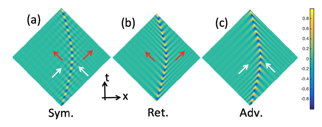
Figure 5: (a) Time-symmetric $u-$field associated with a particle following a curved trajectory in the plane $x-t$ [here we use the hyperbolic trajectory $x(t)=-\sqrt{x_{0}^{2}+v_{0}^{2}t^{2}}$]. (b) and (c) show the retarded and advanced $u-$fields associated wit the same trajectory. The fields are calculated numerically using expressions Eqs. 39,41 and similar ones for retarded/advanced fields. The singularity of these far-fields on the particle are removed by modifying the pole as $\frac{1}{r}\rightarrow\frac{1}{\sqrt{(r^{2}+r_{0}^{2})}}$ with $r_{0}$ a small constant. For simplicity we here used the classical phase $S=-\omega_{0}\tau$ for the particle action with $\tau$ the proper time.

Moreover, the second more physical reason for rejecting this implausible resonance is that in general the potential barrier is not infinite and we can show that if the potential step $|eV|$ is smaller than $\omega_{0}$ the field given by Eq. 53 is modified: There is no strong reflectivity at the boundary $r=R$ and $u^{(0)}$ is mostly unaffected , i.e., $u\simeq u^{(0)}$. Again all this analysis is consistent if the potential is not too strong so that particle/antiparticle pairs are not generated (pairs are potentially generated if $|eV|\simeq 2\omega_{0}$).
An important related problem concerns energy conservation and causality for a particle moving in an external field. Consider a particle following a curved trajectory like the one shown in Fig. 5 and emitting a retarded + advanced field as given in Eqs. 39,41, i.e., neglecting the reflected part for simplicity. As visible on Fig. 5(a) the time-symmetric field implies that waves are constantly radiated into the future and into the past directions. De Broglie in 1957 deBroglie1956 analyzed the problem in terms of retarded waves (as shown in Fig. 5(b)) and concluded that the basic DSP leads to a paradox known as Perrin’s objection (for a discussion see Drezet1 ): Following this objection a particle interacting with an external field, like a beam splitter, should radiate energy in empty branches not followed by the particle. After several interactions of that kind the particle (i.e., the $u-$wave) should have lost all its energy in contradiction with experiments showing that particles are detected with a finite energy (the same issue remains in the double-slit experiment where the potential acting on the particle is mostly of quantum origin). This problem is reminiscent of the interpretation of empty waves in the PWI where their peculiar energetic properties are often seen as a difficulty.
Moreover we now see that the problem disappears in our theory: The energy losses associated with radiated waves (i.e., Fig. 5(b)) are compensated by the energy gain associated with the advanced waves converging on the particle (i.e., Fig. 5(c)). From the point of view of usual causality this looks conspiratorial or superdeterministic. A ‘de Broglie-Bohm demon’ having access to this flow of energy and perceiving the time going from past to future would see a converging flow of energy coming from the remote space arriving precisely at the good time in a coherent way on the particle. Furthermore, a retarded wave is also emitted by the particle and the sum off both waves gives the soliton field discussed in Secs. 2 and 3 imposing the guidance formula. As we showed in Sec. 2 it is possible to build a stationary soliton field in the local rest frame. When merging this near-field with the far-field of Sec. 3 the time-symmetric structure is thus required for consistency. Therefore, in our model the non-linearity of the wave equation and the existence of stable stationary solitons involves a time-symmetric causality. This in turn allows us to preserve energy conservation (more on this is derived in Appendix D) and reproduce the predictions of the PWI, i.e., of quantum mechanics (in the regimes considered here).
The theory discussed in this work focused on the single particle/soliton problem and we showed that a time-symmetric $u-$field is required. This time-symmetric causality is clearly of great importance concerning the problem of entanglement between several particles. As it is well-known in de Broglie Bohm mechanics Hiley non-locality is offered as an explanation for justifying violations of Bell’s inequality. However, the present theory is definitely local and its quantitative predictions should therefore apriori differ from the standard PWI. It is here that the time-symmetry of the model comes to the rescue.
To see how it works, we consider the many-body generalization to an ensemble of $N$ indistinguishable (bosonic) particles of the LKG equation for a single particle developed in Sec. 2. We have the wavefunction $\Psi_{N}(x_{1},...x_{i},...x_{N})$ solution of the set of $N$ coupled equations $D_{i}^{2}\Psi_{N}=-\omega_{0}^{2}\Psi_{N}$ equivalent to the set of hydrodynamic equations:

$$(\partial_{i}S_{N}(X)+eA(x_{i}))^{2}=\omega_{0}^{2}+\frac{\Box_{i}a_{N}(X)}{a_{N}(X)}:=\mathcal{M}^{2}_{\Psi_{N},i}(X)$$ (54a)

$$\partial_{i}[a_{N}^{2}(X)(\partial_{i}S_{N}(X)+eA(x_{i}))]=\partial_{i}[a_{N}^{2}(X)\mathcal{M}_{\Psi_{N},i}(X)v_{\Psi_{N},i}(X)]=0,$$ (54b)

where we introduced the notation $X:=[x_{1},...,x_{N}]$ and the velocity $v_{\Psi_{N},i}(X):=-\frac{\partial_{i}S_{N}(X)+eA(x_{i})}{\mathcal{M}_{\Psi_{N},i}(X)}$ (we also assume $\mathcal{M}^{2}_{\Psi_{N},i}(X)>0$). In the PWI we define the velocity of the $N$ particles through the guidance relations

$$\frac{dz_{i}(\lambda)}{d\tau_{i}}=\frac{\dot{z}_{i}(\lambda)}{\sqrt{\dot{z}_{i}(\lambda)\dot{z}_{i}(\lambda)}}=v_{\Psi_{N},i}(Z(\lambda))$$ (55)

with $Z(\lambda):=[z_{1}(\lambda),...,z_{N}(\lambda)]$, $\dot{z}_{i}(\lambda):=\frac{dz_{i}(\lambda)}{d\lambda}$ and $d\tau_{i}=\sqrt{\dot{z}_{i}(\lambda)\dot{z}_{i}(\lambda)}d\lambda$ is a proper time element along the trajectory of the $i^{th}$ particle. We stress that in this description we require a parameter $\lambda$ to synchronize the $N$ particles. Usually this is done by involving a preferred foliation $\mathcal{F}$ of Minkowski’s space-time with space-like hyperplanes. Choosing $\mathcal{F}$ in general particularizes a set of entangled trajectories defining an ensemble $M(\mathcal{F})$. Moreover, since the choice of $\mathcal{F}$ is arbitrary the PWI admits an infinite number of possible paths-ensemble $M(\mathcal{F})$. Clearly, there is an apparent tension with relativity since the ensemble of trajectories is not unique and depends on a foliation sometimes identified with a kind of ‘Bohmian-Aether’ (for a discussion on this issue see Drezet2019 ). In the context of our relativistic local theory for a $u-$field we don’t here give any ontological content to the particular foliation used $\mathcal{F}_{0}$ to specify the particle trajectories. Instead, it is the (infinite) ensemble of all the $M(\mathcal{F})$ that exhausts the set of possibilities; and the choice $\mathcal{F}_{0}$ used in our Universe (or in the part of our Universe accessible to us and entangled with us) is associated with a particular choice on initial conditions (perhaps related to cosmological constraints Drezet2019 ). We stress that the dynamics Eq. 55 is not in general ‘statistically transparent’, i.e., that it cannot always reproduce Born’s rule and the statistical predictions of quantum mechanics (more on this will published in a subsequent article). Moreover, in the non-relativistic regime or in finite asymptotic regions of space-time, i.e., before or after scattering or interactions with an external field, we can justify Born’s rule and recover statistical transparency.
In the present local theory for the $u-$field the $N$ solitons move in the same 4D space time and not in the abstract configuration space. The far-field for the $N$ entangled soliton is written in analogy with Eq. 47 as:

$$u(x)=\sum_{i}u_{i}(x)=\sum_{i}g(0)\int_{(C_{i})}K_{sym}(x,z_{i}(\lambda))\frac{e^{iS_{N}(Z(\lambda))}}{\sqrt{\alpha_{i}(\lambda)}}d\tau_{i}$$ (56)

with $\alpha_{i}(\lambda)=\sqrt{\frac{\mathcal{M}_{\Psi_{N},i}(Z(\lambda))}{\mathcal{M}_{\Psi,i}(Z(0))}}$. This field obeys the following local equation:

$$D^{2}u(x)=\sum_{i}g(0)\int_{(C_{i})}\delta^{4}(x-z_{i}(\lambda))\frac{e^{iS_{N}(Z(\lambda))}}{\sqrt{\alpha_{i}(\lambda)}}d\tau_{i}$$ (57)

that is defined in the 4D Minkowski spacetime not in the configuration space. This wave equation and dynamics is local but the $N$ singularities moving along the $N$ trajectories $C_{i}$ are clearly entangled through the phase $S_{N}(Z_{i}(\lambda))$ and the masses $\mathcal{M}_{\Psi_{N},i}(Z(\lambda))$ defined in the PWI of Eqs. 54a,54b. The $N$ trajectories are synchronized using the parameter $\lambda$ and a specific foliation $\mathcal{F}$.

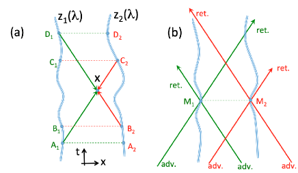
Figure 6: (a) Sketch of $u-$field created at space-time point $x$ by two entangled particles 1 and 2 with trajectories $z_{1}(\lambda),z_{2}(\lambda)$. The retarded field emitted by particle 1 at point $A_{1}$ (forward in time green arrow) depends on the knowledge of the position of the particle 2 located at $A_{2}$. The same is true for the advanced field created at point $D_{1}$ by particle 1 (backward in time green arrow) and depending on the position of particle 2 at $D_{2}$. The situation is the similar for the field created by particle 2 (red arrows) at $B_{2}$ and $C_{2}$ synchronized with the particle 1 at $B_{1}$ and $C_{1}$. (b) The particle 1 at $M_{1}$ and 2 at $M_{2}$ are excited by advanced waves coming from the past and in turn emit retarded waves going into the future. The synchronization and correlation of the two particles are related to the time-symmetric causal connection with information located in the remote past and future.

Consider for example a pair of particles 1 and 2 with entangled trajectories $z_{1}(\lambda),z_{2}(\lambda)$ defined with the PWI guidance formula Eq. 55. The $u-$field at point $x$ is the sum of the contributions $u_{1}(x)$ and $u_{2}(x)$ generated by the particle $1$ and $2$ respectively. In the example of Fig. 6(a) (i.e., in absence of external $A-$field) $u_{1}(x)$ splits into a retarded contribution emitted from the particle $1$ when it was at $A_{1}=[t_{A_{1}},\mathbf{x}_{A_{1}}]$ and an advanced contribution emitted from the same particle when it was at $D_{1}=[t_{D_{1}},\mathbf{x}_{D_{1}}]$. Moreover, when the particle $1$ is at $A_{1}$ ($D_{1}$) the second particle is at point $A_{2}$ ($D_{2}$) as determined by the preferred foliation $\mathcal{F}$ (here we consider the set of hyperplanes $t=const.$ for such a foliation). We can use Eq. 41 to evaluate $u_{1}$:

$$u_{1}(x)=\frac{g(0)}{2}\left([\frac{e^{iS(z_{1}(\lambda),z_{2}(\lambda))}}{4\pi\sqrt{\alpha_{1}(\lambda)}\rho_{1}(\lambda)}]_{\lambda=t_{A_{1}}}+[\frac{e^{iS(z_{1}(\lambda),z_{2}(\lambda))}}{4\pi\sqrt{\alpha_{1}(\lambda)}\rho_{1}(\lambda)}]_{\lambda=t_{D_{1}}}\right)$$ (58)

with $\rho_{1}(\lambda)=|(x-z_{1}(\lambda))\cdot\frac{\dot{z}_{i}(\lambda)}{\sqrt{\dot{z}_{1}(\lambda)\dot{z}_{1}(\lambda)}}|$ and $\alpha_{1}(\lambda)=\sqrt{\frac{\mathcal{M}_{\Psi,1}(z_{1}(\lambda),z_{2}(\lambda))}{\mathcal{M}_{\Psi,1}(z_{1}(0),z_{2}(0)))}}$ for $\lambda=t_{A_{1}}$ or $\lambda=t_{D_{1}}$. Of course, the field $u_{2}(x)$ generated by particle 2 is obtained with the same method and (as shown in Fig. 6(a)) it will involves points $B_{2}$ (of retarded emission by particle 2), $C_{2}$ (of advanced emission by particle 2) and the correlated positions of particle 1 at points $B_{1}$ and $C_{1}$. The total field is $u_{1}(x)+u_{2}(x)$.
More generally, the $u-$field obtained with Eq. 56 shows a mixture of local and non-local properties. The local part is clearly the presence of the propagator $K_{sym}(x,z_{i}(\lambda))$ associated with the field equation Eq. 57. The non-local elements are associated with the correlated phase $S_{N}(Z(\lambda))$ and masses $\mathcal{M}_{\Psi_{N},i}(Z(\lambda))$ reminiscent of the PWI using the preferred foliation $\mathcal{F}$. In this approach the $u-$field propagates locally in the 4D spacetime but the singularities are non-locally correlated. Moreover, in our theory this is the local $u-$field that is more fundamental and not the non-local (contingent) $\Psi-$wave. There is an other way to watch this. Indeed, the theory is time-symmetric and as illustrated in Fig. 6(b) each particle is fed by an advanced $u-$wave coming from the remote past whereas it emits a retarded wave propagating into the future. This ensures energy/momentum conservation for the $u-$field and also provides an explanation for the synchronization and entanglement of the particles. A ‘de Broglie-Bohm demon’ watching the problem from past to future (i.e., as a Cauchy problem) will explain the ‘spooky’ correlations between the particles as a superdeterministic consequence of the field preparation in the remote past. Don’t forget: From Green’s theorem the total field reads $u(x)=\frac{u_{ret}(x)+u_{adv}(x)}{2}=u_{ret}(x)+u_{0}(x)$ where $u_{0}(x)=\frac{u_{adv}(x)-u_{ret}(x)}{2}$ is a solution of the homogeneous wave equation that can be interpreted as a free field exciting the particles in a conspiratorial looking way. But here the theory is time-symmetric as required for the solitons stability: Therefore the conspiracy is actually explained.
Furthermore, don’t also forget that Eq. 57 involving Dirac distributions, and the entangled trajectories $C_{i}$ is just an effective wave equation for the far-field of the solitons. Fundamentally the only wave equation is $D^{2}u(x)=-N(u^{\ast}(x)u(x))u(x)$ i.e., Eq. 1 that is non-linear but completely local. The separation $u(x)\simeq u_{i}(x)$ is just a very good approximation if the solitons are not too close from each other. If we approach the $i^{th}$ soliton we get $u(x)\simeq u_{i}(x)$ which is (an approximate) solution of Eq. 1. Now, we can apply the phase-harmony condition developed in Sec. 2 for a single soliton and here we get:

$$\varphi_{i}(x)\simeq S_{N}(Z(\lambda))-eA(z_{i}(\lambda))\xi_{i}+B_{i}(z_{i}(\lambda))\frac{\xi_{i}^{2}}{2}+O(\xi_{i}^{3})$$ (59)

where $\xi_{i}=x-z_{i}(\lambda)$ is defined in the local proper hyperplane $\Sigma_{i}(\lambda)$ normal to the velocity $\frac{dz_{i}(\lambda)}{d\tau_{i}}$ given by Eq. 55. $B_{i}(z_{i}(\lambda))$ is a collective coordinate defined as in Sec. 2. All the deductions and theorems discussed in Sec. 2 are still valid (don’t forget we use $d\tau_{i}=\sqrt{\dot{z}_{i}(\lambda)\dot{z}_{i}(\lambda)}d\lambda$). This allows us to build the near-field of each soliton looking like the monopolar field (see Eq. 23):

$$F_{i,\lambda}(r_{i})=\frac{\sqrt{\alpha_{i}(\lambda)}g(0)}{4\pi}\frac{1}{\sqrt{\alpha_{i}(\lambda)^{2}r_{i}^{2}+r_{0}(0)^{2}}}$$ (60)

with $r_{i}=\sqrt{(-\xi_{i}^{2})}$ in $\Sigma_{i}(\lambda)$.
What is of course remarkable in Eq. 59, is the presence of the nonlocal phase $S_{N}(Z(\lambda))$ associated with $\Psi_{N}(Z(\lambda))$. Even if $u(x)\simeq u_{i}(x)=f_{i}(x)e^{i\varphi_{i}(x)}$ is a local field solution of Eq. 1 nothing prohibits us to use the non-local phase $S_{N}(Z(\lambda))$ obtained from $\Psi_{N}(X)$ and evolving in the configuration space. No violation of the conservation laws for the $u-$field will appear by doing this choice which is therefore completely legitimate. In that sense there is a gentle agreement between nonlocal and local effects in our theory. Non-locality is only an effective property allowed by the nonlinear and time-symmetric $u-$field used in our approach. This clearly defines a new paradigm where a local theory is able to reproduce the nonlocal properties of the PWI.
More generally, we found remarkable that in the new paradigm all the elements are strongly connected and related together to make the theory working fine. Nonlinearity and time-symmetry are required for the stability of our solitons and at the same time justify the existence of a guidance formula needed for deriving the PWI. The time-symmetry modifies the usual causality from past to future and allows for emerging and effective nonlocal features (i.e., in agreement with Bell’s theorem). In that sense nonlocality emerges from local physics in a consistent way.

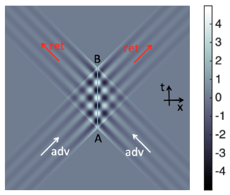
Figure 7: 2D map of $\textrm{Re}[u(x)]$ for a time symmetric monopole created at $A$ and destroyed at $B$. Advanced waves (white arrows) coming from the remote past converge to the particle at rest (vertical blue line). Retarded waves are emitted in to the future direction (red arrows). The diamond shape results from the interference between both waves and is associated with the stationary particle soliton.

An other remarkable feature of our soliton model is that it circumvents the conclusions obtained in Submitted with Ehrenfest’s theorem for a strongly localized soliton. Here our soliton associated with a monopole $\sim 1/r$ at large distance is not sufficiently localized to impose a classical-like dynamics. The deformation of the soliton obtained in our model allows him to follow a de Broglie-Bohm dynamics. Again, this is strongly related to the other features of the model discussed above. One interesting aspect of this weak localization must be emphasized. Indeed, consider a soliton at rest in free space with the monopolar field given by Eq. 31 reducing to de Broglie solution Eq. 32 in the far-field. The full energy of the soliton is given by $E=\int d^{3}\mathbf{x}[U(f^{2})-f^{2}N(f^{2})+2\omega_{0}^{2}f^{2}+\boldsymbol{\nabla}(f\boldsymbol{\nabla}f)]$ that can approximately written as

$$E\simeq E_{s}+\frac{g^{2}}{4\pi}[\omega_{0}^{2}R-\frac{\textrm{cos}^{2}(\omega_{0}R)}{R}]$$ (61)

where $E_{s}=\int d^{3}\mathbf{x}[U(f^{2})-f^{2}N(f^{2})]$ has been evaluated using the near-field, i.e., $E_{s}=\frac{g^{2}}{32r_{0}}$ (see Appendix A). The integration in Eq. 61 has been pushed until a large radius $R$. In the limit $R\rightarrow+\infty$ $E$ contains a diverging contribution growing linearly with $R$ the other term goes to zero as $1/R$. A diverging energy seems at first pathological. However, note that if the particle has a finite life-time $T$ the radius $R$ cannot grow indefinitely. As illustrated in Fig. 7 if the particle appears at $A$ (time $t=0$) and disappears at $B$ (time $t=T$) the $u$-field must have a diamond like shaped structure where advanced waves coming from the past direction interfere with retarded waves emitted to the future direction and create the stationary field of Eq. 32. The diamond structure of Fig. 7 is built between the light cones coming from past and future. Integrating the total energy at times $t<0$ or $t>T$ gives the approximate value $E\simeq\frac{g^{2}}{4\pi}\omega_{0}^{2}\frac{T}{2}$ associated with advanced or retarded waves. During the time interval $0\leq t\leq T$ we obtain $E=E_{s}+\frac{g^{2}}{4\pi}\omega_{0}^{2}\frac{T}{2}$ the difference is attributed to the local formation of the particle at $A$ requiring an additional energy $E_{s}$ coming from the environment at $A$. This energy is returning to the environment at $B$ when the particle disappears.
We can naturally speculate on the scale $R$ at which the far-field energy $E_{ff}=\frac{g^{2}}{4\pi}\omega_{0}^{2}R$ in Eq. 61 becomes comparable to $E_{s}$. The ratio $\frac{E_{ff}}{Es}=32\pi\frac{r_{0}}{\lambda_{0}}\frac{R}{\lambda_{0}}$ depends on the size of the particle $r_{0}$ and the Compton wavelength $\lambda_{0}=2\pi/\omega_{0}$. In absence of a more precise theory fixing the value of $r_{0}$ the ratio is let undetermined. Moreover, since $r_{0}$ is supposed to be very small an effect should only be observed at astrophysical or cosmological scales. For instance consider a proton with $\lambda_{0}\sim 10^{-15}$ m and suppose $R_{G}=10^{16}$ m a typical size for a galaxy. If $r_{0}$ is of the order of $r_{0}\sim 10^{-48}$ m (i.e., much smaller than the Planck length $r_{P}=10^{-35}$ m) we obtain $\frac{E_{ff}}{Es}\sim 1$. Interestingly, $R_{G}$ is the scale at which dark-matter is usually involved in order to explain the rotation curve anomaly of stars in spiral galaxy. As it is known, the density of dark-matter needed to explain the constant value of the star velocity $v_{\infty}$ at large distance of the galaxy core is typically growing as $\rho_{DM}(R)\propto 1/R^{2}$ and the mass as $M_{DM}(R)\propto R$ for $R\sim R_{G}$. This is typically what we obtain in our soliton model of quantum particles where the particle-core with energy $E_{s}$ is surrounded by a halo of energy (mass) growing as $E_{ff}\propto R$. With a value of $r_{0}\sim 10^{-48}$ m our model could thus potentially explains the anomaly in the rotation curves and interpret dark-matter as the far-field gravitational contribution of the particle masses to the dynamic of galaxies. Of course this is very speculative, and in the end it is not yet very clear what is the status of the particle energy $E$ in our theory. We point out that the conserved norm $\mathcal{Q}=\int d^{3}\mathbf{x}2\omega_{0}^{2}f^{2}$ associated with the current conservation Eq. 3b can be computed for the same example leading to Eq. 61. We get

$$\mathcal{Q}(R)\simeq\frac{g^{2}}{4\pi}[\omega_{0}R+\frac{\textrm{sin}(2\omega_{0}R)}{2}].$$ (62)

In the limit $R\rightarrow+\infty$ we obtain $\frac{E}{\mathcal{Q}}\simeq\omega_{0}[1+\frac{\lambda_{0}^{2}}{32\pi r_{0}R}]\rightarrow\omega_{0}$, i.e., $\hbar\omega_{0}$ the quantum energy formula. So perhaps it is the ratio $\frac{E}{\mathcal{Q}}$ that should be identified with the physical energy of the soliton. This could be important when considering coupling with the gravitational field where a definition of mass must be included.
To conclude this work, it is important to mention that several important questions are left open and unanswered. For example, in our model we ignored the self-electromagnetic field generated by the soliton. This can be a good approximation near the particle core but from Eq. 62 we see that the electric charge $q(R)$ contained in a sphere of radius $R$ centered on the soliton is given by $q(R)=e\mathcal{Q}(R)\simeq\frac{eg^{2}}{4\pi}\omega_{0}R$ which diverges linearly. From Gauss’s theorem this implies a radial electric field $\mathbf{E}(R)=\frac{eg^{2}}{(4\pi)^{2}}\frac{\omega_{0}}{R}\mathbf{\hat{R}}$ different from the standard Coulomb’s field. This problem could be perhaps solved by renormalizing the electric charge or by imposing the constraint $|q(R_{U})|\ll|e|$ for a large radius $R_{U}\sim 10^{26}$ m (size of the observable Universe). This implies $\frac{g^{2}}{2}\frac{R_{U}}{\lambda_{0}}\ll 1$ and for a proton we need $g^{2}\ll 10^{-41}$. If this is true we could neglect the electromagnetic coupling between solitons. New ideas should be thus inserted in the model to develop electromagnetic interactions between solitons perhaps mediated with localized solitons associated with photons. We also mention that the NLKG equation used here has some pathological features associated with the tachyonic sector alluded to briefly in Sec. 2. We restricted the analysis made in this work to the case of solitons with $\mathcal{M}_{\Psi}(z)^{2}>0$ but the tachyonic sector $\mathcal{M}_{\Psi}(z)^{2}<0$ was rejected as unphysical. Perhaps this could be avoided if the model is modified to incorporate the idea of ‘fusion’ developed by de Broglie where a spin zero particle is understood as a composite object made of two solitons with spins $1/2$. In the very end,similar approaches can certainly be developed for particles with integer spins like photons or gravitons, or with Dirac spinors for generating solitonic fermions with spin $1/2$ (this will be discussed in subsequent articles).

Appendix A

Using Eqs. 17 and 18 we define the integral

$$G=-\int d^{3}\textbf{x}N(f^{2})f=\frac{3g}{2}\int_{0}^{+\infty}d\eta\frac{\sqrt{\eta}}{(\eta+1)^{\frac{5}{2}}}$$ (63)

where $\eta=r^{2}/r_{0}^{2}$. By definition this is related to the beta Euler function $B(\frac{3}{2},1)$ by $G=\frac{3g}{2}B(\frac{3}{2},1)=\frac{3g}{2}\frac{\Gamma(\frac{3}{2})\Gamma(1)}{\Gamma(\frac{5}{2})}$ where $\Gamma(z)$ is Euler’s Gamma function. We have finally

$$G=\frac{3g}{2}\frac{\frac{\sqrt{\pi}}{2}}{\frac{3}{2}\frac{\sqrt{\pi}}{2}}=g.$$ (64)

The static energy $E_{s}$ associated with the soliton given by Eq. 18 is by definition $E_{s}=\int d^{3}\textbf{x}[(\boldsymbol{\nabla}f)^{2}+U(f^{2})]$. Inserting Eq. 17 leads after integration by part to

$$E_{s}=\int d^{3}\textbf{x}[U(f^{2})-N(f^{2})f^{2}].$$ (65)

Using Eq. 17 and Eq.16 we get

$$E_{s}=\frac{g^{2}}{4\pi r_{0}}\int_{0}^{+\infty}d\eta\frac{\sqrt{\eta}}{(\eta+1)^{3}}=\frac{g^{2}}{4\pi a}B(\frac{3}{2},\frac{3}{2})$$ (66)

which finally yields

$$E_{s}=\frac{g^{2}}{4\pi r_{0}}\frac{\Gamma(\frac{3}{2})\Gamma(\frac{3}{2})}{\Gamma(3)}=\frac{g^{2}}{4\pi r_{0}}\frac{(\frac{\sqrt{\pi}}{2})^{2}}{2}=\frac{g^{2}}{32r_{0}}.$$ (67)

Appendix B

For a static soliton $f(\mathbf{x})\in\mathbb{R}$ solution of the equation

$$\boldsymbol{\nabla}^{2}f=N(f^{2})f$$ (68)

in the 3D space we can define the static energy $E_{s}=\int d^{3}\textbf{x}[(\boldsymbol{\nabla}f)^{2}+U(f^{2})]$. $E_{s}$ can be used to establish a variational principle $\delta E_{s}=0$ for recovering the field equation $\boldsymbol{\nabla}^{2}f=N(f^{2})f$. In Hobart ; Derrick the authors consider the stretching or dilation transformation $f(\mathbf{x})\rightarrow f(\alpha\mathbf{x})$ with $\alpha$ a positive real number. Here we instead consider the more general transformation

$$f(\mathbf{x})\rightarrow\tilde{f}(\mathbf{x})=\beta f(\alpha\mathbf{x})$$ (69)

with $\beta\in\mathbb{R}$.
Under this transformation we check that the new function $\tilde{f}(\mathbf{x})$ obeys Eq. 68 iff we have $\alpha^{2}N(\tilde{f}^{2}/\beta^{2})=N(\tilde{f}^{2})$. Here we consider specifically the general Lane-Emden nonlinearity $N_{p}(x)=-\gamma x^{p}$ with $\gamma,p\in\mathbb{R}$ (the case $\gamma>0$, $p=2$ is the one considered in this article). Within this family of nonlinearity functions we obtain the constraint

$$\beta=\alpha^{1/p}$$ (70)

which reduces to $\beta=\sqrt{\alpha}$ used in the main text for $p=2$. Moreover, by using Eq. 69 and $N_{p}$ the static energy $E_{s}$ for $\tilde{f}$ becomes a function of $\alpha$ reading

$$E_{s}(\alpha)=\frac{\beta^{2}}{\alpha}I_{k}-\frac{\beta^{2(p+1)}}{\alpha^{3}}I_{p}$$ (71a)

$$=\alpha^{2/p-1}(I_{k}-I_{p})$$ (71b)

with $I_{p}=\frac{\gamma}{p+1}\int d^{3}\textbf{x}(f(\textbf{x}))^{2(p+1)}$ and $I_{k}=\int d^{3}\textbf{x}(\boldsymbol{\nabla}f(\textbf{x}))^{2}$. Importantly, in passing from Eq. 71a to 71b we used the constraint Eq. 70.
We now consider a first order variation $\delta E_{s}=E_{s}(\alpha)-E_{s}(1)$ with $\alpha=1+\epsilon$ and $\epsilon\rightarrow 0$. In Hobart ; Derrick the authors imposed $\beta=1$ and if we use Eq. 71a the variational condition $\delta E_{s}=0$ implies

$$\left.\frac{dE_{s}}{d\alpha}\right|_{\alpha=1}=-I_{k}+3I_{p}=0.$$ (72)

Therefore, we deduce $3I_{p}=I_{k}$ which is non negative by definition of $I_{k}$ and implies $\gamma>0$. Similarly, we can define a second order variation $\delta^{2}E_{s}$ and we obtain

$$\left.\frac{d^{2}E_{s}}{d\alpha^{2}}\right|_{\alpha=1}=2I_{k}-12I_{p}=-6I_{p}<0.$$ (73)

This implies unstability of the soliton. However, a physical transformation for this soliton must rely on the constraint Eq. 70 in order to fulfill Eq. 71b. Therefore instead of Eq. 72 we must have:

$$\left.\frac{dE_{s}}{d\alpha}\right|_{\alpha=1}=(2/p-1)(I_{k}-I_{p})=0.$$ (74)

Moreover, we have $I_{k}-I_{p}=E_{s}(1)$ and $I_{k}=(p+1)I_{p}$ (as it can be checked after integration by parts of $I_{k}$ and neglecting a surface integral term) and we thus get $(2/p-1)pI_{p}=0$ which imposes the value $p=2$ (this result was obtained in Rosen1966 ). Observe that if we insert the formula $I_{k}=(p+1)I_{p}$ in Eq. 72 we obtain $-(p+1)I_{p}+3I_{p}=0$ and therefore we again deduce the condition $p=2$ which is thus imposed by either Eq. 72 or Eq. 74. This result assumes that the field decays fast enough (i.e., at least as $f\sim 1/r^{m}$ with $m>1/2$ for $r$ large) in order to neglect the surface integral term in $I_{k}$. Furthermore, with Eq. 71b we obtain

$$\left.\frac{d^{2}E_{s}}{d\alpha^{2}}\right|_{\alpha=1}=(2/p-1)(2/p-2)(I_{k}-I_{p}).$$ (75)

replacing Eq. 73. Clearly, from Eq. 74 we deduce $\left.\frac{d^{2}E_{s}}{d\alpha^{2}}\right|_{\alpha=1}=0$ which means that the soliton is not anymore unstable: it is metastable. This result evades the conclusions of the Hobart-Derrick theorem which was established without using the legitimate dilation transformation Eq. 70.

Appendix C

We start with the local current conservation $\partial_{\mu}(f^{2}(x)\mathcal{M}_{u}(x)v_{u}^{\mu}(x))=0$. Consider now the 4D volume sketched in Fig. 8 which is bound by i) the two hyperplanes $\Sigma(\tau)$ and $\Sigma(\tau+\delta\tau)$ normal to respectively $\dot{z}(\tau)$ and $\dot{z}(\tau+\delta\tau)$ (with $\delta\tau$ an infinitesimal delay time), and ii) the cylindrical hypersurface $S$ surrounding the particle trajectory. This hypersurface $S$ is a 3D object which projects as a 2D closed surface surrounding the particle position $\mathbf{z}(\tau)$ in the hyperplane $\Sigma(\tau)$.

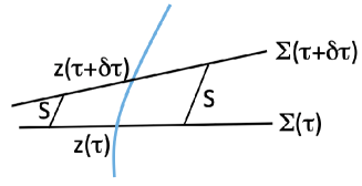
Figure 8: Sketch of the 4D volume surrounding the particle trajectory $z(\tau)$ as discussed in the main text.

The local height $\delta t$ of the cylinder is given by Submitted $\delta t=\delta\tau(1-\xi\ddot{z}(\tau))$. A direct application of Gauss’s theorem applied to $\partial_{\mu}(f^{2}(x)\mathcal{M}_{u}(x)v_{u}^{\mu}(x))=0$ in this 4D volume in space-time leads to

$$\int_{\Sigma(\tau+\delta\tau)}f^{2}(x)\mathcal{M}_{u}(x)v^{\mu}_{u}(x)\cdot\dot{z}_{\mu}(\tau+\delta\tau)d^{3}\sigma$$

$$-\int_{\Sigma(\tau)}f^{2}(x)\mathcal{M}_{u}(x)v^{\mu}_{u}(x)\cdot\dot{z}_{\mu}(\tau)d^{3}\sigma$$

$$=\oint_{S}d^{2}S_{\mu}v_{u}^{\mu}(x)(1-\xi\ddot{z}(\tau))\delta\tau\mathcal{M}_{u}(x)$$ (76)

with $d^{2}S^{\mu}:=[0,d^{2}\mathbf{S}]$ a 4-vector associated with the local surface $d^{2}\mathbf{S}$ of the 2D surface surrounding $\mathbf{z}(\tau)$. We have

$$\oint_{S}d^{2}S_{\mu}v_{u}^{\mu}(x)(1-\xi\ddot{z}(\tau))\delta\tau\mathcal{M}_{u}(x)$$

$$=-\oint_{S}d^{2}\mathbf{S}\cdot\mathbf{v}_{u}(x)[1+\boldsymbol{\xi}\cdot\ddot{\mathbf{z}}]\delta\tau\mathcal{M}_{u}(x).$$ (77)

Moreover, we have near the soliton center $\mathbf{v}_{(}x)\simeq O(\boldsymbol{\xi})$. Therefore, writing $d^{2}\mathbf{S}=\boldsymbol{\xi}^{2}d^{2}\Omega$ (where $d^{2}\Omega$ is an elementary solid angle) the surface integral in Eq. 77 is varying like $O(\xi^{3})$ which is neglected. Similarly, for the scalar products of the velocities we have $v^{\mu}_{u}(x)\cdot\dot{z}_{\mu}(\tau+\delta\tau)\simeq 1$ and $v^{\mu}_{u}(x)\cdot\dot{z}_{\mu}(\tau)\simeq 1$ and Eq. 77 reduces to:

$$\frac{d}{d\tau}\int_{\Sigma(\tau)}f^{2}(x)\mathcal{M}_{u}(x)d^{3}\sigma\simeq 0$$ (78)

which leads to

$$\int_{\Sigma(\tau)}f^{2}(x)\mathcal{M}_{u}(x)d^{3}\sigma=C$$ (79)

where $C$ is a constant (assuming the volume small).
Now, writing $\mathcal{M}_{u}(x)\simeq\mathcal{M}_{\Psi}(z(\tau))$ and using Eq. 23 we have $f(x)=F_{\tau}(r)=\sqrt{\alpha(\tau)}F_{0}(\alpha(\tau)r)$. After using the variable $\mathbf{w}=\alpha(\tau)\boldsymbol{\xi}$ we have

$$C=\mathcal{M}_{\Psi}(z(\tau))\frac{1}{\alpha^{2}(\tau)}\int F_{0}(w)d^{3}\boldsymbol{w}$$ (80)

which directly leads to Eq. 25.

Appendix D

Local energy-momentum conservation for the field of Eq. 1 can be written in different equivalent ways. Here using the hydrodynamic formalism we introduce a energy-momentum tensor $T^{\mu\nu}(x)=2f^{2}(x)\mathcal{M}_{u}^{2}(x)v_{u}^{\mu}(x)v_{u}^{\nu}(x)$ obeying the conservation law:

$$\partial_{\mu}T^{\mu\nu}=2f^{2}\mathcal{M}_{u}\frac{d}{d\tau_{u}}(\mathcal{M}_{u}v_{u}^{\nu})=2f^{2}\mathcal{M}_{u}[\partial^{\nu}(\mathcal{M}_{u})+eF^{\nu\mu}{v_{u}}_{\mu}]$$ (81)

with $\frac{d}{d\tau_{u}}:=v_{u}^{\mu}\partial_{\mu}$. We used the current conservation to obtain the first equality. This leads to $\frac{d}{d\tau_{u}}(\mathcal{M}_{u}v_{u}^{\nu})=\partial^{\nu}(\mathcal{M}_{u})+eF^{\nu\mu}{v_{u}}_{\mu}$ that can be obtained directly from Eq. 3a and represents a quantum generalization of Newton’s force formula for the $u-$field.
A different way to write the energy-momentum conservation law is:

$$\partial_{\mu}[T_{0}^{\mu\nu}+\eta^{\mu\nu}V(f^{2})]=2ef^{2}\mathcal{M}_{u}F^{\nu\mu}{v_{u}}_{\mu}$$ (82)

with $T_{0}^{\mu\nu}=T^{\mu\nu}+2\partial^{\mu}f\partial^{\nu}f-\eta^{\mu\nu}[(\partial f)^{2}+f^{2}\mathcal{M}_{u}^{2}]$. Finally, if we consider the full Maxwell’s equations we have $\partial_{\mu}F^{\mu\nu}=2ef^{2}\mathcal{M}_{u}{v_{u}}^{\nu}$ and therefore if we write $T_{em}^{\mu\nu}$ the standard electromagnetic field energy-momentum tensor we must have $\partial_{\mu}T_{em}^{\mu\nu}=-2ef^{2}\mathcal{M}_{u}F^{\nu\mu}{v_{u}}_{\mu}$. In the end we get:

$$\partial_{\mu}[T_{0}^{\mu\nu}+\eta^{\mu\nu}V(f^{2})+T_{em}^{\mu\nu}]=0.$$ (83)

In the Appendix D of Submitted we applied Gauss’s theorem to Eq. 81 in a 4-D world tube surrounding the trajectory $z(\tau)$ of a soliton with two ending (3D) spacelike hyper-surfaces $\delta\Sigma_{A}$ and $\delta\Sigma_{B}$, and obtained:

$$\int_{\delta\Sigma_{B}}2f^{2}(x)\mathcal{M}_{u}^{2}v_{u}^{\nu}-\int_{\delta\Sigma_{A}}2f^{2}(x)\mathcal{M}_{u}^{2}v_{u}^{\nu}$$ (84)

$$=\int_{A}^{B}d\tau\int_{\Sigma_{0}(\tau)}d^{3}\sigma_{0}2f^{2}\mathcal{M}_{u}[\partial^{\nu}\mathcal{M}_{u}+eF^{\nu\mu}{v_{\nu}}_{u}].$$ (85)

In Submitted we showed that for a strongly localized soliton like an undeformable Gausson this relation leads to a form of Ehrenfest’s theorem where the quantum potential term cancels out because the $u-$field amplitude decays exponentially far away from $z(\tau)$. In the present work with a weakly localized soliton with $f\sim 1/r$ at large distance from $z(\tau)$ we can not apply this result. Moreover, taking infinitely small cross-sections $\delta\Sigma_{\tau}$ for the tube and using the fact that near the trajectory $z(\tau)$ we have (see the footnote 2): $\mathcal{M}_{u}(x)\simeq\mathcal{M}_{\Psi}(z(\tau))+\boldsymbol{\xi}\cdot\boldsymbol{\nabla}\mathcal{M}_{\Psi}(z(\tau))+O(\xi^{2})$, $\partial_{\mu}\mathcal{M}_{u}(z(\tau))=\partial_{\mu}\mathcal{M}_{\Psi}(z(\tau))$. This can be easily used to justify once more the dynamical law $\frac{d}{d\tau_{u}}(\mathcal{M}_{\psi}(z)\dot{z}^{\nu})=\partial^{\nu}(\mathcal{M}_{\psi}(z))+eF^{\nu\mu}\dot{z}_{\mu}$ associated with the PWI.

Competing Interest

The Author declares no competing interest for this work.

Data Availability Statement

Data Availability Statement: No Data associated in the manuscript.

References

- (1) G. Bacciagaluppi, A. Valentini,Quantum theory at the crossroads: Reconsidering the 1927 Solvay Conference (Cambridge Univ. Press, Cambridge, 2009).
- (2) O. Costa de Beauregard, C. R. Acad. Sci 236, 1632 (1953).
- (3) I. Bialynicki-Birula and J. Mycielski, Ann. Phys. 100, 62-93 (1976).
- (4) D. Bohm, Phys. Rev. 85, 166–179 (1952).
- (5) D. Bohm and B. J. Hiley, The undivided Universe (Routledge, London, 1993).
- (6) L. de Broglie, C. R. Acad. Sci. (Paris) 180, 498-500 (1925).
- (7) L. de Broglie, Ondes et mouvements (Gauthier-Villars, Paris, 1926).
- (8) L. de Broglie, J. Phys. Radium 8, 225-241 (1927); translated in: L. de Broglie, and L. Brillouin, Selected papers on wave mechanics (Blackie and Son, Glasgow, 1928).
- (9) L. de Broglie, Une tentative d’interprétation causale et non linéaire de la mécanique ondulatoire: la théorie de la double solution (Gauthier-Villars, Paris 1956); translated in: L. de Broglie, Nonlinear wave mechanics: A causal interpretation (Elsevier, Amsterdam, 1960).
- (10) S. Chandrasekhar, An introduction to the study of stellar structures, chap. 4 (University of Chicago Press, Chicago, 1939).
- (11) S. Collin, T. Durt, R. Willox, Ann. Fond. de Broglie 42, 19-70 (2017).
- (12) G. H. Derrick, J. Math. Phys. 5, 1252-1254 (1964).
- (13) P. A. M. Dirac, Proc. R. Soc. Lond. A 167, 148-169 (1938).
- (14) A. Drezet, Found. Phys. 49,1166-1199 (2019).
- (15) A. Drezet, Ann. Fond. de Broglie 46, 65-85 (2021).
- (16) A. Drezet, Quantum solitodynamics: Non-linear wave mechanics and pilot-wave theory, arXiv:2205.04706
- (17) D. Fargue, in The wave-particle dualism (S. Diner et al. Eds.), p. 149-172, D. Reidel Publishing, 1984.
- (18) D. Fargue, Ann. Fond. de Broglie 42, 9-18 (2017).
- (19) F. Fer, Doctorate Thesis, Bureau de documentation minière, Paris (1957).
- (20) F. Fer, in L. de Broglie, sa conception du monde physique p. 279, Paris (1973).
- (21) A.D. Fokker, Z. Phys. 58, 386-393 (1929).
- (22) J. Goldstone, R. Jackiw, Phys. Rev. D 11, 1486-1498 (1975).
- (23) R. H. Hobart, Proc. Phys. Soc. 82, 201-203 (1963).
- (24) F. Hoyle, J.V. Narlikar, Rev. Mod . Phys. 67, 113-155 (1995).
- (25) G. Mie, Ann. der Phys. (Berlin) 99, 1-40 (1912).
- (26) L. Page, Phys. Rev. 18, 292 (1921).
- (27) G. Petiau, C. R. Acad. Sci. (Paris) 239, 344-346 (1954).
- (28) G. Petiau, Séminaire L. de Broglie: Théories Physiques (Paris) 24, exposé 18 (1954-1955).
- (29) G. Petiau, C. R. Acad. Sci. (Paris) 239, 2491-2493 (1955).
- (30) G. Rosen, J. Math. Phys. 6, 1269-1272 (1965).
- (31) G. Rosen, J. Math. Phys. 7, 2066-2070 (1966).
- (32) Yu. P. Rybakov, R. Saha, Found. Phys. 25, 1723-1731 (1995).
- (33) J. Schwinger, Found. Phys. 13, 373-383 (1983).
- (34) H. Tetrode, Z. Phys. 10, 317-328 (1922).
- (35) J.A. Wheeler, and R.P. Feynman, Rev. Mod. Phys 17, 157-181 (1945).