Towards coarse-grained elasticity of single-layer Covalent Organic Frameworks

Abstract

Two-dimensional covalent organic frameworks (2D COFs) are an interesting class of 2D materials since their reticular synthesis allows the tailored design of structures and functionalities. For many of their applications the mechanical stability and performance is an important aspect. Here, we use a computational approach involving a density-functional based tight-binding method to calculate the in-plane elastic properties of about 40 COFs with a honeycomb lattice. Based on those calculations, we develop two coarse-grained descriptions: one based on a spring network and the second using a network of elastic beams. The models allow us to connect the COF force constants to the molecular force constants of the linker molecules and thus enable an efficient description of elastic deformations. To illustrate this aspect, we calculate the deformation energy of different COFs containing the equivalent of a Stone-Wales defect and find very good agreement with the coarse-grained description.

1 Introduction

Two-dimensional covalent organic frameworks (2D COFs) are nanostructured porous crystals and have shown considerable potential for applications in many fields [1, 2, 3, 4, 5, 6]. They consist of networks formed by covalently linked organic molecules made from light elements such as carbon, nitrogen, boron and oxygen. This specific molecular architecture gives them a high mechanical, thermal and chemical stability [7]. The underlying reticular chemistry allows it to combine different building blocks to obtain specific topologies and properties [3, 4, 5, 6]. Compared to their inorganic cousins, e.g. TMDCs, this leads to a much larger variety of possible materials but also requires more sophisticated synthesis strategies [8, 9, 10, 11, 12, 13, 14, 15, 16, 17, 18].

Although many properties of 2D COFs, and in particular structural and elastic properties [19, 20, 21], can be calculated using a range of different methods, the large number of atoms in the unit-cell and the combinatorial wealth of possible COFs still poses a challenge. Moreover, for COFs containing defects, like single 5+7 defects [22] or extended grain boundaries [23, 24], a full atomistic description quickly becomes unfeasible and coarse-grained treatments are unavoidable. Recently, we have proposed one such approach in the context of elasticity where the COFs are treated as an effective spring network and the spring constants are obtained directly from the individual building blocks [25]. For several COFs with square-lattice geometry, we could predict the 2D bulk-modulus from the molecular spring constants.

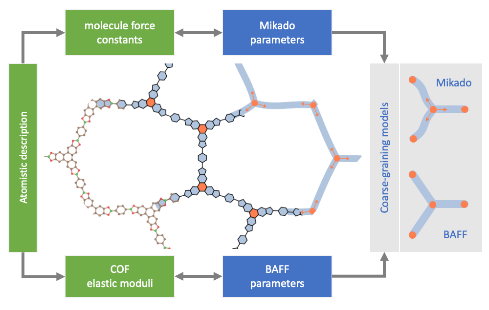
Figure 1: Schematic view of the coarse-graining approach: From the atomistic description of the COF the elastic moduli are computed and used to obtain the parameters of the bond and angle force field (BAFF) which uses only the positions of the cores (orange areas) to get lengths of the linkers (blue areas) and angles between them. Additionally, the force constants of linker molecules are used to determine the parameters of the Mikado model. Here, the linker molecules are represented by elastic beams which are cross-linked at the cores. The latter are considered as rigid molecules having a position and an orientation (arrows). In the center a Tp DB-COF (or COF-5) with a Stone-Wales defect is shown as an example. Carbon atoms are colored brown, oxygen red and boron green. Hydrogen atoms are not shown for convenience.

In this article we focus on COFs with honeycomb lattices since their material properties are expected to be isotropic [26]. In addition to the bulk modulus we also consider the shear modulus and thus achieve a complete characterization of the in-plane elasticity of those materials. Using a description in terms of a coarse-grained spring network which includes bond-stretching and angle-bending contributions, we can connect the effective force constants of the network to the elastic moduli (see Fig. 1). In order to better account for the flexibility of the linker molecules, we develop a second model which is based on treating them as 2D elastic beams. This model, which is inspired by the well-known Mikado model [27, 28] and beam-network models [29, 30], allows it to understand the relation of bulk and shear moduli with lattice constant of the COFs and provides a connection of the COF elasticity with the molecular properties. Both coarse-grained descriptions can also be applied to structures with defects. To validate and benchmark the models we performed calculations with the density functional-based tight-binding method (DFTB) [31, 32] for about forty COFs and their building-blocks. In three cases we introduce the equivalent of a Stone-Wales defect [33] into the crystal and compute the resulting deformation energies.

][c]0.53

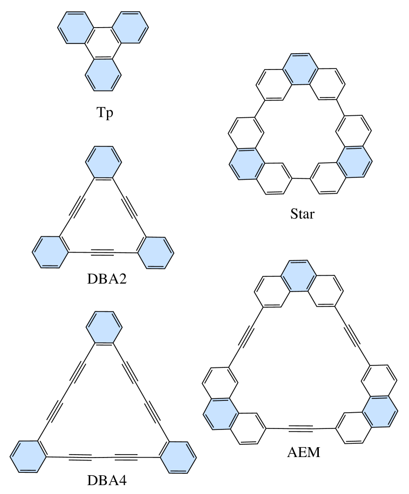
(a)

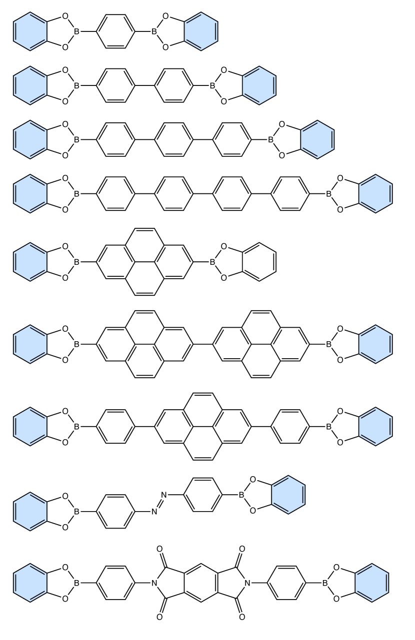
(b)

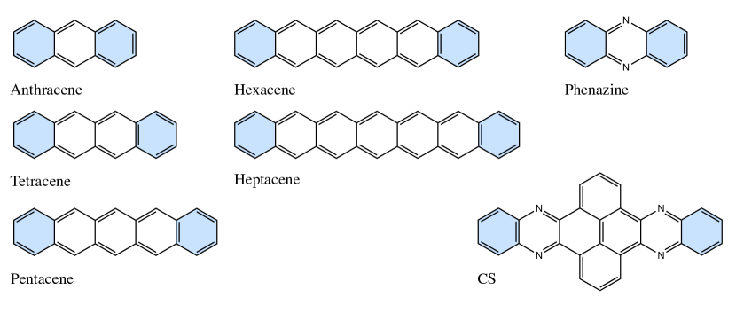
(c)

Figure 2: Cores and linker molecules. The blue colored phenyl rings are shared between core and linkers. (a) Five cores with $C_{3}$ symmetry are used in this work: Triphenylene (Tp), Star, AEM, DBA2, and DBA4. (b) Linker molecules containing boronate ester, from top to bottom: DB 1phenyl, DB 2phenyls, DB 3phenyls, DB 4phenyls, DB 1pyrene, DB 2pyrenes, DB phenyl pyrene phenyl, DB Azobenzene, and DB ANDI. (c) Linker molecules only used with Tp core: Anthracene, Tetracene, Pentacene, Hexacene, Heptacene, Phenazine, and pyrene-fused tetraazahexacene (CS).

The specific COFs studied in this work include five molecular cores with $C_{3}$ symmetry and different linear linker molecules. In Fig. 2 the molecular building-blocks are shown together with the respective linker molecule used for the computational model. It should be noted that those linkers are not necessarily identical to the building-blocks used for the polymerization. Instead, our nomenclature reflects the structure of the resulting COFs. We consistently denote them as core–linker–COF, for example, COF-10 is denoted as Tp–DB 2phenyls–COF. The COFs under consideration include Tp–DB 1phenyl–COF (known as COF-5) [34], Star-COF [35], DBA2- and DBA4-COF [36], and AEM-COF [37]. In order to obtain linkers with a larger variability of lengths, we keep the molecular structure but change the number of phenyls or pyrenes in the linkers [38, 39], as shown in Fig. 2(b). Additionally, we consider linkers based on fused acenes, phenazine and pyrene-fused tetraazahexacene [40, 41, 42].

The article is structured as follows. In section 2, the two coarse-grained models are introduced and expressions for the elastic moduli and force constants are derived. In the next section, the computational details are provided. Section 4 contains the presentation and discussion of the results. Conclusions are provided in the last section.

2 Elasticity of honeycomb 2D COFs

2.1 Elastic moduli of coarse-grained spring networks

A straight-forward coarse-graining description of a COF consists in treating the cores as sites of a lattice. Those sites have only translational degrees of freedom and are mutually connected via the linkers, which are not further characterized. More specifically, we consider a honeycomb lattice with interactions between neighboring sites $i$ and $j$ (stretching contribution) and between neighboring bonds (angle bending contribution). The elastic energy of the resulting Bond and Angle Force Field (BAFF) reads [43]

$$\mathcal{H}_{\rm total} ={} \sum_{i,j}\frac{\beta_{r}}{\ell_{0}^{2}}(\ell_{ij}-\ell_{0})^{2}+\sum_{i,j<k}\beta_{c}(\cos(\phi_{jik})-\cos(\phi_{0}))^{2}$$ (1)

$$={} \frac{1}{2}\sum_{b}\frac{4\beta_{r}}{\ell_{0}^{2}}(\ell_{b}-\ell_{0})^{2}+\sum_{b,b^{\prime}}\frac{3\beta_{c}}{8}(\phi_{bb^{\prime}}-\phi_{0})^{2}\;,$$

where $\ell_{ij}=|\vec{R}_{i}-\vec{R}_{j}|$ is the distance between sites $i$ and $j$, $\phi_{jik}$ is the angle between the bond-vectors $\vec{R}_{ij}=\vec{R}_{j}-\vec{R}_{i}$ and $\vec{R}_{ik}=\vec{R}_{k}-\vec{R}_{i}$, and $\ell_{0}$ and $\phi_{0}$ are the equilibrium values. In the second line, summations are over bonds, $b$ and $b^{\prime}$, instead of sites and the bending term was expanded for angles close to the equilibrium.

In terms of the force constants $\beta_{r}$ and $\beta_{c}$ the 2D bulk and shear modulus are [43]

$$B_{2D}={} \frac{4\beta_{r}}{2\sqrt{3}\ell_{0}^{2}}=\frac{k}{2\sqrt{3}}\;,$$ (2a)

$$\mu_{2D}={} {3}\sqrt{3}\frac{k\beta_{c}/\ell_{0}^{2}}{k+9\beta_{c}/\ell_{0}^{2}}=\frac{1}{\sqrt{3}}\frac{k\kappa}{k+\kappa}=\frac{1}{\sqrt{3}}\left(\frac{1}{k}+\frac{1}{\kappa}\right)^{-1}\;.$$ (2b)

The bulk modulus $B_{2D}$ only depends on the stretching force-constant $k=4\beta_{r}/\ell_{0}^{2}$, while the shear modulus $\mu_{2D}$ is determined by $k$ and the effective angle-bending constant $\kappa=9\beta_{c}/\ell_{0}^{2}$.

Due to the honeycomb symmetry, all in-plane elastic constants can be expressed in terms of $B_{2D}$ and $\mu_{2D}$ [26]. In particular, the non-vanishing elements of the stiffness tensor are (see also supporting information)

$$C_{11}={} C_{22}=B_{2D}+\mu_{2D}\;,$$ (2ca)

$$C_{12}={} C_{21}=B_{2D}-\mu_{2D}\;,$$ (2cb)

$$C_{66}={} (C_{11}-C_{12})/2=\mu_{2D}\;.$$ (2cc)

Finally, the Young modulus $Y_{2D}$ and the Poisson ratio $\nu_{2D}$ can be obtained via

$$Y_{2D}=\frac{4B_{2D}\mu_{2D}}{B_{2D}+\mu_{2D}}\quad{\rm and}\quad\nu_{2D}=\frac{B_{2D}-\mu_{2D}}{B_{2D}+\mu_{2D}}\;.$$ (2cd)

Note, that the energy given by Eq. (1) does not contain terms which penalize out of plane bending and therefore the bending rigidities vanish within this model.

2.2 Stretching and bending moduli of semi-flexible polymers

Two-dimensional COFs are basically cross-linked semiflexible polymer networks where the cross-links are located on a 2D surface. A very successful model of random networks is the Mikado model [27, 28, 44], where it is assumed that the network is formed by fibers which are cross-linked at the intersection of two such fibers (cf. Fig. 1). The individual fibers are modeled as elastic beams and their energy under deformation is given by:

$$\mathcal{H}_{\rm fiber}=\int_{0}^{\ell_{0}}ds\left\{\frac{c_{\rm stretch}}{2}\left(\frac{\partial u_{\|}(s)}{\partial s}\right)^{2}+\frac{c_{\rm bend}}{2}\left(\frac{\partial^{2}u_{\perp}(s)}{\partial s^{2}}\right)^{2}\right\}\;,$$ (2ce)

where $s$ denotes the position along the fiber axis and $u_{\|}$ and $u_{\perp}$ are the tangential and transverse displacements with respect to the fiber axis. The first contribution describes the stretching energy, which results from changing the length of the fiber, while the second term is the bending energy. The two corresponding elastic moduli are $c_{\rm stretch}$ and $c_{\rm bend}$. For an elastic beam the two moduli are related, but here we treat them as independent molecule-specific constants. More details can be found in the supporting information.

For a homogeneous elongation or compression of the fiber, i.e. $u_{\|}(s)=\frac{\Delta\ell}{\ell_{0}}s$, the stretching energy becomes:

$$\mathcal{H}_{\rm stretch}=\frac{1}{2}c_{\rm stretch}\ell_{0}\left(\frac{\Delta\ell}{\ell_{0}}\right)^{2}=\frac{1}{2}\frac{c_{\rm stretch}}{{\ell_{0}}}{\Delta\ell^{2}}\;,$$ (2cf)

which corresponds to a Hookean spring with spring constant $k_{\rm fiber}=c_{\rm stretch}/\ell_{0}$. The nature of the bending deformation will depend on the cross-linking, which determines the boundary conditions for $u_{\perp}$ at the end-points: $u_{\perp}(0)$, $u_{\perp}(\ell_{0})$, $\varphi(0)$, and $\varphi(\ell_{0})$. The latter two denote the derivative of $u_{\perp}$, i.e., $\varphi(s)=\partial u_{\perp}/\partial s$. In terms of those boundary values, the transverse displacement is

$$u_{\perp}(s)={} \left(\frac{\varphi(0)+\varphi(\ell_{0})}{\ell_{0}^{2}}-2\frac{u_{\perp}(\ell_{0})-u_{\perp}(0)}{\ell_{0}^{3}}\right)s^{3}$$ (2cg)

$$+\left(-\frac{2\varphi(0)+\varphi(\ell_{0})}{\ell_{0}}+3\frac{u_{\perp}(\ell_{0})-u_{\perp}(0)}{\ell_{0}^{2}}\right)s^{2}$$

$$+\varphi(0)s+u_{\perp}(0)\;.$$

This expression leads to the in-plane bending energy of the fiber as follows:

$$\mathcal{H}_{\rm bend}={} \frac{1}{2}\frac{12c_{\rm bend}}{\ell_{0}^{3}}\left[\left(u_{\perp}(\ell_{0})-u_{\perp}(0)\right)^{2}\right.$$ (2ch)

$$+\frac{\ell_{0}^{2}}{3}\left(\varphi(0)^{2}+\varphi(0)\varphi(\ell_{0})+\varphi(\ell_{0})^{2}\right)$$

$$\left.-\ell_{0}\left(u_{\perp}(\ell_{0})-u_{\perp}(0)\right)\left(\varphi(\ell_{0})+\varphi(0)\right)\right]\;.$$

If the endpoints of the fiber are displaced relatively by $\Delta=u_{\perp}(\ell_{0})-u_{\perp}(0)$ while keeping $\varphi(0)=\varphi(\ell_{0})=0$, the effective in-plane bending force-constant becomes $\kappa_{\rm fiber}={12c_{\rm bend}}/{\ell_{0}^{3}}$, which scales as $\ell_{0}^{-3}$. If $\varphi$ at the ends is allowed to change, it is beneficial to switch to the variables $\psi(0)=\varphi(0)-\Delta/\ell_{0}$ and $\psi(\ell_{0})=\varphi(\ell_{0})-\Delta/\ell_{0}$. This leads to

$$\mathcal{H}_{\rm bend}=\frac{1}{2}\frac{4c_{\rm bend}}{\ell_{0}}\left[\psi(0)^{2}+\psi(0)\psi(\ell_{0})+\psi(\ell_{0})^{2}\right]\;,$$ (2ci)

which makes it clear that without constraints the fiber tends to a straight configuration ($\psi(0)=\psi(\ell_{0})=0$) with vanishing bending energy.

2.3 Moduli of polymer networks

In polymer networks the fibers are connected at cross-links which are typically considered as rigid joints implying that they have translational and rotational degrees of freedom, but are not deformable [29, 30]. Using the results for single fibers presented in the previous section, we can obtain the effective spring and bending constants ($k$ and $\kappa$) and thus the elastic moduli of the network. The stretching energy is simply given by the sum of individual fiber contributions (cf. Eq. (2cf)) and $k=k_{\rm fiber}$. In order to determine the deformation energy of angle bending, we consider two straight fibers (denoted A and B) of length $\ell_{0}$ which are linked at a rigid joint (at $s=0$). Displacing the endpoint of one fiber (A) perpendicular to the fiber axis by $\Delta$ changes the angle between the fibers from $\phi_{0}$ to $\phi=\phi_{0}+\Delta/\ell_{0}$. According to Eq. (1) the deformation energy is

$$\mathcal{H}_{\rm angle}=\frac{3\beta_{c}}{2}\left(\frac{\Delta}{\ell_{0}}\right)^{2}\;.$$ (2cj)

On the other hand, adding the in-plane bending energies (2ci) for both fibers yields

$$\mathcal{H}_{\rm angle}={} \frac{2c_{\rm bend}}{\ell_{0}}\left[\psi_{A}(0)^{2}+\psi_{A}(0)\psi_{A}(\ell_{0})+\psi_{A}(\ell_{0})^{2}\right.$$ (2ck)

$$\left.+\psi_{B}(0)^{2}+\psi_{B}(0)\psi_{B}(\ell_{0})+\psi_{B}(\ell_{0})^{2}\right]\;.$$

Since the fibers are linked at $s=0$, the constraint $\psi_{A}(0)=\psi_{B}(0)+\phi_{0}-\phi=\psi_{B}(0)-\Delta/\ell_{0}$ holds. If the deformation is such that fiber B remains straight ($\psi_{B}(\ell_{0})=\psi_{B}(0)=0$) and $\psi_{A}(\ell_{0})=0$, the comparison of the deformation energies (2cj) and (2ck) gives

$$\frac{3\beta_{c}}{2}=\frac{2c_{\rm bend}}{\ell_{0}}\quad\Longleftrightarrow\quad\kappa=\frac{9\beta_{c}}{\ell_{0}^{2}}=\frac{12c_{\rm bend}}{\ell_{0}^{3}}=\kappa_{\rm fiber}\;.$$ (2cl)

Based on the expressions above, the total energy of the deformed polymer network is given as a sum of the individual fiber contributions:

$$\mathcal{H}_{\rm total}=\sum_{b}\left\{\frac{1}{2}k_{\rm fiber}{\Delta\ell_{b}^{2}}+\frac{\ell_{0}^{2}\kappa_{\rm fiber}}{6}\left[\psi_{b}(0)^{2}+\psi_{b}(0)\psi_{b}(\ell_{0})+\psi_{b}(\ell_{0})^{2}\right]\right\}\;.$$ (2cm)

Additionally, at each joint the constraint

$$\psi_{b}(0)-\psi_{b^{\prime}}(0)=\phi_{0}-\phi_{bb^{\prime}}$$ (2cn)

has to hold for all $n_{j}$ neighboring fibers $b$ and $b^{\prime}$. Those $n_{j}-1$ independent conditions determine all $\psi$ at that joint in terms of its orientation. The corresponding orientation vector $\vec{\omega}$ is set to point along one of the fibers in the undeformed state (all $\phi_{bb^{\prime}}=\phi_{0}$). Then, the angle between $\vec{\omega}$ and the direction of the chosen fiber $b$ determines $\psi_{b}$ as explained in the supplementary information.

3 Computational details

In this work, we use DFTB with self-consistent charge extension (SCC) method [31, 32] to compute the elastic properties of COFs and monomers, as implemented in the DFTB+ code (version 20.2). For all calculations we use the matsci-0-3 parametrization [45]. For the COF calculations, periodic boundary conditions were used. Single layers were optimized using the SCC method with $30~{}\textrm{\AA}$ distance between the layers to avoid interactions between them. The $k$-points according to Monkhorst and Pack [46] were generated by using a $k$-spacing of $0.3~{}\textrm{\AA}^{-1}$ where the resulting k-point grid was rounded to its next integer value. A convergence criterion for the SCC cycles of $10^{-8}~{}\textrm{e}$ and a maximum force component of $10^{-5}~{}\textrm{Hartree}/\textrm{bohr}$ was chosen. To determine the bulk and the shear moduli, the primitive cell was biaxially strained starting from the equilibrium configuration in steps of $0.2$%, while the $z$-direction of the lattice vector was always remaining the same. The moduli were then determined from the total energy by fitting a cubic polynomial to the area-energy relations for the bulk or the strain-energy relations for the shear modulus [25]. The deformation energy of COFs with SW defect was obtained for $3\times 3$ supercells and using one k-point centered at the $\Gamma$-point during the geometry optimization with $10^{-5}~{}\textrm{e}$ and $10^{-5}~{}\textrm{Hartree}/\textrm{bohr}$ as convergence criteria.

Similarly, the molecular spring and bending constants were obtained from SCC DFTB calculations. We fixed the two outermost hydrogen and carbon atoms of the molecular linkers and relaxed the remaining atom positions. For obtaining the stretching force constant, we elongate and compress the molecule by moving the fixed atoms in steps of $0.2$Å along the molecular axis. The force constant is then found from the energy-displacement curve via Eq. (2cf). The bending force constant is found by moving the fixed atoms perpendicular to the molecular axis and then using Eq. (2ch).

4 Results and Discussion

4.1 Bulk and shear moduli

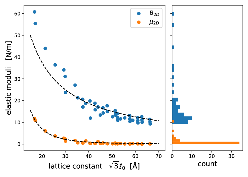
Figure 3: Lattice constant dependence of the COF elastic moduli $B_{2D}$ and $\mu_{2D}$. The dashed lines are guides to the eye (no fitting involved). The right panel shows the distribution of the elastic moduli for the COFs under consideration.

The bulk and shear moduli have been calculated for the core and linker combinations shown in Fig. 2. The respective results are summarized in Fig. 3 and are listed in table 1 for a selection of COFs (see SI for the full list). Compared to graphene, the moduli of the COFs are smaller by a factor 4 to 20, but are similar to the moduli of some inorganic 2D materials. For example, the computational 2D materials database [47] gives for hexagonal PbSe₂ the moduli $B_{2D}=23.89$ N/m and $\mu_{2D}=1.13$ N/m. As a general trend, the moduli decrease with increasing lattice constant. Apparently, this behavior follows a systematic trend which is indicated in Fig. 3 by the dashed lines.

T

COF Name	$a$ [Å]	$B_{2D}$ [N/m]	$\mu_{2D}$ [N/m]	$k$ [N/m]	$\kappa$ [N/m]
Tp–Anthracene	17.125	55.39	10.82	191.88	20.76
Tp–DB 1phenyl	30.083	23.67	1.38	82.00	2.46
DBA2–DB 1phenyl	35.339	21.27	0.59	73.66	1.03
DBA4–DB 1phenyl	40.556	19.83	0.35	68.68	0.61
Star–DB 1phenyl	38.762	18.65	1.47	64.62	2.64
AEM–DB 1phenyl	43.998	17.07	1.24	59.12	2.22

Table 1: DFTB results for different COFs: lattice constant ($a$), bulk and shear moduli ($B_{2D}$ and $\mu_{2D}$), and the effective spring and bending constants ($k$ and $\kappa$) obtained from Eqs. (2).

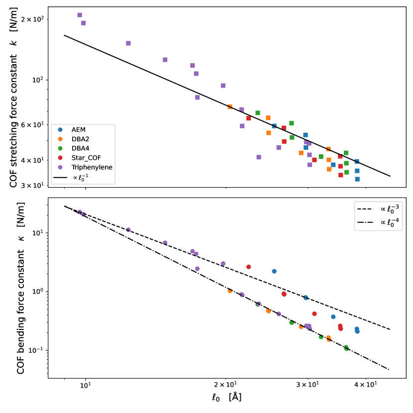
Figure 4: Length dependence of the COF force constants $k$ (top) and $\kappa$ (bottom). The length of the linker is obtained from the lattice constant $\ell_{0}=a/\sqrt{3}$.

In order to understand the described behavior, we use Eqs. (2) to obtain the effective stretching and bending force constants, $k$ and $\kappa$, for each COF. Figure 4 shows their dependence on the length of the respective linker which is calculated from the lattice constant as $\ell_{0}=a/\sqrt{3}$. One can see that both force constants decrease as the length of the linker is increased. For all COFs, the stretching force constant $k$ is found to be inversely proportional to the length in accordance with the discussion of the semi-flexible fibers in Sec. 2.2. On the other hand, the bending force constants are found to be either proportional to $\ell_{0}^{-3}$, as shown by Eq. (2cl), or are proportional to $\ell_{0}^{-4}$. The latter behavior is found for COFs where the cores are composed of several linked phenyl rings. The influence of this structural feature will be discussed later on.

4.2 Elastic moduli and molecular force constants

The results in the previous subsection show that the model of semi-flexible fibers described in Sec. 2.3 might be applicable for COFs with linear linkers. In order to investigate this question in more detail, we first look at the deformation of the linkers in the COFs for biaxial and shear deformation. We find, that in case of the biaxial deformation, the displacement is mostly in the direction of the molecular axis and there is only negligible displacement in the perpendicular direction. For the shearing, one observes the opposite behavior. A visualization of the the displacement within one linker of a Star-COF is shown in the supporting information.

Motivated by the observations of the linker displacements, we calculated the molecular stretching and bending force constants of the individual linker molecules which are given in Fig. 2. Note that those linker molecules contain a part of the cores and are thus larger than the commonly used linker molecules. The force constants are determined from the total energy of the stretched or sheared molecule as described in the computational details.

The overall agreement between the molecular and the COF force-constants is very good for the COFs with Tp cores, as one can see from Fig. 5. Otherwise, the stretching force-constants of the COFs are overestimated by the molecular spring constant alone. The reason for this behavior can be found in neglecting the elasticity of the cores in the model. Taking this into account, e.g. via a second spring representing the core, provides an improved correspondence [25]. The effective spring constant is given by

$$k=\left(\frac{1}{k_{\rm core}}+\frac{1}{k_{\rm linker}}\right)^{-1}\;,$$ (2co)

where $k_{\rm core}$ denotes the spring constant of the core. Using this equation we can find the respective values of $k_{\rm core}$ by fitting to the data shown in Fig. 5. As expected, we find the largest spring constant for the Tp cores ($k_{\rm core}\approx 1200$ N/m), while the smallest one is obtained for the AEM cores ($k_{\rm core}\approx 185$ N/m).

For the bending force-constants of the COFs we observe an almost perfect agreement for all cores except DBA2 and DBA4. Here, the non-rigidity of the core plays an important role. Nevertheless, in all cases the COF bending constant increases with increasing molecular shear constant.

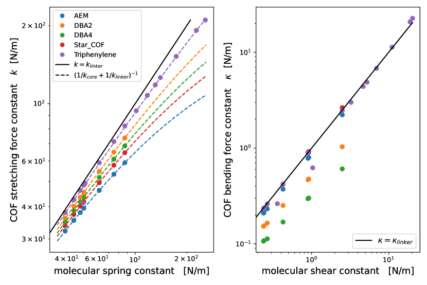
Figure 5: COF force constants vs molecular force constants for stretching (left) and bending (right). The solid lines indicates a perfect agreement. The dashed lines in the left panel are obtained by fitting Eq. (2co) to the data for each core.

4.3 Deformation energy of defective COFs

In order to assess the transferability of the models put forward in Secs. 2.1 and 2.3 to other situations, we considered COFs with a single Stone-Wales defect. We chose this type of defect, since the number of atoms remains unchanged, which facilitates the calculation of the deformation energy. For the latter we optimized the geometry of the structures without and with defect and subtract the respective energies, i.e. $E_{\rm def}=E_{\rm SW}-E_{\rm clean}$. Additionally, we minimized the energies given by Eqs. (1) and (2cm) using the effective stretching and bending force constants, $k$ and $\kappa$, and the lattice constant $a$ obtained from the DFTB results (table 1).

Figure 6 shows a Tp–DB 1phenyl–COF with a Stone-Wales defect. The atomistic structure is schematically shown by black lines and the simulation cell is indicated by grey lines. The deformation energy in DFTB is found to be $E_{\rm def}=12.66$ eV. This value is in close agreement with the values found by the model calculations which yield $E_{\rm def}=11.45$ eV (Mikado) and $E_{\rm def}=12.75$ eV (BAFF), respectively. The optimized positions of the core centers are indicated by red dots. The overall structure is well described by both coarse-grain models as indicated by a root-mean-square deviation of less than $0.5$ Ångstrom between the core-center coordinates of the models and the DFTB structure. The Mikado model is also able to capture the orientation of the cores and can thus provide information about the shape of the linkers.

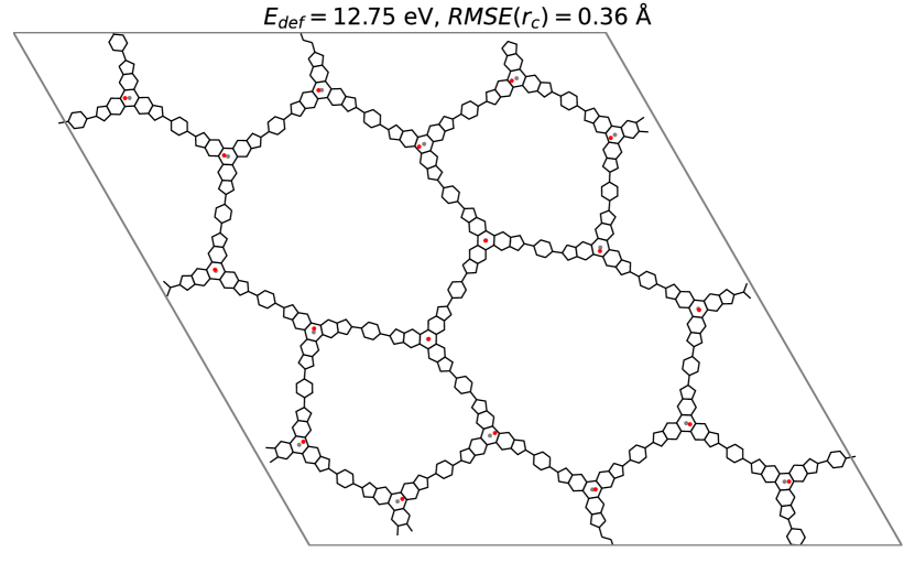
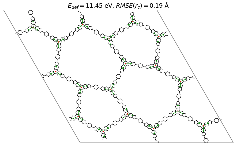
Figure 6: Stone-Wales defect in a Tp–DB 1phenyl–COF. (top) Optimized geometry obtained from DFTB (black lines) and positions of cores from BAFF (red dots). (bottom) Optimized geometry obtained from DFTB (black lines) and positions of cores from the Mikado model (red dots). The green arrows indicate the orientation of the cores.

The same procedure was repeated for the same linker but two other cores which are less rigid. Specifically, we used a Star-COF and a DBA2-COF with Stone-Wales defects (see supporting information). The deformation energies for the former COF are $E_{\rm def}^{\rm Star}=24.06$ eV (DFTB), $E_{\rm def}^{\rm Star}=19.8$ eV (Mikado), and $E_{\rm def}^{\rm Star}=22.25$ eV (BAFF). For the latter COF we obtain $E_{\rm def}^{\rm DBA2}=11.27$ eV (DFTB), $E_{\rm def}^{\rm DBA2}=7.32$ eV (Mikado), and $E_{\rm def}^{\rm DBA2}=8.02$ eV (BAFF). As one can see, the deformation energy is always underestimated by both models. The biggest difference to the DFTB results is found for the DBA2 COF, which has the smallest shear modulus of the three frameworks. The deformation energies in the Mikado model show the largest deviations from the DFTB results, but at the same time lead to structures with less deviation of the core positions.

5 Conclusions

In summary, we have calculated the in-plane elasticity of different 2D COFs with honeycomb topologies. We used DFTB to obtain the 2D bulk and shear moduli for each structure and found that both quantities decrease with increasing lattice constant. Converting the elastic constants to bond-stretching and angle-bending force-constants of a coarse-grained model, we found that the bond-stretching constants are inversely proportional to the length of the linkers, $\ell_{0}^{-1}$, while the angle-bending constants decrease as $\ell_{0}^{-3}$ or $\ell_{0}^{-4}$. These findings can be reproduced by modelling the individual linker molecules as 2D elastic beams like in the Mikado model. We computed the corresponding stretching and shear force-constants of the linker molecules and found a very good agreement with the COF force-constants for COFs with stiff cores. The elastic properties of the COFs can thus be predicted from the molecular building blocks. Moreover, the coarse-grained description can be used to investigate structures and phenomena on larger length-scales. As a demonstration, we considered three COFs with a Stone-Wales defect and compared the structure and deformation energy obtained within the coarse-grain models with the DFTB results. We find an overall good agreement, although the deformation energy is typically underestimated by the models.

It should be noted, that for a complete description of the elasticity of COFs additional information about the out-of-plane bending is required. For systems with many atoms in the unit-cell, the reliable calculation of the associated bending rigidities is quite challenging [48]. However, the coarse-graining approach presented here can also be applied in that case. Having the possibility to quantitatively relate the molecular properties of the building-blocks to the elastic properties of the COFs will facilitate the design and synthesis of 2D COFs with tailored properties.

References

- [1] Li X, Yadav P and Loh K P 2020 Chem. Soc. Rev. 49(14) 4835–4866 URL http://dx.doi.org/10.1039/D0CS00236D
- [2] Rodríguez-San-Miguel D, Montoro C and Zamora F 2020 Chem. Soc. Rev. 49(8) 2291–2302 URL http://dx.doi.org/10.1039/C9CS00890J
- [3] Colson J W and Dichtel W R 2013 Nature Chemistry 5 453–465 URL https://doi.org/10.1038/nchem.1628
- [4] Diercks C S and Yaghi O M 2017 Science 355 eaal1585 URL https://doi.org/10.1126/science.aal1585
- [5] Kim S and Choi H C 2020 ACS Omega 5 948–958 (Preprint https://doi.org/10.1021/acsomega.9b03549) URL https://doi.org/10.1021/acsomega.9b03549
- [6] Jiang D 2020 Chem 6 2461–2483 ISSN 2451-9294
- [7] Ding S Y and Wang W 2013 Chem. Soc. Rev. 42(2) 548–568 URL http://dx.doi.org/10.1039/C2CS35072F
- [8] Zwaneveld N A A, Pawlak R, Abel M, Catalin D, Gigmes D, Bertin D and Porte L 2008 Journal of the American Chemical Society 130 6678–6679 pMID: 18444643 (Preprint https://doi.org/10.1021/ja800906f) URL https://doi.org/10.1021/ja800906f
- [9] Dienstmaier J F, Gigler A M, Goetz A J, Knochel P, Bein T, Lyapin A, Reichlmaier S, Heckl W M and Lackinger M 2011 ACS Nano 5 9737–9745 pMID: 22040355 (Preprint https://doi.org/10.1021/nn2032616) URL https://doi.org/10.1021/nn2032616
- [10] Ortega-Guerrero A, Sahabudeen H, Croy A, Dianat A, Dong R, Feng X and Cuniberti G 2021 ACS Applied Materials & Interfaces 13 26411–26420 pMID: 34034486 (Preprint https://doi.org/10.1021/acsami.1c05967) URL https://doi.org/10.1021/acsami.1c05967
- [11] Wang M, Ballabio M, Wang M, Lin H H, Biswal B P, Han X, Paasch S, Brunner E, Liu P, Chen M, Bonn M, Heine T, Zhou S, Cánovas E, Dong R and Feng X 2019 Journal of the American Chemical Society 141 16810–16816 pMID: 31557002 (Preprint https://doi.org/10.1021/jacs.9b07644) URL https://doi.org/10.1021/jacs.9b07644
- [12] Sahabudeen H, Qi H, Glatz B A, Tranca D, Dong R, Hou Y, Zhang T, Kuttner C, Lehnert T, Seifert G, Kaiser U, Fery A, Zheng Z and Feng X 2016 Nature Communications 7 13461 URL https://doi.org/10.1038/ncomms13461
- [13] Dai W, Shao F, Szczerbiński J, McCaffrey R, Zenobi R, Jin Y, Schlüter A D and Zhang W 2016 Angewandte Chemie International Edition 55 213–217 (Preprint https://onlinelibrary.wiley.com/doi/pdf/10.1002/anie.201508473) URL https://onlinelibrary.wiley.com/doi/abs/10.1002/anie.201508473
- [14] Dong R, Zhang T and Feng X 2018 Chemical Reviews 118 6189–6235 pMID: 29912554 (Preprint https://doi.org/10.1021/acs.chemrev.8b00056) URL https://doi.org/10.1021/acs.chemrev.8b00056
- [15] Shao F, Dai W, Zhang Y, Zhang W, Schlüter A D and Zenobi R 2018 ACS Nano 12 5021–5029 pMID: 29659244 (Preprint https://doi.org/10.1021/acsnano.8b02513) URL https://doi.org/10.1021/acsnano.8b02513
- [16] Zhang T, Qi H, Liao Z, Horev Y D, Panes-Ruiz L A, Petkov P S, Zhang Z, Shivhare R, Zhang P, Liu K, Bezugly V, Liu S, Zheng Z, Mannsfeld S, Heine T, Cuniberti G, Haick H, Zschech E, Kaiser U, Dong R and Feng X 2019 Nature Communications 10 1–9 ISSN 20411723 URL http://dx.doi.org/10.1038/s41467-019-11921-3
- [17] Liu K, Qi H, Dong R, Shivhare R, Addicoat M, Zhang T, Sahabudeen H, Heine T, Mannsfeld S, Kaiser U, Zheng Z and Feng X 2019 Nature Chemistry 11 994–1000 ISSN 17554349 URL http://dx.doi.org/10.1038/s41557-019-0327-5
- [18] Zeng Y, Gordiichuk P, Ichihara T, Zhang G, Sandoz-Rosado E, Wetzel E D, Tresback J, Yang J, Kozawa D, Yang Z, Kuehne M, Quien M, Yuan Z, Gong X, He G, Lundberg D J, Liu P, Liu A T, Yang J F, Kulik H J and Strano M S 2022 Nature 602 91–95 URL https://doi.org/10.1038/s41586-021-04296-3
- [19] Zhou W, Wu H and Yildirim T 2010 Chemical Physics Letters 499 103–107 URL https://doi.org/10.1016/j.cplett.2010.09.032
- [20] Duong L N, Tuoc V N and Thao N T 2019 Journal of Physics: Conference Series 1274 012010 URL https://doi.org/10.1088/1742-6596/1274/1/012010
- [21] Ziogos O G, Blanco I and Blumberger J 2020 The Journal of Chemical Physics 153 044702 URL https://doi.org/10.1063/5.0010164
- [22] Xu L, Zhou X, Tian W Q, Gao T, Zhang Y F, Lei S and Liu Z F 2014 Angewandte Chemie International Edition 53 9564–9568 (Preprint https://onlinelibrary.wiley.com/doi/pdf/10.1002/anie.201400273) URL https://onlinelibrary.wiley.com/doi/abs/10.1002/anie.201400273
- [23] Qi H, Sahabudeen H, Liang B, PoloÅŸij M, Addicoat M A, Gorelik T E, Hambsch M, Mundszinger M, Park S, Lotsch B V, Mannsfeld S C B, Zheng Z, Dong R, Heine T, Feng X and Kaiser U 2020 Science Advances 6 eabb5976
- [24] Castano I, Evans A M, Reis R d, Dravid V P, Gianneschi N C and Dichtel W R 2021 Chemistry of Materials 33 1341–1352
- [25] Raptakis A, Dianat A, Croy A and Cuniberti G 2021 Nanoscale 13(2) 1077–1085 URL http://dx.doi.org/10.1039/D0NR07666J
- [26] Landau L D and Lifshitz E M 1986 Theory of elasticity 3rd ed (Oxford: Butterworth-Heinemann)
- [27] Wilhelm J and Frey E 2003 Phys. Rev. Lett. 91(10) 108103 URL https://link.aps.org/doi/10.1103/PhysRevLett.91.108103
- [28] Head D A, Levine A J and MacKintosh F C 2003 Phys. Rev. Lett. 91(10) 108102 URL https://link.aps.org/doi/10.1103/PhysRevLett.91.108102
- [29] Lagnese J E, Leugering G and Schmidt E J P G 1993 Mathematical Methods in the Applied Sciences 16 327–358
- [30] Phani A S, Woodhouse J and Fleck N A 2006 The Journal of the Acoustical Society of America 119 1995–2005
- [31] Elstner M, Porezag D, Jungnickel G, Elsner J, Haugk M, Frauenheim T, Suhai S and Seifert G 1998 Phys. Rev. B 58 7260–7268
- [32] Elstner M 2007 J. Phys. Chem. A 111(26) 5614–5621
- [33] Stone A and Wales D 1986 Chemical Physics Letters 128 501–503 ISSN 0009-2614 URL https://www.sciencedirect.com/science/article/pii/0009261486806613
- [34] Ockwig N W, Co A P, Keeffe M O, Matzger A J and Yaghi O M 2005 Science 310 1166–1171 URL https://science.sciencemag.org/content/310/5751/1166
- [35] Feng X, Dong Y and Jiang D 2013 CrystEngComm 15(8) 1508–1511 URL http://dx.doi.org/10.1039/C2CE26371H
- [36] Baldwin L A, Crowe J W, Shannon M D, Jaroniec C P and McGrier P L 2015 Chemistry of Materials 27 6169–6172 (Preprint https://doi.org/10.1021/acs.chemmater.5b02053) URL https://doi.org/10.1021/acs.chemmater.5b02053
- [37] Yang H, Du Y, Wan S, Trahan G D, Jin Y and Zhang W 2015 Chem. Sci. 6(7) 4049–4053 URL http://dx.doi.org/10.1039/C5SC00894H
- [38] Côté A P, El-Kaderi H M, Furukawa H, Hunt J R and Yaghi O M 2007 Journal of the American Chemical Society 129 12914–12915 pMID: 17918943 (Preprint https://doi.org/10.1021/ja0751781) URL https://doi.org/10.1021/ja0751781
- [39] Rager S, Dogru M, Werner V, Gavryushin A, Götz M, Engelke H, Medina D D, Knochel P and Bein T 2017 CrystEngComm 19(33) 4886–4891 URL http://dx.doi.org/10.1039/C7CE00684E
- [40] Kou Y, Xu Y, Guo Z and Jiang D 2011 Angewandte Chemie International Edition 50 8753–8757
- [41] Pham H Q, Le D Q, Pham-Tran N N, Kawazoe Y and Nguyen-Manh D 2019 RSC Adv. 9(50) 29440–29447 URL http://dx.doi.org/10.1039/C9RA05159G
- [42] Guo J, Xu Y, Jin S, Chen L, Kaji T, Honsho Y, Addicoat M A, Kim J, Saeki A, Ihee H, Seki S, Irle S, Hiramoto M, Gao J and Jiang D 2013 Nature Communications 4 2736 URL https://doi.org/10.1038/ncomms3736
- [43] Perebeinos V and Tersoff J 2009 Phys. Rev. B 79 241409
- [44] Head D A, Levine A J and MacKintosh F C 2003 Phys. Rev. E 68(6) 061907 URL https://link.aps.org/doi/10.1103/PhysRevE.68.061907
- [45] Lukose B, Kuc A, Frenzel J and Heine T 2010 Beilstein J. Nanotechnol. 1 3762
- [46] Monkhorst H J and Pack J D 1976 Phys. Rev. B 13(12) 5188–5192 URL https://link.aps.org/doi/10.1103/PhysRevB.13.5188
- [47] Haastrup S, Strange M, Pandey M, Deilmann T, Schmidt P S, Hinsche N F, Gjerding M N, Torelli D, Larsen P M, Riis-Jensen A C, Gath J, Jacobsen K W, Mortensen J J, Olsen T and Thygesen K S 2018 2D Materials 5 042002 URL https://doi.org/10.1088/2053-1583/aacfc1
- [48] Kumar S and Suryanarayana P 2020 Nanotechnology 31 43LT01 URL https://doi.org/10.1088/1361-6528/aba2a2