Verification of Sigmoidal Artificial Neural Networks using iSAT

Abstract

This paper presents an approach for verifying the behaviour of nonlinear Artificial Neural Networks (ANNs) found in cyber-physical safety-critical systems. We implement a dedicated interval constraint propagator for the sigmoid function into the SMT solver iSAT and compare this approach with a compositional approach encoding the sigmoid function by basic arithmetic features available in iSAT and an approximating approach. Our experimental results show that the dedicated and the compositional approach clearly outperform the approximating approach. Throughout all our benchmarks, the dedicated approach showed an equal or better performance compared to the compositional approach.

This work has received funding from the German Federal Ministry of Economic Affairs and Climate Action (BMWK) through the KI-Wissen project under grant agreement No. 19A20020M, and from the State of Lower Saxony within the framework “Zukunftslabor Mobilität Niedersachsen” (https://www.zdin.de/zukunftslabore/mobilitaet).

1 Introduction

In the age of highly automated systems and the development of autonomous systems, a possible application scenario for ANNs is to use them as controllers for safety-critical cyber-physical systems (CPSes) [10]. Such CPSes capture the often complex environment, analyse the data and make control decisions about the future system behaviour. Guarantees on compliance with safety requirements, e.g., that human lives are not endangered, are of utmost importance. Whenever such guarantees are obtained via formal verification of the system behaviour, an ANN being a component of the system under analysis has also to be subject to verification [24].

The underlying weighted summation of the input neurons before application of the activation function can be represented by simple linear combinations and is therefore very appealing for classical verification methods dealing with linear arithmetic. However, this observation is deceptive when nonlinear activation functions are part of the ANN as such nonlinear functions are often hard to analyse in themselves [24]. Apart from restricted decidability results for reachability problems as in [10], the runtime of algorithms for automatic verification suffers from the multiple occurrence of nonlinear activation functions in complex ANNs such that only relatively small networks could be tackled. Depending on the class of activation functions and the underlying possibly necessary abstractions thereof, recent approaches were able to deal with ANNs comprising 20 to 300 nodes [11, 19, 20].

So-called satisfiability modulo theory (SMT) solvers implement algorithms that search for solutions to Boolean combinations of arithmetic constraints or prove the absence thereof. Such SMT solvers are often used for automatic verification of safety-critical properties in CPSes [22, 11]. Here, a symbolic description of the possible system behaviour in terms of a constraint system is analysed for the existence of a system run reaching a state violating a safety requirement. In order to apply automatic verification to ANNs with nonlinear activation functions, which is necessary for automatic verification of CPSes comprising such ANNs, the SMT solver used must support the corresponding class of arithmetic.

The SMT solver iSAT [5, 8] solver reasons over the — in general undecidable — theory of Boolean combinations of nonlinear arithmetic constraints. It tightly couples the well-known Boolean decision procedure DPLL [4] with interval constraint propagation (ICP) [21] for real arithmetic. In addition to basic arithmetic operations, iSAT also supports nonlinear and transcendental operators. Given an input formula and interval bounds of the real-valued variables, iSAT searches for a satisfiable solution within the interval bounds. The iSAT algorithm incorporates an alternation of deduction and decision steps. A decision step selects a variable, splits its current interval and decides for one of the resulting intervals to be the search space of the variable in the further course of the search. A deduction step then applies forward and backward interval constraint propagation until either a fixed point is reached, or an empty interval is derived which means that the formula is unsatisfiable under the current assumptions (decisions). The latter result causes a revoke of deductions of interval bounds and a reversal of decisions which yields, if possible, a decision for a yet unexplored part of the search space. If no decision for an unexplored part of the search space is possible, the formula is proven to be unsatisfiable under the initial assumption of the bounds on the search space.

Due to the inherent availability of nonlinear operators, iSAT seems to be a promising tool for verification of ANNs employing nonlinear activation functions. ANNs such as Deep Learning (DL) architectures make use of the nonlinear and transcendental sigmoid function (and their evolved variations) in hidden and output layers [23]. Although the solver iSAT can already represent the sigmoid function by a composition of existing propagators, this paper pursues the hypothesis that for nonlinear functions, a propagator which can exactly propagate the function in once (in following called dedicated propagator) is preferable. For the investigation of this hypothesis, the sigmoid function is used in this paper. We therefore present an approach for verifying sigmoidal ANNs based on a dedicated interval constraint propagator for the sigmoid function integrated into iSAT. In our experiments, we demonstrate based on runtime comparisons that our approach points into a promising direction for future research on the verification of nonlinear ANNs.

The paper is organised as follows. In Sec. 2, we present the related work regarding different approaches for verifying ANNs. Sec. 3 details the proposed approach for verifying ANNs using the iSAT solver and is divided into several parts. We first discuss and compare different encoding schemes for the sigmoid activation function (Sec. 3.1), present our experimental setup (Sec. 3.2), and present some preliminary results regarding the encoding schemes (Sec. 3.3). Afterwards, we report on improvements in the preprocessing step of iSAT (Sec. 3.4) that proved helpful for the following verification of severe safety properties that is discussed in Sec. 3.5. Finally, in Sec. 4 we present the conclusions and future work of this paper.

2 Related Work

In the literature, there is a high research interest regarding the verification of ANNs, especially regarding cyber-physical safety-critical systems.

The authors in [19] present an approach that verifies the safety of a fully connected feedforward network and applies automatic corrections to the neurons. For this purpose, an industrial manipulator with its kinematic properties was used as a physical system. More exactly, an ANN with the sigmoid function being used as an activation function was used to predict the final position depending on the given joint angles of the industrial manipulator. The presented approach deals with an abstraction of the concrete ANN, were the the abstraction domain was chosen to be the set of (closed) intervals of real numbers. The corresponding abstraction of the sigmoid activation function is hence given by piecewise interval boxes of fixed width that encapsulate the concrete function. The chosen abstraction is consistent, i.e, if the abstraction of a safety property is valid in the abstract domain, then it must hold also for the concrete domain. The verification task could be handled by the SMT solver HySAT. When HySAT produces an abstract counterexample, it has to be analysed whether it has a concretisation or is spurious. In the later case, a refinement of the interval boxes is triggered. In addition, the authors propose to use spurious counterexamples for a ’repair’ of the ANN, i.e., they propose to add a correct labelled concretisation to the training set for later trainings. The corresponding tool is called NeVer.

In 2017, the authors in [11] from Stanford University published the algorithm Reluplex. Reluplex is based on the well-known Simplex algorithm for linear programming. The idea of Reluplex is to extend the simplex algorithm with new rules for the piecewise linear ReLU-activation function (Rectified Linear Unit). The task was to verify a prototypical DNN implementation of the new collision avoidance system ACAS Xu [17] for unmanned aerial vehicles (UAVs). The deep neural networks (fully connected and feed-forward) were trained on a look-up table that holds information about which manoeuvre advisories are to be executed next depending on seven input parameters. The evaluation was performed on 45 networks with 300 hidden neurons each, where the Reluplex algorithm was able to prove (and disprove) that certain safety-critical properties hold for the given DNN. Furthermore, the robustness of the deep neural network system was tested. It was possible to determine individual input neurons and their sensitivity to perturbations by adding a perturbation factor to the input and checking the output [11].

The Reluplex approach has been included into the Marabou framework [12] in 2019. Marabou works with ANNs using arbitrary piecewise-linear activation functions and follows the spirit of Reluplex as it uses a lazy SMT-technique that postpones a case-split of nonlinear constraints as far as possible, in the hope that many of them prove irrelevant for the property under investigation.

Also in 2017, another approach to verification of deep neural networks was published in [9]. Here, the safety analysis of classification decisions is driven by so-called adversarials. For a given input vector $x$, the invariance of the classification decision of the deep neural network is to be proven or disproven layer by layer by considering disturbances or manipulations within a region around the layer’s activation. Hence, a deep neural network is safe if, for a given input vector and region, the application of specific manipulations does not lead to a change in the classification decision. Such a region can be spanned manually or automatically, by taking a hyperrectangle around the activation. The hyperrectangle has a nontrivial extent in a given number of dimensions, these being the dimensions where the activation value is furthest away from the average activation value of the layer. Manipulations for the selected region can also be determined manually or by adding or subtracting a small numerical value (so-called small span) depending on the positive or negative deviation of the average activation. After the selection of the region and the manipulations, the SMT Solver Z3 is used to check whether a misclassification is already possible in the considered layer due to the applied manipulations compared to the input. If there is no misclassification, an automatic determination of the region and manipulations in the next layer depends on the region and manipulations of the previously considered layer. In order to automatically find valid manipulations, the solver Z3 is also used. Thus, a safety statement can be made whether the classification network is robust on the specific input against perturbations within the initially specified region or not. Focusing on classification problems, evaluations on image classification deep neural networks were performed in this publication. These include a neural network for handwritten digit recognition (greyscale) based on the MNIST data-set [16], CIFAR-10 for object recognition [14], and ImageNet [15] for 3-channel colour images [9]. The evaluation showed that the approach scales well in terms of neural network size (state-of-the-art 16-layers image classification networks) and the amount of total parameters (up to 138,357,544 in experiments) since each layer is checked individually for misclassifications. Unfortunately, no temporal information was provided for the performed experiments. A statement about the safety of a neural network is made by falsification. If no misclassification was found, the network is safe considering the specific vector, the selected region, and the set of manipulations. The evaluation was done with the solver Z3 [18, 9].

In 2018, the authors of [7] presented the verification of safety and robustness properties of feed-forward neural networks with max-pooling layers as well as convolutional neural networks. The presented approach uses the classical framework of abstract interpretation to overapproximate the behaviour of the original neural network. For the approximation the authors investigated different domains of polyhedral shapes, e.g., boxes, zonotopes (restricted class of point-symmetrical polyhedra) and general convex polyhedra. The approach was evaluated on fully-connected feedforward neural networks with ReLU-function as activation function trained with the MNIST [16] and CIFAR [14] data-set. The results have shown better scalability and precision on state-of-the-art neural networks compared to Reluplex [11]. The state-of-the-art neural network analyser ERAN [2] subsumes the presented approach.

In this work, we present the approach of verifying fully connected feedforward neural networks containing sigmoid activation functions using the SMT solver iSAT [5] that builds on interval constraint propagation and supports nonlinear and transcendental arithmetic.

3 Verifying Sigmoidal ANNs with iSAT

In this section, we present our approach regarding verification of ANNs using the SMT solver iSAT. In Sec. 3.1 we specify how the ANNs and their desired safety properties are encoded into iSAT. We describe three different approaches to encode the sigmoid function into iSAT. In Sec. 3.2 we introduce our benchmark set including the used verification targets. A mild subset of the verification targets was used for a first comparison of the encoding approaches as presented in Sec. 3.3. As in this early phase of our investigation it turned out already, that iSAT has some runtime issues with regard to the preprocessing of the input formula, we report on our countermeasures to improvements the preprocessing in Sec. 3.4. Finally, in Sec. 3.5 we report on our experience on safety verification using a subset of severe verification targets.

3.1 Translating ANN into iSAT

Safety Properties

An ANN encodes a functional relation $o=F(i)$ between the network input $i$ and the network output $o$. Since all edges between neurons, weights and transfer functions are known for a trained network, this information can be extracted, and $F$ can be written as a comprehensive arithmetic expression, and hence fed into the SMT solver iSAT. A safety property for the ANN relates input constrains $\Phi(i)$ with output constraints $\Psi(o)$ — both given again as arithmetic expressions — , and we say that the ANN satisfies the safety property if and only if the implication $(o=F(i)\land\Phi(i))\to\Psi(o)$ holds for all inputs $i$ and outputs $o$. That is, whenever iSAT certifies that the negation of the safety property, $o=F(i)\land\Phi(i)\land\lnot\Psi(o)$, is unsatisfiable, we have proven the safety property for the ANN. On the other hand, if iSAT provides a solution to the given problem it found a counterexample for the desired property. Often, iSAT provides a so-called candidate solution only. A candidate solution specifies for each solver variable an interval in which a possible solution could be found. Such a candidate solution needs to be analysed in subsequent steps.

Sigmoid as Activation Function

As already said in the introduction we aim at the verification of ANNs using the sigmoid function

$$sig(x):\mathbb{R}\to(0,1)\;\text{, }\;\;x\mapsto\frac{1}{1+\mathrm{e}^{-x}}\;\text{, }\;\;$$ (1)

as activation function, and compare different encoding approaches of the sigmoid function into iSAT.

Figure 1: The graph of the sigmoid function $y=\operatorname{sig}(x)$.

Figure 2: Approximation of $y=\operatorname{sig}(x)$ by encapsulating interval boxes.

Figure 3: Interval constraint propagation for $\operatorname{sig}(x)$. $X^{\prime}$ and $Y^{\prime}$ are the smallest intervals that still contain all solutions of $y=\operatorname{sig}(x)$ that were previously in $X$ and $Y$.

iSAT Encoding Approaches

In a first step, we were mainly interested in a comparison of different approaches for the arithmetic encoding of the functional relation $o=F(i)$ with regard to the sigmoid activation function.

1. As iSAT provides the necessary arithmetic means to express $\operatorname{sig}(x)$ as a composition of basic arithmetic operations and the exponential function as indicated on the right hand side of Eq. 1, this yields the canonical compositional approach.

2. Since we assumed that a specialised propagator for sigmoid would behave better for the verification task, we built such an specialised propagator into iSAT, which led to the dedicated approach.

3. Finally, we were also interested in an approximating approach that uses — similar to the sigmoid abstraction in [19] — a piecewise interval encapsulation of the sigmoid function, cf. Fig. 3. Within the domain interval $[-8,8)$ we encapsulated the sigmoid function in interval boxes of a fixed width $p=0.5$ and for the remaining $x$-values below $-8$ and above $8$ we used unbounded interval boxes. Hence, we replaced any occurrence of the relation $y=\operatorname{sig}(x)$ by the formula

   $$\Big{(}x\in\big{(}-\infty,8\big{)}\,\to\,y\in\big{[}0,\operatorname{sig}(-8)\big{)}\Big{)}\land\Big{(}x\in\big{[}-8,-7.5\big{)}\,\to\,y\in\big{[}\operatorname{sig}(-8),\operatorname{sig}(-7.5)\big{)}\Big{)}\land\dots$$

   $$\dots\land\Big{(}x\in\big{[}7.5,8.0\big{)}\,\to\,y\in\big{[}\operatorname{sig}(7.5),\operatorname{sig}(8)\big{)}\Big{)}\land\Big{(}x\in\big{[}8,+\infty\big{)}\,\to\,y\in\big{[}\operatorname{sig}(8),1\big{]}\Big{)}.$$

   The intention behind this approach was to find out whether such an approximation could have a positive effect on the running times of iSAT.

Dedicated Propagator

We shortly discuss the theoretical background of the sigmoid propagator and describe how we implemented this propagator into iSAT. For the general approach to implement arbitrary propagators into iSAT, the interested reader is referred to [8, Ch. 5]. Let $f:\mathbb{R}\to\mathbb{R}$ be a function and $\mathbb{I}$ be the set of real-valued intervals. Further, let $y=f(x)$ be an equation relating two variables $x\in X$ and $y\in Y$ with $X,Y\in\mathbb{I}$. An interval constraint propagator $\rho_{f}:\mathbb{I}^{2}\to\mathbb{I}^{2}$ for $f$ maps $X\times Y$ to the smallest subset $X^{\prime}\times Y^{\prime}$ in $X\times Y$ that contains all solutions to ${y=f(x)}$ that have been in $X\times Y$, i.e. $\forall(x,y)\models y=f(x)$ we have $(x,y)\in X\times Y\implies(x,y)\in X^{\prime}\times Y^{\prime}$. Such a propagator thus chops parts from $X$ and $Y$ for which no solution to $y=f(x)$ exists, cf. Fig. 3.

Since $\operatorname{sig}(x)$ is continuous and strictly monotonic increasing, the boundary values of $X^{\prime}$ and $Y^{\prime}$ can be deduced directly from the boundary values of $X$ and $Y$ by applying $\operatorname{sig}(x)$ and its inverse $\operatorname{sig}^{-1}(x)$. The cases that $X$ is not bounded or that the bounds of $Y$ are not in the domain of $\operatorname{sig}(x)$ are special. In order to cover these cases, we lift $\operatorname{sig}(x)$ and $\operatorname{sig}^{-1}(x)$ to the extended field of real numbers $\overline{\mathbb{R}}=\mathbb{R}\cup\{{-\infty,\infty}\}$ by defining two functions $\sigma:\overline{\mathbb{R}}\to\overline{\mathbb{R}}$ and $\sigma^{-1}:\overline{\mathbb{R}}\to\overline{\mathbb{R}}$ as

$$\begin{aligned} \sigma(x):=\begin{cases}0&\text{ if }x={-\infty}\\ \frac{1}{1+\mathrm{e}^{-x}}&\text{ if }{-\infty}<x<\infty\\ 1&\text{ if }x=+\infty,\\ \end{cases}\end{aligned}\qquad\begin{aligned} \sigma^{-1}(y):=\begin{cases}-\infty&\text{ if }y\leq 0\\ -\ln(\frac{1}{y}-1))&\text{ if }0<y<1\\ +\infty&\text{ if }1\leq y.\end{cases}\end{aligned}$$

The interval constraint propagation for the sigmoid function is implemented in iSAT as two functions representing the so-called forward propagation that yields $Y^{\prime}$, and the backward propagation that yields $X^{\prime}$. The corresponding algorithms $\mathsf{fwd\_prop}_{\sigma}(X,Y)$ and $\mathsf{bwd\_prop}_{\sigma}(X,Y)$ are listed in Alg. 1 and Alg. 2 where $({\bowtie}_{1},x_{1},{\bowtie}_{2},x_{2})$ with $x_{1},x_{2}\in\overline{\mathbb{R}}$ and ${\bowtie}_{1},{\bowtie}_{2}\in\{{<},{\leq}\}$ represents an interval $I=\{x\mid x_{1}\bowtie_{1}x\bowtie_{2}x_{2}\}$. Please note that the floor and ceiling notations $\lfloor\,\rfloor$ and $\lceil\,\rceil$ here refer to a rounding towards the next floating point number available on the computer on which iSAT is executed. Rounding of boundary values is required since the finite precision of machine-representable numbers does not allow to represent arbitrary real values. However, such safe outward rounding guarantees that all solutions to $y=\operatorname{sig}(x)$ from $X\times Y$ are included in $X^{\prime}\times Y^{\prime}$.

Input: $X=({\bowtie}_{1},x_{1},{\bowtie}_{2},x_{2})$, $Y$

$y_{1}:=\lfloor\sigma(x_{1})\rfloor$;

$y_{2}:=\lceil\sigma(x_{2})\rceil$;

${\bowtie}_{1}^{\prime}:={\bowtie}_{1}$;

${\bowtie}_{2}^{\prime}:={\bowtie}_{2}$;

if  $y_{1}=-\infty$  then ${\bowtie}_{1}^{\prime}:={<}$;

if  $y_{2}=+\infty$  then ${\bowtie}_{2}^{\prime}:={<}$;

$Y^{\prime}:=Y\cap(\bowtie_{1}^{\prime},y_{1},\bowtie_{2}^{\prime},y_{2})$;

return $Y^{\prime}$;

Algorithm 1 $\mathsf{fwd\_prop}_{\sigma}(X,Y)$

Input: $X$, $Y=({\bowtie}_{1},y_{1},{\bowtie}_{2},y_{2})$

$x_{1}:=\lfloor\sigma^{-1}(y_{1})\rfloor$;

$x_{2}:=\lceil\sigma^{-1}(y_{2})\rceil$;

${\bowtie}_{1}^{\prime}:={\bowtie}_{1}$;

${\bowtie}_{2}^{\prime}:={\bowtie}_{2}$;

if  $x_{1}=0$  then ${\bowtie}_{1}^{\prime}:={<}$;

if  $x_{2}=1$  then ${\bowtie}_{2}^{\prime}:={<}$;

$X^{\prime}:=X\cap(\bowtie_{1}^{\prime},x_{1},\bowtie_{2}^{\prime},x_{2})$;

return $X^{\prime}$;

Algorithm 2 $\mathsf{bwd\_prop}_{\sigma}(X,Y)$

Such a dedicated propagator allows to encode a sigmoidal ANN directly into iSAT without any paraphrasing through composition of functions. In addition, the direct encoding involves only one operator per sigmoidal activation and thus a single propagator call; the compositional approach instead requires multiple propagator calls, namely one for each arithmetic function used in the encoding. We thus expect the dedicated propagator to outperform the compositional approach.

3.2 Experimental Setup

We describe the networks and applications we used to compare the approaches. We trained various networks for two applications, namely a) to give an emergency brake advisory within a train control system, and b) to recognise hand-written digits.

We performed two types of evaluation on these networks. Based on the train control example, we compared the runtime performance of the dedicated propagator to the compositional and the approximating approach, the results are presented in Sec. 3.3. In Sec. 3.5, we aimed at a more severe verification task using dedicated safety properties. We performed corresponding benchmarks based on the digit recognition example as well as on the train control example. For all these benchmarks, we translated ONNX [6] models of our trained networks into an SMT formula in the iSAT language which then was extended by additional constraints specifying the property to verify.

The remainder of this section describes the two applications, the networks we trained for our benchmarks, and the properties we tried to verify.

3.2.1 European Train Control System (ETCS)

One of the applications used for our evaluation is a simplified emergency brake advisory function from the moving block authority of the European Train Control System according to [8]: Two trains are running behind each other on one track into the same direction (see Fig. 4). The train behind shall be advised to initiate an emergency braking manoeuvre if it cannot stop without violating a safety distance to the train ahead, i.e. the distance to the train ahead is smaller than the minimum braking distance (using maximum deceleration) plus a safety distance. We consider the worst case scenario where the train ahead is at standstill.

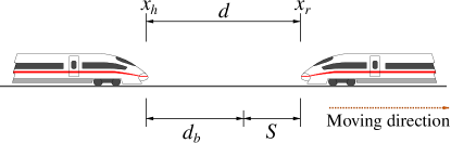
Figure 4: Simplified European Train Control System (ETCS) model

We assume that the maximum deceleration for the train behind is $-0.7\text{\,}\mathrm{m}\text{\,}{\mathrm{s}}^{-2}$ and a safety distance $S=$400\text{\,}\mathrm{m}$$. Let $x_{h}$ describe the head position of the train behind, while $x_{r}$ is the rear position of the train ahead. The maximum braking distance $d_{b}$ available before entering the safety margin to the train ahead and the deceleration $a$ required to stop with exactly the safety distance are calculated as

$$d_{b}=x_{r}-(x_{h}+S)\text{\hskip 28.45274ptand\hskip 28.45274pt}a=-\frac{v^{2}}{2d_{b}}\;,$$

where $v$ is the velocity of the train behind. The system shall then advise for an emergency brake if and only if the deceleration required to stop with exactly the safety margin is larger than the maximum deceleration, i.e.

$$\mathit{braking}\equiv\begin{cases}\text{true}&\text{if }a<$-0.7\text{\,}\mathrm{m}\text{\,}{\mathrm{s}}^{-2}$\;,\\ \text{false}&\text{otherwise.}\end{cases}$$

We used the Keras API [3] in combination with the Adam optimisation algorithm [13] to train 16 fully connected feedforward ANNs for this function, each of which varying in the number of layers, the number of neurons per layer, and the total number of neurons as illustrated in Tab. 1. Each network has three input neurons for $v$, $x_{h}$, and $x_{r}$ as well as two output neurons $\mathrm{out}_{0}$ and $\mathrm{out}_{1}$. The output value of $\mathrm{out}_{0}$ votes for “not braking” and the value of $\mathrm{out}_{1}$ votes for “braking”. The network indicates the braking advisory $\mathit{braking}\equiv\mathrm{true}$ if and only if the vote of $\mathrm{out}_{1}$ outweighs the vote of $\mathrm{out}_{0}$, i.e. if and only if $\mathrm{out}_{0}\leq\mathrm{out}_{1}$.

The training was performed based on a self-generated data set containing $200\,000$ entries. Each entry contains the velocity $v$ of the train behind, the track positions $x_{r}$ and $x_{h}$, and the braking advisory $\mathit{braking}$. The velocity may range from $0$ to $83.4\text{\,}\mathrm{m}\text{\,}{\mathrm{s}}^{-1}$, the length of the track is $50\,000\text{\,}\mathrm{m}$, and the safety distance is not violated trivially, i.e. we always have $d_{b}\geq 0$.

Table 1: Distribution of neurons in ETCS and MNIST networks (fully connected and feedforward). The neurons per hidden layer are explicitly specified per layer for the MNIST networks.

model name	input / output layer		hidden layers
	$\overbrace{\rule{91.04872pt}{0.0pt}}$		$\overbrace{\rule{187.78836pt}{0.0pt}}$
	input nodes	output nodes	no. of layers	neurons per layer	total no. of neurons
ETCS	3	2	2	12	24
	3	2	2	25	50
	3	2	2	50	100
	3	2	2	100	200
	3	2	3	12	36
	3	2	3	25	75
	3	2	3	50	150
	3	2	3	100	300
	3	2	4	12	48
	3	2	4	25	100
	3	2	4	50	200
	3	2	4	100	400
	3	2	5	12	60
	3	2	5	25	125
	3	2	5	50	250
	3	2	5	100	500
MNIST	784	10	2	(392, 196)	588
	784	10	2	(784, 392)	1 176

Properties to Verify

We used these networks for both types of evaluation: for the comparison of approaches and for the dedicated attempt to verify a property.

For the comparison of approaches, we used several verification targets, some of them expected to yield a satisfiable constraint system as well as some expected to yield an unsatisfiable constraint system, thereby aiming at a broad overview of how the approaches perform on the class of constraint systems yielded by our encoding approaches. Throughout all verification tasks, we investigated whether the advice $\mathit{braking}\equiv\mathrm{true}$, indicated by $\mathrm{out}_{0}\leq\mathrm{out}_{1}$, is satisfiable or not, i.e. we added a constraint $\mathrm{out}_{0}>\mathrm{out}_{1}$ to the iSAT input s.t. the desired property is satisfied iff the resulting constraint system is unsatisfiable. The verification tasks varied in the search space, i.e. in their constraints on the input to the ANN, as in the following scenarios:

1. We left the inputs unconstrained.

2. We restricted positions to $x_{r}>x_{h}$, i.e. to situations where there train behind runs with some positive distance behind the train ahead.

3. We restricted the train behind to a velocity $v>$25\text{\,}\mathrm{m}\text{\,}{\mathrm{s}}^{-1}$$ and the position $x_{h}=$15\,000\text{\,}\mathrm{m}$$ and the position of the train ahead was restricted to $x_{r}=$35\,000\text{\,}\mathrm{m}$$. In this scenario, the property is expected not to be satisfied.

4. Again, we restricted the train behind to a velocity $v>$25\text{\,}\mathrm{m}\text{\,}{\mathrm{s}}^{-1}$$ while the positions of both trains were constrained to ${x_{h},x_{r}<$800\text{\,}\mathrm{m}$}$. This yields only situations where violating the safety distance $S$ is unavoidable due to the limited maximum distance between the trains. Thus, the property is expected to be unsatisfied.

We applied all these variants to all ETCS networks listed in Tab. 1 for all three approaches, namely the compositional approach, the approximating approach, and the dedicated propagator.

When aiming at a severe verification task, we assumed that the velocity of the train behind is ${v\in($20\text{\,}\mathrm{m}\text{\,}{\mathrm{s}}^{-1}$,$80\text{\,}\mathrm{m}\text{\,}{\mathrm{s}}^{-1}$]}$, and that the distance $d=x_{r}-x_{h}$ between the trains is smaller than the safety margin $S$, i.e. $d\in[$0\text{\,}\mathrm{m}$,S]$. This setup inherently requires an advisory $\mathit{braking}\equiv\mathrm{true}$. We hence added the corresponding constraints on the inputs of the ANN under inspection to the iSAT input plus a constraint $\mathrm{out}_{0}>\mathrm{out}_{1}$ and aimed at a proof that the resulting constraint system is unsatisfiable, i.e. that the corresponding ANN always advised for an emergency brake when the distance between the trains is smaller than the safety margin.

3.2.2 Recognition of Handwritten Digits

We trained two fully connected feedforward networks for the recognition of handwritten digits each of them comprising two hidden layers and varying in the number of neurons per layer as well as the total number of neurons as indicated in Tab. 1.

The training was based on the MNIST data set [16] which is widely used in the context of artificial neural network classification. The data set consists of over 60.000 entries of grey-scaled images of size 28x28 pixels with each pixel value being an integer in $[0,255]$. Each image represents a handwritten digit from 0-9 (see Fig. 5).

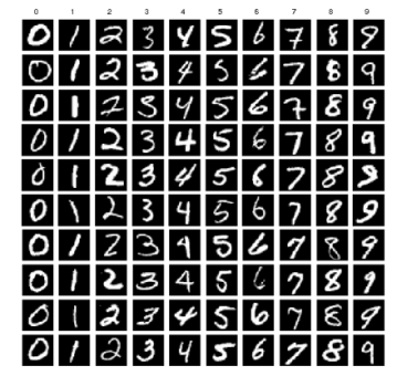
Figure 5: Handwritten digits from the MNIST data set

Property to Verify

For this benchmark we drew a number of samples from the MNIST database. We searched for counterexamples violating a property to guarantee within an $\varepsilon$-box around the sample, i.e. for any sample $s$ with vector components $s_{k}$ and $1\leq k\leq 28^{2}$, we constrained the inputs to the network within the constraint system describing the network to $\max(0,s_{k}-\varepsilon)\leq\mathrm{in}_{k}\leq\min(1,s_{k}+\varepsilon)$ with $\varepsilon=2.55$.

Let $j$ be the true digit of the sample. For each sample, we formulate the verification targets, i.e. the constraints added to the constraint system, as follows. We asked for a unique identification of $j$, i.e. we tried to prove that the output value for $\mathrm{out}_{j}$ is the largest. A counterexample to this property would thus satisfy the constraint $\bigvee_{i=0}^{9}\mathrm{out}_{i}\geq\mathrm{out}_{j}$ for $i\neq j$.

In order to alleviate the solving process, we split up this condition along the disjunction into multiple constraint systems instead of testing all outputs within a single solver run. We thus created a constraint system for each $i\neq j$ for each sample comprising a constraint $\mathrm{out}_{i}\geq\mathrm{out}_{j}$. We thus moved the disjunction of the above condition to file level, i.e. the property is not satisfied if one of those constraint systems is satisfiable. For this benchmark, we drew 20 samples, thereby yielding 180 constraint systems to solve for both digit recognition networks.

3.3 Comparison of Approaches

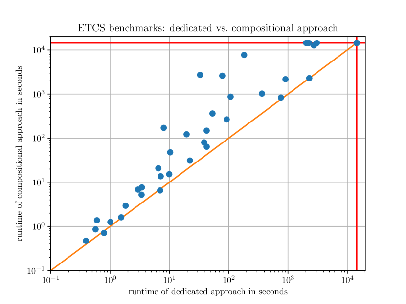
(a) Dedicated propagator vs. compositional approach

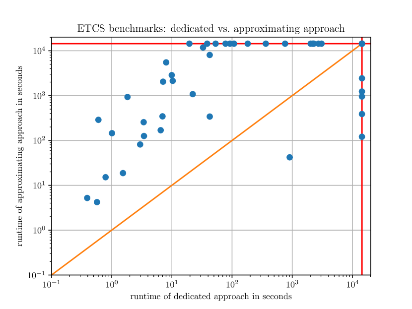
(b) Dedicated propagator vs. approximating approach

Figure 6: Comparison of the runtimes of the approach using the dedicated sigmoid propagator with the runtimes of the compositional approach (a) and the approximating approach (b). The horizontal axes show the runtimes using the dedicated propagator while vertical axes show the runtimes of the comparative approaches (all axes are in logscale). Each data point illustrates the runtimes of the compared approaches on a particular network and verification target. Timeouts are located on the red borders. The orange line indicates the line of equal runtime. The benchmarks were performed with a timeout of 4 hours (14,400 seconds).

We compare the dedicated sigmoid propagator with the compositional approach and the approximating approach based on runtime evaluations. To this end, we executed benchmarks on the ETCS networks described in Tab. 1 where we investigated whether the advice $\mathit{braking}\equiv\mathrm{true}$ is satisfiable or not in four different settings (see Sec. 3.2.1). The maximum runtime was set to $4$ hours for each solver run.

6(a) illustrates the comparison with the compositional approach and indicates that the dedicated sigmoid propagator performs not worse than the compositional approach throughout all networks and verification tasks. However, the performance of the dedicated propagator seems to be noticeable better than that of the compositional approach when focusing on large runtimes (please note the logarithmic scales). This advantage of the dedicated propagator is also reflected in the absolute number of timeouts: the dedicated approach terminated on $36$ of the $64$ solver runs within $4$ hours (that is a timeout rate of $43.75\%$), while the compositional approach terminated on $32$ runs (timeout rate $50\%$). The overall runtime spent for the dedicated approach is $\approx 4.87$ days ($\approx 1.83$ hours on per run on average). The compositional approach, in contrast, required an overall runtime of $\approx 5.74$ days ($\approx 2.15$ hours on per run on average).

A more clear difference between the dedicated and the approximating approach is illustrated in 6(b): Here, for many solver runs, the runtime of the approximating approach is roughly about one decimal power or more larger than for the dedicated approach. There are also runs on which the approximating approach is much faster; however, this approach terminated on $26$ runs only (that is a timeout rate of $59.38\%$) and required an overall runtime of $\approx 7.14$ days ($\approx 2.67$ hours on per run on average). For the other two approaches, iSAT was able to prove the desired property for the networks with 2 layers with 25 and 50 nodes respectively while the approximating approach was not able to prove that the desired property is satisfied in the ETCS-scenario (D) for any of the $16$ networks. In particular for those two networks for which the other approaches could prove the property, iSAT terminated with a less informative candidate solution in one case, and was aborted due to timeout in the other case.

We speculate that the Boolean complexity of the verification problem increases strongly due to the piecewise definition of the approximation formula, and hence leads to a considerable increase of the runtime. A further investigation of whether this assumption is true is still pending and will be addressed as future work. In view of the disappointing performance of the approximating approach, we do not pursue it in the following.

3.4 Improvements in Preprocessing

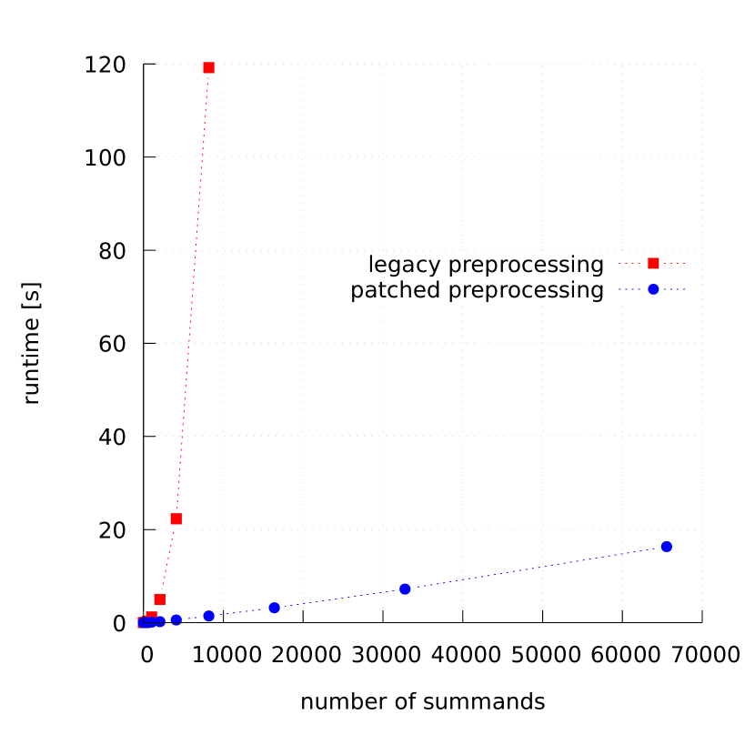
(a) Runtime of preprocessing.

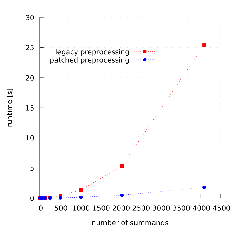
(b) Runtime of solving.

Figure 7: Benchmarks for $\mathsf{sum}_{n}$. The timeout was set to 300 sec and the memory limit was 16GB.

During our experiments we observed that iSAT spends a lot of time in the formula preprocessing steps —  in particular for models involving summations over many terms as they naturally occur in vector and matrix operations. To this end, we used a simple scalable benchmark $\mathsf{sum}_{n}$ asking for a satisfying solution of the equality $y=\sum_{i=0}^{n}\tfrac{1}{n}x_{i}$ with $y,x_{i}\in[0,1]$ for $i=0,\dots,n$ to measure the runtime of iSAT’s preprocessing. We observed an exponential relationship between the problem size $n$ and the runtime of the preprocessing, see the plot ’legacy preprocessing’ in 7(a).

In a deeper analysis, we found that iSAT tends to build an unbalanced abstract syntax tree during parsing and normalisation steps. Hence, recursions over the syntax tree often suffers from the unnecessary depth of the syntax tree. We patched the preprocessing steps of iSAT so that iSAT now builds well-balanced summation terms of minimal depth. Interestingly, this approach also helped to reduce the solving time of iSAT as depicted in 7(b). Both plots in 7(b) still behave exponentially. However, it is noticeable that the plot for the patched version is much flatter compared to the legacy version. Note that in both versions the benchmarks for $n>4096$ yield a memout and, hence, are not depicted in the plots.

A deeper examination of the reasons why also the solving time profits from well-balanced trees and whether these benefits can be extended to other operators is considered as an interesting future work.

3.5 Towards Verification of Safety Properties

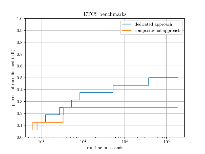
(a) Benchmark results for the dedicated and the composed propagator on the more severe verification ETCS verification task from Sec. 3.2.1.

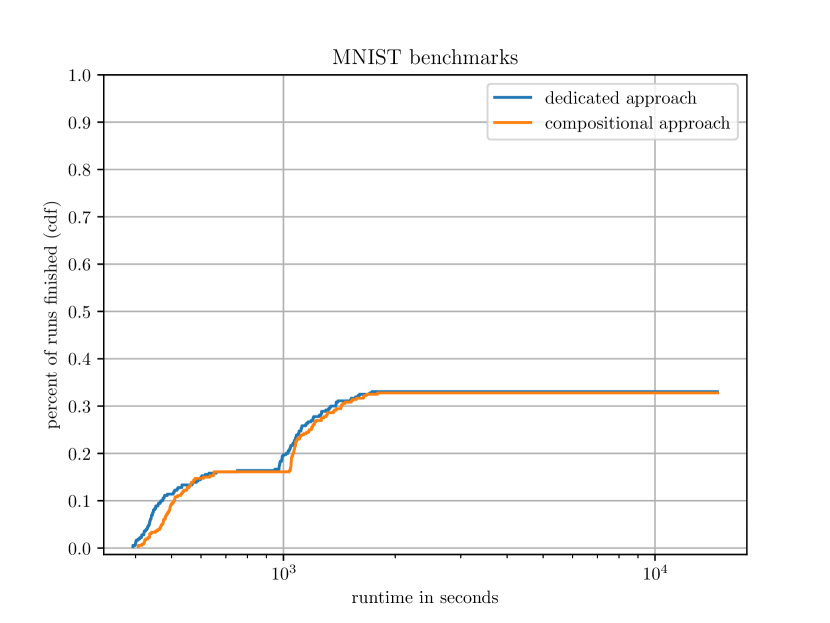
(b) Benchmark results for the dedicated propagator on on the MNIST verification tasks described in Sec. 3.2.2.
nasty fix for caption height

Figure 8: Benchmark results on the somewhat more severe verification tasks. The plots show the proportion of constraint systems that have been solved over time (cumulative distribution function). The benchmarks were performed with the patched iSAT version with a timeout of 4 hours (14,400 seconds).

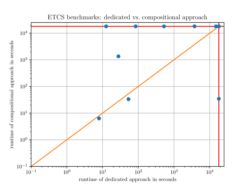
(a) ETCS benchmark

(b) MNIST benchmark

Figure 9: Comparison of the runtimes of the dedicated and the compositional approach on (a) the more severe verification task on the ETCS networks described in Sec. 3.2.1 and (b) the verification task on digit recognition networks described in Sec. 3.2.2. The horizontal axes show the runtimes of the dedicated approach while the vertical axes show the runtimes of the compositional approach (all axes are in logscale). Each data point illustrates the runtimes of the compared approaches on a particular network. Timeouts are located on the red borders. The orange line indicates the line of equal runtime. The benchmarks were performed with the patched iSAT version with a timeout of 4 hours (14,400 seconds).

According to our previous results, in the following we pursued only the compositional and the dedicated approach. Here, we performed benchmarks that were less broadly based but examined somewhat more severe verification tasks, as a successful verification of a safety property corresponds to unsatisfiability result for the negation of the property under investigation. Hence, iSAT has to exclude the presence of (candidate) solutions which is — in general — a more demanding task.

We employed two different benchmark settings to this end, firstly the last ETCS setting from Sec. 3.2.1 in which we try to verify that a network always gives an advisory $\mathit{braking}\equiv\mathrm{true}$ whenever the safety distance is trivially violated, and secondly the MNIST scenario where we try to prove the absence of adversarial images within some small $\varepsilon$-box around images we sampled from the MNIST database as described in Sec. 3.2.2.

The result for the ETCS setting are illustrated in 8(a). The figure shows cumulative distribution functions, i.e. the proportion of terminated solver runs plotted over the runtime. Here, we can clearly identify that the dedicated approach can solve more constraint systems ($8$ out of $16$, i.e. $50\%$) within the time limit than the compositional approach ($25\%$). The compositional approach was able to prove two networks to be safe, i.e. iSAT terminated with “unsatisfiable” for the networks with $12$ nodes per layer and $2$ and $5$ layers respectively. These networks were also proven to be safe by the dedicated approach, plus $4$ additional networks ($2$ layers with $50$ and $100$ nodes per layer, $3$ layers with $12$ nodes per layer, and $4$ layers with $50$ nodes per layer) for which the compositional approach was aborted due to timeout.

A somewhat different result is shown for the MNIST benchmark in 8(b): No clear distinction between the two approaches is possible wrt. the cumulative distribution function. We cannot even determine, apart from outliers, that there are constraint systems for which one or the other approach is faster and that these differences balance out in total. 9(b) reveals that — apart from outliers — the runtime is essentially equal for almost all constraint systems. The absolute numbers also do not exhibit significant differences: The dedicated approach was aborted due to timeout in $241$ cases ($66.94\%$ timeout rate) and proved $119$ networks to be safe ($33.06\%$) while the compositional approach was aborted in $242$ cases ($67.22\%$ timeout rate) and proved $118$ networks to be safe ($32.78\%$). Successful verification of the desired property and timeouts were distributed almost equally over both network sizes for both approaches.

We thus cannot clearly conclude from these results of our second evaluation step, that the dedicated approach is always to be preferred over the compositional approach when aiming at severe verification tasks.

4 Conclusion

The aim of our paper was to investigate to what extent iSAT, an SMT solver that inherently supports nonlinear and transcendental functions, is suitable for the automatic verification of severe safety properties of ANNs. To this end, we first considered three different encoding approaches for the functional relation of an ANN. While the layer-wise weighted summation over input neurons can be encoded as linear combinations, these approaches differ in their handling of the sigmoid activation function. In the approximating approach the sigmoid activation function is replaced by encapsulating interval boxes which is inherently inexact. The compositional and the dedicated approach fully rely on iSAT’s ability to handle nonlinear and transcendental functions, whereas the dedicated approach required the implementation of a sigmoid propagator into iSAT explicitly. In our preliminary investigation, we noticed that the preprocessing of iSAT shows some weaknesses with regard to the treatment of extensive linear combinations, which we were able to eliminate by a patch. Thereafter, we could finally turn to the verification of severe safety properties.

Through our investigation, we were able to determine that it is not worthwhile to rely on the approximating approach, neither in terms of runtime nor the quality of the results. It is more advisable to rely on the strengths of iSAT’s nonlinear and transcendental propagators, either following the compositional or the dedicated approach. While our preliminary investigation and also the verification of safety properties for the ETCS example suggest a rather clear preference for the dedicated approach, we could not fully confirm this impression for the verification of safety properties in the MNIST example.

A preliminary conclusion is that the dedicated propagator can be useful, but compared to the compositional approach, one must critically ask oneself whether the implementation effort is justified. We can therefore recommend the implementation of a dedicated propagator only for activation functions that occurs sufficiently often in the networks to be examined.

Another important observation is that the solving time of iSAT strongly depends on the network structure, its size, and the verification targets. Regarding the network structure, a closer look at the internal processes of iSAT seems to be useful, as our experiences with the preprocessing issues already revealed. For example, we could not conclusively clarify what role the increased Boolean complexity of the approximating approach played. Especially with regard to the comparison of the dedicated and compositional approach, a deeper investigation of iSAT’s splitting mechanism and its various heuristics seems to be important. It is not clear whether the additional splitting possibilities on the auxiliary variables that are necessary for the compositional approach are sometimes beneficial. However, during our experiments, we tried different splitting heuristics without getting a clear prioritisation of one of these heuristics.

Despite all these imponderables, we have nevertheless seen that iSAT is able to verify networks with nontrivial nonlinear activation functions. We see the strength of iSAT here not so much in the treatment of the linear components, but rather in the ability to quickly support a large variety of nonlinear activation functions through a compositional approach, as well as in the possibility to extend iSAT by dedicated propagators when a performance improvement is expected due to such an extension.

As future work, we plan to further investigate the relationship of the network structure and the verification targets with iSAT’s internal processes with the aim to identify those settings where implementing a dedicated propagator pays off. On the other hand, our results also suggest to extend our translation toolchain to the point where a wide variety of activation functions is supported by the compositional approach fully automatically. Looking at the rapidly growing number of verification tools, a comparison of runtime and precision of verdicts with other tools is also indispensable.

References

- [1]
- [2] ETH Robustness Analyzer for Neural Networks (ERAN) github repository. https://github.com/eth-sri/eran, last accessed 2021-04-10.
- [3] François Chollet: Keras. https://keras.io/, last accessed 2021-02-19.
- [4] Martin Davis, George Logemann & Donald Loveland (1962): A Machine Program for Theorem-Proving. Communications of the ACM 5(7), p. 394–397, 10.1145/368273.368557.
- [5] Martin Fränzle, Christian Herde, Stefan Ratschan, Tobias Schubert & Tino Teige (2007): Efficient solving of large non-linear arithmetic constraint systems with complex boolean structure. Journal of Satisfiability, Boolean Modeling and Computation, pp. 209–236, 10.3233/SAT190012.
- [6] Braddock Gaskill (2018): ONNX: the Open Neural Network Exchange Format. Linux Journal. Available at https://www.linuxjournal.com/content/onnx-open-neural-network-exchange-format. Last accessed 2021-10-27.
- [7] Timon Gehr, Matthew Mirman, Dana Drachsler-Cohen, Petar Tsankov, Swarat Chaudhuri & Martin Vechev (2018): AI2: Safety and Robustness Certification of Neural Networks with Abstract Interpretation. In: 2018 IEEE Symposium on Security and Privacy (SP), pp. 3–18, 10.1109/SP.2018.00058.
- [8] Christian Herde (2011): Efficient Solving of Large Arithmetic Constraint Systems with Complex Boolean Structure: Integration of DPLL and Interval Constraint Solving - ETCS model. Vieweg+Teubner Research, 10.1007/978-3-8348-9949-1.
- [9] Xiaowei Huang, Marta Kwiatkowska, Sen Wang & Min Wu (2017): Safety Verification of Deep Neural Networks. In Rupak Majumdar & Viktor Kunčak, editors: Computer Aided Verification, Springer, pp. 3–29, 10.1007/978-3-319-63387-9_1.
- [10] Radoslav Ivanov, James Weimer, Rajeev Alur, George J. Pappas & Insup Lee (2019): Verisig: Verifying Safety Properties of Hybrid Systems with Neural Network Controllers. In: Proceedings of the 22nd ACM International Conference on Hybrid Systems: Computation and Control, HSCC ’19, Association for Computing Machinery, New York, NY, USA, p. 169–178, 10.1145/3302504.3311806.
- [11] Guy Katz, Clark W. Barrett, David L. Dill, Kyle Julian & Mykel J. Kochenderfer (2017): Reluplex: An Efficient SMT Solver for Verifying Deep Neural Networks. In Rupak Majumdar & Viktor Kunčak, editors: Computer Aided Verification, Springer, pp. 97–117, 10.1007/978-3-319-63387-9_5.
- [12] Guy Katz, Derek A. Huang, Duligur Ibeling, Kyle Julian, Christopher Lazarus, Rachel Lim, Parth Shah, Shantanu Thakoor, Haoze Wu, Aleksandar Zeljić, David L. Dill, Mykel J. Kochenderfer & Clark Barrett (2019): The Marabou Framework for Verification and Analysis of Deep Neural Networks. In Isil Dillig & Serdar Tasiran, editors: Computer Aided Verification, Springer International Publishing, Cham, pp. 443–452, 10.1007/978-3-030-25540-4_26.
- [13] Diederik P. Kingma & Jimmy Ba (2017): Adam: A Method for Stochastic Optimization. Available at https://arxiv.org/abs/1412.6980.
- [14] Alex Krizhevsky (2009): Learning multiple layers of features from tiny images. Technical Report, Department of Computer Science, University of Toronto. Available at https://www.cs.toronto.edu/~kriz/cifar.html.
- [15] Alex Krizhevsky, Ilya Sutskever & Geoffrey Hinton (2012): ImageNet Classification with Deep Convolutional Neural Networks. Neural Information Processing Systems 25, 10.1145/3065386.
- [16] Yann LeCun, Corinna Cortes & Christopher J. C. Burges: MNIST. http://yann.lecun.com/exdb/mnist/, last accessed 2021-07-08.
- [17] Guido Manfredi & Yannick Jestin (2016): An introduction to ACAS Xu and the challenges ahead. In: 2016 IEEE/AIAA 35th Digital Avionics Systems Conference (DASC), pp. 1–9, 10.1109/DASC.2016.7778055.
- [18] Leonardo de Moura & Nikolaj Bjørner (2008): Z3: An Efficient SMT Solver. In C. R. Ramakrishnan & Jakob Rehof, editors: Tools and Algorithms for the Construction and Analysis of Systems, Springer, pp. 337–340, 10.1007/978-3-540-78800-3_24.
- [19] Luca Pulina & Armando Tacchella (2010): An Abstraction-Refinement Approach to Verification of Artificial Neural Networks. In Tayssir Touili, Byron Cook & Paul Jackson, editors: Computer Aided Verification, Springer, pp. 243–257, 10.1007/978-3-642-14295-6_24.
- [20] Luca Pulina & Armando Tacchella (2012): Challenging SMT Solvers to Verify Neural Networks. AI Commun. 25(2), pp. 117–135, 10.3233/AIC-2012-0525. Available at http://dl.acm.org/citation.cfm?id=2350156.2350160.
- [21] Francesca Rossi, Peter van Beek & Toby Walsh (2006): Handbook of Constraint Programming (Foundations of Artificial Intelligence). Elsevier Science Inc., USA.
- [22] Karsten Scheibler, Leonore Winterer, Ralf Wimmer & Bernd Becker (2015): Towards Verification of Artificial Neural Networks. In Ulrich Heinkel, Daniel Kriesten & Marko Rößler, editors: Methoden und Beschreibungssprachen zur Modellierung und Verifikation von Schaltungen und Systemen, Technische Universität Chemnitz Professur Schaltkreis- und Systementwurf, pp. 30–40.
- [23] Siddharth Sharma, Simone Sharma & Anidhya Athaiya (2020): Activation Functions in Neural Networks. International Journal of Engineering Applied Sciences and Technology 4, pp. 310–316, 10.33564/IJEAST.2020.v04i12.054.
- [24] Weiming Xiang, Patrick Musau, Ayana A. Wild, Diego Manzanas Lopez, Nathaniel Hamilton, Xiaodong Yang, Joel Rosenfeld & Taylor T. Johnson (2018): Verification for Machine Learning, Autonomy, and Neural Networks Survey. Available at https://arxiv.org/pdf/1810.01989.pdf.