AB Aur, a Rosetta stone for studies of planet formation (II): $\rm H_{2}S$ detection and sulfur budget

Abstract

Context. The sulfur abundance is poorly known in most environments. Yet, deriving the sulfur abundance is key to understanding the evolution of the chemistry from molecular clouds to planetary atmospheres. We present observations of $\rm H_{2}S$ $\rm 1_{10}-1_{01}$ at 168.763 GHz toward the Herbig Ae star AB Aur.

Aims. We aim to study the abundance of sulfuretted species toward AB Aur and to constrain how different species and phases contribute to the sulfur budget.

Methods. We present new NOrthern Extended Millimeter Array (NOEMA) interferometric observations of the continuum and $\rm H_{2}S$ $\rm 1_{10}-1_{01}$ line at 168.763 GHz toward AB Aur. We derived radial and azimuthal profiles and used them to compare the geometrical distribution of different species in the disk. Assuming local thermodynamical equilibrium (LTE), we derived column density and abundance maps for H₂S, and we further used Nautilus to produce a more detailed model of the chemical abundances at different heights over the mid-plane at a distance of r=200 au.

Results. We have resolved H₂S emission in the AB Aur protoplanetary disk. The emission comes from a ring extending from 0.67$\arcsec$ ($\rm\sim$109 au) to 1.69$\arcsec$ ($\rm\sim$275 au). Assuming T=30 K, n_H=10$\rm{}^{9}\leavevmode\nobreak\ cm^{-3}$, and an ortho-to-para ratio of three, we derived a column density of (2.3$\rm\pm$0.5)$\rm\times 10^{13}\leavevmode\nobreak\ cm^{-2}$. Under simple assumptions, we derived an abundance of (3.1$\rm\pm$0.8)$\rm\times 10^{-10}$ with respect to H nuclei, which we compare with Nautilus models to deepen our understanding of the sulfur chemistry in protoplanetary disks. Chemical models indicate that H₂S is an important sulfur carrier in the solid and gas phase. We also find an important transition at a height of $\rm\sim$12 au, where the sulfur budget moves from being dominated by ice species to being dominated by gas species.

Conclusions. We confirm that present-day models still struggle to simultaneously reproduce the observed column densities of the different sulfuretted species, and the observed abundances are still orders of magnitude away from the cosmic sulfur abundance. Studying sulfuretted species in detail in the different phases of theinterstellar medium is key to solving the issue.

1 Introduction

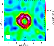
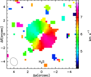
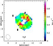
Figure 1: From left to right, zeroth-, first-, and second-moment maps of the H₂S 1₁₀-1₀₁ emission line toward AB Aur. The synthesized beam is shown in the lower left corner of each plot.

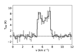
Figure 2: Stacked $\rm H_{2}S$ 1$\rm{}_{01}-1_{10}$spectrum of AB Aur inside the 5$\rm\sigma$ emission contour levels. The gray spectrum depicts the observed spectrum, and the black one depicts the same after rebinning.

Protoplanetary disks are the birthplace of planets, implying that a planet’s composition is, at least partially, inherited from the disk. The protoplanetary disk chemical composition, in turn, is inherited from the natal molecular cloud, but modified by the prevailing physical conditions of protoplanetary disks. To study the chemical complexity of planetary atmospheres, one must understand that of protoplanetary disks. A topic of major interest due to its possible implications for the emergence of life is the chemical evolution of molecules that carry the six key elements in organic chemistry: H, C, O, N, S, and P.

Sulfur is the tenth most abundant element in the Universe and plays a crucial role in biological systems. The abundance toward the Sun (Asplund et al. 2009, S/H$\sim$1.5$\times$10^-5) agrees well with the value derived toward Orion B stars for example (S/H$\sim$1.4$\times$10^-5, Daflon et al. 2009). However, its chemistry is poorly understood in interstellar environments, and sulfuretted molecules are not as abundant as expected in the interstellar medium (ISM). While sulfur abundance is close to the cosmic value in the diffuse ISM and photon-dominated regions (PDRs) (Goicoechea et al. 2006; Howk et al. 2006; Goicoechea & Cuadrado 2021), it is strongly depleted in the dense molecular gas ($\rm>$10$\rm{}^{4}\leavevmode\nobreak\ cm^{-3}$), where only 0.1% of the sulfur cosmic abundance is observed (Tieftrunk et al. 1994; Wakelam et al. 2004; Vastel et al. 2018). A study of the sulfur content in dense cores by Hily-Blant et al. (2022) provides evidence for a progressive depletion of sulfur with age, as well as with density for a given core. It is expected that most of the sulfur is then locked on the icy mantles of dust grains in dense cores (Millar & Herbst 1990; Ruffle et al. 1999; Vidal et al. 2017; Laas & Caselli 2019). However, only solid OCS has been unambiguously detected on the ice mantles of these objects thanks to the strength of its infrared band (Geballe et al. 1985; Palumbo et al. 1995). Furthermore, SO₂ has also been tentatively detected (Boogert et al. 1997). Since only upper limits for the solid H₂S abundance could be derived thus far (Jiménez-Escobar & Muñoz Caro 2011) and since detection is hampered by the strong overlap between the 2558 cm^-1 band and the methanol bands at 2530 and 2610 cm^-1, the main gas and solid phase sulfur reservoirs thus remain unknown.

Sulfur-bearing species have been widely detected in the Solar System. In comets, they are detected mostly in the form of H₂S and S₂ (Mumma & Charnley 2011). Hale Bopp showed a large variety of detections, including CS and SO (Boissier et al. 2007). Furthermore, CS was also detected toward the comets C/2012 F6 (Lemmon) and C/2014 Q2 (Lovejoy) (Biver et al. 2016). Using the Rosetta Orbiter Spectrometer for Ion and Neutral Analysis (ROSINA (Balsiger et al. 2007)) on board Rosetta, H₂S, S, SO₂, SO, OCS, H₂CS, CS₂, and S₂ were detected in the coma (Le Roy et al. 2015) of 67P/Churyumov-Gerasimenko. In addition, S₃, S₄, CH₃SH, and C₂H₆S were also detected (Calmonte et al. 2016). Considering the variety of S species detected, the mean abundance of H₂S relative to H2O remains around 1.5% (Bockelée-Morvan & Biver 2017) with values ranging from $\rm 10^{-3}$ to 0.1.

Protoplanetary disks (PPDs) are expected to strongly affect the abundance of different sulfuretted species given the multiple chemical reprocessing mechanisms at work in them. Therefore, they are key to understanding the huge differences (at a factor of a thousand) in the sulfur abundances between the diffuse ISM and dense molecular gas. Searches for S-bearing molecules in PPDs have provided few detections. Thus far, only one S species, CS, has been widely detected (Dutrey et al. 2011; Guilloteau et al. 2012; Pacheco-Vázquez et al. 2015; Guilloteau et al. 2016; Podio et al. 2020a, b; Rosotti et al. 2021; Rivière-Marichalar et al. 2021; Nomura et al. 2021). We note that H₂CS was detected in MWC 480 (Le Gal et al. 2019), and H₂S was detected in GG Tau (Phuong et al. 2018) and in four protoplanetary disks in Taurus (Rivière-Marichalar et al. 2021). Furthermore, SO has been detected in a few PPDs (Pacheco-Vázquez et al. 2016; Booth et al. 2018, 2021; Le Gal et al. 2021), and SO₂ has been observed toward IRS 48 as well (Booth et al. 2021). Recently, CCS was detected toward GG Tau (Phuong et al. 2021), but the low signal-to-noise ratio (s/n) precluded the analysis of the spatial distribution. The authors could not reproduce the observed CCS column density together with other sulfuretted species, supporting the idea that astrochemical sulfur networks are incomplete. Similar problems have been encountered in CS studies, such as in the study of cold cores by Navarro-Almaida et al. (2020), where models overpredicted CS abundances by a factor of 10. Sulfur astrochemical networks have improved over the last years (Fuente et al. 2016, 2017b; Le Gal et al. 2017; Vidal et al. 2017; Fuente et al. 2019; Laas & Caselli 2019), including new formation and destruction routes, but work is still needed to solve the issue.

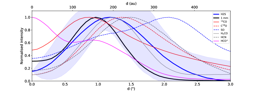
Figure 3: H₂S azimuthally averaged radial profile compared to previous observations by this team. All the intensity maps have been convolved to match the beam size of our H₂S emission line maps. The light-blue shaded area depicts the H2S radial profile plus or minus uncertainties.

The Herbig star AB Aur is a well-known Herbig A0-A1 (Hernández et al. 2004) star that hosts a transitional disk. The system is located at 162.9 pc from the Sun (Gaia Collaboration 2018), and it is perfectly suited to study the spatial distribution of gas and dust in circumstellar environments in detail. The disk extends out to a radius of 2.3$\arcsec$ ($\rm\sim$373 au) in the continuum (Rivière-Marichalar et al. 2020). Molecular emission from species such as CS, C¹⁸O, SO, H2CO, and H2S is observed with radii of emission peaks ranging from 0.9$\arcsec$ to 1.4$\arcsec$. The disk depicts a series of features that could be linked to planet formation, such as prominent spiral arms at the near-IR and radio wavelengths. The system also presents a cavity in continuum emission (Piétu et al. 2005; Tang et al. 2012; Fuente et al. 2017a) that extends to $\sim$70-100 au. Tang et al. (2012) discovered a compact source inside the cavity, which is most likely an inner disk well suited to explain the strong accretion observed toward the source (Garcia Lopez et al. 2006; Salyk et al. 2013). Rodríguez et al. (2014) detected a radio jet consistent with the high levels of accretion observed. Inside the dust cavity, prominent CO spiral arms were observed by Tang et al. (2017) using the Atacama Large Millimeter/submillimeter Array (ALMA). Other species have been detected toward AB Aur by different studies, including CO, SO, HCO+, HCN, and H2CO (Schreyer et al. 2008; Piétu et al. 2005; Tang et al. 2012, 2017; Fuente et al. 2010; Pacheco-Vázquez et al. 2015, 2016; Rivière-Marichalar et al. 2019a; Rivière-Marichalar et al. 2020). The first detection of SO in a protoplanetary disk was reported, in fact, also toward AB Aur (Fuente et al. 2010; Pacheco-Vázquez et al. 2015, 2016). In Rivière-Marichalar et al. (2019a), we presented high angular resolution the NOrthern Extended Millimeter Array (NOEMA) observations of HCN and HCO+, with a beam size of 0.4$\arcsec$. The HCO+ map depicts an outer disk with decay in intensity coincident with the dust cavity, a compact source toward the center, and a bridge of material that connects the outer disk with the compact source in the center. In paper I of this series, we presented the results of a NOEMA spectral survey in AB Aur (Paper I, Rivière-Marichalar et al. 2020), where we were able to obtain zeroth-, first-, and second-moment maps, opacity maps, temperature maps, and column density maps of the transitions and species surveyed. These species included $\rm{}^{12}CO$, $\rm{}^{13}CO$, C$\rm{}^{18}O$, H2CO, and SO. We derived a mean disk temperature of 39 K, and column densities in the range 10¹² to 5$\times$10$\rm{}^{13}\leavevmode\nobreak\ cm^{-2}$ for H₂CO, SO, HCO⁺ and HCN, and $\rm\sim 10^{17}\leavevmode\nobreak\ cm^{-2}$ for $\rm{}^{13}CO$. We computed a gas-to-dust mass ratio map of AB Aur and showed it to range from 10 to 40 across the disk, with larger values close to the disk’s inner edge. Such values are between two times and one order of magnitude smaller than the typical value of 100 found in the ISM. The minimum in the gas-to-dust mass ratio was coincident with the peak of the continuum emission, indicating a particularly gas-poor dust trap. We produced radially and azimuthally averaged profiles of line intensity, temperature, and column densities. Such profiles demonstrate the strong chemical segregation observed in the source, with differences as high as 100 au in the position of their peaks.

In this paper, we present the first detection of H2S toward AB Aur obtained with NOEMA. In Sect. 2 we introduce the observations setup and summarize the reduction process. In Sect. 3 we present our results, including estimates of the H2S column density and abundance. In Sect. 5 we discuss the implications of our results for the topic of sulfur chemistry in protoplanetary disks. Finally, in Sect. 6 we summarize our conclusions.

2 Observations and data reduction

We observed the H₂S 1₁₀-1₀₁ transition at 168.763 GHz toward AB Aur with NOEMA between May and July 2020 using EMIR receivers (Carter et al. 2012). The source was observed for eight hours in configuration 8, with baselines ranging from 18 to 315 m. The data reduction and map synthesis was performed using GILDAS/MAPPING. We used the PolyFix correlator centered at 161.5 GHz with a bandwidth of 8 GHz per sideband. A chunk with a spectral resolution of 62.5 kHz was placed at 168.763 GHz to observe H₂S 1₁₀-1₀₁, reaching a velocity resolution of 0.1 km s^-1. The final map was built using robust weight, allowing us to reach a beam size of 1.19$\arcsec\times$0.97$\arcsec$ (193 au $\rm\times$ 158 au), with PA=34^∘ the PA defined as positive from N to E.

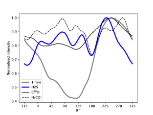
Figure 4: H₂S azimuthal cuts compared to previous observations by this team. All the intensity maps have been convolved to match the beam size of our H₂S emission line maps. The azimuthal profiles shown were computed at the distance of the emission peak of each species. The profiles were normalized with respect to their respective peaks.

3 Results

We show in Fig. 1 the resulting zeroth-, first- and second-moment maps of H₂S 1₁₀-1₀₁ at 168.763 GHz. The integrated intensity map depicts a ring of H₂S emission extending from $\rm\sim$0.7$\arcsec$ ($\rm\sim$114 au) to $\rm\sim$1.7$\arcsec$ ($\rm\sim$277 au). The ring shows strong azimuthal asymmetries, with a peak that is roughly coincident with the position of the continuum peak (Fuente et al. 2017a) and the position of the H₂CO (Rivière-Marichalar et al. 2020) and HCN (Rivière-Marichalar et al. 2019a) integrated emission peaks.

In Fig. 2 we show the stacked spectrum inside the 5$\sigma$ emitting contours. The spectrum depicts the two-peaked profile characteristic of a rotating disk. The two peaks show similar intensities (8.3 K and 8.8 K), and line widths (0.4 and 0.54 km s^-1). The blue-shifted component peaks at 5.4 km s^-1, and the red-shifted one at 7.0 km s^-1.

In Fig. 3 we show the azimuthally averaged radial profile of the H₂S 1₁₀-1₀₁ emission line and compare it to the radial profile of other transitions that have been observed with high spatial resolution toward AB Aur, including ¹²CO, ¹³CO, C¹⁸O, SO, and H₂CO (Rivière-Marichalar et al. 2020), and HCO⁺ and HCN (Rivière-Marichalar et al. 2019a). These maps have been deprojected, assuming an inclination angle i = 26^∘ and position angle PA = -37^∘. The maps were also convolved with the H₂S beam for a better comparison of the radial profiles. The H2S emission ring shows a peak at $\rm\sim$1.2$\arcsec$ ($\rm\sim$195 au), with emission in excess over the RMS extending from $\rm\sim$0.51$\rm\arcsec$ ($\rm\sim$83 au) to $\rm\sim$2.35$\rm\arcsec$ ($\rm\sim$383 au). The average disk width is 1.84$\rm\arcsec$ ($\rm\sim$300 au). H2S shows a radial profile that matches that of H2CO. In a recent study of H2S emission in Taurus disks, a tentative correlation between H2S and H2CO was shown (Rivière-Marichalar et al. 2021); our maps now point to a very similar spatial origin for both emission lines, increasing the observational support for such a correlation. Furthermore, both species have formation routes on the surface of grains. In Fig. 4 we show cuts in azimuth of the H2S, H2CO, C¹⁸O, and continuum emission maps at the radius of their respective emission peaks. The similarity between H2S and H2CO is again prominent, with local maxima and minima at almost the same azimuths. The azimuthal contrast ratio of H2S at the distance to the emission peak is 1.5 $\rm\pm$ 0.3.

Assuming local thermodynamical equilibrium (LTE) we compute an H2S column density map. Since we have observed only one o-H2S transition ($\rm 1_{10}-1_{01}$) no rotational diagram could be computed and we thus assumed a fixed disk temperature. For consistency, we adopted a temperature of 30 K as in our previous work (Rivière-Marichalar et al. 2020), allowing the comparison between H2S and the species surveyed in this work. The mean o-H2S column density is (1.5$\rm\pm$0.3)$\rm\times 10^{13}\leavevmode\nobreak\ cm^{-2}$, with a minimum value of 1.0$\rm\times 10^{13}\leavevmode\nobreak\ cm^{-2}$ and a maximum of 2.2$\rm\times 10^{13}\leavevmode\nobreak\ cm^{-2}$. Assuming that H2S behaves like H2O, we assign an ortho-to-para ratio of 3 (Hama et al. 2016), and derive a H2S mean column density of (1.9$\rm\pm$0.4)$\rm\times 10^{13}\leavevmode\nobreak\ cm^{-2}$. The resulting deconvolved column density map is shown in Fig. 5. The peak in column density is coincident with the dust trap. There are other two local maxima at PA$\rm\sim 90^{\circ}$ and $\rm\sim 135^{\circ}$.

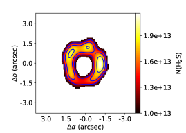
Figure 5: H2S column density map computed assuming LTE and T_k = 30 K and ortho-to-para ratio of 3. The map has been deprojected assuming an inclination angle i = 26^∘ and position angle PA = -37^∘.

4 Modeling the sulfur budget in AB Aur

To gain further insight into the AB Aur sulfur budget, we also computed a Nautilus 1D model. Nautilus computes the evolution of molecular abundances for a set of initial abundances and physical parameters using gas-phase, gas-grain, and surface chemistry reactions (Semenov et al. 2010; Loison et al. 2014; Wakelam et al. 2014; Reboussin et al. 2015). The parameters include gas and dust temperature, gas density, cosmic ray molecular hydrogen ionization rate $\rm\zeta_{H_{2}}$, and extinction, among others. A refinement of the code considers grain surface and grain mantle reactions by using a three-phase structure that includes gas, grain surfaces, and grain mantles (Ruaud et al. 2016; Wakelam et al. 2017). For a more detailed description of the code see Ruaud et al. (2016) and Wakelam et al. (2017).

Table 1: Nautilus model input parameters for the molecular cloud prephase and the protoplanetary disk at r=200 au.

Parameter	Value
Molecular cloud
$\rm T_{gas}$ (K)	10
$\rm T_{dust}$ (K)	10
nH	104
$\rm A_{v}$	20
fUV (Draine units)	1
$\rm\zeta_{H_{2}}$ (s-1)	$\rm 10^{-17}$
Gas-to-dust mass ratio	100
AB Aur at r=200 au
$\rm T_{mid}$ (K)	39
$\rm T_{atm}$ (K)	65
$\rm A_{v}$	2
f$\rm{}_{UV}(Draineunits)$	1.2$\rm\times 10^{4}$
$\rm\zeta_{H_{2}}$ (s-1)	$\rm 10^{-17}$
Gas-to-dust mass ratio	40

Table 2: Initial abundances

Species	$n_{i}/n_{\text{H}}$	Reference
H2	0.5	-
He	9.0$\times$10-2	1
C+	1.7$\times$10-4	2
N	6.2$\times$10-5	2
O	2.4$\times$10-4	3
S+	1.5$\times$10-5	4
Si+	8.0$\times$10-9	4
Fe+	3.0$\times$10-9	4
Na+	2.0$\times$10-9	4
Mg+	7.0$\times$10-9	4
P+	2.0$\times$10-10	4
Cl+	1.0$\times$10-9	4
F+	6.7$\times$10-9	5

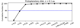
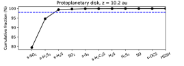
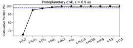
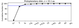
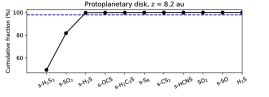
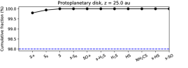
Figure 6: Cumulative abundance fraction of sulfuretted species from Nautilus models at different heights above the midplane at r=200 au. The horizontal blue dashed line depicts the position of the 98% cumulative fraction.

4.1 Model setup

The physical structure used in our models is the one used in Rivière-Marichalar et al. (2020), which in turn was adapted from Le Gal et al. (2019). Given the moderate resolution of the observations, we decided not to consider the radial structure and instead focus on the vertical profile at a radius of r=200 au, representative of the H2S ring described in Sect. 2. Our models included both photodesorption (with a yield of 10^-4molecules photon^-1) and chemical desorption, assuming the conditions listed in Table 1. Chemical desorption was included following the prescription by Garrod et al. (2007) for ice-coated grains implemented in Nautilus. To mimic the molecular cloud origin of the system, instead of assuming initial abundances following cosmic values, we computed a 10 K molecular cloud model and used its output abundances as the initial abundances for our 1D protoplanetary disk model. Each phase was let to evolve for 1 Myr. The input physical parameters for this model are listed in Table 1, and the initial abundances used for the molecular cloud prephase are listed in Table 2. We note that we use a nondepleted value for the sulfur abundance. Nautilus assumes a single size of 0.1 $\rm\mu$m for the dust grains. Following Rivière-Marichalar et al. (2020), we assumed a gas-to-dust mass ratio of 40 for the AB Aur protoplanetary disk. The chemical network used is the updated version of the kida.uva.2014 (Wakelam et al. 2015) presented in Navarro-Almaida et al. (2020) which includes an enhanced chemical network for sulfur chemistry (Vidal et al. 2017). The grid consisted of 100 heights over the mid-plane with logarithmic spacing. We note that Nautilus is not properly suited to model the PDR-like conditions of the uppermost layers of the disk model. Diffusion between neighboring cells was not included. Since the distinction between mantle species and surface species is mostly a computational parametrization in Nautilus, in the following we consider grain surfaces and mantles as a single phase, called grain surface and preceded by the prefix g-, which is computed by adding up abundances in each of the solid phases (mantle and surface of grains) for each species.

For the sake of clarity, we summarize in the following the main equations describing our model. The vertical temperature profile at r=200 au follows the prescription by Dartois et al. (2003) used in Rosenfeld et al. (2013), described by the following equation:

$$\small T(z)=\left\{\begin{array}[]{ll}T_{\rm{mid}}+(T_{\rm{atm}}-T_{\rm{mid}})\left[\sin\left(\frac{\pi z}{2z_{q}}\right)\right]^{2\delta}&\mbox{if}\,z<z_{q}\\ T_{\rm{atm}}&\mbox{if}\,z\geq z_{q},\end{array}\right.$$ (1)

where $\rm T_{atm}$ and $\rm T_{mid}$ are the temperature of the disk atmosphere and the disk mid plane at r= 200 au, respectively.

$$T_{\rm{mid}}=T_{\mathrm{mid},R_{c}}\,\left(\frac{{\rm 200\leavevmode\nobreak\ au}}{R_{\rm{c}}}\right)^{-q},$$ (2)

$$T_{\rm{atm}}=T_{\mathrm{atm},R_{c}}\,\left(\frac{{\rm 200\leavevmode\nobreak\ au}}{R_{\rm{c}}}\right)^{-q},$$ (3)

where $R_{c}$ is a characteristic radius ($R_{c}$=98 au, Rivière-Marichalar et al. 2020), and $z_{q}=4H$, where H is the pressure scale height.

$$H=\sqrt{\frac{k_{\rm B}\,T_{\rm mid}\,r^{3}}{\mu\,m_{\rm H}\,G\,M_{\star}}},$$ (4)

where $k_{\rm{B}}$ is the Boltzmann constant, $\mu=2.4$ is the mean molecular weight of the gas, $m_{\rm{H}}$ is the proton mass, and $M_{\star}$ is the mass of the central star. The mid-plane temperature $T_{\rm mid}$ is described by equation

$$T_{\rm{mid}}(r)\approx\left(\frac{\varphi L_{\star}}{8\pi r^{2}\sigma_{\rm{SB}}}\right)^{1/4},$$ (5)

where $L_{\star}$ is the stellar luminosity, $\varphi$ is the flaring index, and $\sigma_{\rm{SB}}$ is the Stefan-Boltzman constant. We assumed that the dust has the same temperature as the gas. The vertical profile of the density is described by

$$\rho(z)=\rho_{0}e^{-\frac{z^{2}}{2H^{2}}},$$ (6)

where $\rho_{0}$ is the mid-plane density of the gas at 200 au. Finally, the UV flux at a given radius is given by equation

$$f_{\rm{UV}}=\frac{0.5f_{\rm{UV},R_{c}}}{\left(\frac{r}{R_{c}}\right)^{2}+\left(\frac{4\rm{H}}{R_{c}}\right)^{2}}.$$ (7)

Table 3: List of species that contain 98% of the sulfur budget at r=200 au in our Nautilus model.

Species	Abundance	Fraction of total (%)
Molecular cloud
S	3.9$\rm\times 10^{-6}$	26.0
g-HS	3.8$\rm\times 10^{-6}$	25.4
g-H2S	3.3$\rm\times 10^{-6}$	22.2
g-NS	2.7$\rm\times 10^{-6}$	17.8
g-S	5.9$\rm\times 10^{-7}$	3.9
g-OCS	1.9$\rm\times 10^{-7}$	1.2
CS	1.7$\rm\times 10^{-7}$	1.1
AB Aur
g-H2S	9.2$\rm 10^{-6}$	61.4
g-SO2	2.6$\rm\times 10^{-6}$	17.3
g-H2S3	4.6$\rm\times 10^{-7}$	9.2
S+	1.0$\rm\times 10^{-6}$	6.9
g-CS2	1.2$\rm\times 10^{-7}$	1.6
S	1.9$\rm\times 10^{-7}$	1.3

4.2 Model results

In Fig. 6, we show the cumulative fraction of the total sulfur abundance for the ten most abundant sulfuretted species computed by Nautilus at different heights for a given radius of 200 au, where the pressure scale height H is $\rm\sim$ 8 au. The prefix s means that the species are on the surface of dust grains. The lack of prefix means that the species are in gaseous form. The obtained distribution does not change much from z=0.1 au ($\rm A_{v}\sim$29 mag) to z$\rm<$7 au ($\rm A_{v}\sim$11.5 mag). At these heights, most of the sulfur is in the form of H₂S on the surface of grains (more than 95% of the cosmic abundance at z=0.1 au, and 65% at z$\rm\sim$7 au). At z$\rm\sim$8 au H2S3 and SO2 in the surface of grains become the dominant carriers. At z=10, the budget is dominated by SO2 on the surface of grains (79% of the cosmic sulfur abundance). At z=15 au, the budget becomes dominated by two gas species: S⁺ and S contain 97% of the sulfur abundance. Finally, at z=25 au, 99.8% is in the form of S⁺.

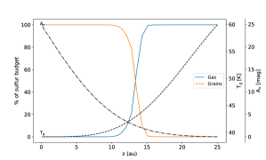
Figure 7: Percentage of the sulfur abundance contained in the different phases of the model as a function of height at 200 au: in the mantle of grains, in the surface of grains, and in gas phase.

The trends with the height of the different phases of the model are summarized in Fig. 7, where we represent the percentage of the sulfur cosmic abundance contained in each of the phases that are considered by the model (sulfur species in the surface of dust grains and gas-phase species) as a function of the height over the mid-plane at r=200 au. As can be seen, before $\rm\sim$14 au the budget is dominated by surface species. Then, around 12 au, chemical species in the gas phase start to become important sulfur carriers. At z$\rm\sim$13 au, the amount of sulfur in the gas phase becomes larger than the amount of sulfur locked in the surface of grains, and, at 16 au, $\rm\sim$100% of the sulfur budget is contained in the gas phase.

In Fig. 8, we show the total (i.e., stacking all heights) cumulative fraction for the 10 most abundant sulfuretted species for the two stages of the model: the cold molecular cloud (top) and the AB Aur protoplanetary disk (bottom). In Table 3 we list the species that contribute to 98% of the sulfur budget in each stage of the model. As can be seen in Fig. 8, 98% of the sulfur budget in the protoplanetary disk model is contained in six species originating at different heights: g-H2S, g-SO2, g-H2S3, S⁺, g-CS2, and S. Exception made of S⁺ and S, all of them are grain surface species. Overall, 90.5% of the sulfur content is on the surface of grains, and 9.5% is in the gas phase. As seen in Fig. 6, S⁺ only becomes a dominant species at z$\rm\sim$13 au, where the temperature reaches 43 K, and the extinction is only 2.4 mag. H2S is also an important sulfur carrier in the gas phase, with an abundance of 7.4$\rm\times 10^{-10}$, compared to 9.2$\rm\times 10^{-6}$ for H2S on the surface of grains. It becomes apparent that the main sulfur carriers are H2S and SO2, but they are almost fully incorporated in the surface and mantle of dust grains. H2S in the gas phase contains only $\rm\sim$0.003% of the total sulfur budget.

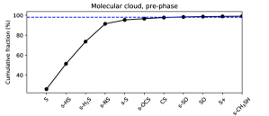
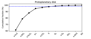
Figure 8: Cumulative sulfur abundance fraction of the ten main sulfur carriers from Nautilus models. Top: molecular cloud. Bottom: AB Aur protoplanetary disk at r=200 au. The horizontal blue dashed line depicts the position of the 98% cumulative fraction.

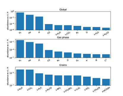
Figure 9: Abundances of the ten most abundant species in our Nautilus model for the global content (top), the gas phase (middle), the surface of grains (bottom).

In Fig. 9 we show the 10 most abundant species for the different phases of the model, as well as for the global case. Surface H2S is the third most abundant species, after g-H2O and g-CO. Furthermore, considering all phases (Fig. 9, top left) g-H2S is the ninth most abundant species in the model. This makes H2S a relevant component of dust grains, whose abundance in different protoplanetary systems is worth modeling.

In Fig. 10, top panel, we show the vertical profile at r=200 au of a few sulfur carriers that are important for the sulfur budget in the gas phase, namely: H2S, CS, SO, and SO2. This figure helps us to identify at which height over the mid-plane the emission of the different species originates. Before z$\rm\sim,$ 7 au the height profiles of the four species remain mostly flat at low abundances. At 7 au, their abundances start to grow, and SO, and SO2 peak around 13 au, while CS peaks at 15 au. The H2S vertical profile forms a high abundance plateau that extends from $\rm\sim$10 to $\rm\sim$15 au where the abundance reaches values of a few $\rm 10^{-9}$. The plateau is preceded by a dip where the abundance goes down by three orders of magnitude. In the bottom panel of Fig. 10 we show the same as in the top panel, but this time for the different phases of H2S: gas phase and H2S in the surface of grains (g-H2S). At low heights over the mid-plane (high extinction), the dominant phase is H2S on the surface of grains.

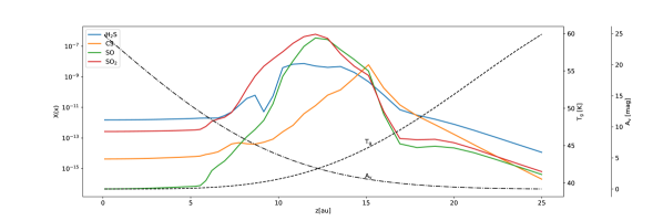
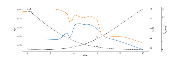
Figure 10: Vertical profiles at r=200 au. Top: of important sulfur carriers in the gas phase, namely H2S, CS, SO, and SO2. Bottom: of H2S in the gas phase and in the surface of grains (g-).We also include the vertical profile of $\rm A_{v}$ and $\rm T_{g}$ for comparison.

4.3 Parameter impact

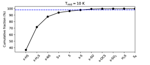
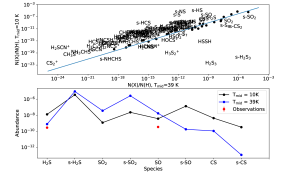
Figure 11: Impact of varying the mid-plane temperature on the model results. Top: cumulative sulfur abundance fraction of the ten main sulfur carriers for the Nautilus model with $\rm T_{mid}$=10 K. Middle: abundance of sulfuretted species computed assuming $\rm T_{mid}$=10 K versus the abundance computed assuming $\rm T_{mid}$=39 K. We show the names of the species when there is an order of magnitude difference between both models, and plot black dots otherwise. Bottom: abundance of a subset of the most relevant sulfur carriers for the two mid-plane temperatures used.

In the following subsection, we discuss the impact of changing key model parameters on the results. The first parameter whose impact we wanted to test is the temperature of the mid-plane. To that aim, we computed a model with a mid-plane temperature of 10 K, compared to 39 K assumed in the previous model (see Table 1). The cumulative sulfur abundance fraction of the ten most relevant sulfur carriers from this model is shown in the top panel of Fig. 11. The most relevant sulfur carrier for the model with $\rm T_{mid}=10$ K is g-HS, it is not in the list of the 10 most relevant sulfur carriers in the model with $\rm T_{mid}=39$ K. The same happens with a g-NS, which are among the most relevant sulfur carriers in the $\rm T_{mid}=10\leavevmode\nobreak\ K$ model. Species that are important sulfur carriers in the main model ($\rm T_{mid}=39\leavevmode\nobreak\ K$) are irrelevant to the sulfur budget in the $\rm T_{mid}=10\leavevmode\nobreak\ K$ model. Such species include g-SO2 and g-H2S3. We show in the middle of Fig. 11 a comparison of the abundances of all the sulfuretted species from the model with $\rm T_{mid}=10$ K versus the abundances from the model with $\rm T_{mid}=39$ K. The figure presents a large scatter, indicating that varying the temperature of the mid-plane gas has an important impact on the derived sulfur abundances. In the bottom panel of Fig. 11 we show the abundances of a subset of important sulfur carriers. While the differences are small for H2S in the surface and mantle of grains, they are large for all the other species represented. We include in the bottom panel the abundances derived from our observations assuming LTE. As can be seen, none of the models matches the two observed species, but the main model provides a good fit for H2S. In the middle panel of Fig. 11 we see that some molecules show differences of several orders of magnitude. Therefore, a subset of these species can be used to get insight into the mid-plane temperature, according to models.

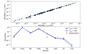
Figure 12: Impact of varying the prephase temperature on the model results. Top: abundance of sulfuretted species computed assuming $\rm T_{gas}$=10 K versus the abundance computed assuming $\rm T_{gas}$=18 K for the molecular cloud prephase. Bottom: abundance of a subset of the most relevant sulfur carriers for the two prephase temperatures used.

The second parameter that we wanted to test is the temperature of the cold cloud prephase. To that aim, we computed a model using a prephase with a temperature of 18 K. As can be seen in Fig. 12 the differences between the two models are not relevant, and a change in the prephase gas temperature will produce almost the same results, especially in the gas phase.

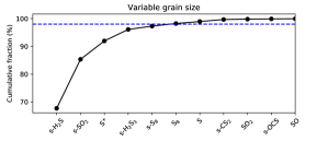
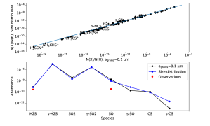
Figure 13: Impact of varying grain size on the model results. Top: cumulative sulfur abundance fraction of the ten main sulfur carriers for the Nautilus model computed assuming a grain size distribution. Middle: abundance of sulfuretted species computed assuming $\rm a_{grains}$=0.1 $\rm\mu m$ versus the abundance computed assuming a grain size distribution. We show the names of the species when there is an order of magnitude difference between both models, and plot black dots otherwise.Bottom: abundance of a subset of the most relevant sulfur carriers for the model with fixed grain size and with a distribution of sizes.

We also tested the impact of a varying grain size distribution. To that aim, we assumed a different grain size at each height, with 1 mm grains in the mid-plane, 0.1 $\rm\mu$ m in the atmosphere, and a logarithmic interpolation in between. We use the same dust temperature in both models. We show in Fig. 13 the results from this model versus the original model results. While the difference is not as large as when changing the mid-plane temperature, the impact of grain sizes cannot be ignored. As can be seen in the top panel of Fig. 13, the species that dominate the sulfur budget are similar to those in the case of the original model (Fig. 8). However, although the grain size distribution affects the results, those for the gaseous species tracked in the bottom panel of Fig. 13 remain mostly unchanged.

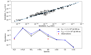
Figure 14: Impact of varying the UV flux on the model results. Top: cumulative sulfur abundance fraction of the ten main sulfur carriers for the Nautilus model computed assuming $\rm f_{UV}$=12. Middle: abundance of sulfuretted species computed assuming $\rm f_{UV}$=12 Draine unit versus the abundance computed assuming $\rm f_{UV}$=1.2$\rm\times 10^{4}$ Draine units. Bottom: abundance of a subset of the most relevant sulfur carriers for the model with $\rm f_{UV}$=12 Draine unit and with $\rm f_{UV}$=1.2$\rm\times 10^{4}$ Draine units.

Finally, we tested the impact of the UV field by computing a model with a meager value of the scale factor of the UV flux, $\rm f_{UV}=12$, compared to $\rm f_{UV}=12\times 10^{4}$ in the main model (see Table 1). We show in Fig. 14 a comparison between the two models. The impact on the abundances is small, and only a few species show a difference larger than one order of magnitude. One of those species is S⁺, which drops by more than one order of magnitude when a low UV flux is assumed.

Table 4: Comparison of abundances in different environments

Species	AB Aur	GG Tau	Horsehead PDR	TMC 1-CP	Orion KL
H2S	2.4$\rm\times 10^{-10}$	1.8$\rm\times 10^{-10}$∗	3.3$\rm\times 10^{-10}$	$\rm 1.1\times 10^{-9}$	1.5$\rm\times 10^{-6}$
SO	3.2$\rm\times 10^{-9}$	–	3.9$\rm\times 10^{-10}$	$\rm 1.0\times 10^{-9}$	8$\rm\times 10^{-8}$
CS	2.6$\rm\times 10^{-10}$∗	3.1$\rm\times 10^{-10}$∗	4.5$\rm\times 10^{-10}$	$\rm 1.3\times 10^{-8}$	7$\rm\times 10^{-8}$
S budget	$\rm>9.2\times 10^{-10}$	$\rm>4.9\times 10^{-10}$	$\rm>1.2\times 10^{-9}$	$\rm>1.5\times 10^{-8}$	$\rm>1.7\times 10^{-6}$
S budget†	–	–	$\rm 1.5\times 10^{-9}$	–	$\rm 1.9\times 10^{-6}$

5 Discussion

The detection of H2S emission in a ring around AB Aur is the second resolved observation of H2S in a protoplanetary disk, after the detection toward GG Tau by Phuong et al. (2018), and the sixth detection after the four single dish detections in Taurus protoplanetary disk (Rivière-Marichalar et al. 2021).

Assuming LTE we derived a mean column density of (1.9$\rm\pm$0.4)$\rm\times 10^{13}\leavevmode\nobreak\ cm^{-2}$ and a mean abundance with respect to ¹³CO of (1.5$\rm\pm$0.4)$\rm\times 10^{-4}$. By assuming $\rm{}^{12}CO$/$\rm{}^{13}CO$=60, and X($\rm{}^{12}CO$)=10^-4, we converted the abundance with respect to $\rm{}^{13}CO$ to an abundance with respect to H₂, resulting in a mean value of (2.4$\rm\pm$0.6)$\rm\times 10^{-10}$. The region surrounding the dust trap depicts the maximum H2S abundance in the disk. Our Nautilus 1D model from Sect. 4 predicts N(H2S)=3.5$\rm\times 10^{13}$ (X(H2S)=7.5$\rm\times 10^{-10}$), about two times larger than the value that we estimate assuming LTE. Using the same methodology, we derived the SO column density from our SO 5₆-4₅ NOEMA observations from Rivière-Marichalar et al. (2020), resulting in a mean SO column density of 1.0$\rm\times 10^{14}\leavevmode\nobreak\ cm^{-2}$, resulting in a mean abundance of 3.2$\rm\times 10^{-9}$, $\rm\sim$2.4 times smaller than the value predicted by our Nautilus model, N(SO)=7.8$\rm\times 10^{14}$ (X(SO)=9.8$\rm\times 10^{-9}$). Recently, CCS was detected toward GG Tau (Phuong et al. 2021). The authors could not simultaneously reproduce the observed column density of CCS and other sulfuretted species, supporting the idea that astrochemical sulfur networks are incomplete. The complexity of simultaneously predicting the abundance of important sulfur carriers such as CS, SO, SO₂, and H₂S is a known issue of sulfur chemistry networks in astrochemical models (Navarro-Almaida et al. 2020). Sulfur astrochemical networks have improved over the last years (Le Gal et al. 2017; Vidal et al. 2017; Navarro-Almaida et al. 2020), with new formation and destruction routes. Yet, progress is needed to solve the issue. However, the goal of the model is not to reproduce the observed values, but rather to get insight into the main sulfur carriers. Furthermore, considering the uncertainties in the model, related to the physical structure and the details of the chemical network, we consider that the model results in a good fit of the H2S line.

From the computed column density map we derived a mean H2S abundance with respect to $\rm{}^{13}CO$ of $\rm(1.5\pm 0.4)\times 10^{-4}$. Assuming a $\rm{}^{12}CO$ abundance of 10^-4 and $\rm{}^{12}CO$/$\rm{}^{13}CO$=60, we derived a mean abundance with respect to H nuclei X(H2S)=(2.4$\rm\pm$0.6)$\rm\times 10^{-10}$. To help us with the discussion we also derived abundances for SO, the other sulfuretted species that we observed toward AB Aur (Rivière-Marichalar et al. 2020). The mean SO abundance with respect to $\rm{}^{13}CO$ is $\rm(1.9\pm 0.2)\times 10^{-3}$, resulting in an abundance with respect to H nuclei X(SO)=(3.1$\rm\pm$2.3)$\rm\times 10^{-9}$.

In the following, we compare the H2S abundance derived in AB Aur with that derived in different environments. Phuong et al. (2018) used Nautilus to derive a column density for the disk around the M0 star GG Tau N(H2S)=3.4$\rm\times 10^{13}\leavevmode\nobreak\ cm^{-2}$, close to our estimate for AB Aur. Rivière-Marichalar et al. (2021) detected H2S in four young stellar objects in Taurus, with column densities in the range 3.2$\rm\times 10^{12}\leavevmode\nobreak\ cm^{-2}$ to 1.9$\rm\times 10^{13}\leavevmode\nobreak\ cm^{-2}$. This set of values was computed for a disk with an outer radius of 500 au. However, this size is larger than the H2S disk observed toward AB Aur. If an outer radius of 250 au is assumed, the computed column densities are in the range $\rm 10^{13}\leavevmode\nobreak\ cm^{-2}$ to 7$\rm\times 10^{13}\leavevmode\nobreak\ cm^{-2}$, close to the value derived for AB Aur. The difference in spectral type does not impact the individual column densities. Since H2S has been detected only in a few protoplanetary disks, no statistical trend can be derived, but the proximity between observed abundances is interesting.

The abundance derived for AB Aur is four orders of magnitude lower than that found in the Orion KL hot core (1.5 $\rm\times 10^{-6}$, Esplugues et al. 2014), but similar to that found in two PDRs, the Horsehead nebula (3.1$\rm\times 10^{-10}$, Rivière-Marichalar et al. 2019a) and the Orion Bar (4.0$\rm\times 10^{-10}$, Leurini et al. 2006). This is particularly interesting because H2S presents almost the same abundance in very different PDRs (the Horsehead with a radiation intensity of G$\rm{}_{0}\sim 10^{2}$ and the Orion Bar, a much more extreme PDR with G₀=$\rm 10^{4}$. Overall, the chemical abundances in PDRs are governed by the ratio of the UV radiation field and the density ($\rm G_{0}/n_{H}$). In the case of H2S, this species is mainly formed on grain surfaces and later released into the gas phase through photodesorption in regions dominated by high UV radiation (Jiménez-Escobar & Muñoz Caro 2011; Jiménez-Escobar et al. 2014; Fuente et al. 2017a). The high UV radiation is also responsible for the destruction of H2S through dissociation processes. The interplay between formation and destruction mechanisms makes the position of the H2S abundance peak roughly independent of G₀. This is partially confirmed by our experiment with a low-UV model, which results in very close H2S abundances: 6.9$\rm\times 10^{-10}$ for the model with a low UV field versus 7.5$\rm\times 10^{-10}$ for the model with high UV field.

Regarding density, it has a crucial role in the H2S abundance, since both the formation of solid H2S on the surface of grains and its desorption depend on the density of the region. In particular, solid H2S is mainly formed through recombination of S⁺ ions (formed as the UV photons penetrate the gas ionizing S atoms) with negatively charged grains followed by desorption. Adsorption of S⁺ is favored in dense regions by the increased collision rates between gas-phase species and grains (Gail & Sedlmayr 1975; Bel et al. 1989; Ruffle et al. 1999; Druard & Wakelam 2012). Once that solid H2S is formed, the H2S photodesorption rates depend on the grain size distribution, which in turn depends on $\rm n_{H}$. This implies that, for a given radiation field, the H2S abundance peak will be shifted toward the densest part of a PDR as theoretically found by Goicoechea et al. (2021).

The huge change in the abundance of H2S in the gas phase from hot cores to Class II disks and PDRs points to H2S being an important sulfur carrier in the icy surface of dust grains, such that it is almost fully evaporated in hot cores, thus increasing the fraction of gas-phase H2S. This is confirmed by our Nautilus model from Sect. 4, where only $\rm\sim$ 0.0001% of H2S is in gas phase. In this model, a large fraction ($\rm\sim$61%) of the cosmic sulfur abundance is locked in the surface and mantle of grains in the form of H2S, and another 17% is also locked in the surface and mantle of grains in the form of SO2. The low sulfur abundances observed in AB Aur and other protoplanetary disks (Le Gal et al. 2019) can indeed be explained if sulfur is locked in the ice surface of dust grains, similar to what happens in dense cores (Millar & Herbst 1990; Ruffle et al. 1999; Vidal et al. 2017; Laas & Caselli 2019). Laas & Caselli (2019), using a chemical network with 860 species, showed that most sulfur is locked on dust grains and that grain chemistry could account for the depleted sulfur in molecular clouds. Our 1D protoplanetary disk model shows a similar result, with most of the sulfur locked in the surface of dust grains in the form of H2S, SO2 and H2S3 at high extinctions, and dominated by S⁺ at low extinctions.

We note that our results for the sulfur budget depend on the chemical network used, as well as on the details of the model. For instance, in the molecular cloud model by Laas & Caselli (2019) the amount of H2S in ices is negligible for most of the cloud’s life. The chemical network used in Laas & Caselli (2019) is different from the one we used in the present paper, and their model does not include a mantle phase, which results in very different abundances of H2S on the surface of grains. We highlight, however, that H2S is the most abundant sulfuretted species in comets (Bockelée-Morvan & Biver 2017), in agreement with our results.

Cazaux et al. (2022) find that, under efficient self-shielding conditions, H2S survives on the surface of grains as the ice below 100 K, and is largely depleted from the grains at 150 K. However, if no self-shielding is assumed, most H2S is transformed, under the influence of UV radiation, into S_x sulfur chains. Our Nautilus model predicts that gaseous S₈ and that the surface of grains is the seventh and eighth major sulfur carrier.

6 Summary and conclusions

In this study we present resolved observations of H2S $\rm 1_{01}-1_{10}$ in AB Aur. This is only the second time that H2S has been resolved in a protoplanetary disk, and the sixth global detection. The main results from our study can be summarized as follows:

1. We detected o-H2S $\rm 1_{01}-1_{10}$ in a ring extending from $\rm\sim$0.67$\rm\arcsec$ ($\rm\sim$109 au) to 1.69$\rm\arcsec$ ($\rm\sim$275 au). We observed strong azimuthal asymmetries. The position of the peak coincides with the position of the continuum and C¹⁸O emission peaks. The radial profile of the emission overlaps with that of H2CO.

2. Assuming LTE, we estimated a mean column density of $\rm(1.9\pm 0.4)\times 10^{13}\leavevmode\nobreak\ cm^{-2}$. Making simple assumptions, we translated this column density into an abundance of (2.4$\rm\pm$0.6)$\rm\times 10^{-10}$.

3. A Nautilus 1D model shows that most (99.99%) of the H2S is locked in the surface of dust grains. The model also shows that they are the main sulfur carriers. Our model further shows that $\rm\sim$90.5% of the sulfur is locked on the surface of grains, and only 9.5% of it is available in the gas phase.

Our study of the sulfur budget in the protoplanetary disk surrounding AB Aur points to H2S being the most important sulfur carrier on the surface of grains. Furthermore, it is the third most abundant species on the surface of grains, after H2O and CO2. Our results probe that H2S observations are an essential diagnostic to determine the sulfur depletion in protoplanterary disks. Observations of H2S and other sulfuretted species toward more young stellar objects are needed to understand sulfur depletion and put our observations of AB Aur in context.