Massive form factors at $\mathcal{O}(\alpha_{s}^{3})$

Abstract

We report on our recent calculation of massive quark form factors using a semi-numerical approach based on series expansions of the master integrals around singular and regular kinematic points and numerical matching. The methods allows to cover the whole kinematic range of negative and positive values of the virtuality $s$ with at least seven significant digits accuracy.

1 Introduction

Massive form factors are important objects in quantum field theory. They constitute the virtual corrections to many observables and processes like lepton pair production via the Drell-Yan process or the decay of the Higgs boson into heavy quarks. The more and more precise measurements of these processes make the inclusion of higher order corrections for the theory predictions necessary.

Up to $\mathcal{O}(\alpha_{s}^{2})$ the massive form factors are known in analytic form, see Refs. [1, 2, 3, 4, 5, 6, 7], and even higher orders in the dimensional regulator $\epsilon$ haven been considered in Refs. [8, 9, 10, 11, 12]. At $\mathcal{O}(\alpha_{s}^{3})$ only partial results are available. At this order the form factors have been considered in the large-$N_{C}$ limit (with $N_{C}$ the number of colors) in Refs. [9, 13, 14, 15], the light fermion contributions were calculated in Ref. [12] and in Ref. [16] all non-singlet contributions involving a closed heavy quark loop have been considered.

In these proceedings we report on our recent calculation of the massive form factors at $\mathcal{O}(\alpha_{s}^{3})$ in Refs. [17, 18], where we employed a semi-numerical method involving series expansions and numerical matching between them. In Section 2 we will summarize technical details, while in Section 3 we show some results. In Section 4 we conclude and give an outlook.

2 Massive form factors

To compute the massive form factors we consider the interaction of a massive quark with a vector, axial-vector, scalar or pseudo-scalar current, which are given by:

$$j_{\mu}^{v} = \bar{\psi}\gamma_{\mu}\psi\,,$$

$$j_{\mu}^{a} = \bar{\psi}\gamma_{\mu}\gamma_{5}\psi\,,$$

$$j^{s} = m\,\bar{\psi}\psi\,,$$

$$j^{p} = \text{i}m\,\bar{\psi}\gamma_{5}\psi\,.$$ (1)

The vertex function can then be expressed through six scalar functions by

$$\Gamma_{\mu}^{v}(q_{1},q_{2}) = F_{1}^{v}(q^{2})\gamma_{\mu}-\frac{\text{i}}{2m}F_{2}^{v}(q^{2})\sigma_{\mu\nu}q^{\nu}\,,$$

$$\Gamma_{\mu}^{a}(q_{1},q_{2}) = F_{1}^{a}(q^{2})\gamma_{\mu}\gamma_{5}{-\frac{1}{2m}F_{2}^{a}(q^{2})q_{\mu}}\gamma_{5}\,,$$

$$\Gamma^{s}(q_{1},q_{2}) = {m}F^{s}(q^{2})\,,$$

$$\Gamma^{p}(q_{1},q_{2}) = {\text{i}m}F^{p}(q^{2}){\gamma_{5}}\,.$$ (2)

Here the momentum $q_{1}$ ($q_{2}$) is incoming (outgoing), on-shell ($q_{1}^{2}=q_{2}^{2}=m^{2}$) and $q=q_{1}-q_{2}$ is the outgoing momentum at the current $j^{\delta}$ with $q^{2}=s$. The form factors have an expansion in the strong coupling constant $\alpha_{s}$

$$F_{i}^{j}=\sum\limits_{l}\left(\frac{\alpha_{s}}{\pi}\right)^{l}F_{i}^{j,(l)}~{}.$$

We divide the form factor into non-singlet and singlet contributions, where the current couples to the heavy external quark line or an internal heavy quark loop, respectively. Some sample Feynman diagrams contributing to the form factors can be found in Fig. 1.

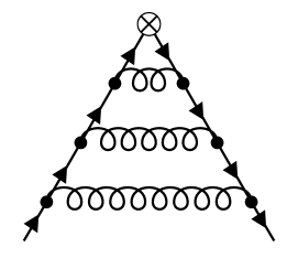
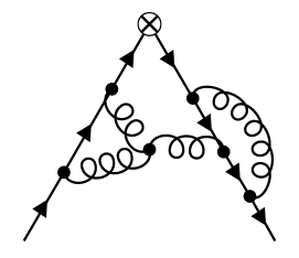
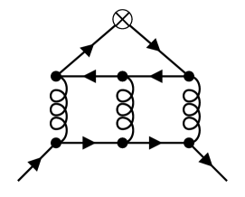
Figure 1: Sample Feynman diagrams contributing to the massive quark form factors. Solid lines represent massive quark, while curly lines represent gluons. The vertex with a cross refers to the coupling to one of the external currents. The diagram on the right is part of the singlet contributions.

The calculation of the form factors proceeds in the following way: We generate the diagrams with QGRAF [19] and use q2e [20, 21] to transform the output to FORM [22] input, where Dirac-, Lorenz- and color-algebra (with color [23]) is performed. The diagrams are mapped to predefined topologies using exp [20, 21]. The scalar integrals are reduced to master integrals with the help of Kira [24, 25] with Fermat [26] on a family-by-family basis. We make sure to reduce to a basis where the dependence on $d$ and the kinematic variable $s$ factorizes utilizing an improved version of ImproveMasters, first developed in Ref. [27]. Afterwards we symmetrize over all families and find 422 master integrals for the non-singlet contribution and 316 for the singlet diagrams. In a next step, we set up a systems of differential equations for the master integrals in the variable $\hat{s}=s/m^{2}$ by calculating the derivatives with the help of LiteRed [28, 29] and subsequent reduction with Kira.

Subsequently, the master integrals need to be solved. This is achieved using the semi-numerical approach presented in Ref. [30] and explained in more detail for the current problem in Ref. [18]. Let us summarize the main ideas of the approach:

1. We calculate boundary conditions for all master integrals at the special point $s=0$. At this special point the master integrals in the non-singlet case reduce to three-loop on-shell propagators, which are well studied in the literature [31, 32, 33]. However, we needed to extend the depth of the $\epsilon$ expansion, since we encountered high spurious poles in the amplitude after reducing to master integrals. The results can be found in Ref. [18]. Since the singlet diagrams have massless cuts, we need to perform an asymptotic expansion around $s=0$ to obtain their boundary conditions.

2. We calculate symbolic expansions around the point $s=0$ by inserting a suitable ansatz into the system of differential equations. By comparing powers in $\epsilon$, the expansion parameter $s$ and possibly logarithms of the expansion parameter, we obtain a system of linear equations for the coefficients of the ansatz. We solve this system of equations with Kira and FireFly [34, 35] in terms of a small set of boundary conditions, which can be determined from step 1.

3. We calculate symbolic expansions around a new point $s_{1}$ and match the two expansions numerically at a point where both expansions converge, e.g. $s_{1}/2$.

4. Afterwards, we generate another symbolic expansion at $s_{2}$ and match it to the expansion around $s_{1}$ at a point where both expansions converge. This way we can map out the whole kinematics of the process.

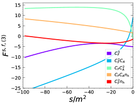
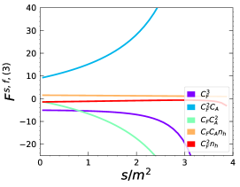
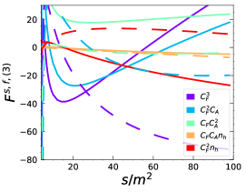
Figure 2: The UV-renormalized and infrared subtracted form factor $F^{s,f,(3)}$. Solid lines correspond to the real part, dashed lines to the imaginary part of the corresponding color factor. Taken from Ref. [18].

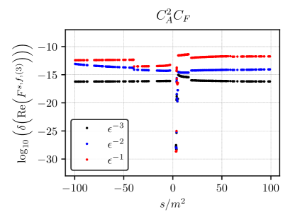
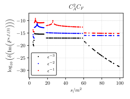
Figure 3: Relative cancellation of the real (left) and imaginary part (right) of the poles for the color factor $C_{F}C_{A}^{2}$ of $F^{s,f,(3)}$. Taken from Ref. [18].

3 Results

The main results of our method are overlapping series expansions which can be used to evaluate the massive form factors at any value of $s$. In Fig. 2 we show as an example the non-singlet contributions to the form factor $F^{s}$, where the masses and wave function are renormalized on-shell, the current in the $\overline{\rm MS}$-scheme and the remaining infrared divergencies are subtracted by multiplying with a suitably defined $Z$-factor, which can be constructed from the cusp anomalous dimension [36, 37, 38, 39] (see Refs. [9, 18] for the precise definition). The resulting finite form factors are labeled with an additional superscript $f$. Note, that our expansion around $s=0$ is analytic, e.g. for $F^{s,f,(3)}$, i.e. the non-singlet contribution to the scalar form factor, we find:

$$F^{s,f,(3)}\Big{|}_{s\to 0}=C_{A}C_{F}^{2}\Bigg{[}\frac{4a_{4}}{3}+\frac{491\zeta_{3}}{96}+\frac{19\pi^{2}\zeta_{3}}{16}-\frac{45\zeta_{5}}{16}+\frac{26117}{4608}-\frac{1193\pi^{2}}{576}-\frac{65\pi^{4}}{432}+\frac{l_{2}^{4}}{18}$$

$$\quad+\frac{31}{36}\pi^{2}l_{2}^{2}+\frac{43}{18}\pi^{2}l_{2}\Bigg{]}+C_{A}^{2}C_{F}\Bigg{[}-\frac{11a_{4}}{3}-\frac{947\zeta_{3}}{288}-\frac{51\pi^{2}\zeta_{3}}{64}+\frac{65\zeta_{5}}{32}-\frac{584447}{124416}+\frac{3011\pi^{2}}{3456}$$

$$\quad+\frac{179\pi^{4}}{3456}-\frac{11l_{2}^{4}}{72}-\frac{11}{36}\pi^{2}l_{2}^{2}+\frac{49}{72}\pi^{2}l_{2}\Bigg{]}+C_{F}^{3}\Bigg{[}12a_{4}+\frac{87\zeta_{3}}{16}+\frac{\pi^{2}\zeta_{3}}{16}-\frac{5\zeta_{5}}{8}+\frac{55}{96}+\frac{643\pi^{2}}{192}$$

$$\quad+\frac{\pi^{4}}{48}+\frac{l_{2}^{4}}{2}-\frac{1}{2}\pi^{2}l_{2}^{2}-\frac{15}{2}\pi^{2}l_{2}\Bigg{]}+C_{F}^{2}T_{F}n_{h}\Bigg{[}8a_{4}+\frac{17\zeta_{3}}{18}-\frac{2083}{432}-\frac{52\pi^{2}}{81}-\frac{\pi^{4}}{720}+\frac{l_{2}^{4}}{3}$$

$$\quad-\frac{1}{3}\pi^{2}l_{2}^{2}+\frac{8}{9}\pi^{2}l_{2}\Bigg{]}+C_{F}C_{A}T_{F}n_{h}\Bigg{[}-6a_{4}-\frac{199\zeta_{3}}{144}+\frac{\pi^{2}\zeta_{3}}{8}-\frac{5\zeta_{5}}{8}+\frac{209857}{15552}-\frac{4351\pi^{2}}{1296}$$

$$\quad-\frac{\pi^{4}}{288}-\frac{l_{2}^{4}}{4}+\frac{1}{4}\pi^{2}l_{2}^{2}+\frac{32}{9}\pi^{2}l_{2}\Bigg{]}$$

$$\quad+\frac{s}{m^{2}}\Bigg{\{}C_{A}C_{F}^{2}\Bigg{[}-\frac{8a_{4}}{9}+\frac{2515\zeta_{3}}{2304}-\frac{29\pi^{2}\zeta_{3}}{144}-\frac{95\zeta_{5}}{48}+\frac{11191}{41472}-\frac{15101\pi^{2}}{62208}+\frac{37\pi^{4}}{4320}-\frac{l_{2}^{4}}{27}$$

$$\quad+\frac{1259\pi^{2}l_{2}^{2}}{2160}+\frac{1409\pi^{2}l_{2}}{1440}\Bigg{]}+C_{A}^{2}C_{F}\Bigg{[}\frac{5a_{4}}{4}+\frac{8675\zeta_{3}}{10368}-\frac{73\pi^{2}\zeta_{3}}{1152}+\frac{125\zeta_{5}}{384}-\frac{851465}{279936}$$

$$\quad+\frac{130417\pi^{2}}{186624}+\frac{689\pi^{4}}{103680}+\frac{5l_{2}^{4}}{96}-\frac{1}{20}\pi^{2}l_{2}^{2}-\frac{12253\pi^{2}l_{2}}{8640}\Bigg{]}+C_{F}^{3}\Bigg{[}-\frac{29a_{4}}{9}-\frac{12401\zeta_{3}}{3456}$$

$$\quad-\frac{67\pi^{2}\zeta_{3}}{288}+\frac{85\zeta_{5}}{32}+\frac{22613}{41472}-\frac{69355\pi^{2}}{31104}+\frac{1727\pi^{4}}{25920}-\frac{29l_{2}^{4}}{216}-\frac{1043\pi^{2}l_{2}^{2}}{1080}+\frac{4013\pi^{2}l_{2}}{1080}\Bigg{]}$$

$$\quad+C_{F}^{2}T_{F}n_{h}\Bigg{[}\frac{8a_{4}}{9}+\frac{9889\zeta_{3}}{6912}-\frac{8059}{5184}-\frac{4261\pi^{2}}{25920}+\frac{7\pi^{4}}{1620}+\frac{\log^{4}(2)}{27}-\frac{1}{27}\pi^{2}l_{2}^{2}+\frac{4}{27}\pi^{2}l_{2}\Bigg{]}$$

$$\quad+C_{F}C_{A}T_{F}n_{h}\Bigg{[}-\frac{5a_{4}}{18}+\frac{1657\zeta_{3}}{1728}+\frac{\pi^{2}\zeta_{3}}{96}+\frac{5\zeta_{5}}{96}+\frac{2257}{3888}-\frac{13663\pi^{2}}{25920}-\frac{121\pi^{4}}{51840}-\frac{5l_{2}^{4}}{432}$$

$$\quad+\frac{5}{432}\pi^{2}l_{2}^{2}+\frac{55}{108}\pi^{2}l_{2}\Bigg{]}\Bigg{\}}+{\cal O}\left(\frac{s^{2}}{m^{4}}\right)+\mbox{$n_{l}$, $n_{l}^{2}$ and $n_{h}^{2}$ terms},$$ (3)

where $l_{2}=\log(2)$, $a_{4}=\mbox{Li}_{4}(1/2)$ and $\zeta_{n}$ is Riemann’s zeta function evaluated at $n$ and $C_{F}=T_{F}(N_{C}^{2}-1)/N_{C}$, $C_{A}=2T_{F}N_{C}$ are the quadratic Casimir operators of the ${\rm SU}(N_{C})$ gauge group in the fundamental and adjoint representation, respectively, $n_{l}$ is the number of massless quark flavors, $n_{h}$ is the number of heavy quark flavors with mass $m$ and $T_{F}=1/2$.

There are several checks on our results. For example, the coefficient in front of the gauge parameter in the final result is smaller than $10^{-18}$ and we can reproduce the known analytic results in the planar limit, the contributions $\sim n_{l}$ and the $n_{h}^{2}$ contributions with at least 12 digits. Furthermore, the results are precise enough to calculate the leading and sub-leading logarithmic corrections in the high energy expansion for the first power suppressed contributions analytically. These corrections have been obtained in Refs. [40, 41, 42, 43] by considering an involved asymptotic expansion of the Feynman diagrams. We find agreement except of the quartic mass suppressed corrections to the form factor $F_{2}^{v,(3)}$. Our results have been confirmed by the authors of Ref. [43]. More details and analytic expressions for several expansion terms can be found in Ref. [18].

The precision of our final results can be estimated from the cancellation of the poles in the dimensional regulator $\epsilon$, since they are known analytically and have to cancel in the final result. We use the logarithm to the base 10 of the relative pole cancellation (denoted by $\delta$) as a measure of accurate digits. A plot of this measure for the form factor $F^{s,f,(3)}$ and the color factor $C_{F}C_{A}^{2}$, split into real and imaginary part, can be found in Fig. 3. We see that the precision for $s<3$ and $s>16$ is highest and decreases for the regions between the two thresholds at $s=4m^{2}$ (two particle threshold) and $s=16m^{2}$ (three particle threshold), which are not analytic. In total we estimate at least 7 significant digits over the whole kinematic range for all of our results. The results of the singlet contributions is significantly higher and estimated to be at least 10 digits.

A Mathematica package to evaluate the form factors in the non-singlet and singlet case numerically over the full kinematic range of $s$ can be found at:

https://gitlab.com/formfactors3l/formfactors3l.

4 Conclusions and Outlook

We presented our recent calculation of massive quark form factors at $\mathcal{O}(\alpha_{s}^{3})$ which uses a semi-numerical method based on series expansions and numerical matching to obtain results for the form factors for the whole kinematic range of negative and positive values of the virtuality $s$. We obtain a precision of at least 7 significant digits in the non-singlet and 10 digits in the singlet case over the whole kinematic range, respectively. However, some kinematic regions are much more precise. Thus, it is for example possible to extract leading and sub-leading logarithmic contributions to the leading and first power suppressed terms in the high energy expansion analytically, confirming and correcting results in the literature. To complete the calculation of massive quark form factors the singlet diagrams where the external current couples to an internal light quark loop still need to be completed.

References

- [1] A.H. Hoang and T. Teubner, Analytic calculation of two loop corrections to heavy quark pair production vertices induced by light quarks, Nucl. Phys. B 519 (1998) 285 [hep-ph/9707496].
- [2] P. Mastrolia and E. Remiddi, Two loop form-factors in QED, Nucl. Phys. B 664 (2003) 341 [hep-ph/0302162].
- [3] R. Bonciani, P. Mastrolia and E. Remiddi, QED vertex form-factors at two loops, Nucl. Phys. B 676 (2004) 399 [hep-ph/0307295].
- [4] W. Bernreuther, R. Bonciani, T. Gehrmann, R. Heinesch, T. Leineweber, P. Mastrolia et al., Two-loop QCD corrections to the heavy quark form-factors: The Vector contributions, Nucl. Phys. B 706 (2005) 245 [hep-ph/0406046].
- [5] W. Bernreuther, R. Bonciani, T. Gehrmann, R. Heinesch, T. Leineweber, P. Mastrolia et al., Two-loop QCD corrections to the heavy quark form-factors: Axial vector contributions, Nucl. Phys. B 712 (2005) 229 [hep-ph/0412259].
- [6] W. Bernreuther, R. Bonciani, T. Gehrmann, R. Heinesch, T. Leineweber and E. Remiddi, Two-loop QCD corrections to the heavy quark form-factors: Anomaly contributions, Nucl. Phys. B 723 (2005) 91 [hep-ph/0504190].
- [7] W. Bernreuther, R. Bonciani, T. Gehrmann, R. Heinesch, P. Mastrolia and E. Remiddi, Decays of scalar and pseudoscalar Higgs bosons into fermions: Two-loop QCD corrections to the Higgs-quark-antiquark amplitude, Phys. Rev. D 72 (2005) 096002 [hep-ph/0508254].
- [8] J. Gluza, A. Mitov, S. Moch and T. Riemann, The QCD form factor of heavy quarks at NNLO, JHEP 07 (2009) 001 [0905.1137].
- [9] J. Henn, A.V. Smirnov, V.A. Smirnov and M. Steinhauser, Massive three-loop form factor in the planar limit, JHEP 01 (2017) 074 [1611.07535].
- [10] T. Ahmed, J.M. Henn and M. Steinhauser, High energy behaviour of form factors, JHEP 06 (2017) 125 [1704.07846].
- [11] J. Ablinger, A. Behring, J. Blümlein, G. Falcioni, A. De Freitas, P. Marquard et al., Heavy quark form factors at two loops, Phys. Rev. D 97 (2018) 094022 [1712.09889].
- [12] R.N. Lee, A.V. Smirnov, V.A. Smirnov and M. Steinhauser, Three-loop massive form factors: complete light-fermion corrections for the vector current, JHEP 03 (2018) 136 [1801.08151].
- [13] R.N. Lee, A.V. Smirnov, V.A. Smirnov and M. Steinhauser, Three-loop massive form factors: complete light-fermion and large-Nc corrections for vector, axial-vector, scalar and pseudo-scalar currents, JHEP 05 (2018) 187 [1804.07310].
- [14] J. Ablinger, J. Blümlein, P. Marquard, N. Rana and C. Schneider, Heavy quark form factors at three loops in the planar limit, Phys. Lett. B 782 (2018) 528 [1804.07313].
- [15] J. Ablinger, J. Blümlein, P. Marquard, N. Rana and C. Schneider, Automated Solution of First Order Factorizable Systems of Differential Equations in One Variable, Nucl. Phys. B 939 (2019) 253 [1810.12261].
- [16] J. Blümlein, P. Marquard, N. Rana and C. Schneider, The Heavy Fermion Contributions to the Massive Three Loop Form Factors, Nucl. Phys. B 949 (2019) 114751 [1908.00357].
- [17] M. Fael, F. Lange, K. Schönwald and M. Steinhauser, Massive Vector Form Factors to Three Loops, Phys. Rev. Lett. 128 (2022) 172003 [2202.05276].
- [18] M. Fael, F. Lange, K. Schönwald and M. Steinhauser, Singlet and non-singlet three-loop massive form factors, 2207.00027.
- [19] P. Nogueira, Automatic Feynman graph generation, J. Comput. Phys. 105 (1993) 279.
- [20] R. Harlander, T. Seidensticker and M. Steinhauser, Complete corrections of Order alpha alpha-s to the decay of the Z boson into bottom quarks, Phys. Lett. B 426 (1998) 125 [hep-ph/9712228].
- [21] T. Seidensticker, Automatic application of successive asymptotic expansions of Feynman diagrams, in 6th International Workshop on New Computing Techniques in Physics Research: Software Engineering, Artificial Intelligence Neural Nets, Genetic Algorithms, Symbolic Algebra, Automatic Calculation, 5, 1999 [hep-ph/9905298].
- [22] B. Ruijl, T. Ueda and J. Vermaseren, FORM version 4.2, 1707.06453.
- [23] T. van Ritbergen, A.N. Schellekens and J.A.M. Vermaseren, Group theory factors for Feynman diagrams, Int. J. Mod. Phys. A 14 (1999) 41 [hep-ph/9802376].
- [24] P. Maierhöfer, J. Usovitsch and P. Uwer, Kira—A Feynman integral reduction program, Comput. Phys. Commun. 230 (2018) 99 [1705.05610].
- [25] J. Klappert, F. Lange, P. Maierhöfer and J. Usovitsch, Integral reduction with Kira 2.0 and finite field methods, Comput. Phys. Commun. 266 (2021) 108024 [2008.06494].
- [26] R.H. Lewis, “Fermat’s user guide.” http://home.bway.net/lewis.
- [27] A.V. Smirnov and V.A. Smirnov, How to choose master integrals, Nucl. Phys. B 960 (2020) 115213 [2002.08042].
- [28] R.N. Lee, Presenting LiteRed: a tool for the Loop InTEgrals REDuction, 1212.2685.
- [29] R.N. Lee, LiteRed 1.4: a powerful tool for reduction of multiloop integrals, J. Phys. Conf. Ser. 523 (2014) 012059 [1310.1145].
- [30] M. Fael, F. Lange, K. Schönwald and M. Steinhauser, A semi-analytic method to compute Feynman integrals applied to four-loop corrections to the -pole quark mass relation, JHEP 09 (2021) 152 [2106.05296].
- [31] S. Laporta and E. Remiddi, The Analytical value of the electron (g-2) at order alpha**3 in QED, Phys. Lett. B 379 (1996) 283 [hep-ph/9602417].
- [32] K. Melnikov and T.v. Ritbergen, The Three loop relation between the MS-bar and the pole quark masses, Phys. Lett. B 482 (2000) 99 [hep-ph/9912391].
- [33] R.N. Lee and V.A. Smirnov, Analytic Epsilon Expansions of Master Integrals Corresponding to Massless Three-Loop Form Factors and Three-Loop g-2 up to Four-Loop Transcendentality Weight, JHEP 02 (2011) 102 [1010.1334].
- [34] J. Klappert and F. Lange, Reconstructing rational functions with FireFly, Comput. Phys. Commun. 247 (2020) 106951 [1904.00009].
- [35] J. Klappert, S.Y. Klein and F. Lange, Interpolation of dense and sparse rational functions and other improvements in FireFly, Comput. Phys. Commun. 264 (2021) 107968 [2004.01463].
- [36] A.M. Polyakov, Gauge Fields as Rings of Glue, Nucl. Phys. B 164 (1980) 171.
- [37] G.P. Korchemsky and A.V. Radyushkin, Renormalization of the Wilson Loops Beyond the Leading Order, Nucl. Phys. B 283 (1987) 342.
- [38] A. Grozin, J.M. Henn, G.P. Korchemsky and P. Marquard, Three Loop Cusp Anomalous Dimension in QCD, Phys. Rev. Lett. 114 (2015) 062006 [1409.0023].
- [39] A. Grozin, J.M. Henn, G.P. Korchemsky and P. Marquard, The three-loop cusp anomalous dimension in QCD and its supersymmetric extensions, JHEP 01 (2016) 140 [1510.07803].
- [40] T. Liu, A.A. Penin and N. Zerf, Three-loop quark form factor at high energy: the leading mass corrections, Phys. Lett. B 771 (2017) 492 [1705.07910].
- [41] T. Liu and A.A. Penin, High-Energy Limit of QCD beyond the Sudakov Approximation, Phys. Rev. Lett. 119 (2017) 262001 [1709.01092].
- [42] T. Liu and A. Penin, High-Energy Limit of Mass-Suppressed Amplitudes in Gauge Theories, JHEP 11 (2018) 158 [1809.04950].
- [43] T. Liu, S. Modi and A.A. Penin, Higgs boson production and quark scattering amplitudes at high energy through the next-to-next-to-leading power in quark mass, JHEP 02 (2022) 170 [2111.01820].
- [44] R.V. Harlander, S.Y. Klein and M. Lipp, FeynGame, Comput. Phys. Commun. 256 (2020) 107465 [2003.00896].