Subgraph Frequency Distribution Estimation
using Graph Neural Networks

Abstract.

Small subgraphs (graphlets) are important features to describe fundamental units of a large network. The calculation of the subgraph frequency distributions has a wide application in multiple domains including biology and engineering. Unfortunately due to the inherent complexity of this task, most of the existing methods are computationally intensive and inefficient. In this work, we propose GNNS, a novel representational learning framework that utilizes graph neural networks to sample subgraphs efficiently for estimating their frequency distribution. Our framework includes an inference model and a generative model that learns hierarchical embeddings of nodes, subgraphs, and graph types. With the learned model and embeddings, subgraphs are sampled in a highly scalable and parallel way and the frequency distribution estimation is then performed based on these sampled subgraphs. Eventually, our methods achieve comparable accuracy and a significant speedup by three orders of magnitude compared to existing methods.

1. Introduction

Network analysis has a wide application in biology (Costa et al., 2011), chemistry (Solé and Munteanu, 2004), engineering (Milo et al., 2002), social science (Juszczyszyn et al., 2008) and communications (Itzkovitz and Alon, 2005). Such analysis is applied in multiple aspects, including studying the distributions of nodes and edges as well as local structure (graphlets and motifs). Although graph mining has a significant impact in multiple domains, most of existing algorithms are extremely computationally intensive and only applicable to small graphs.

In this work, we study a fundamental and important problem in network analysis, to estimate the distribution of subgraphs with the same topology structure given a target graph. Instead of counting the exact number of topology frequency (Hočevar and Demšar, 2014)(Melckenbeeck et al., 2018)(Ribeiro and Silva, 2010b), which involves computing graph isomorphism with a time complexity of NP-complete, we use the idea of sampling to estimate the density of each subgraph type. Different from those traditional sampling-based methods include MFinder (Milo et al., 2002), Monte Carlo Markov Chain (MCMC)-sampling (Saha and Hasan, 2015) etc., we propose GNNS (Graph Neural Network sampling), a novel, fast and scalable learning-based method using graph neural network for sampling. In particular, we utilize the idea of representation learning with a graph variational auto-encoder (VAE), to learn a correlated node embedding with graph convolutions. Then we perform a node-based embedding and extract its connected component as a subgraph. Given that a large mount of subgraphs are sampled independently and simultaneously, our algorithm is highly scalable and parallel. Eventually, our proposed algorithm could achieve a significant speed-up rate with three orders of magnitude with a comparable accuracy compared to the state-of-the-art sampling approach, e.g. MCMC-sampling.

2. Problem Statement

In this section, we present definitions of some fundamental concepts in graph theory that are important for formulating our problem statement. Note we only consider undirected graphs in this paper.

Definition 2.1 (Graph).

Denote $G(V,E)$ as a graph where V is the set of nodes and E the set of edges. Each edge $e\in E$ is denoted by $(u,v)$ where $u\in V$ and $v\in V$.

Definition 2.2 (Subgraph).

A graph $G^{\prime}(V^{\prime},E^{\prime})$ is a subgraph of graph $G(V,E)$ if $V^{\prime}\subseteq V$ and $E^{\prime}\subseteq E$. We then denote this as $G^{\prime}\subseteq G$. If $|V^{\prime}|=k$, we say $G^{\prime}(V^{\prime},E^{\prime})$ is a k-subgraph.

Definition 2.3 (Graph Isomorphism).

Suppose $G_{1}(V_{1},E_{1})$ and $G_{2}(V_{2},E_{2})$ are two graphs. Then $G_{1}(V_{1},E_{1})$ and $G_{2}(V_{2},E_{2})$ are isomorphic if there exists a bijection $f:V_{1}\mapsto V_{2}$ such that $(u,v)\in E_{1}$ if and only if $(f(u),f(v))\in E_{2}$.

Definition 2.4 (Subgraph Type).

Two subgraphs $G_{1}$ and $G_{2}$ of a graph $G$ belong to the same subgraph type $t$ if $G_{1}$ is isomorphic to $G_{2}$.

Definition 2.5 (Frequency (Ribeiro et al., 2021)).

The frequency of a subgraph type $t$ in $G$ is the number of different subgraphs $G^{\prime}$ of G that belong to $t$. Note when counting the frequency, two subgraphs $G^{\prime}(V^{\prime},E^{\prime})$ and $G^{\prime\prime}(V^{\prime\prime},E^{\prime\prime})$ are considered different when either $V^{\prime}\neq V^{\prime\prime}$ or $E^{\prime}\neq E^{\prime\prime}$.

We are now ready to formally define our quantity of interest:

Definition 2.6 ((Normalized) Subgraph Frequency Distribution).

Let ($t_{1},t_{2},...,t_{m}$) be the list of all subgraph types in $G$ that has node number $k$. The k-subgraph frequency distribution is then
$(\frac{n_{1}}{\sum_{i=1}^{m}n_{i}},\frac{n_{2}}{\sum_{i=1}^{m}n_{i}},......,\frac{n_{m}}{\sum_{i=1}^{m}n_{i}})$ where $n_{i}$ is the frequency of $t_{i}$ in $G$.

Here are some other definitions that will be used in our methodology section 4:

Definition 2.7 (Induced Subgraph).

An induced subgraph of graph $G(V,E)$ is a subgraph $G^{\prime\prime}(V^{\prime\prime},E^{\prime\prime})$ where $V^{\prime\prime}\in V$ and $\forall u,v\in V^{\prime\prime}$, $(u,v)\in E^{\prime\prime}$ if and only if $(u,v)\in E$.

Definition 2.8 (Degree Distribution).

For a graph $G(V,E)$, the degree of a node $u$, denoted as $N(u)$, is the number of nodes $v$ such that $(u,v)\in V$. The degree distribution $P(k)$ is then defined as the fraction of nodes in $G$ with degree $k$.

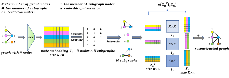
Figure 1. Overview of GNNS. Our method contains an inference model $q(Z|X,A)$ and a generative model $q(A|Z)$ for subgraph sampling. We utilize node embedding generated from GCN to perform node sampling, and extract the largest connected component from the sampled nodes as subgraphs. And then reconstructing the input graph with $Z_{n}^{T}I_{t}Z_{n}$ using the node embedding $Z_{n}$ from all subgraphs and interaction matrices $I_{t}$ of all subgraph types. Each node and corresponding nodes embedding are marked with the same color. The trapezoid represents the GCN layer. Different interaction matrix uses different shades of color to distinguish.

3. Related WorkS

Following the classification of Ribeiro (Ribeiro et al., 2021), the studies of subgraph density estimation can be classified into two categories, namely, exact estimation and approximate estimation.

3.1. Exact Methods

Exact method consists of counting the exact number of occurrences of each subgraph type. Classical methods enumerate all k-nodes subgraphs before classifying them using graph isomorphism techniques such as Nauty (McKay, 2007). Milo et al. presented the MFinder (Milo et al., 2002) technique to calculate subgraphs based on the first description of Motif. Wernicke subsequently presented a new approach, FANMOD (Wernicke, 2005), to improve MFinder so that the identical subgraph is only calculated once. Kashani et al. proposed Kavosh (Kashani et al., 2009) which enhances efficiency by locating and eliminating a certain node from all subgraphs, hence minimizing the need to cache information. The isomorphic classification step required by the conventional technique frequently costs a lot of time. To improve the calculation efficiency of specific subgraph categories, the single graph search methods were devised, such as Grochow (Grochow and Kellis, 2007), NeMo (Koskas et al., 2011) and ISMAGS (Demeyer et al., 2013). G-tries (Ribeiro and Silva, 2010b) expanded the application of the enumeration method to more generic circumstances. G-tries encapsulated the topological information shared by all subgraphs in a number of subgraphs and proposed an algorithm that stores a list of subgraphs in a specialized data structure and hence counts the number of occurrences of each subgraph in the target graph efficiently.

In addition to enumerating subgraphs explicitly, we can also count subgraphs by means of analysis. Construct a linear equation by relating the frequency of each subgraph to subgraphs with less or equal size. ORCA (Hočevar and Demšar, 2014) derives a system of equations that relate the orbit counts and solve for them using integer arithmetic. We use ORCA to compute the ground truth subgraph distribution in our experiment section 5. In addition to the analytical methods of linear algebra, there are decomposition methods that locate each subgraph by common adjacency, like ACC-MOTIF (Meira et al., 2012), PGD (Ahmed et al., 2017) and ESCAPE (Pinar et al., 2017).

3.2. Approximate Methods

Despite the high accuracy achieved by exact estimation algorithms, it is inefficient when estimating the distribution of subgraphs with a large number of nodes. With the ever-increasing graph size, approximate methods are preferable to ensure computational efficiency. Randomized enumeration methods such as (Wernicke, 2005; Ribeiro and Silva, 2010a; Paredes and Ribeiro, 2015) extends works on exact counting to perform approximation in a similar way. Another family of works is based on theories of random walk in graph: MCMC (Saha and Hasan, 2015) and Guise (Bhuiyan et al., 2012) are based on Markov chain Monte Carlo (MCMC). WRW (Han and Sethu, 2016) is also a random walk based method that can derive the concentration of subgraphs of any size. Moreover, there is a family of algorithms that relies on the idea of sampling path subgraphs (Seshadhri et al., 2013; Wang et al., 2017). Lastly, a group of algorithms is based on the idea of color coding(Alon et al., 1995; Zhao et al., 2010; Slota and Madduri, 2013).

4. Methodology

In this section, we present our method GNNS to efficiently sample sub-graphs from a large graph. GNNS can be splitted into two major phases. We first train an auto-encoder to learn an embedding for each node. Then we perform the subgraph sampling based on the learned embedding. The sampling process can be conducted in a fully-parallel manner, which guarantees GNNS as a much faster and more scalable method compared with traditional methods such as MCMC.

The learning is based on the assumptions of the generation process of the graph. Specifically, we assume that a large graph consists of a random mixture of instances, where each instance is characterized by (1) a distribution over all the nodes (2) a distribution of several types. For the sampling part, we use the relaxed Bernoulli distribution (Maddison et al., 2016) to make the sampling process differentiable and therefore ready for the back-propagation.

4.1. Inference Model

Given a graph $G(V,E)$ with $N$ nodes, we introduce an adjacency matrix $A$ to indicate the connectivity of the graph, and one-hot vector $X$ as node feature to indicate the identity of each node. We implement a graph variational auto-encoder that is composed of an inference model as in algorithm 1 and a generative model as in algorithm 2.

An inference model takes an input graph with its adjacency matrix $A$ and node feature $X$ with two-layer graph convolutional network (GCN) to generate node embedding $Z_{n}$ with a size $N\times K$. Then subgraph embedding $Z_{s}$ with a size $M\times K$, is computed with node embedding $Z_{n}$ after subgraph sampling, indicated as $q(Z_{s}|Z_{n})$. And then a subgraph is predicted from subgraph embedding, denoted as $q(Z_{t}|Z_{s})$ with a size of $M\times T$. Here $M$ is the number of sampled subgraphs, $K$ is the dimension of node embedding, $T$ is total number of subgraph types.

(1) $$q(Z|X,A)=q(Z_{t},Z_{n},Z_{s}|X,A)=q(Z_{t}|Z_{s})q(Z_{s}|Z_{n})q(Z_{n}|X,A)$$

Each node embedding ${z_{n}}_{i}$ is passed as logits into a Bernoulli distribution, and then perform node sampling $n_{i}\sim Bernoulli({z_{n}}_{i})$ with a pre-defined threshold.

(2) $$q(Z_{n}|X,A)=\prod_{i=1}^{N}q({z_{n}}_{i}|X,A)$$

In order to sample subgraphs, note that a naive node sampling may generate several unconnected components of the original graph (e.g. several disjoint subgraphs). To avoid such a problem, we sample the subgraph $G^{\prime}(V^{\prime},E^{\prime})$ from its maximal connected component based on the sampled nodes $\{n_{i}\}$ and $\{n_{j}\}$ with their connected edges $\{e_{ij}\}$. Then $M$ subgraphs could be simultaneously sampled using such a procedure. The embedding ${z_{s}}_{m}$ of the subgraph $m$ is then represented as ${z_{s}}_{m}=\sum_{i\in V^{\prime}}{z_{n}}_{i}$, which is a sum over all the embeddings of the nodes in this subgraph $G^{\prime}$. Next, the subgraph type embedding ${z_{t}}_{m}$ is predicted using a multi-layer perceptron (MLP) from a softmax distribution given by ${z_{t}}_{m}=\text{MLP}({z_{s}}_{m})$; one can then obtain the subgraph type $t=\operatorname*{arg\,max}_{t}q(t|{z_{t}}_{m})$.

4.2. Generative Model

Given an edge $e_{ij}$ between node $n_{i}$ and $n_{j}$ in subgraph $m$, a generative model $p(A|Z)$ uses the estimated node embedding $Z_{n}$ and the subgraph type $t$ predicted from subgraph embedding $Z_{s}$ to generate the edges $e_{ij}$ in the adjacency matrix $A$ of the input graph $G(V,E)$. In order to model for each subgraph type $t$, we introduce a trainable interaction matrix $I_{t}$ for each type. Given a sampled subgraph $m$, we formalize the generation of edge $p(e_{ij})=\sigma({z_{n}}_{i}^{T}I_{t}{z_{n}}_{j})$ of $E^{\prime}$ using the learned node embedding $z_{n}$ and predicted subgraph type $t$. Given $M$ subgraphs with all $T$ types are sampled from an input graph at the same time, we represent the probability of reconstructed edge by the following summation over all types and subgraphs

(3) $$p(A|Z)=\sum_{i=1}^{N}\sum_{j=1}^{N}\sum_{t=1}^{T}\sum_{m=1}^{M}\sigma({z_{n}}_{i}^{T}I_{t}{z_{n}}_{j}),i\in m,j\in m$$

4.3. Objective Function

We optimize our inference model $q(Z|X,A)$ and generative model $p(A|Z)$ using the evidence lower bound (ELBO), which maximizes the data likelihood and minimizes the KL divergence between the approximated posterior distribution and prior distribution. We assume a non-informative prior distribution $p(Z)$. The objective function is as follows

(4) $$\mathcal{L}=\mathbb{E}_{q}(Z|X,A)[\text{log}p(A|Z)]-\text{KL}(q(Z|X,A)||p(Z))$$

1:  Compute node embedding $Z_{n}=GNN(X,A)$ from graph $G(V,E)$

2:  for each node $i$ do

3:     Sample node using $n_{i}\sim Bernoulli({z_{n}}_{i})$

4:  end for

5:  Extract the largest connected component from the set of sampled nodes ${n_{i}}$ as a sampled subgraph $G^{\prime}(V^{\prime},E^{\prime})\subseteq G(V,E)$

6:  for each subgraph $m$ do

7:     Compute subgraph embedding ${z_{s}}_{m}=\sum_{i\in m}{z_{n}}_{i}$

8:     Compute subgraph type embedding ${z_{t}}_{m}=\text{MLP}({z_{s}}_{m})$

9:     Predict subgraph type $t=\operatorname*{arg\,max}_{t}q(t|{z_{t}}_{m})$

10:  end for

Algorithm 1 Inference model $q(Z|X,A)$ of GNNS

1:  for each subgraph type $t$ do

2:     for each subgraph $m$ do

3:        for each node pair $(i,j)$ inside subgraph $m$ do

4:           generate edge $p(e_{ij})=\sigma({z_{n}}_{i}^{T}I_{t}{z_{n}}_{j})$

5:        end for

6:     end for

7:  end for

8:  sum $p(e_{ij}),i\in m,j\in m$ over all $M$ subgraphs and $T$ subgraph types to reconstruct the adjacency matrix $A$ from graph $G(V,E)$

Algorithm 2 Generative model $p(A|Z)$ of GNNS

5. Experiments

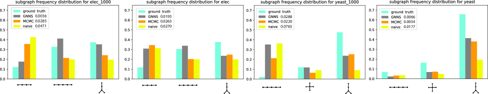
Figure 2. Approximated distributions of subgraph types with top 3 frequencies for each method. We evaluate the accuracy of the sampled distribution from our proposed method GNNS compared with MCMC (Saha and Hasan, 2015), naive sampling and ground truth (Hočevar and Demšar, 2014). Mean squared error (MSE) of the 3 most representative graphs on both Yeast and Elec dataset is provided.

We evaluate GNNS on both real world graphs and simulated graphs for subgraph types that have 4-nodes and 5-nodes. All experiments are implemented on NVIDIA GeForce RTX 2080 Ti. All training parameters are updated by the Adam Optimizer with a learning rate of $1\times 10^{-3}$. For the parameters of the model architecture, we choose the pre-defined parameters M (number of sampled subgraphs) = 1024, K (dimension of node embedding) =256 and T (total number of subgraph types) = 16. Note these parameters are based purely on empirical experience. Since most graphs have a long-tailed density distribution, underestimating subgraph types would not be an issue. We compare the result with the MHRW version of the MCMC sampling method  (Saha and Hasan, 2015) where we used the authors’ published code. For completeness, we also introduce a naive sampling method that enables estimation by uniformly drawing nodes from graphs to form induced subgraphs. We evaluate the methods’ performance from 2 aspects: accuracy and runtime. To compute the accuracy, we obtain the ground truth subgraph frequency distribution from the exact counting method: ORCA (Hočevar and Demšar, 2014). We then use the mean squared error (MSE) between the models’ estimated frequency distribution and the ground truth distribution to assess the accuracy.

5.1. Dataset

For experiments, we select one biological network —the Yeast transcription network (with 688 nodes and 1046 edges) and one network from engineering —the Electrical network (with 252 nodes and 397 edges) (Kashani et al., 2009).

For network pre-processing, we apply the same technique as in the MCMC method: we check for undirected graphs and remove duplicate edges in the network. After that, we randomly generated 1000 random graphs following the same degree distribution as each network. We then do a Train-Valid-Test split on the 1000 random graphs dataset. The split ratio is 8:1:1. The goal here is to accurately predict the subgraph frequency distribution the test set based on the model trained on the training set. Note the training set and test set share a same degree of distribution, which means the model should be able to generalize to the test set.

5.2. Accuracy Comparison

We use the mean squared error (MSE) between the ground truth distribution and the estimated distribution as the metric of estimation performance. For convenience, we combine the subgraphs with 4 and 5 nodes when computing the subgraph frequency distribution (i.e., the denominator of each term in the distribution vector in Def 2.6 is now the sum of the frequency of all 4-subgraph types and 5-subgraph types.) Table 1 shows that our methods outperform MCMC (and naive sampling) in most circumstances. In Figure 2, we visualize the approximated distribution of each method as a bar chart and demonstrate three subgraph types with the highest frequency.

Dataset	GNNS	Naive Sampling	MCMC
Scale	$1\mathrm{e}{-3}$	$1\mathrm{e}{-3}$	$1\mathrm{e}{-3}$
Elec	2.32	3.64	3.30
Yeast	6.55	17.20	7.85
Elec1000	0.73	3.98	3.50
Yeast1000	8.83	13.30	5.32

Table 1. Sampling quality comparsion (MSE). Elec and yeast stand for the single original graphs. Elec1000 and Yeast1000 stand for the average of 1000 random graphs sampled from Elec and Yeast, respectively.

5.3. Runtime Comparison

We use the total running time on the 1000 random graphs in the three approaches for runtime comparison. Table 2 shows the results. GNNS tallied the forward and sampling procedure, whereas Naive Sampling and MCMC only tallied the sampling time. GNNS is clearly superior to MCMC in terms of time, which significantly enhances the computational performance. The acceleration of deep learning demonstrates the significant potential of our model for estimating the frequency distribution of subgraphs.

Dataset	GNNS	Naive Sampling	MCMC
Scale	$1\mathrm{e}{-2}$	$1\mathrm{e}{-2}$	$1\mathrm{e}{-2}$
Elec1000	12.01	0.81	58400
Yeast1000	24.45	0.86	257100

Table 2. Sampling time comparison (in seconds). Elec1000 and Yeast1000 stand for the running time on the 1000 random graphs sampled from Elec and Yeast, respectively.

6. Conclusion

In this work, we propose GNNS, a learning-based representation framework, which utilizes graph neural networks to learn hierarchical embeddings on the node, subgraph, and type levels. We perform subgraph sampling in a highly scalable and parallel way. Experiments show that our proposed framework achieves a comparable accuracy and a significant speed-up compared to MCMC-sampling with three orders of magnitude. We also think of a lot of interesting future directions, e.g. motif search, that could benefit from our proposed graph neural network based sampling.

References

- (1)
- Ahmed et al. (2017) Nesreen K Ahmed, Jennifer Neville, Ryan A Rossi, Nick G Duffield, and Theodore L Willke. 2017. Graphlet decomposition: Framework, algorithms, and applications. Knowledge and Information Systems 50, 3 (2017), 689–722.
- Alon et al. (1995) Noga Alon, Raphael Yuster, and Uri Zwick. 1995. Color-coding. Journal of the ACM (JACM) 42, 4 (1995), 844–856.
- Bhuiyan et al. (2012) Mansurul A Bhuiyan, Mahmudur Rahman, Mahmuda Rahman, and Mohammad Al Hasan. 2012. Guise: Uniform sampling of graphlets for large graph analysis. In 2012 IEEE 12th International Conference on Data Mining. IEEE, 91–100.
- Costa et al. (2011) Luciano da Fontoura Costa, Osvaldo N Oliveira Jr, Gonzalo Travieso, Francisco Aparecido Rodrigues, Paulino Ribeiro Villas Boas, Lucas Antiqueira, Matheus Palhares Viana, and Luis Enrique Correa Rocha. 2011. Analyzing and modeling real-world phenomena with complex networks: a survey of applications. Advances in Physics 60, 3 (2011), 329–412.
- Demeyer et al. (2013) Sofie Demeyer, Tom Michoel, Jan Fostier, Pieter Audenaert, Mario Pickavet, and Piet Demeester. 2013. The index-based subgraph matching algorithm (ISMA): fast subgraph enumeration in large networks using optimized search trees. PloS one 8, 4 (2013), e61183.
- Grochow and Kellis (2007) Joshua A Grochow and Manolis Kellis. 2007. Network motif discovery using subgraph enumeration and symmetry-breaking. In Annual International Conference on Research in Computational Molecular Biology. Springer, 92–106.
- Han and Sethu (2016) Guyue Han and Harish Sethu. 2016. Waddling random walk: Fast and accurate mining of motif statistics in large graphs. In 2016 IEEE 16th International Conference on Data Mining (ICDM). IEEE, 181–190.
- Hočevar and Demšar (2014) Tomaž Hočevar and Janez Demšar. 2014. A combinatorial approach to graphlet counting. Bioinformatics 30, 4 (2014), 559–565.
- Itzkovitz and Alon (2005) Shalev Itzkovitz and Uri Alon. 2005. Subgraphs and network motifs in geometric networks. Physical Review E 71, 2 (2005), 026117.
- Juszczyszyn et al. (2008) Krzysztof Juszczyszyn, Przemysław Kazienko, and Katarzyna Musiał. 2008. Local topology of social network based on motif analysis. In International Conference on Knowledge-Based and Intelligent Information and Engineering Systems. Springer, 97–105.
- Kashani et al. (2009) Zahra Razaghi Moghadam Kashani, Hayedeh Ahrabian, Elahe Elahi, Abbas Nowzari-Dalini, Elnaz Saberi Ansari, Sahar Asadi, Shahin Mohammadi, Falk Schreiber, and Ali Masoudi-Nejad. 2009. Kavosh: a new algorithm for finding network motifs. BMC Bioinformatics 10, 1 (2009), 318. https://doi.org/10.1186/1471-2105-10-318
- Koskas et al. (2011) Michel Koskas, Gilles Grasseau, Etienne Birmelé, Sophie Schbath, and Stéphane Robin. 2011. NeMo: Fast count of network motifs. Book of Abstracts for Journées Ouvertes Biologie Informatique Mathématiques (JOBIM) 2011 (2011), 53–60.
- Maddison et al. (2016) Chris J Maddison, Andriy Mnih, and Yee Whye Teh. 2016. The concrete distribution: A continuous relaxation of discrete random variables. arXiv preprint arXiv:1611.00712 (2016).
- McKay (2007) Brendan D McKay. 2007. Nauty user’s guide (version 2.4). Computer Science Dept., Australian National University (2007), 225–239.
- Meira et al. (2012) Luis AA Meira, Vinicius R Maximo, Alvaro L Fazenda, and Arlindo F da Conceicao. 2012. Accelerated motif detection using combinatorial techniques. In 2012 Eighth International Conference on Signal Image Technology and Internet Based Systems. IEEE, 744–753.
- Melckenbeeck et al. (2018) Ine Melckenbeeck, Pieter Audenaert, Didier Colle, and Mario Pickavet. 2018. Efficiently counting all orbits of graphlets of any order in a graph using autogenerated equations. Bioinformatics 34, 8 (2018), 1372–1380.
- Milo et al. (2002) Ron Milo, Shai Shen-Orr, Shalev Itzkovitz, Nadav Kashtan, Dmitri Chklovskii, and Uri Alon. 2002. Network motifs: simple building blocks of complex networks. Science 298, 5594 (2002), 824–827.
- Paredes and Ribeiro (2015) Pedro Paredes and Pedro Ribeiro. 2015. Rand-fase: fast approximate subgraph census. Social Network Analysis and Mining 5, 1 (2015), 1–18.
- Pinar et al. (2017) Ali Pinar, C Seshadhri, and Vaidyanathan Vishal. 2017. Escape: Efficiently counting all 5-vertex subgraphs. In Proceedings of the 26th international conference on world wide web. 1431–1440.
- Ribeiro et al. (2021) Pedro Ribeiro, Pedro Paredes, Miguel EP Silva, David Aparicio, and Fernando Silva. 2021. A survey on subgraph counting: concepts, algorithms, and applications to network motifs and graphlets. ACM Computing Surveys (CSUR) 54, 2 (2021), 1–36.
- Ribeiro and Silva (2010a) Pedro Ribeiro and Fernando Silva. 2010a. Efficient subgraph frequency estimation with g-tries. In International Workshop on Algorithms in Bioinformatics. Springer, 238–249.
- Ribeiro and Silva (2010b) Pedro Ribeiro and Fernando Silva. 2010b. G-tries: an efficient data structure for discovering network motifs. In Proceedings of the 2010 ACM symposium on applied computing. 1559–1566.
- Saha and Hasan (2015) Tanay Kumar Saha and Mohammad Al Hasan. 2015. Finding network motifs using MCMC sampling. In Complex Networks VI. Springer, 13–24.
- Seshadhri et al. (2013) Comandur Seshadhri, Ali Pinar, and Tamara G Kolda. 2013. Triadic measures on graphs: The power of wedge sampling. In Proceedings of the 2013 SIAM international conference on data mining. SIAM, 10–18.
- Slota and Madduri (2013) George M Slota and Kamesh Madduri. 2013. Fast approximate subgraph counting and enumeration. In 2013 42nd International Conference on Parallel Processing. IEEE, 210–219.
- Solé and Munteanu (2004) Ricard V Solé and Andreea Munteanu. 2004. The large-scale organization of chemical reaction networks in astrophysics. EPL (Europhysics Letters) 68, 2 (2004), 170.
- Wang et al. (2017) Pinghui Wang, Junzhou Zhao, Xiangliang Zhang, Zhenguo Li, Jiefeng Cheng, John CS Lui, Don Towsley, Jing Tao, and Xiaohong Guan. 2017. MOSS-5: A fast method of approximating counts of 5-node graphlets in large graphs. IEEE Transactions on Knowledge and Data Engineering 30, 1 (2017), 73–86.
- Wernicke (2005) Sebastian Wernicke. 2005. A faster algorithm for detecting network motifs. In International Workshop on Algorithms in Bioinformatics. Springer, 165–177.
- Zhao et al. (2010) Zhao Zhao, Maleq Khan, VS Anil Kumar, and Madhav V Marathe. 2010. Subgraph enumeration in large social contact networks using parallel color coding and streaming. In 2010 39th International Conference on Parallel Processing. IEEE, 594–603.