Stochastic Optimal and Time-Optimal Control Studies for Additional Food provided prey-predator Systems involving Holling Type-III Functional Response

Abstract

This paper consists of a detailed and novel stochastic optimal control analysis of a coupled non-linear dynamical system. The state equations are modeled as additional food provided prey-predator system with Holling Type-III functional response for predator and intra-specific competition among predators. We firstly discuss the optimal control problem as a Lagrangian problem with a linear quadratic control. Secondly we consider an optimal control problem in the time-optimal control setting. Stochastic maximum principle is used for establishing the existence of optimal controls for both these problems. Numerical simulations are performed based on stochastic forward-backward sweep methods for realizing the theoretical findings. The results obtained in these optimal control problems are discussed in the context of biological conservation and pest management.

1 Introduction

Millions of species coexist in this universe where the survival of each species is meticulously woven with respect to other species. The survival of one species(say, predator) is dependent on the existence of other species(say, prey). The very first mathematical models of such interactive species were given by Alfred J. Lotka [1] and Vito Volterra [2] in 1925. In the last century, various mathematical models were proposed and their behaviours were studied.

One of the primary component in defining the predator-prey dynamics is the functional response. The functional response is the rate at which each predator captures prey [3]. A type III functional response is a sigmoidal response [4] that has predators foraging inefficiently at low prey densities. The Holling type III functional response is displayed by many organisms in nature [5, 6, 7, 8]. Some studies involving additional food-provided prey-predator systems with Holling type III and type IV functional responses can be found in [9, 10]. Recently, the authors in [11, 12, 13] have studied controllability of additional food systems with respect to quality and quantity of additional food as control variables for type III and type IV systems.

Also, in real world situations, some of the the parameters involved in the model always fluctuate around some average value due to continuous variation in the environment. A large number of researchers introduced a stochastic environmental variation using the Brownian motion into parameters in the deterministic model to construct a stochastic model. The authors in [14] proved that a stochastic predator-prey model with a protection zone has a unique stationary distribution which is ergodic. In [15] the authors obtained stochastic permenace for a stochastic predator-prey system with Holling-type III functional response. The work [16] deals with a a Holling-type II stochastic predator-prey model with additional food that has an ergodic stationary distribution. The authors in [17] studied the deterministic and stochastic dynamics of a modified Leslie-Gower prey-predator system with a simplified Holling-type IV scheme. The work [18] deals with the survival and ergodicity of a stochastic Holling-type III predator-prey model with markovian switching in an impulsive polluted environment. In the recent times, optimal control theory is being applied on various stochastic models in order to achieve optimal control values which minimizes the cost. Also to our knowledge very limited research exists on optimal control theory for additional food provided stochastic predator-prey systems involving different functional responses.

Motivated by the above discussions, in this paper, we study two optimal control problems on an additional food provided prey-predator system with Holling type-III functional response for predator. This system is a coupled non-linear dynamical system. The first optimal control problem is a Lagrange problem. This has applications for biological conservation of species where we find the optimal quality and quantity of additional food to be provided to predator in order to maximize the populations of predator and prey [19, 20, 21]. The second optimal control problem is a special kind of optimal control problem, known as time-optimal control problem, where we determine the optimal additional food to be provided to system in order to reach the final state in minimum time. This has several applications to pest management [13, 12, 11, 22, 23].

The rest of the paper is organised as follows. In section 2, we formulate the stochastic model for additonal food provided system involving Holling type III response. Section 3 deals with the discussion on corresponding linear quadratic optimal control problems with applications to biological conservation with reference to quality and quantity of additional food as stochastic control variables. Later in section 4 we deal with the time optimal control problems for these systems with applications to both biological conservation and pest management. Numerical simulations are also done to validate the theoretical findings in sections 3-4. Finally in section 5, we do the discussions and conclusions.

2 Stochastic Model Formulation

In this work we consider the following deterministic prey-predator model with Holling type-III functional response and additional food for predator given by:

$$\begin{split}\frac{\mathrm{d}N(t)}{\mathrm{d}t}&=rN(t)\Bigg{(}1-\frac{N(t)}{K}\Bigg{)}-\frac{cN^{2}(t)P(t)}{a^{2}+N^{2}(t)+\alpha\eta A^{2}}\\ \frac{\mathrm{d}P(t)}{\mathrm{d}t}&=g\Bigg{(}\frac{N^{2}(t)+\eta A^{2}}{a^{2}+N^{2}(t)+\alpha\eta A^{2}}\Bigg{)}-mP(t)-dP^{2}(t)\end{split}$$ (1)

The biological descriptions of the various parameters involved in the system (1) are described in Table 1.

The basic analysis for the model (1) can be done in similar lines to analysis done in [24].

To reduce the complexity in the analysis, we now reduce the number of parameters in the model (1) by introducing the transformations $N=ax,P=\frac{ay}{c}$. Then the system (1) gets transformed to:

$$\begin{split}\frac{\mathrm{d}x(t)}{\mathrm{d}t}&=rx(t)\Bigg{(}1-\frac{x(t)}{\gamma}\Bigg{)}-\frac{x^{2}(t)y(t)}{1+x^{2}(t)+\alpha\xi}\\ \frac{\mathrm{d}y(t)}{\mathrm{d}t}&=gy(t)\Bigg{(}\frac{x^{2}(t)+\xi}{1+x^{2}(t)+\alpha\xi}\Bigg{)}-my(t)-\delta y^{2}(t)\end{split}$$ (2)

where $\gamma=\frac{K}{a},\xi=\eta(\frac{A}{a})^{2},\delta=\frac{da}{c}$.

As in [14, 15], we now suppose that the intrinsic growth rate of prey and the death rate of predator are mainly affected by environmental noise such that

$$r\rightarrow r+\sigma_{1}dW_{1}(t),m\rightarrow m+\sigma_{2}dW_{2}(t)$$

where $W_{i}(t)(i=1,2)$ are the mutually independent standard Brownian motions with $W_{i}(0)=0$ and $\sigma_{1}$ and $\sigma_{2}$ are positive constants and they represent the intensities of the white noise. Hence, the system (2) wiht the environmental noise for parameters $r$ and $m$ and the Holling-type III predator functional response now becomes

$$\begin{split}dx&=\left[rx(t)\Bigg{(}1-\frac{x(t)}{\gamma}\Bigg{)}-\frac{x^{2}(t)y(t)}{1+x^{2}(t)+\alpha\xi}\right]dt+\sigma_{1}x(t)dW_{1}(t)\\ dy&=\left[gy(t)\Bigg{(}\frac{x^{2}(t)+\xi}{1+x^{2}(t)+\alpha\xi}\Bigg{)}-my(t)-\delta y^{2}(t)\right]dt+\sigma_{2}y(t)dW_{2}(t)\end{split}$$ (3)

The biological descriptions of the various parameters involved in the systems (2) and (3) are described in Table 1.

Table 1: Description of variables and parameters present in the systems (1), (2), (3)

Parameter	Definition	Dimension
T	Time	time
N	Prey density	biomass
P	Predator density	biomass
A	Additional food	biomass
r	Prey intrinsic growth rate	time-1
K	Prey carrying capacity	biomass
c	Rate of predation	time-1
a	Half Saturation value of the predators	biomass
g	Conversion efficiancy	time-1
m	death rate of predators in absence of prey	time-1
d	Predator Intra-specific competition	biomass-1 time-1
$\alpha$	quality of additional food	Dimensionless
$\xi$	quantity of additional food	biomass2

Existence of global positive solution: For any initial value $(x_{0},y_{0})\in\mathcal{R}_{+}^{2}$ there exists a unique solution $(x(t),y(t))$ of system (3) on $t\geq 0$ and the solution will remain in $\mathcal{R}_{+}^{2}$ with probability 1.

The above theorem for existence of solutions of (3) can be proved in similar lines to the proof in [15] using the Lyapunov method.

3 Stochastic Optimal Control Problem

In this section we theoretically establish the existence of optimal control for the system (3) with both quality and quantity of additional food as stochastic controls respectively. We also numerically simulate and depict the same with applications to biological conservation.

We now establish the existence of stochastic optimal control using the following stochastic maximum principle [25].

Stochastic Maximum Principle:

Theorem 1

For a stochastic controlled system

$$\begin{cases}dX(t)=b(t,X(t),u(t))dt+\sigma(t,X(t),u(t))dW(t),t\in[0,T],\\ X(0)=X_{0},\end{cases}$$ (4)

with the cost functional

$$J(u(t))=E\Big{[}\int_{0}^{T}f(t,X(t),u(t))dt+h(X(T))\Big{]},$$ (5)

with $b(t,X(t),u(t)):[0,T]\times\mathcal{R}^{n}\times U\rightarrow\mathcal{R}^{n},\sigma(t,X(t),u(t)):[0,T]\times\mathcal{R}^{n}\times U\rightarrow\mathcal{R}^{n\times m}$ and for $T$ denoting the terminal time, $f(t,X(t),u(t))$ the running cost and $h(X(T))$ the terminal cost with $(\bar{u},\bar{X})=(\bar{u},\bar{X}(\bar{u},.))$ as the optimal control and the corresponding optimal state trajectories

then there exist pairs of processes $(p(.),q(.))\in L_{F}^{2}(0,T;\mathcal{R}^{n})\times(L_{F}^{2}(0,T;\mathcal{R}^{n}))^{m}$ satisfying the first order adjoint equations

$$\begin{cases}dp(t)&=-\Big{[}b_{X}(t,\bar{X}(t),\bar{u}(t))^{T}p(t)+\sum_{n=1}^{m}\sigma_{X}^{j}(t,\bar{X}(t),\bar{u}(t))^{T}q_{j}(t)-f_{x}(t,\bar{X}(t),\bar{u}(t))\Big{]}dt+q(t)dW(t),\\ p(T)&=-h_{X}(\bar{X}(T)),\end{cases}$$ (6)

and the Variational Inequalitiy (Hamiltonian Maximization Condition)

$$\mathcal{H}(t,\bar{X}(t),\bar{u}(t))=\max_{u\in U}H(t,\bar{X}(t),u(t),p,q),$$ (7)

with the Hamiltonian functional given by

$$H(t,X,u,p,q)=\left\langle p,b\right\rangle+tr[q^{T}\sigma]-f(t,X(t),u(t))$$ (8)

3.1 Quality of additional food as control

In this section we wish to achieve biological conservation of maximizing prey and predator population for the system (3) with quality of additional food as a control variable with minimum supply of the food.

To attain this we consider the following objective functional with the state equations (3)

$$J(u)=E\Bigg{[}\int_{0}^{T}\Bigg{(}-A_{1}x(t)-A_{2}y(t)+A_{3}\frac{\alpha^{2}(t)}{2}\Bigg{)}dt\Bigg{]}$$ (9)

where $A_{1},A_{2},A_{3}$ are positive constants.

Here our goal is to find an optimal control $\alpha^{*}$ such that $J(\alpha^{*})\leq J(\alpha),\forall\alpha(t)\in U$ where $U$ is an admissible control set defined by $U=\{\alpha(t)|0\leq\alpha(t)\leq\alpha_{max}\forall t\in(0,t_{f}]\}$ where $\alpha_{max}\in\mathcal{R}^{+}$.

Now to find the optimal control $\alpha^{*}$ using the stochastic maximum principle we find the similars for the system (3) with (4). Comparing the stochastic system (3) with (4), the vectors $X,b,\sigma$ can be seen as

$$X(t)=\begin{pmatrix}x(t)\\ y(t)\end{pmatrix},\ b(t,X(t),u(t))=\begin{pmatrix}b_{1}(t)\\ b_{2}(t)\end{pmatrix}=\begin{pmatrix}rx(t)(1-\frac{x(t)}{\gamma})-\frac{x^{2}(t)y(t)}{1+x^{2}(t)+\alpha\xi}\\ gy(t)(\frac{x^{2}(t)+\xi}{1+x^{2}(t)+\alpha\xi})-my(t)-\delta y^{2}(t)\end{pmatrix},$$

$$\sigma(t,X(t),u(t))=\begin{pmatrix}\sigma_{1}x(t)&0\\ 0&\sigma_{2}y(t)\end{pmatrix},\ dW(t)=\begin{pmatrix}dW_{1}(t)\\ dW_{2}(t)\end{pmatrix}$$

We also note that

$$b_{X}=\begin{pmatrix}\frac{\partial b_{1}}{\partial x}&\frac{\partial b_{1}}{\partial y}\\ \frac{\partial b_{2}}{\partial x}&\frac{\partial b_{2}}{\partial y}\end{pmatrix}=\begin{pmatrix}r(1-\frac{2x}{\gamma})-\frac{2xy(1+\alpha\xi)}{(1+x^{2}+\alpha\xi)^{2}}&\frac{-x^{2}}{1+x^{2}+\alpha\xi}\\ \frac{2gxy(1+(\alpha-1)\xi)}{(1+x^{2}+\alpha\xi)^{2}}&g(\frac{x^{2}+\xi}{1+x^{2}+\alpha\xi})-m-2\delta y\end{pmatrix}$$ (10)

$$\begin{split}\sigma^{1}=\begin{pmatrix}\sigma_{1}x\\ 0\end{pmatrix}\Rightarrow\sigma_{X}^{1}=\begin{pmatrix}\frac{\partial}{\partial x}(\sigma_{1}x)&\frac{\partial}{\partial y}(\sigma_{1}x)\\ \frac{\partial}{\partial x}(0)&\frac{\partial}{\partial y}(0)\end{pmatrix}=\begin{pmatrix}\sigma_{1}&0\\ 0&0\end{pmatrix}\\ \sigma^{2}=\begin{pmatrix}0\\ \sigma_{2}y\end{pmatrix}\Rightarrow\sigma_{X}^{2}=\begin{pmatrix}\frac{\partial}{\partial x}(0)&\frac{\partial}{\partial y}(0)\\ \frac{\partial}{\partial x}(\sigma_{2}y)&\frac{\partial}{\partial y}(\sigma_{2}y)\end{pmatrix}=\begin{pmatrix}0&0\\ 0&\sigma_{2}\end{pmatrix}\\ \end{split}$$ (11)

As the diffusion term $\sigma$ in (11) is independent of the control, the solution of the second-order adjoint equations will not be helpful in calculating the optimal control values.

Now comparing the cost functional (9) with (5), we see that

$f(t,X(t),u(t))=-A_{1}x(t)-A_{2}y(t)+A_{3}\frac{\alpha^{2}(t)}{2}$ and $h(X(T))=0$.

Hence from the stochastic maximum principle, there exist stochastic processes

$(p(.),q(.))\in L_{F}^{2}(0,T;\mathcal{R}^{n})\times(L_{F}^{2}(0,T;\mathcal{R}^{n}))^{m},\ p(t)=\begin{pmatrix}p_{1}(t)\\ p_{2}(t)\end{pmatrix},\ q(t)=\begin{pmatrix}q_{1}(t)&q_{3}(t)\\ q_{2}(t)&q_{4}(t)\end{pmatrix}\ni$

$$\begin{split}\begin{pmatrix}dp_{1}(t)\\ dp_{2}(t)\end{pmatrix}&=-\Bigg{[}\begin{pmatrix}\frac{\partial b_{1}}{\partial x}&\frac{\partial b_{2}}{\partial x}\\ \frac{\partial b_{1}}{\partial y}&\frac{\partial b_{2}}{\partial y}\end{pmatrix}\begin{pmatrix}p_{1}(t)\\ p_{2}(t)\end{pmatrix}+\sigma_{X}^{1}(t,\bar{X}(t),\bar{u}(t))^{T}q_{1}(t)+\sigma_{X}^{2}(t,\bar{X}(t),\bar{u}(t))^{T}q_{2}(t)-\begin{pmatrix}\frac{\partial f}{\partial x}\\ \frac{\partial f}{\partial y}\end{pmatrix}\Bigg{]}dt\\ &+\begin{pmatrix}q_{1}(t)&q_{3}(t)\\ q_{2}(t)&q_{4}(t)\end{pmatrix}\begin{pmatrix}dW_{1}(t)\\ dW_{2}(t)\end{pmatrix}\\ p_{1}(T)&=0,\ p_{2}(T)=0.\end{split}$$

Substituting $\frac{\partial f}{\partial x}=-A_{1},\frac{\partial f}{\partial y}=-A_{2}$ and the values of $b_{X},\sigma_{X}^{1},\sigma_{X}^{2}$ from (10), (11), we see that the adjoint equations for the optimal control $\alpha^{*}$ are given as:

$$\begin{split}dp_{1}(t)&=-\Bigg{[}\frac{\partial b_{1}}{\partial x}p_{1}(t)+\frac{\partial b_{2}}{\partial x}p_{2}(t)+\sigma_{1}q_{1}+A_{1}\Bigg{]}dt+q_{1}(t)dW_{1}(t)+q_{3}(t)dW_{2}(t)\\ dp_{2}(t)&=-\Bigg{[}\frac{\partial b_{1}}{\partial y}p_{1}(t)+\frac{\partial b_{2}}{\partial y}p_{2}(t)+\sigma_{2}q_{4}+A_{2}\Bigg{]}dt+q_{2}(t)dW_{1}(t)+q_{4}(t)dW_{2}(t)\\ p_{1}(T)&=0,\ p_{2}(T)=0\end{split}$$

On further simplification we see that

$$\begin{split}dp_{1}(t)&=-\Bigg{[}\Big{(}r(1-\frac{2x}{\gamma})-\frac{2xy(1+\alpha\xi)}{(1+x^{2}+\alpha\xi)^{2}}\Big{)}p_{1}(t)+\frac{2gxy(1+(\alpha-1)\xi)}{(1+x^{2}+\alpha\xi)^{2}}p_{2}(t)+\sigma_{1}q_{1}+A_{1}\Bigg{]}dt\\ &+q_{1}(t)dW_{1}(t)+q_{3}(t)dW_{2}(t)\\ dp_{2}(t)&=-\Bigg{[}\frac{-x^{2}}{1+x^{2}+\alpha\xi}p_{1}(t)+\Big{(}g(\frac{x^{2}+\xi}{1+x^{2}+\alpha\xi})-m-2\delta y\Big{)}p_{2}(t)+\sigma_{2}q_{4}+A_{2}\Bigg{]}dt\\ &+q_{2}(t)dW_{1}(t)+q_{4}(t)dW_{2}(t)\\ p_{1}(T)&=0,\ p_{2}(T)=0.\end{split}$$ (12)

The solutions of the above equations (12) gives $(p_{1}(t),p_{2}(t))$, which are the co-state vectors.

Now from (8), we see that the Hamiltonian for the system (3) is given by:

$$\begin{split}H(t,X,u,p,q)&=\left\langle p,b\right\rangle+tr[q^{T}\sigma]+A_{1}x(t)+A_{2}y(t)-A_{3}\frac{\alpha^{2}(t)}{2}\\ &=\begin{pmatrix}p_{1}(t)&p_{2}(t)\end{pmatrix}\begin{pmatrix}b_{1}(t)\\ b_{2}(t)\end{pmatrix}+tr\Bigg{[}\begin{pmatrix}q_{1}(t)&q_{2}(t)\\ q_{3}(t)&q_{4}(t)\end{pmatrix}\begin{pmatrix}\sigma_{1}x&0\\ 0&\sigma_{2}y\end{pmatrix}\Bigg{]}+A_{1}x(t)+A_{2}y(t)-A_{3}\frac{\alpha^{2}(t)}{2}\\ &=p_{1}(t)b_{1}+p_{2}(t)b_{2}+q_{1}\sigma_{1}x+q_{4}\sigma_{2}y+A_{1}x(t)+A_{2}y(t)-A_{3}\frac{\alpha^{2}(t)}{2}\\ &=\Big{(}rx(t)(1-\frac{x(t)}{\gamma})-\frac{x^{2}(t)y(t)}{1+x^{2}(t)+\alpha\xi}\Big{)}p_{1}(t)+\Big{(}gy(t)(\frac{x^{2}(t)+\xi}{1+x^{2}(t)+\alpha\xi})-my(t)-\delta y^{2}(t)\Big{)}p_{2}(t)\\ &+q_{1}\sigma_{1}x+q_{4}\sigma_{2}y+A_{1}x(t)+A_{2}y(t)-A_{3}\frac{\alpha^{2}(t)}{2}\\ \end{split}$$

Now from the Hamiltonian maximization condition (7), we have

$$\begin{split}\mathcal{H}(t,\bar{X}(t),\bar{\alpha}(t))&=\max_{\alpha\in U}H(t,\bar{X}(t),\alpha(t))\\ \implies\frac{\partial H}{\partial\alpha}&=0\\ \end{split}$$

$$\begin{split}\implies&\frac{\partial}{\partial\alpha}\Big{(}rx(t)(1-\frac{x(t)}{\gamma})-\frac{x^{2}(t)y(t)}{1+x^{2}(t)+\alpha\xi}\Big{)}p_{1}+\frac{\partial}{\partial\alpha}\Big{(}gy(t)(\frac{x^{2}(t)+\xi}{1+x^{2}(t)+\alpha\xi})-my(t)-\delta y^{2}(t)\Big{)}p_{2}(t)\\ +&\frac{\partial}{\partial\alpha}(q_{1}\sigma_{1}x+q_{4}\sigma_{2}y+A_{1}x(t)+A_{2}y(t)-A_{3}\frac{\alpha^{2}(t)}{2})=0\\ \implies&\frac{\xi x^{2}yp_{1}}{(1+x^{2}+\alpha\xi)^{2}}-\frac{\xi gyp_{2}(x^{2}+\xi)}{(1+x^{2}+\alpha\xi)^{2}}-A_{3}\alpha=0\\ &\ \\ \implies&(A_{3}\xi^{2})\alpha^{3}+(2A_{3}\xi(1+x^{2}))\alpha^{2}+(A_{3}(1+x^{2})^{2})\alpha+(\xi gyp_{2}(x^{2}+\xi)-\xi x^{2}yp_{1})=0.\end{split}$$

Now from Descartes’ rule of signs, we see that the above cubic equation admits a positive $\alpha$ only if $gp_{2}(x^{2}+\xi)-x^{2}p_{1}<0$.

On solving the above cubic equation, we see that the optimal quality control is given by

$$\alpha^{*}=\frac{(1+x^{2}-c_{0}\xi)^{2}}{3c_{0}\xi^{2}},$$ (13)

$$\begin{split}\text{where, }c_{0}&=\bigg{(}\frac{-10(1+x^{2})^{3}}{\xi^{3}}+\frac{27yc_{1}}{2A_{3}\xi}+\frac{1}{2}\sqrt{\frac{-108c_{1}y(1+x^{2})^{2}}{A_{3}\xi^{4}}+\frac{729y^{2}c_{1}^{2}}{A_{3}^{2}\xi^{2}}}\bigg{)}^{\frac{1}{3}}\\ \text{and }c_{1}&=gp_{2}(x^{2}+\xi)-x^{2}y\end{split}$$

3.2 Quantity of additional food as control

In this section we wish to achieve biological conservation of maximizing prey and predator population for the system (3) with quantity of additional food as a control variable with minimum supply of the food.

To attain this we consider the following objective functional with the state equations (3)

$$J(u)=E\Bigg{[}\int_{0}^{T}\Bigg{(}-A_{1}x(t)-A_{2}y(t)+A_{3}\frac{\xi^{2}(t)}{2}\Bigg{)}dt\Bigg{]}$$ (14)

where $A_{1},A_{2},A_{3}$ are positive constants.

Here our goal is to find an optimal control $\xi^{*}$ such that $J(\xi^{*})\leq J(\xi),\forall\xi(t)\in U$ where $U$ is an admissible control set defined by $U=\{\xi(t)|0\leq\xi(t)\leq\xi_{max}\forall t\in(0,t_{f}]\}$ where $\xi_{max}\in\mathcal{R}^{+}$.

Now comparing the cost functional (14) with (5), we see that

$f(t,X(t),u(t))=-A_{1}x(t)-A_{2}y(t)+A_{3}\frac{\xi^{2}(t)}{2}$ and $h(X(T))=0$.

Since $\frac{\partial f}{\partial x}$ and $\frac{\partial f}{\partial y}$ are independent of control parameter, the adjoint equations are same as (12) in the previous subsection.

Hence from the stochastic maximum principle, there exist stochastic processes

$(p(.),q(.))\in L_{F}^{2}(0,T;\mathcal{R}^{n})\times(L_{F}^{2}(0,T;\mathcal{R}^{n}))^{m},\ p(t)=\begin{pmatrix}p_{1}(t)\\ p_{2}(t)\end{pmatrix},\ q(t)=\begin{pmatrix}q_{1}(t)&q_{3}(t)\\ q_{2}(t)&q_{4}(t)\end{pmatrix}\ni$

$$\begin{split}dp_{1}(t)&=-\Bigg{[}\Big{(}r(1-\frac{2x}{\gamma})-\frac{2xy(1+\alpha\xi)}{(1+x^{2}+\alpha\xi)^{2}}\Big{)}p_{1}(t)+\frac{2gxy(1+(\alpha-1)\xi)}{(1+x^{2}+\alpha\xi)^{2}}p_{2}(t)+\sigma_{1}q_{1}+A_{1}\Bigg{]}dt\\ &+q_{1}(t)dW_{1}(t)+q_{3}(t)dW_{2}(t)\\ dp_{2}(t)&=-\Bigg{[}\frac{-x^{2}}{1+x^{2}+\alpha\xi}p_{1}(t)+\Big{(}g(\frac{x^{2}+\xi}{1+x^{2}+\alpha\xi})-m-2\delta y\Big{)}p_{2}(t)+\sigma_{2}q_{4}+A_{2}\Bigg{]}dt\\ &+q_{2}(t)dW_{1}(t)+q_{4}(t)dW_{2}(t)\\ p_{1}(T)&=0,\ p_{2}(T)=0.\end{split}$$ (15)

The solutions of the above equations (15) gives $(p_{1}(t),p_{2}(t))$, which are the co-state vectors.

Now from (8), we see that the Hamiltonian for the system (3) is given by:

$$\begin{split}H(t,X,u,p,q)&=\left\langle p,b\right\rangle+tr[q^{T}\sigma]+A_{1}x(t)+A_{2}y(t)-A_{3}\frac{\xi^{2}(t)}{2}\\ &=\begin{pmatrix}p_{1}(t)&p_{2}(t)\end{pmatrix}\begin{pmatrix}b_{1}(t)\\ b_{2}(t)\end{pmatrix}+tr\Bigg{[}\begin{pmatrix}q_{1}(t)&q_{2}(t)\\ q_{3}(t)&q_{4}(t)\end{pmatrix}\begin{pmatrix}\sigma_{1}x&0\\ 0&\sigma_{2}y\end{pmatrix}\Bigg{]}+A_{1}x(t)+A_{2}y(t)-A_{3}\frac{\xi^{2}(t)}{2}\\ &=p_{1}(t)b_{1}+p_{2}(t)b_{2}+q_{1}\sigma_{1}x+q_{4}\sigma_{2}y+A_{1}x(t)+A_{2}y(t)-A_{3}\frac{\xi^{2}(t)}{2}\\ &=\Big{(}rx(t)(1-\frac{x(t)}{\gamma})-\frac{x^{2}(t)y(t)}{1+x^{2}(t)+\alpha\xi}\Big{)}p_{1}(t)+\Big{(}gy(t)(\frac{x^{2}(t)+\xi}{1+x^{2}(t)+\alpha\xi})-my(t)-\delta y^{2}(t)\Big{)}p_{2}(t)\\ &+q_{1}\sigma_{1}x+q_{4}\sigma_{2}y+A_{1}x(t)+A_{2}y(t)-A_{3}\frac{\xi^{2}(t)}{2}\\ \end{split}$$

Now from the Hamiltonian maximization condition (7), we have

$$\begin{split}\mathcal{H}(t,X^{*}(t),\xi^{*}(t))&=\max_{\alpha\in U}H(t,X^{*}(t),\xi(t))\\ \implies\frac{\partial H}{\partial\xi}&=0\\ \end{split}$$

$$\begin{split}\implies&\frac{\partial}{\partial\xi}\Big{(}rx(t)(1-\frac{x(t)}{\gamma})-\frac{x^{2}(t)y(t)}{1+x^{2}(t)+\alpha\xi}\Big{)}p_{1}+\frac{\partial}{\partial\xi}\Big{(}gy(t)(\frac{x^{2}(t)+\xi}{1+x^{2}(t)+\alpha\xi})-my(t)-\delta y^{2}(t)\Big{)}p_{2}(t)\\ +&\frac{\partial}{\partial\xi}(q_{1}\sigma_{1}x+q_{4}\sigma_{2}y+A_{1}x(t)+A_{2}y(t)-A_{3}\frac{\xi^{2}(t)}{2})=0\\ \implies&\frac{\alpha x^{2}yp_{1}}{(1+x^{2}+\alpha\xi)^{2}}+\frac{gyp_{2}(1+(1-\alpha)x^{2})}{(1+x^{2}+\alpha\xi)^{2}}-A_{3}\xi=0\\ \implies&(A_{3}\alpha^{2})\xi^{3}+(2A_{3}\alpha(1+x^{2}))\xi^{2}+(A_{3}(1+x^{2})^{2})\xi-(x^{2}yp_{1}\alpha+gyp_{2}(1+(1-\alpha)x^{2}))=0\end{split}$$

Now from Descartes’ rule of signs, we see that the above cubic equation admits a positive $\xi$ only if $x^{2}yp_{1}\alpha+gyp_{2}(1+(1-\alpha)x^{2})>0$.

On solving the above cubic equation, we see that the optimal quantity control is given by

$$\xi^{*}=\frac{(1+x^{2}+c_{1}\alpha)^{2}}{3c_{1}\alpha^{2}},$$ (16)

$$\begin{split}\text{where, }c_{1}&=\Bigg{(}\frac{-10(1+x^{2})^{3}}{\alpha^{3}}-\frac{27c_{2}}{2A_{3}\alpha^{2}}+\frac{1}{2}\sqrt{\frac{108(1+x^{2})^{3}c_{2}}{A_{3}\alpha^{5}}+\frac{729c_{2}^{2}}{A_{3}^{2}\alpha^{4}}}\Bigg{)}^{\frac{1}{3}},\\ \text{and, }c_{2}&=x^{2}yp_{1}\alpha+gyp_{2}(1+(1-\alpha)x^{2})\end{split}$$

3.3 Numerical Simulations

In this section, we numerically illustrate the theoretical findings of the above sections with application to biological conservation.

Using the Taylor series expansion, the optimal control problems are simulated and plotted using the Stochastic Forward and Backward Sampling approach. The state equations (3) and the adjoint equations (12), (18) are solved using the forward and backward processes respectively. The forward process is simulated using the Euler-Maruyama scheme [26]. Among the various methods available to discretize the backward process, we chose an implicit scheme with a back propagation of the conditional expectations, which is of order $1/2$ [27]. These methods are implemented in Python using Sympy, Numpy and Matplotlib packages.

The sub plots present in the below figures 1 and 2 gives the optimal state trajectories, optimal co-state trajectories, phase diagram and optimal control trajectories respectively. These examples re-iterates the importance of additional food as a control variable in the context of ecological conservation.

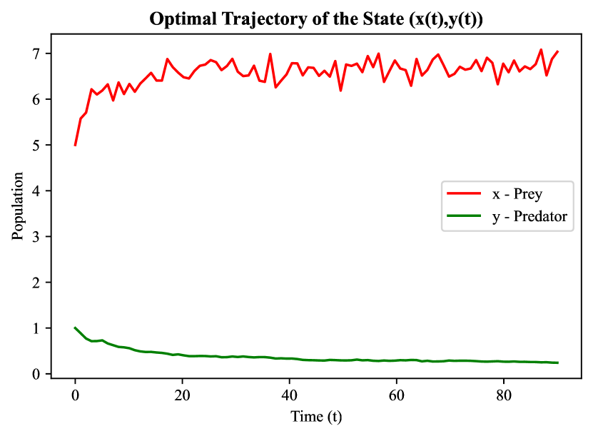
(a)

(b)

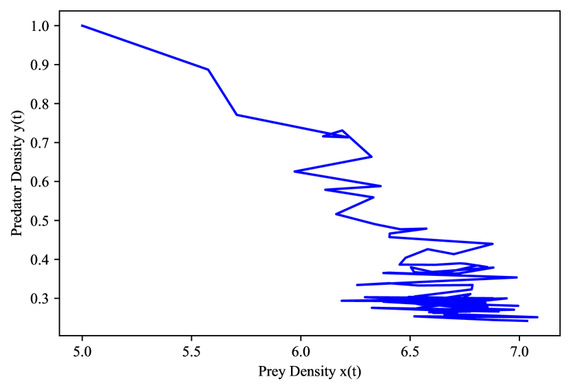
(c)

(d)

Figure 1: This figure depicts the optimal trajectory of the optimal control problem discussed in section 3.1 with the objective to drive the system from the initial state $(5,1)$ to the terminal state $(7,0.25)$. The parameter values for these plots are chosen to be $r=1,\gamma=7,g=0.4,m=0.37,\delta=0.1,\xi=0.1,A_{1}=A_{2}=A_{3}=1$. The terminal value of co-state variables is $(p_{1}(T),p_{2}(T))=(0,0)$. The intensities of noise are chosen as $\sigma_{1}=\sigma_{2}=0.02$. In order to account the randomness, the stochastic control problem is simulated for $5000$ times and the average is plotted in these figures. This example depicts the optimal quality of additional food required to achieve biological conservation, for a fixed quantity of food. The optimal control plot shows that the predators have to be given high quality of additional food initially and then the lower quality of food in order to conserve both the species from extinction. The desired terminal state is reached in $T=87$ units of time.

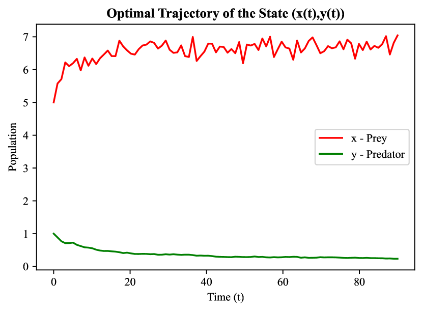
(a)

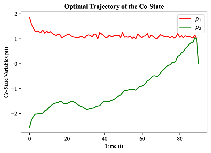
(b)

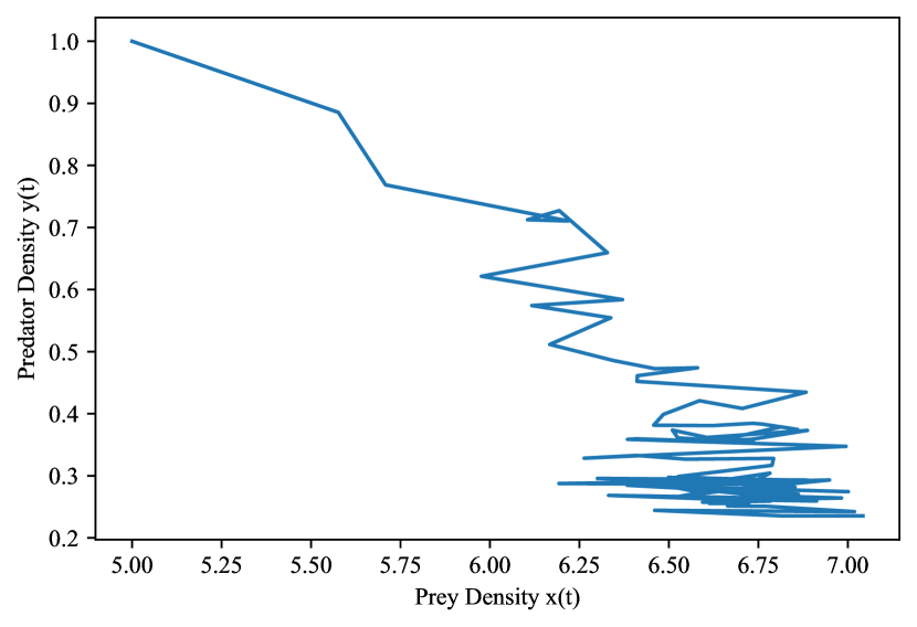
(c)

(d)

Figure 2: This figure depicts the optimal trajectory of the optimal control problem discussed in section 3.2 with the objective to drive the system from the initial state $(5,1)$ to the terminal state $(7,0.25)$. The parameter values for these plots are chosen to be $r=1,\gamma=7,g=0.4,m=0.37,\delta=0.1,\alpha=2,A_{1}=A_{2}=A_{3}=1$. The terminal value of co-state variables is $(p_{1}(T),p_{2}(T))=(0,0)$. The intensities of noise are chosen as $\sigma_{1}=\sigma_{2}=0.02$. In order to account the randomness, the stochastic control problem is simulated for $5000$ times and the average is plotted in these figures. This example depicts the optimal quantity of additional food required to achieve biological conservation, for a fixed quality of food. The optimal control plot shows that the predators have to be given high quantity of additional food initially and then the lower quantity of food in order to conserve both the species from extinction. The desired terminal state is reached in $T=84$ units of time.

4 Stochastic Time-Optimal Control Problem

In this section we wish to achieve pest eradication of nearly prey-elimination stage for the system (3) with quality and quantity of additional food as control variables in minimum time.

To attain this goal, we consider the following time optimal control probelem with the following objective functional along with the state equations (3)

$$J(u)=E\Bigg{[}\int_{0}^{T}1dt\Bigg{]}.$$ (17)

Here our goal is to find optimal controls $\alpha^{*}$ and $\xi^{*}$ such that $J(\alpha^{*},\xi^{*})\leq J(\alpha,\xi),\forall(\alpha(t),\xi(t))\in U$ where $U$ is an admissible control set defined by $U=\{(\alpha(t),\xi(t))|0\leq\alpha(t)\leq\alpha_{max},0\leq\xi(t)\leq\xi_{max}\forall t\in(0,t_{f}]\}$ where $(\alpha_{max},\xi_{max})\in(\mathcal{R}^{+})^{2}$

Now comparing the cost functional (17) with (5), we see that

$f(t,X(t),u(t))=1$ and $h(X(T))=0$.

Hence from the stochastic maximum principle, there exist stochastic processes

$(p(.),q(.))\in L_{F}^{2}(0,T;\mathcal{R}^{n})\times(L_{F}^{2}(0,T;\mathcal{R}^{n}))^{m},\ p(t)=\begin{pmatrix}p_{1}(t)\\ p_{2}(t)\end{pmatrix},\ q(t)=\begin{pmatrix}q_{1}(t)&q_{3}(t)\\ q_{2}(t)&q_{4}(t)\end{pmatrix}\ni$

$$\begin{split}\begin{pmatrix}dp_{1}(t)\\ dp_{2}(t)\end{pmatrix}&=-\Bigg{[}\begin{pmatrix}\frac{\partial b_{1}}{\partial x}&\frac{\partial b_{2}}{\partial x}\\ \frac{\partial b_{1}}{\partial y}&\frac{\partial b_{2}}{\partial y}\end{pmatrix}\begin{pmatrix}p_{1}(t)\\ p_{2}(t)\end{pmatrix}+\sigma_{X}^{1}(t,\bar{X}(t),\bar{u}(t))^{T}q_{1}(t)+\sigma_{X}^{2}(t,\bar{X}(t),\bar{u}(t))^{T}q_{2}(t)-\begin{pmatrix}\frac{\partial f}{\partial x}\\ \frac{\partial f}{\partial y}\end{pmatrix}\Bigg{]}dt\\ &+\begin{pmatrix}q_{1}(t)&q_{3}(t)\\ q_{2}(t)&q_{4}(t)\end{pmatrix}\begin{pmatrix}dW_{1}(t)\\ dW_{2}(t)\end{pmatrix}\\ p_{1}(T)&=0,\ p_{2}(T)=0\end{split}$$

Substituting $\frac{\partial f}{\partial x}=0,\frac{\partial f}{\partial y}=0$ and the values of $b_{X},\sigma_{X}^{1},\sigma_{X}^{2}$ from (10), (11), we see that the adjoint equations for the optimal controls $(\alpha^{*},\xi^{*})$ are given as:

$$\begin{split}dp_{1}(t)&=-\Bigg{[}\frac{\partial b_{1}}{\partial x}p_{1}(t)+\frac{\partial b_{2}}{\partial x}p_{2}(t)+\sigma_{1}q_{1}\Bigg{]}dt+q_{1}(t)dW_{1}(t)+q_{3}(t)dW_{2}(t)\\ dp_{2}(t)&=-\Bigg{[}\frac{\partial b_{1}}{\partial y}p_{1}(t)+\frac{\partial b_{2}}{\partial y}p_{2}(t)+\sigma_{2}q_{4}\Bigg{]}dt+q_{2}(t)dW_{1}(t)+q_{4}(t)dW_{2}(t)\\ p_{1}(T)&=0,\ p_{2}(T)=0\end{split}$$

On further simplification, we see that

$$\begin{split}dp_{1}(t)&=-\Bigg{[}\Big{(}r(1-\frac{2x}{\gamma})-\frac{2xy(1+\alpha\xi)}{(1+x^{2}+\alpha\xi)^{2}}\Big{)}p_{1}(t)+\frac{2gxy(1+(\alpha-1)\xi)}{(1+x^{2}+\alpha\xi)^{2}}p_{2}(t)+\sigma_{1}q_{1}\Bigg{]}dt\\ &+q_{1}(t)dW_{1}(t)+q_{3}(t)dW_{2}(t)\\ dp_{2}(t)&=-\Bigg{[}\frac{-x^{2}}{1+x^{2}+\alpha\xi}p_{1}(t)+\Big{(}g(\frac{x^{2}+\xi}{1+x^{2}+\alpha\xi})-m-2\delta y\Big{)}p_{2}(t)+\sigma_{2}q_{4}\Bigg{]}dt\\ &+q_{2}(t)dW_{1}(t)+q_{4}(t)dW_{2}(t)\\ p_{1}(T)&=0,\ p_{2}(T)=0\end{split}$$ (18)

The solutions of the above equations (12) gives $(p_{1}(t),p_{2}(t))$, which are the co-state vectors.

Now from (8), we see that the Hamiltonian for the system (3) is given by:

$$\begin{split}H(t,X,u,p,q)&=\left\langle p,b\right\rangle+tr[q^{T}\sigma]-1\\ &=\begin{pmatrix}p_{1}(t)&p_{2}(t)\end{pmatrix}\begin{pmatrix}b_{1}(t)\\ b_{2}(t)\end{pmatrix}+tr\Bigg{[}\begin{pmatrix}q_{1}(t)&q_{2}(t)\\ q_{3}(t)&q_{4}(t)\end{pmatrix}\begin{pmatrix}\sigma_{1}x&0\\ 0&\sigma_{2}y\end{pmatrix}\Bigg{]}-1\\ &=p_{1}(t)b_{1}+p_{2}(t)b_{2}+q_{1}\sigma_{1}x+q_{4}\sigma_{2}y-1\\ &=\Big{(}rx(t)(1-\frac{x(t)}{\gamma})-\frac{x^{2}(t)y(t)}{1+x^{2}(t)+\alpha\xi}\Big{)}p_{1}(t)+\Big{(}gy(t)(\frac{x^{2}(t)+\xi}{1+x^{2}(t)+\alpha\xi})-my(t)-\delta y^{2}(t)\Big{)}p_{2}(t)\\ &+q_{1}\sigma_{1}x+q_{4}\sigma_{2}y-1\\ \end{split}$$

Now from the Hamiltonian maximization condition (7), we have

$$\begin{split}\mathcal{H}(t,X^{*}(t),\alpha^{*}(t),\xi^{*}(t))&=\max_{(\alpha,\xi)\in U}H(t,X^{*}(t),\alpha(t),\xi(t))\\ \implies\frac{\partial H}{\partial\alpha}&=0,\ \frac{\partial H}{\partial\xi}=0\\ \end{split}$$

Considering

$$\begin{split}\frac{\partial H}{\partial\alpha}&=0\\ \implies&\frac{\partial}{\partial\alpha}\Big{(}rx(t)(1-\frac{x(t)}{\gamma})-\frac{x^{2}(t)y(t)}{1+x^{2}(t)+\alpha\xi}\Big{)}p_{1}+\frac{\partial}{\partial\alpha}\Big{(}gy(t)(\frac{x^{2}(t)+\xi}{1+x^{2}(t)+\alpha\xi})-my(t)-\delta y^{2}(t)\Big{)}p_{2}(t)\\ +&\frac{\partial}{\partial\alpha}(q_{1}\sigma_{1}x+q_{4}\sigma_{2}y-1)=0\\ \implies&\frac{\xi x^{2}yp_{1}}{(1+x^{2}+\alpha\xi)^{2}}-\frac{\xi gyp_{2}(x^{2}+\xi)}{(1+x^{2}+\alpha\xi)^{2}}=0\\ \implies&\xi gyp_{2}(x^{2}+\xi)-\xi x^{2}yp_{1}=0\\ \implies&\xi^{*}=\frac{p_{1}-gp_{2}}{gp_{2}}\end{split}$$

Similarly considering,

$$\begin{split}\frac{\partial H}{\partial\xi}&=0\\ \implies&\frac{\partial}{\partial\xi}\Big{(}rx(t)(1-\frac{x(t)}{\gamma})-\frac{x^{2}(t)y(t)}{1+x^{2}(t)+\alpha\xi}\Big{)}p_{1}+\frac{\partial}{\partial\xi}\Big{(}gy(t)(\frac{x^{2}(t)+\xi}{1+x^{2}(t)+\alpha\xi})-my(t)-\delta y^{2}(t)\Big{)}p_{2}(t)\\ +&\frac{\partial}{\partial\alpha}(q_{1}\sigma_{1}x+q_{4}\sigma_{2}y-1)=0\\ \implies&gyp_{2}(1+x^{2})+\alpha(x^{2}yp_{1}-gyp_{2}x^{2})=0\\ \implies&\alpha^{*}=\frac{gp_{2}(1+x^{2})}{x^{2}(gp_{2}-p_{1})}\end{split}$$

Hence the optimal quality and quantity variables for the stochastic time optimal control problem are given by

$(\alpha^{*},\xi^{*})=\{\frac{gp_{2}(1+x^{2})}{x^{2}(gp_{2}-p_{1})},\frac{p_{1}-gp_{2}}{gp_{2}}\}.$

4.1 Numerical Simulations

In this section, we numerically illustrate the theoretical findings of the above time optimal control problem with application to both biological conservation and pest management.

Using the Taylor series expansion, the time optimal control problem is simulated and plotted using the Stochastic Forward and Backward Sampling approach. The state equations (3) and the adjoint equations (12), (18) are solved using the forward and backward processes respectively. The forward process is simulated using the Euler-Maruyama scheme [26]. Among the various methods available to discretize the backward process, we chose an implicit scheme with a back propagation of the conditional expectations, which is of order $1/2$ [27]. These methods are implemented in Python using Sympy, Numpy and Matplotlib packages.

The sub plots present in the below figures 3 and 4 gives the optimal state trajectories, optimal co-state trajectories, phase diagram and optimal control trajectories respectively. These examples re-iterates the importance of additional food as control variables in the context of both ecological conservation and pest management.

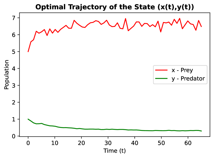
(a)

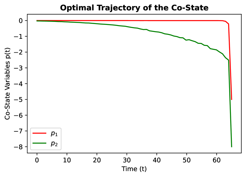
(b)

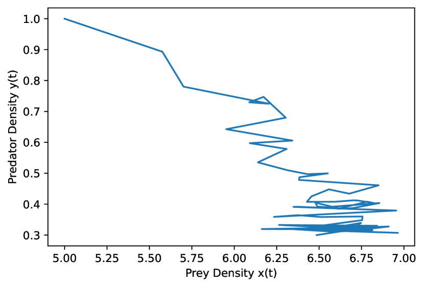
(c)

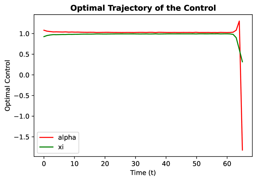
(d)

Figure 3: This figure depicts the optimal trajectory of the time-optimal control problem discussed in section 4 with the objective to drive the system from the initial state $(5,1)$ to the terminal state $(6.75,0.3)$ in minimum time. The parameter values for these plots are chosen to be $r=1,\gamma=7,g=0.4,m=0.37,\delta=0.1,\alpha=2,\xi=0.5$. The initial value of co-state variables is $(p_{1}(0),p_{2}(0))=(0,0)$. The intensities of noise are chosen as $\sigma_{1}=\sigma_{2}=0.02$. In order to account the randomness, the stochastic time-optimal control problem is simulated for $5000$ times and the average is plotted in these figures. This example depicts the optimal quality and quantity of additional food required to achieve biological conservation. The optimal control plot shows that the predators have to be given constant quantity of additional food ($1$ unit) and the constant quantity of additional food ($1$ unit) in order to conserve both the species from extinction. The desired terminal state is reached in $T=63$ units of time.

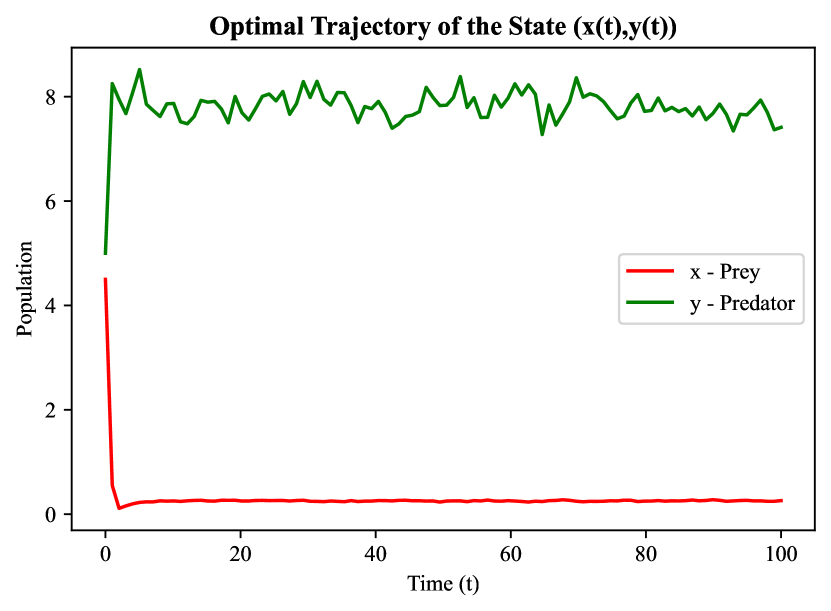
(a)

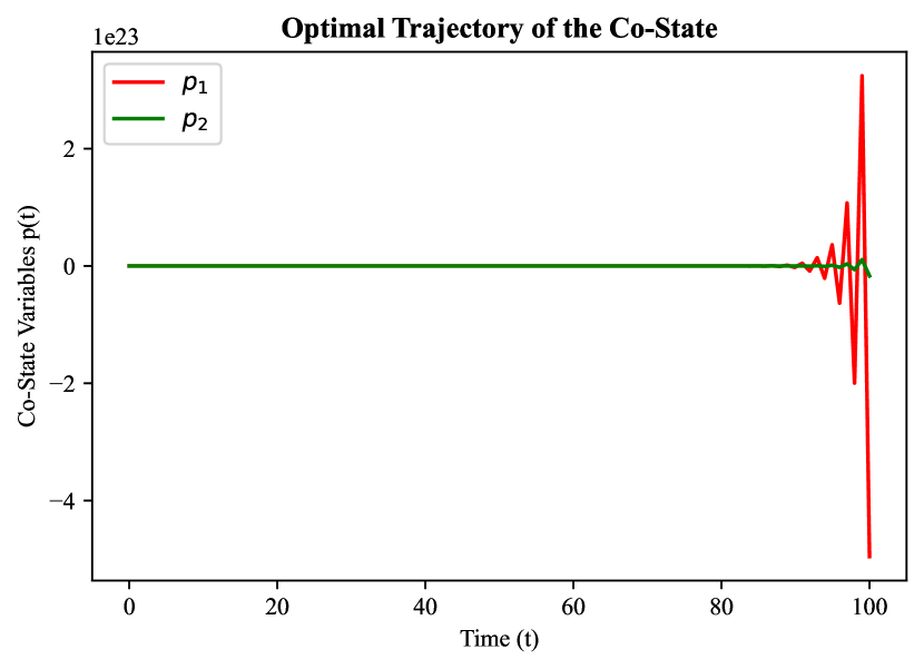
(b)

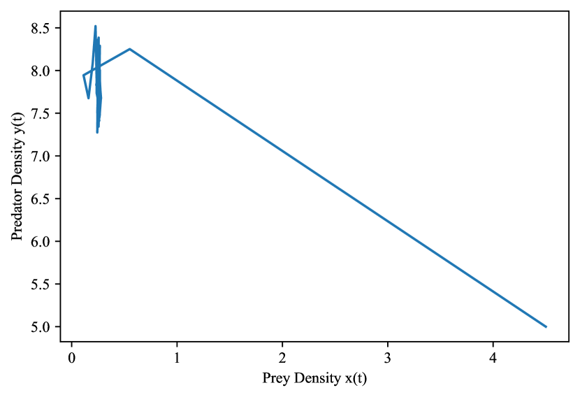
(c)

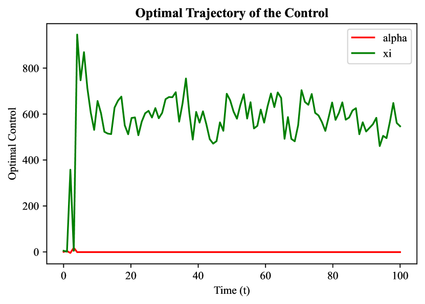
(d)

Figure 4: This figure depicts the optimal trajectory of the time-optimal control problem discussed in section 4 with the objective to drive the system from the initial state $(4.5,5)$ to the terminal state $(0.26,7.41)$ in minimum time. The parameter values for these plots are chosen to be $r=0.7,\gamma=5,g=1.2,m=0.19,\delta=0.05,\alpha=1.4,\xi=1.4$. The initial value of co-state variables is $(p_{1}(0),p_{2}(0))=(9,-6)$. The intensities of noise are chosen as $\sigma_{1}=\sigma_{2}=0.02$. In order to account the randomness, the stochastic time-optimal control problem is simulated for $5000$ times and the average is plotted in these figures. This example depicts the optimal quality and optimal quantity of additional food required to achieve pest management. The optimal control plot shows that the predators have to be given constant quality of additional food ($0.67$ units) and a high quantity of additional food throughout for reducing the pest population effectively. This example suggest that even with low quality of additional food and high quantity, the prey (pest) can be reduced to a threshold level at which they no longer cause significant damage to the ecosystem. The desired terminal state is reached in $T=100$ units of time.

5 Discussions and Conclusions

The provision of additional food has proven to be very effective in conserving endangered species [28, 29, 30] as well as controlling invasive or harmful species [31, 32, 33]. A significant amount of theoretical work was also done on the impact of additional food in various ecosystems [34, 23]. Both theoretically and experimentally, the technique of providing additional food for bio-control seemed to be very effective. Now a days researchers are also focusing on the the optimal additional food to be given to the predators. Some of the findings in this direction show that the quality and quantity of additional food provided play a crucial role in this optimal studies [24]. For instance, the authors in [11, 12] worked on the deterministic Holling type-III predator-prey systems and found the optimal quality and quantity of additional food required to drive the system to a desired terminal state.

It is a well known fact that the real-life systems behave more chaotic. Stochastic setting can be an ideal tool to capture such random system dynamics better than that of deterministic system dynamics. Motivated by the above discussions, in this work, we worked on a stochastic predator-prey system with additional food for predator and exhibiting Holling type-III functional response which in a way can be considered to be a generalization of the work [11, 12]. We have also incorporated the intra-specific competition among predators in the model to make the model more realistic.

In this work we initially considered a Lagrangian optimal control problem with a cost that is linear w.r.t. state and quadratic w.r.t. control with the end goal of biological conservation of both the species. We considered two cases with the quality of additional food and the quantity of additional food as control variables respectively. We calculated the optimal control values using stochastic maximum principle. We then numerically simulated using Forward-Backward Sampling method. These results showed that biological conservation of the system can be achieved by the optimal control strategy of providing the quality and the quantity of additional food high initially and further reducing them over the time.

Secondly, we studied a time-optimal control problem with the end goal of biological conservation of both the species and also to achieve the goal of pest management in minimum time. In this problem, we worked with a multi-dimensional control involving both the quality and quantity of additional food as control variables. The optimal control values are calculated using the stochastic maximum principle. We also plotted these solutions for two different set of parameters, one applied to biological conservation and the other to pest management. In case of biological conservation, both the controls did not exhibit any switch over the time. In case of pest management, optimal quality of the additional food remained low and constant throughout. The optimal quantity of additional food fluctuated initially and remained high throughout.

The present stochastic optimal control studies can further be improved by incorporating alley effect and even multiple prey and predator species to make the model more realistic. Also, the model presented here does not account for time delay. As diffusion term in this system is independent of control, the results obtained will be similar to that of deterministic case. It will be very interesting to take up problems with control in the diffusion. Since the current systems are of higher orders of non-linearity, it turns out that the numerical methods play a crucial role in understanding the chaotic behaviours. Hence, the study of higher-order numerical methods like Stochastic Runge-Kutta methods will enhance the output. Also not much work has been done where multiple noise are added simultaneously. We aim to take up these studies in the future.

Ethical Approval

This research did not require ethical approval.

Funding

This research was supported by National Board of Higher Mathematics(NBHM), Government of India(GoI) under project grant Time Optimal Control and Bifurcation Analysis of Coupled Nonlinear Dynamical Systems with Applications to Pest Management(02011/11/2021NBHM(R.P)/R$\&$D II/10074).

Conflicts of Interest

The authors have no conflicts of interest to disclose.

Acknowledgments

The authors dedicate this paper to the founder chancellor of SSSIHL, Bhagawan Sri Sathya Sai Baba. The corresponding author also dedicates this paper to his loving elder brother D. A. C. Prakash who still lives in his heart.

References

• [1] Alfred James Lotka “Elements of physical biology” Williams & Wilkins, 1925
• [2] Vito Volterra “Variazioni e fluttuazioni del numero d’individui in specie animali conviventi” C. Ferrari Venezia, 1927
• [3] Mark Kot “Elements of mathematical ecology” Cambridge University Press, 2001
• [4] Crawford Stanley Holling “The functional response of invertebrate predators to prey density” In The Memoirs of the Entomological Society of Canada 98.S48 Cambridge University Press, 1966, pp. 5–86
• [5] Joseph S Elkinton, Andrew M Liebhold and Rose-Marie Muzika “Effects of alternative prey on predation by small mammals on gypsy moth pupae” In Population Ecology 46.2 Springer, 2004, pp. 171–178
• [6] Valeria Fernández-Arhex and Juan C Corley “The functional response of Ibalia leucospoides (Hymenoptera: Ibaliidae), a parasitoid of Sirex noctilio (Hymenoptera: Siricidae)” In Biocontrol Science and Technology 15.2 Taylor & Francis, 2005, pp. 207–212
• [7] Andrew Yu Morozov “Emergence of Holling type III zooplankton functional response: bringing together field evidence and mathematical modelling” In Journal of theoretical biology 265.1 Elsevier, 2010, pp. 45–54
• [8] Stephen M Redpath and Simon J Thirgood “Numerical and functional responses in generalist predators: hen harriers and peregrines on Scottish grouse moors” In Journal of Animal Ecology 68.5 Wiley Online Library, 1999, pp. 879–892
• [9] P D N Srinivasu, D K K Vamsi and I Aditya “Biological conservation of living systems by providing additional food supplements in the presence of inhibitory effect: a theoretical study using predator–prey models” In Differential Equations and Dynamical Systems 26.1 Springer, 2018, pp. 213–246
• [10] P D N Srinivasu, D K K Vamsi and V S Ananth “Additional food supplements as a tool for biological conservation of predator-prey systems involving type III functional response: A qualitative and quantitative investigation” In Journal of theoretical biology 455 Elsevier, 2018, pp. 303–318
• [11] V S Ananth and D K K Vamsi “Influence of quantity of additional food in achieving biological conservation and pest management in minimum-time for prey-predator systems involving Holling type III response” In Heliyon 7.8 Elsevier, 2021, pp. e07699
• [12] V S Ananth and D K K Vamsi “Achieving Minimum-Time Biological Conservation and Pest Management for Additional Food provided Predator–Prey Systems involving Inhibitory Effect: A Qualitative Investigation” In Acta Biotheoretica 70.1 Springer, 2022, pp. 1–51
• [13] V S Ananth and D K K Vamsi “An Optimal Control Study with Quantity of Additional food as Control in Prey-Predator Systems involving Inhibitory Effect” In Computational and Mathematical Biophysics 9.1 De Gruyter Open Access, 2021, pp. 114–145
• [14] Mustapha Belabbas, Abdelghani Ouahab and Fethi Souna “Rich dynamics in a stochastic predator-prey model with protection zone for the prey and multiplicative noise applied on both species” In Nonlinear Dynamics 106.3 Springer, 2021, pp. 2761–2780
• [15] Sampurna Sengupta, Pritha Das and Debasis Mukherjee “Stochastic non-autonomous Holling type-III prey-predator model with predator’s intra-specific competition” In Discrete & Continuous Dynamical Systems-B 23.8 American Institute of Mathematical Sciences, 2018, pp. 3275
• [16] Xiaoxia Guo and Dehan Ruan “Extinction and ergodic stationary distribution of a Markovian-switching prey-predator model with additional food for predator” In Mathematical Modelling of Natural Phenomena 15 EDP Sciences, 2020, pp. 46
• [17] Lin Li and Wencai Zhao “Deterministic and stochastic dynamics of a modified Leslie-Gower prey-predator system with simplified Holling-type IV scheme” In Mathematical Biosciences and Engineering 18.3 AMER INST MATHEMATICAL SCIENCES-AIMS PO BOX 2604, SPRINGFIELD, MO 65801-2604 USA, 2021, pp. 2813–2831
• [18] Wen Qin, Hanjun Zhang and Qingsong He “Survival and ergodicity of a stochastic Holling-III predator–prey model with Markovian switching in an impulsive polluted environment” In Advances in Difference Equations 2021.1 Springer, 2021, pp. 1–19
• [19] XD Gu and WQ Zhu “Stochastic optimal control of predator–prey ecosystem by using stochastic maximum principle” In Nonlinear Dynamics 85.2 Springer, 2016, pp. 1177–1184
• [20] Awad El-Gohary and Fawzy A Bukhari “Optimal control of stochastic prey–predator models” In Applied mathematics and computation 146.2-3 Elsevier, 2003, pp. 403–415
• [21] Meng Liu “Optimal harvesting policy of a stochastic predator–prey model with time delay” In Applied Mathematics Letters 48 Elsevier, 2015, pp. 102–108
• [22] P D N Srinivasu and B S R V Prasad “Role of quantity of additional food to predators as a control in predator–prey systems with relevance to pest management and biological conservation” In Bulletin of mathematical biology 73.10 Springer, 2011, pp. 2249–2276
• [23] P D N Srinivasu and B S R V Prasad “Time optimal control of an additional food provided predator–prey system with applications to pest management and biological conservation” In Journal of mathematical biology 60.4 Springer, 2010, pp. 591–613
• [24] P D N Srinivasu, D K K Vamsi and V S Ananth “Additional food supplements as a tool for biological conservation of predator-prey systems involving type III functional response: A qualitative and quantitative investigation” In Journal of theoretical biology 455 Elsevier, 2018, pp. 303–318
• [25] Jiongmin Yong and Xun Yu Zhou “Stochastic controls: Hamiltonian systems and HJB equations” Springer Science & Business Media, 1999
• [26] Eckhard Platen and Nicola Bruti-Liberati “Numerical solution of stochastic differential equations with jumps in finance” Springer Science & Business Media, 2010
• [27] Jianfeng Zhang “A numerical scheme for BSDEs” In The annals of applied probability 14.1 Institute of Mathematical Statistics, 2004, pp. 459–488
• [28] James D Harwood, Keith D Sunderland and William OC Symondson “Prey selection by linyphiid spiders: molecular tracking of the effects of alternative prey on rates of aphid consumption in the field” In Molecular Ecology 13.11 Wiley Online Library, 2004, pp. 3549–3560
• [29] RJ Putman and Brian W Staines “Supplementary winter feeding of wild red deer Cervus elaphus in Europe and North America: justifications, feeding practice and effectiveness” In Mammal Review 34.4 Wiley Online Library, 2004, pp. 285–306
• [30] Stephen M Redpath, Simon J Thirgood and Fiona M Leckie “Does supplementary feeding reduce predation of red grouse by hen harriers?” In Journal of Applied Ecology 38.6 Wiley Online Library, 2001, pp. 1157–1168
• [31] Maurice W Sabelis and Paul CJ Van Rijn “When does alternative food promote biological pest control?” In IOBC WPRS BULLETIN 29.4 IOBC/WPRS; 1998, 2006, pp. 195
• [32] Mark R Wade, Myron P Zalucki, Steve D Wratten and Katherine A Robinson “Conservation biological control of arthropods using artificial food sprays: current status and future challenges” In Biological control 45.2 Elsevier, 2008, pp. 185–199
• [33] Karin Winkler, Felix L Wäckers, Attila Stingli and Joop C Van Lenteren “Plutella xylostella (diamondback moth) and its parasitoid Diadegma semiclausum show different gustatory and longevity responses to a range of nectar and honeydew sugars” In Entomologia Experimentalis et Applicata 115.1 Wiley Online Library, 2005, pp. 187–192
• [34] P D N Srinivasu, B S R V Prasad and M Venkatesulu “Biological control through provision of additional food to predators: a theoretical study” In Theoretical Population Biology 72.1 Elsevier, 2007, pp. 111–120