EGSDE: Unpaired Image-to-Image Translation via Energy-Guided Stochastic Differential Equations

Abstract

Score-based diffusion models (SBDMs) have achieved the SOTA FID results in unpaired image-to-image translation (I2I). However, we notice that existing methods totally ignore the training data in the source domain, leading to sub-optimal solutions for unpaired I2I. To this end, we propose energy-guided stochastic differential equations (EGSDE) that employs an energy function pretrained on both the source and target domains to guide the inference process of a pretrained SDE for realistic and faithful unpaired I2I. Building upon two feature extractors, we carefully design the energy function such that it encourages the transferred image to preserve the domain-independent features and discard domain-specific ones. Further, we provide an alternative explanation of the EGSDE as a product of experts, where each of the three experts (corresponding to the SDE and two feature extractors) solely contributes to faithfulness or realism. Empirically, we compare EGSDE to a large family of baselines on three widely-adopted unpaired I2I tasks under four metrics. EGSDE not only consistently outperforms existing SBDMs-based methods in almost all settings but also achieves the SOTA realism results without harming the faithful performance. Furthermore, EGSDE allows for flexible trade-offs between realism and faithfulness and we improve the realism results further (e.g., FID of 51.04 in Cat $\to$ Dog and FID of 50.43 in Wild $\to$ Dog on AFHQ) by tuning hyper-parameters. The code is available at https://github.com/ML-GSAI/EGSDE.

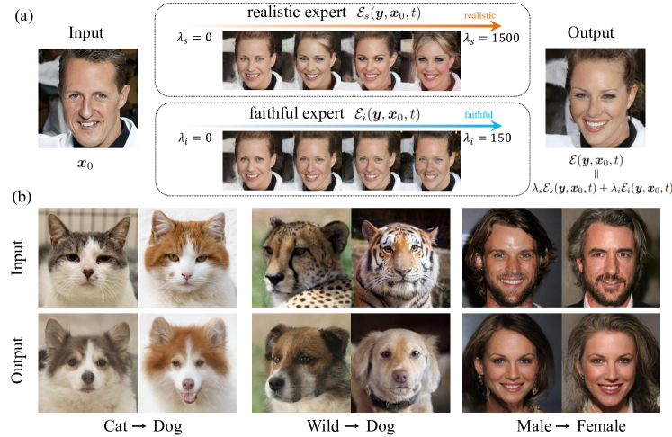
Figure 1: (a) Apart from the SDE, the EGSDE incorporates a realism expert and a faithful expert to preserve the domain-independent features and discard domain-specific ones. (b) Representative translation results on three unpaired I2I tasks.

1 Introduction

Unpaired image-to-image translation (I2I) aims to transfer an image from a source domain to a related target domain, which involves a wide range of computer vision tasks such as style transfer, super-resolution and pose estimation [35]. In I2I, the translated image should be realistic to fit the style of the target domain by changing the domain-specific features accordingly, and faithful to preserve the domain-independent features of the source image. Over the past few years, generative adversarial networks [12] (GANs)-based methods [10, 61, 55, 36, 3, 58, 44, 19, 17, 26, 10] dominated this field due to their ability to generate high-quality samples.

In contrast to GANs, score-based diffusion models (SBDMs) [49, 16, 34, 50, 2, 31] perturb data to a Gaussian noise by a diffusion process and learn the reverse process to transform the noise back to the data distribution. Recently, SBDMs achieved competitive or even superior image generation performance to GANs [9] and thus were naturally applied to unpaired I2I [7, 32], which have achieved the state-of-the-art FID [13] and KID [4] results empirically. However, we notice that these methods did not leverage the training data in the source domain at all. Indeed, they trained a diffusion model solely on the target domain and exploited the test source image during inference (see details in Sec. 2.2). Therefore, we argue that if the training data in the source domain can be exploited together with those in the target domain, one can learn domain-specific and domain-independent features to improve both the realism and faithfulness of the SBDMs in unpaired I2I.

To this end, we propose energy-guided stochastic differential equations (EGSDE) that employs an energy function pretrained across the two domains to guide the inference process of a pretrained SDE for realistic and faithful unpaired I2I. Formally, EGSDE defines a valid conditional distribution via a reverse time SDE that composites the energy function and the pretrained SDE. Ideally, the energy function should encourage the transferred image to preserve the domain-independent features and discard domain-specific ones. To achieve this, we introduce two feature extractors that learn domain-independent features and domain-specific ones respectively, and define the energy function upon the similarities between the features extracted from the transferred image and the test source image. Further, we provide an alternative explanation of the discretization of EGSDE in the formulation of product of experts [15]. In particular, the pretrained SDE and the two feature extractors in the energy function correspond to three experts and each solely contributes to faithfulness or realism.

Empirically, we validate our method on the widely-adopted AFHQ [8] and CelebA-HQ [20] datasets including Cat $\to$ Dog, Wild $\to$ Dog and Male $\to$ Female tasks. We compare to a large family of baselines, including the GANs-based ones [36, 61, 17, 26, 3, 10, 58, 59] and SBDMs-based ones [7, 32] under four metrics (e.g., FID). EGSDE not only consistently outperforms SBDMs-based methods in almost all settings but also achieves the SOTA realism results without harming the faithful performance. Furthermore, EGSDE allows for flexible trade-offs between realism and faithfulness and we improve the FID further (e.g., 51.04 in Cat $\to$ Dog and 50.43 in Wild $\to$ Dog ) by tuning hyper-parameters. EGSDE can also be extended to multi-domain translation easily.

2 Background

2.1 Score-based Diffusion Models

Score-based diffusion models (SBDMs) gradually perturb data by a forward diffusion process, and then reverse it to recover the data [50, 2, 48, 16, 9]. Let $q({\bm{y}}_{0})$ be the unknown data distribution on ${\mathbb{R}}^{D}$. The forward diffusion process $\{{\bm{y}}_{t}\}_{t\in[0,T]}$, indexed by time $t$, can be represented by the following forward SDE:

$$d{\bm{y}}={\bm{f}}({\bm{y}},t)dt+g(t)d{\bm{w}},$$ (1)

where ${\bm{w}}\in\mathbb{R}^{D}$ is a standard Wiener process, ${\bm{f}}(\cdot,t):\mathbb{R}^{D}\to\mathbb{R}^{D}$ is the drift coefficient and $g(t)\in\mathbb{R}$ is the diffusion coefficient. The $f({\bm{y}},t)$ and $g(t)$ is related into the noise size and determines the perturbation kernel $q_{t|0}({\bm{y}}_{t}|{\bm{y}}_{0})$ from time $0$ to $t$. In practice, the $f({\bm{y}},t)$ is usually affine so that the the perturbation kernel is a linear Gaussian distribution and can be sampled in one step.

Let $q_{t}({\bm{y}})$ be the marginal distribution of the SDE at time $t$ in Eq. (1). Its time reversal can be described by another SDE [50]:

$$\mathrm{d}{\bm{y}}=[{\bm{f}}({\bm{y}},t)-g(t)^{2}\nabla_{\bm{y}}\log q_{t}({\bm{y}})]\mathrm{d}t+g(t)\mathrm{d}\overline{{\bm{w}}},$$ (2)

where $\overline{{\bm{w}}}$ is a reverse-time standard Wiener process, and $\mathrm{d}t$ is an infinitesimal negative timestep. [50] adopts a score-based model ${\bm{s}}({\bm{y}},t)$ to approximate the unknown $\nabla_{\bm{y}}\log q_{t}({\bm{y}})$ by score matching, thus inducing a score-based diffusion model (SBDM), which is defined by a SDE:

$$\mathrm{d}{\bm{y}}=[{\bm{f}}({\bm{y}},t)-g(t)^{2}{\bm{s}}({\bm{y}},t)]\mathrm{d}t+g(t)\mathrm{d}\overline{{\bm{w}}}.$$ (3)

There are numerous SDE solver to solve the Eq. (3) to generate images. [50] discretizes it using the Euler-Maruyama solver. Formally, adopting a step size of $h$, the iteration rule from $s$ to $t=s-h$ is:

$${\bm{y}}_{t}={\bm{y}}_{s}-[{\bm{f}}({\bm{y}}_{s},s)-g(s)^{2}{\bm{s}}({\bm{y}}_{s},s)]h+g(s)\sqrt{h}{\bm{z}},\quad{\bm{z}}\sim{\mathcal{N}}({\bm{0}},{\bm{I}}).$$ (4)

2.2 SBDMs in Unpaired Image to Image Translation

Given unpaired images from the source domain ${\mathcal{X}}\subset\mathbb{R}^{D}$ and the target domain ${\mathcal{Y}}\subset\mathbb{R}^{D}$ as the training data, the goal of unpaired I2I is to transfer an image from the source domain to the target domain. Such a process can be formulated as designing a distribution $p({\bm{y}}_{0}|{\bm{x}}_{0})$ on the target domain ${\mathcal{Y}}$ conditioned on an image ${\bm{x}}_{0}\in{\mathcal{X}}$ to transfer. The translated image should be realistic for the target domain by changing the domain-specific features and faithful for the source image by preserving the domain-independent features.

ILVR [7] uses a diffusion model on the target domain for realism. Formally, ILVR starts from ${\bm{y}}_{T}\sim{\mathcal{N}}({\bm{0}},{\bm{I}})$ and samples from the diffusion model according to Eq. (4) to obtain ${\bm{y}}_{t}$. For faithfulness, it further refines ${\bm{y}}_{t}$ by adding the residual between the sample ${\bm{y}}_{t}$ and the perturbed source image ${\bm{x}}_{t}$ through a non-trainable low-pass filter

$${\bm{y}}_{t}\leftarrow{\bm{y}}_{t}+\Phi({\bm{x}}_{t})-\Phi({\bm{y}}_{t}),\quad{\bm{x}}_{t}\sim q_{t|0}({\bm{x}}_{t}|{\bm{x}}_{0}),$$ (5)

where $\Phi(\cdot)$ is a low-pass filter and $q_{t|0}(\cdot|\cdot)$ is the perturbation kernel determined by the forward SDE in Eq. (1).

Similarly, SDEdit [32] also adopts a SBDM on the target domain for realism, i.e., sampling from the SBDM according to Eq. (4). For faithfulness, SDEdit starts the generation process from the noisy source image ${\bm{y}}_{M}\sim q_{M|0}({\bm{y}}_{M}|{\bm{x}}_{0})$, where $M$ is a middle time between $0$ and $T$, and is chosen to preserve the original overall structure and discard local details. We use $p_{r1}({\bm{y}}_{0}|{\bm{x}}_{0})$ to denote the marginal distribution defined by such SDE conditioned on ${\bm{x}}_{0}$.

Notably, these methods did not leverage the training data in the source domain at all and thus can be sub-optimal in terms of both the realism and faithfulness in unpaired I2I.

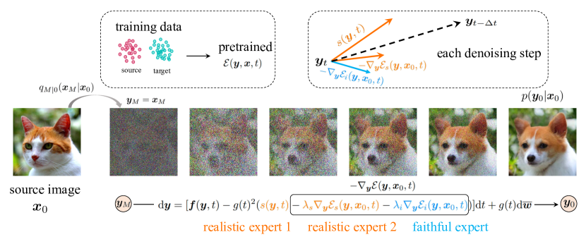
Figure 2: The overview of our EGSDE. Starting from the noisy source image, we can run the EGSDE for unpaired I2I, which employs an energy function ${\mathcal{E}}({\bm{y}},{\bm{x}},t)$ pretrained on both the source and target domains to guide the inference process of a pretrained SDE ($s({\bm{y}},t)$, realism expert 1). The energy function is decomposed into two terms further, where the realistic expert 2 ${\mathcal{E}}_{s}({\bm{y}},{\bm{x}},t)$ encourages the transferred image to discard domain-specific features and the faithful expert ${\mathcal{E}}_{i}({\bm{y}},{\bm{x}},t)$ aims to preserve the domain-independent ones.

3 Method

To overcome the limitations of existing methods [7, 32] as highlighted in Sec. 2.2, we propose energy-guided stochastic differential equations (EGSDE) that employs an energy function pre-trained across the two domains to guide the inference process of a pretrained SDE for realistic and faithful unpaired I2I (see Fig. 2). EGSDE defines a valid conditional distribution $p({\bm{y}}_{0}|{\bm{x}}_{0})$ by compositing a pretrained SDE and a pretrained energy function under mild regularity conditions as follows:

$$\mathrm{d}{\bm{y}}=[{\bm{f}}({\bm{y}},t)-g(t)^{2}({\bm{s}}({\bm{y}},t)-\nabla_{\bm{y}}{\mathcal{E}}({\bm{y}},{\bm{x}}_{0},t))]\mathrm{d}t+g(t)\mathrm{d}\overline{{\bm{w}}},$$ (6)

where $\overline{{\bm{w}}}$ is a reverse-time standard Wiener process, $\mathrm{d}t$ is an infinitesimal negative timestep, ${\bm{s}}(\cdot,\cdot):{\mathbb{R}}^{D}\times{\mathbb{R}}\rightarrow{\mathbb{R}}^{D}$ is the score-based model in the pretrained SDE and ${\mathcal{E}}(\cdot,\cdot,\cdot):{\mathbb{R}}^{D}\times{\mathbb{R}}^{D}\times{\mathbb{R}}\rightarrow{\mathbb{R}}$ is the energy function. The start point ${\bm{y}}_{M}$ is sampled from the perturbation distribution $q_{M|0}({\bm{y}}_{M}|{\bm{x}}_{0})$ [32], where $M=0.5T$ typically. We obtain the transferred images by taking the samples at endpoint $t=0$ following the SDE in Eq. (6).

Similar to the prior work [7, 32], EGSDE employs an SDE trained solely in the target domain as in Eq. (2), which defines a marginal distribution of the target images and mainly contributes to the realism of the transferred samples. In contrast, the energy function involves the training data across both the source and target domain, making EGSDE distinct from the prior work [7, 32]. Notably, although many other possibilities exist, we carefully design the energy function such that it (approximately) encourages the sample to retain the domain-independent features and discard the domain-specific ones to improve both the faithfulness and realism of the transferred sample. Below, we formally formulate the energy function.

3.1 Choice of Energy

In this section, we show how to design the energy function. Intuitively, during the translation, the domain-independent features (pose, color, etc. on Cat $\to$ Dog) should be preserved while the domain-specific features (beard, nose, etc. on Cat $\to$ Dog) should be changed accordingly. Motivated by this, we decompose the energy function ${\mathcal{E}}({\bm{y}},{\bm{x}},t)$ as the sum of two log potential functions [5]:

$${\mathcal{E}}({\bm{y}},{\bm{x}},t) =\lambda_{s}{\mathcal{E}}_{s}({\bm{y}},{\bm{x}},t)+\lambda_{i}{\mathcal{E}}_{i}({\bm{y}},{\bm{x}},t)$$ (7)

$$=\lambda_{s}\mathbb{E}_{q_{t|0}({\bm{x}}_{t}|{\bm{x}})}{\mathcal{S}}_{s}({\bm{y}},{\bm{x}}_{t},t)-\lambda_{i}\mathbb{E}_{q_{t|0}({\bm{x}}_{t}|{\bm{x}})}{\mathcal{S}}_{i}({\bm{y}},{\bm{x}}_{t},t),$$ (8)

where ${\mathcal{E}}_{i}(\cdot,\cdot,\cdot):\mathbb{R}^{D}\times\mathbb{R}^{D}\times\mathbb{R}\rightarrow\mathbb{R}$ and ${\mathcal{E}}_{s}(\cdot,\cdot,\cdot):\mathbb{R}^{D}\times\mathbb{R}^{D}\times\mathbb{R}\rightarrow\mathbb{R}$ are the log potential functions, ${\bm{x}}_{t}$ is the perturbed source image in the forward SDE, $q_{t|0}(\cdot|\cdot)$ is the perturbation kernel from time $0$ to time $t$ in the forward SDE, ${\mathcal{S}}_{s}(\cdot,\cdot,\cdot):\mathbb{R}^{D}\times\mathbb{R}^{D}\times\mathbb{R}\rightarrow\mathbb{R}$ and ${\mathcal{S}}_{i}(\cdot,\cdot,\cdot):\mathbb{R}^{D}\times\mathbb{R}^{D}\times\mathbb{R}\rightarrow\mathbb{R}$ are two functions measuring the similarity between the sample and perturbed source image, and $\lambda_{s}\in\mathbb{R}_{>0},\lambda_{i}\in\mathbb{R}_{>0}$ are two weighting hyper-parameters. Note that the expectation w.r.t. $q_{t|0}({\bm{x}}_{t}|{\bm{x}})$ in Eq. (7) guarantees that the energy function changes slowly over the trajectory to satisfy the regularity conditions in Appendix A.1.

To specify $\mathcal{S}_{s}(\cdot,\cdot,\cdot)$, we introduce a time-dependent domain-specific feature extractor $E_{s}(\cdot,\cdot):\mathbb{R}^{D}\times\mathbb{R}\rightarrow\mathbb{R}^{C\times H\times W}$, where $C$ is the channel-wise dimension, $H$ and $W$ are the dimension of height and width. In particular, $E_{s}(\cdot,\cdot)$ is the all but the last layer of a classifier that is trained on both domains to predict whether an image is from the source domain or the target domain. Intuitively, $E_{s}(\cdot,\cdot)$ will preserve the domain-specific features and discard the domain-independent features for accurate predictions. Building upon it, $\mathcal{S}_{s}(\cdot,\cdot,\cdot)$ is defined as the cosine similarity between the features extracted from the generated sample and the source image as follows:

$$\mathcal{S}_{s}({\bm{y}},{\bm{x}}_{t},t)=\frac{1}{HW}\sum_{h,w}\frac{E_{s}^{hw}({\bm{x}}_{t},t)^{\top}E_{s}^{hw}({\bm{y}},t)}{||E_{s}^{hw}({\bm{x}}_{t},t)||_{2}~{}||E_{s}^{hw}({\bm{y}},t)||_{2}},$$ (9)

where $E_{s}^{hw}(\cdot,\cdot)\in\mathbb{R}^{C}$ denote the channel-wise feature at spatial position $(h,w)$. Here we employ the cosine similarity since it preserves the spatial information and helps to improve the FID score empirically (see Appendix C.1 for the ablation study). Intuitively, reducing the energy value in Eq. (7) encourages the transferred sample to discard the domain-specific features to improve realism.

To specify $\mathcal{S}_{i}(\cdot,\cdot,\cdot)$, we introduce a domain-independent feature extractor $E_{i}(\cdot,\cdot):\mathbb{R}^{D}\times\mathbb{R}\rightarrow\mathbb{R}^{D}$, which is a low-pass filter. Intuitively, $E_{i}(\cdot,\cdot)$ will preserve the overall structures (i.e., domain-independent features) and discard local information like textures (i.e., domain-specific features). Building upon it, $\mathcal{S}_{i}(\cdot,\cdot,\cdot)$ is defined as the negative squared $L_{2}$ distance between the features extracted from the generated sample and source image as follows:

$$\mathcal{S}_{i}({\bm{y}},{\bm{x}}_{t},t)=-||E_{i}({\bm{y}},t)-E_{i}({\bm{x}}_{t},t)||_{2}^{2}.$$ (10)

Here, we choose negative squared $L_{2}$ distance as the similarity metric because it helps to preserve more domain-independent features empirically (see Appendix C.1 for the ablation study). Intuitively, reducing the energy value in Eq. (7) encourages the transferred sample to preserve the domain-independent features to improve faithfulness. In this paper we employ a low-pass filter for its simpleness and effectiveness while we can train more sophisticated $E_{i}$, e.g., based on disentangled representation learning methods [42, 6, 14, 23, 28], on the data in the two domains.

In our preliminary experiment, alternative to Eq. (7), we consider a simpler energy function that only involves the original source image ${\bm{x}}$ as follows:

$${\mathcal{E}}({\bm{y}},{\bm{x}},t) =\lambda_{s}\mathcal{S}_{s}({\bm{y}},{\bm{x}},t)-\lambda_{i}\mathcal{S}_{i}({\bm{y}},{\bm{x}},t),$$ (11)

which does not require to take the expectation w.r.t. ${\bm{x}}_{t}$. We found that it did not perform well because it is not reasonable to measure the similarity between the noise-free source image and the transferred sample in a gradual denoising process. See Appendix C.2 for empirical results.

3.2 Solving the Energy-guided Reverse-time SDE

Based on the pretrained score-based model ${\bm{s}}({\bm{y}},t)$ and energy function ${\mathcal{E}}({\bm{y}},{\bm{x}},t)$, we can solve the proposed energy-guided SDE to generate samples from conditional distribution $p({\bm{y}}_{0}|{\bm{x}}_{0})$. There are numerical solvers to approximate trajectories from SDEs. In this paper, we take the Euler-Maruyama solver following [32] for a fair comparison. Given the EGSDE as in Eq. (6) and adopting a step size $h$, the iteration rule from $s$ to $t=s-h$ is:

$${\bm{y}}_{t}={\bm{y}}_{s}-[{\bm{f}}({\bm{y}},s)-g(s)^{2}({\bm{s}}({\bm{y}}_{s},s)-\nabla_{\bm{y}}{\mathcal{E}}({\bm{y}}_{s},{\bm{x}}_{0},s))]h+g(s)\sqrt{h}{\bm{z}},\quad{\bm{z}}\sim{\mathcal{N}}({\bm{0}},{\bm{I}}).$$ (12)

The expectation in ${\mathcal{E}}({\bm{y}}_{s},{\bm{x}}_{0},s)$ is estimated by the Monte Carlo method of a single sample for efficiency. For brevity, we present the general sampling procedure of our method in Algorithm 1. In experiments, we use the variance preserve energy-guided SDE (VP-EGSDE) [50, 16] and the details are explained in Appendix A.3, where we can modify the noise prediction network to $\tilde{\epsilon}({\bm{y}},{\bm{x}}_{0},t)=\epsilon({\bm{y}},t)+\sqrt{\bar{\beta_{t}}}\nabla_{\bm{y}}{\mathcal{E}}({\bm{y}},{\bm{x}}_{0},t)$ and take it into the sampling procedure in DDPM [16]. Following SDEdit [32], we further extend this by repeating the Algorithm 1 $K$ times (see details in Appendix A.2). Further, we explain the connection with classifier guidance[9] in Appendix A.5.

Algorithm 1 EGSDE for unpaired image-to-image translation

0:  the source image ${\bm{x}}_{0}$, the initial time $M$, denoising steps $N$, weighting hyper-parameters $\lambda_{s},\lambda_{i}$, the similarity function ${\mathcal{S}}_{s}(\cdot,\cdot,\cdot),{\mathcal{S}}_{i}(\cdot,\cdot,\cdot)$, the score function ${\bm{s}}(\cdot,\cdot)$

  ${\bm{y}}\sim q_{M|0}({\bm{y}}|{\bm{x}}_{0})$ # the start point

  $h=\frac{M}{N}$

  for $i=N$ to $1$ do

     $s\leftarrow ih$

     ${\bm{x}}\sim q_{s|0}({\bm{x}}|{\bm{x}}_{0})$ # sample perturbed source image from the perturbation kernel

     ${\mathcal{E}}({\bm{y}},{\bm{x}},s)\leftarrow\lambda_{s}{\mathcal{S}}_{s}({\bm{y}},{\bm{x}},s)-\lambda_{i}{\mathcal{S}}_{i}({\bm{y}},{\bm{x}},s)$ # compute energy with one Monte Carlo

     ${\bm{y}}\leftarrow{\bm{y}}-[{\bm{f}}({\bm{y}},s)-g(s)^{2}({\bm{s}}({\bm{y}},s)-\nabla_{\bm{y}}{\mathcal{E}}({\bm{y}},{\bm{x}},s))]h$ # the update rule in Eq. (12)

     ${\bm{z}}\sim{\mathcal{N}}({\bm{0}},{\bm{I}})$ if $i>1$, else ${\bm{z}}={\bm{0}}$

     ${\bm{y}}\leftarrow{\bm{y}}+g(s)\sqrt{h}{\bm{z}}$

  end for

  ${\bm{y}}_{0}\leftarrow{\bm{y}}$

  return  ${\bm{y}}_{0}$

3.3 EGSDE as Product of Experts

Inspired by the posterior inference process in diffusion models [46], we present a product of experts [15] explanation for the discretized sampling process of EGSDE, which formalizes our motivation in an alternative perspective and provides insights on the role of each component in EGSDE.

We first define a conditional distribution $\tilde{p}({\bm{y}}_{t}|{\bm{x}}_{0})$ at time $t$ as a product of experts:

$$\tilde{p}({\bm{y}}_{t}|{\bm{x}}_{0})=\frac{p_{r1}({\bm{y}}_{t}|{\bm{x}}_{0})p_{e}({\bm{y}}_{t}|{\bm{x}}_{0})}{Z_{t}},$$ (13)

where $Z_{t}$ is the partition function, $p_{e}({\bm{y}}_{t}|{\bm{x}}_{0})\propto\exp(-{\mathcal{E}}({\bm{y}}_{t},{\bm{x}}_{0},t))$ and $p_{r1}({\bm{y}}_{t}|{\bm{x}}_{0})$ is the marginal distribution at time $t$ defined by SDEdit based on a pretrained SDE on the target domain.

To sample from $\tilde{p}({\bm{y}}_{t}|{\bm{x}}_{0})$, we need to construct a transition kernel $\tilde{p}({\bm{y}}_{t}|{\bm{y}}_{s})$, where $t=s-h$ and $h$ is small. Following [46], using the desirable equilibrium $\tilde{p}({\bm{y}}_{t}|{\bm{x}}_{0})=\int\tilde{p}({\bm{y}}_{t}|{\bm{y}}_{s})\tilde{p}({\bm{y}}_{s}|{\bm{x}}_{0})d{\bm{y}}_{s}$, we construct the $\tilde{p}({\bm{y}}_{t}|{\bm{y}}_{s})$ as follows:

$$\tilde{p}({\bm{y}}_{t}|{\bm{y}}_{s})=\frac{p({\bm{y}}_{t}|{\bm{y}}_{s})p_{e}({\bm{y}}_{t}|{\bm{x}}_{0})}{\tilde{Z}_{t}({\bm{y}}_{s})},$$ (14)

where $\tilde{Z}_{t}({\bm{y}}_{s})$ is the partition function and $p({\bm{y}}_{t}|{\bm{y}}_{s})={\mathcal{N}}({\bm{\mu}}({\bm{y}}_{s},h),\Sigma(s,h){\bm{I}})$ is the transition kernel of the pretrained SDE in Eq. (4), i.e., ${\bm{\mu}}({\bm{y}}_{s},h)={\bm{y}}_{s}-[{\bm{f}}({\bm{y}}_{s},s)-g(s)^{2}{\bm{s}}({\bm{y}}_{s},s)]h$ and $\Sigma(s,h)=g(s)^{2}h$. Assuming that ${\mathcal{E}}({\bm{y}}_{t},{\bm{x}}_{0},t)$ has low curvature relative to $\Sigma(s,h)^{-1}$, it can be approximated using Taylor expansion around ${\bm{\mu}}({\bm{y}}_{s},h)$ and further we can obtain

$$\tilde{p}({\bm{y}}_{t}|{\bm{y}}_{s})\approx{\mathcal{N}}({\bm{\mu}}({\bm{y}}_{s},h)-\Sigma(s,h)\nabla_{{\bm{y}}^{\prime}}{\mathcal{E}}({\bm{y}}^{\prime},{\bm{x}}_{0},t)|_{{\bm{y}}^{\prime}={\bm{\mu}}({\bm{y}}_{s},h)},\Sigma(s,h){\bm{I}}).$$ (15)

More details about derivation are available in Appendix A.4. We can observe the transition kernel $\tilde{p}({\bm{y}}_{t}|{\bm{y}}_{s})$ in (25) is equal to the discretization of our EGSDE in Eq. (12). Therefore, solving the energy-guided SDE in a discretization manner is approximately equivalent to drawing samples from a product of experts in Eq. (13). Note that ${\mathcal{E}}({\bm{y}}_{t},{\bm{x}}_{0},t)=\lambda_{s}{\mathcal{E}}_{s}({\bm{y}}_{t},{\bm{x}}_{0},t)+\lambda_{i}{\mathcal{E}}_{i}({\bm{y}}_{t},{\bm{x}}_{0},t)$, the $\tilde{p}({\bm{y}}_{t}|{\bm{x}}_{0})$ can be rewritten as:

$$\tilde{p}({\bm{y}}_{t}|{\bm{x}}_{0}) =\frac{p_{r1}({\bm{y}}_{t}|{\bm{x}}_{0})p_{r2}({\bm{y}}_{t}|{\bm{x}}_{0})p_{f}({\bm{y}}_{t}|{\bm{x}}_{0})}{Z_{t}},$$ (16)

where $p_{r2}({\bm{y}}_{t}|{\bm{x}}_{0})\propto\exp(-\lambda_{s}{\mathcal{E}}_{s}({\bm{y}}_{t},{\bm{x}}_{0},t))$, $p_{f}({\bm{y}}_{t}|{\bm{x}}_{0})\propto\exp(-\lambda_{i}{\mathcal{E}}_{i}({\bm{y}}_{t},{\bm{x}}_{0},t))$.

In Eq. (16), by setting $t=0$, we can explain that the transferred samples approximately follow the distribution defined by the product of three experts, where $p_{r1}({\bm{y}}_{t}|{\bm{x}}_{0})$ and $p_{r2}({\bm{y}}_{t}|{\bm{x}}_{0})$ are the realism experts and $p_{f}({\bm{y}}_{t}|{\bm{x}}_{0})$ is the faithful expert, corresponding to the score function $s({\bm{y}},t)$ and the log potential functions ${\mathcal{E}}_{s}({\bm{y}},{\bm{x}},t)$ and ${\mathcal{E}}_{i}({\bm{y}},{\bm{x}},t)$ respectively. Such a formulation clearly explains the role of each expert in EGSDE and supports our empirical results.

4 Related work

Apart from the prior work mentioned before, we discuss other related work including GANs-based methods for unpaired I2I and SBDMs-based methods for image translation.

GANs-based methods for Unpaired I2I. Although previous paired image translation methods have also achieved remarkable performances [18, 52, 51, 37, 56, 60], we mainly focus on unpaired image translation in this work. The methods for two-domain unpaired I2I are mainly divided into two classes: two-side and one-side mapping [35, 58]. In the two-side framework [61, 55, 25, 29, 27, 24, 11, 1, 54, 57, 21], the cycle-consistency constraint is the most widely-used strategy such as in CycleGAN [61], DualGAN [55] and DiscoGAN [25]. The key idea is that the translated image should be able to be reconstructed by an inverse mapping. More recently, there are numerical studies to improve this such as SCAN [27] and U-GAT-IT [24]. Specifically, U-GAT-IT [24] applies an attention module to let the generator and discriminator focus on more important regions instead of the whole regions through the auxiliary classifier. Since such bijective projection is too restrictive, several studies are devoted to one-side mapping [36, 3, 10, 61, 58, 38, 19]. One representative approach is to design some kind of geometry distance to preserve content [35]. For example, DistanceGAN [3] keeps the distances between images within domains. GCGAN [10] maintains geometry-consistency between input and output. CUT [36] maximizes the mutual information between the input and output using contrastive learning. LSeSim [58] learns spatially-correlative representation to preserve scene structure consistency via self-similarities.

SBDMs-based methods for Image Translation. Several studies leveraged SBDMs for image translation due to their powerful generative ability and achieved good results. For example, DiffusionCLIP [22] fine-tune the score network with CLIP [39] loss, which is applied on text-driven image manipulation, zero-shot image manipulation and multi-attribute transfer successfully. GLIDE [33] and SDG [30] has achieved great performance on text-to-image translation. As for I2I, SR3 [41] and Palette [40] learn a conditional SBDM and outperform state-of-art GANs-based methods on super-resolution, colorization and so on, which needs paired data. For unpaired I2I, UNIT-DDPM [43] learns two SBDMs and two domain translation models using cycle-consistency loss. Compared with it, our method only needs one SBDM on the target domain, which is a kind of one-side mapping. ILVR [7] and SDEdit [32] utilize a SBDM on the target domain and exploited the test source image to refine inference, which ignored the training data in the source domain. Compared with these methods, our method employs an energy function pretrained across both the source and target domains to improve the realism and faithfulness of translated images.

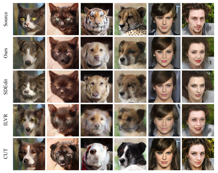
Figure 3: The qualitative comparison on Cat $\to$ Dog, Wild $\to$ Dog and Male $\to$ Female. Our method achieved better visual quality for both realism and faithfulness. For example, in the forth column, we successfully preserve the domain-independent features (i.e. green ground, pose and yellow color of body) and discard the domain-specific ones (i.e. leopard print).

5 Experiment

Datasets. We validated the EGSDE on following datasets, where all images are resized to $256\times 256$: (1) CelebA-HQ [20] contains high quality face images and is separated into two domains: male and female. Each category has 1000 testing images. We perform Male$\to$Female on this dataset.
(2) AFHQ [8] consists of high-resolution animal face images including three domains: cat, dog and wild, which has relatively large variations. Each domain has 500 testing images. We perform Cat$\to$Dog and Wild$\to$Dog on this dataset. We also perform multi-domain translation on AFHQ dataset and the experimental results are reported in Appendix D.

Implementation. The time-dependent domain-specific extractor $E_{s}({\bm{x}},t)$ is trained based on the backbone in [9]. The resize function including downsampling and upsampling operation is used as low-pass filter and is implemented by [45]. For generation process, by default, the weight parameter $\lambda_{s}$, $\lambda_{i}$ is set $500$ and $2$ respectively. The initial time $M$ and denoising steps $N$ is set $0.5T$ and $500$ by default. More details about implementation are available in Appendix B.

Evaluation Metrics. We evaluate translated images from two aspects: realism and faithfulness. For realism, we report the widely-used Frechet Inception Score (FID) [13] between translated images and the target dataset. To quantify faithfulness, we report the $L_{2}$ distance, PSNR and SSIM [53] between each input-output pair. To quantify both faithfulness and realism, we leverage Amazon Mechanical Turk(AMT) human evaluation to perform pairwise comparisons between the baselines and EGSDE. More details is available in Appendix B.6.

Table 1: Quantitative comparison. ILVR [7], SDEdit [32] and CUT [36] are reproduced using public code. StarGAN v2 [8] is evaluated by the provided public checkpoint and the other methods marked by * are public results from CUT[36] and ITTR [59]. All SBDMs-based methods and StarGAN v2 are repeated 5 times to eliminate randomness. CUT is conducted once since it learns a deterministic mapping. AMT show the preference rate of EGSDE against baselines via human evaluation. The EGSDE use the default-parameters ($\lambda_{s}=500,\lambda_{i}=2,M=0.5T$) and EGSDE^† use the parameters with $\lambda_{s}=700,\lambda_{i}=0.5,M=0.6T$.

Model	FID $\downarrow$	L2 $\downarrow$	PSNR $\uparrow$	SSIM $\uparrow$	AMT $\uparrow$
Cat $\to$ Dog
CycleGAN∗ [61]	85.9	-	-	-	-
MUNIT∗ [17]	104.4	-	-	-	-
DRIT∗ [26]	123.4	-	-	-	-
Distance∗ [3]	155.3	-	-	-	-
SelfDistance∗ [3]	144.4	-	-	-	-
GCGAN∗ [10]	96.6	-	-	-	-
LSeSim∗ [58]	72.8	-	-	-	-
ITTR (CUT)∗ [59]	68.6	-	-	-	-
StarGAN v2  [8]	54.88 ± 1.01	133.65 ± 1.54	10.63 ± 0.10	0.27 ± 0.003	-
CUT∗ [36]	76.21	59.78	17.48	0.601	79.6$\%$
ILVR [7]	74.37 ± 1.55	56.95 ± 0.14	17.77 ± 0.02	0.363 ± 0.001	75.4$\%$
SDEdit [32]	74.17 ± 1.01	47.88 ± 0.06	19.19 ± 0.01	0.423 ± 0.001	65.2$\%$
EGSDE	65.82 ± 0.77	47.22 ± 0.08	19.31 ± 0.02	0.415 ± 0.001	-
EGSDE†	51.04 ± 0.37	62.06 ± 0.10	17.17 ± 0.02	0.361 ± 0.001	-
Wild $\to$ Dog
CUT [36]	92.94	62.21	17.2	0.592	82.4$\%$
ILVR [7]	75.33 ± 1.22	63.40 ± 0.15	16.85 ± 0.02	0.287 ± 0.001	73.4$\%$
SDEdit [32]	68.51 ± 0.65	55.36 ± 0.05	17.98 ± 0.01	0.343 ± 0.001	57.2$\%$
EGSDE	59.75 ± 0.62	54.34 ± 0.08	18.14 ± 0.01	0.343 ± 0.001	-
EGSDE†	50.43± 0.52	66.52± 0.09	16.40± 0.01	0.300± 0.001	-
Male $\to$ Female
CUT [36]	31.94	46.61	19.87	0.74	58.6$\%$
ILVR [7]	46.12 ± 0.33	52.17 ± 0.10	18.59 ± 0.02	0.510 ± 0.001	88.2$\%$
SDEdit [32]	49.43 ± 0.47	43.70 ± 0.03	20.03 ± 0.01	0.572 ± 0.000	74.4$\%$
EGSDE	41.93 ± 0.11	42.04 ± 0.03	20.35 ± 0.01	0.574 ± 0.000	-
EGSDE†	30.61 ± 0.19	53.44 ± 0.09	18.32 ± 0.02	0.510 ± 0.001	-

5.1 Two-Domain Unpaired Image Translation

In this section, we compare EGSDE with the following state-of-the-art I2I methods in three tasks: SBDMs-based methods including ILVR [7] and SDEdit [32], and GANs-based methods including CUT [36], which are reproduced using public code. On the most popular benchmark Cat $\to$ Dog, we also report the performance of other state-of-the-art GANs-methods , where StarGAN v2 [8] is evaluated by the provided public checkpoint and the others are public results from CUT[36] and ITTR [59]. We provide more details about reproductions in Appendix B.7.

The quantitative comparisons and qualitative results are shown in Table 1 and Figure 3. We can derive several observations. First, our method outperforms the SBDMs-based methods significantly in almost all realism and faithfulness metrics, suggesting the effectiveness of employing energy function pretrained on both domains to guide the generation process. Especially, compared with the most direct competitor, i.e., SDEdit, with a lower $L_{2}$ distance at the same time, EGSDE improves the FID score by 8.35, 8.76 and 7.5 on Cat $\to$ Dog, Wild $\to$ Dog and Male $\to$ Female respectively. Second, EGSDE^† outperforms the current state-of-art GANs-based methods by a large margin on the challenging AFHQ dataset. For example, compared with CUT [36], we achieve an improvement of FID score with 25.17 and 42.51 on the Cat $\to$ Dog and Wild $\to$ Dog tasks respectively. In addition, the human evaluation shows that EGSDE are preferred compared to all baselines (> 50$\%$). The qualitative results in Figure 3 agree with quantitative comparisons in Table 1, where our method achieved the results with the best visual quality for both realism and faithfulness. We show more qualitative results and select some failure cases in Appendix C.6.

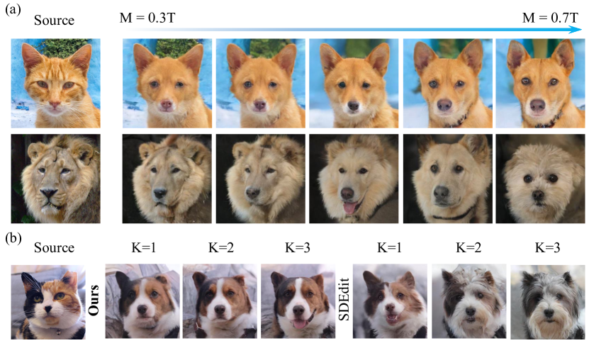
Figure 4: (a) The results of different initial time $M$. The larger $M$ results in more realistic and less faithful images. (b) The results of repeating the Algorithm 1 $K$ times. With the increase of K, SDEdit [32] tend to discard the domain-independent information of the source image (e.g., color and background) while our method still preserve them without harming realism.

5.2 Ablation Studies

The function of each expert. We validate the function of realistic expert ${\mathcal{E}}_{s}({\bm{y}},{\bm{x}},t)$ and faithful expert ${\mathcal{E}}_{i}({\bm{y}},{\bm{x}},t)$ by changing the weighting hyper-parameter $\lambda_{s}$ and $\lambda_{i}$. As shown in Table 5.2 and Figure  1, larger $\lambda_{s}$ results in more realistic images and larger $\lambda_{i}$ results in more faithful images. More results is available in Appendix C.5.

The choice of initial time $M$. We explore the effect of the initial time $M$ of EGSDE. As shown in Figure 4, the larger $M$ results in more realistic and less faithful image. More results is available in Appendix C.3.

Repeating $K$ Times. Following SDEdit [32], we show the results of repeating the Algorithm 1 $K$ times. The quantitative and qualitative results are depicted in Table 5.2 and Figure 4. The experimental results show the EGSDE outperforms SDEdit in each $K$ step in all metrics. With the increase of $K$, the SDEdit generates more realism images but the faithful metrics decrease sharply, because it only utilizes the source image at the initial time $M$. As shown in Figure 4, when $K$=3, SDEdit discard the domain-independent information of the source image (i.e., color and background) while our method still preserves them without harming realism.

tableComparison with SDEdit [32] under different $K$ times on Male $\to$ Female. The results on other tasks are reported in Appendix C.4. Methods K FID$\downarrow$ L2$\downarrow$ PSNR$\uparrow$ SSIM$\uparrow$ SDEdit [32] 1 49.95 43.71 20.03 0.572 EGSDE 42.17 42.07 20.35 0.573 SDEdit [32] 2 46.26 50.70 18.77 0.542 EGSDE 38.68 47.10 19.40 0.548 SDEdit [32] 3 45.19 55.03 18.08 0.527 EGSDE 37.55 49.63 18.96 0.536

tableThe results of different $\lambda_{s}$ and $\lambda_{i}$ on Wild $\to$ Dog. $\lambda_{s}=\lambda_{i}=0$ corresponds to SDEdit [32]. $\lambda_{s},\lambda_{i}$ FID$\downarrow$ L2$\downarrow$ PSNR $\uparrow$ SSIM$\uparrow$ $\lambda_{s}=0,\lambda_{i}=0$ 67.87 55.39 17.97 0.344 $\lambda_{s}=100,\lambda_{i}=0$ 60.80 56.19 17.85 0.341 $\lambda_{s}=500,\lambda_{i}=0$ 53.72 58.65 17.47 0.335 $\lambda_{s}=800,\lambda_{i}=0$ 53.01 60.02 17.27 0.331 $\lambda_{s}=0,\lambda_{i}=0.5$ 68.31 53.23 18.32 0.347 $\lambda_{s}=0,\lambda_{i}=2$ 71.10 51.99 18.52 0.349 $\lambda_{s}=0,\lambda_{i}=5$ 72.70 51.44 18.61 0.351

6 Conclusions and Discussions

In this paper, we propose energy-guided stochastic differential equations (EGSDE) for realistic and faithful unpaired I2I, which employs an energy function pretrained on both domains to guide the generation process of a pretrained SDE. Building upon two feature extractors, we carefully design the energy function to preserve the domain-independent features and discard domain-specific ones of the source image. We demonstrate the EGSDE by outperforming state-of-art I2I methods on three widely-adopted unpaired I2I tasks.

One limitation of this paper is we employ a low-pass filter as the domain-independent feature extractor for its simpleness and effectiveness while we can train more sophisticated extractor, e.g. based on disentangled representation learning methods [42, 6, 14, 23, 28], on the data in the two domains. We leave this issue in future work. In addition, we must take care to exploit the method to avoid the potential negative social impact (i.e., generating fake images to mislead people).

Appendix A Details about EGSDE

A.1 Assumptions about EGSDE

Notations. ${\bm{f}}(\cdot,\cdot):\mathbb{R}^{D}\times\mathbb{R}\to\mathbb{R}^{D}$ is the drift coefficient. $g(\cdot):\mathbb{R}\to\mathbb{R}$ is the diffusion coefficient. ${\bm{s}}(\cdot,\cdot):{\mathbb{R}}^{D}\times{\mathbb{R}}\rightarrow{\mathbb{R}}^{D}$ is the score-based model. ${\mathcal{E}}(\cdot,\cdot,\cdot):{\mathbb{R}}^{D}\times{\mathbb{R}}^{D}\times{\mathbb{R}}\rightarrow{\mathbb{R}}$ is the energy function. ${\bm{x}}_{0}$ is the given source image.

Assumptions. EGSDE defines a valid conditional distribution $p({\bm{y}}_{0}|{\bm{x}}_{0})$ under following assumptions:

• $\exists C>0,\forall t\in{\mathbb{R}},\forall{\bm{x}},{\bm{y}}\in\mathbb{R}^{D}:||f({\bm{x}},t)-f({\bm{y}},t)||_{2}\leq C||{\bm{x}}-{\bm{y}}||_{2}.$

• $\exists C>0,\forall t,s\in{\mathbb{R}},\forall{\bm{y}}\in\mathbb{R}^{D}:||f({\bm{y}},t)-f({\bm{y}},s)||_{2}\leq C|t-s|.$

• $\exists C>0,\forall t\in{\mathbb{R}},\forall{\bm{x}},{\bm{y}}\in\mathbb{R}^{D}:||{\bm{s}}({\bm{x}},t)-{\bm{s}}({\bm{y}},t)||_{2}\leq C||{\bm{x}}-{\bm{y}}||_{2}.$

• $\exists C>0,\forall t,s\in{\mathbb{R}},\forall{\bm{y}}\in\mathbb{R}^{D}:||{\bm{s}}({\bm{y}},t)-{\bm{s}}({\bm{y}},s)||_{2}\leq C|t-s|.$

• $\exists C>0,\forall t\in{\mathbb{R}},\forall{\bm{x}},{\bm{y}}\in\mathbb{R}^{D}:||\nabla_{\bm{x}}{\mathcal{E}}({\bm{x}},{\bm{x}}_{0},t)-\nabla_{\bm{y}}{\mathcal{E}}({\bm{y}},{\bm{x}}_{0},t)||_{2}\leq C||{\bm{x}}-{\bm{y}}||_{2}.$

• $\exists C>0,\forall t,s\in{\mathbb{R}},\forall{\bm{y}}\in\mathbb{R}^{D}:||\nabla_{\bm{y}}{\mathcal{E}}({\bm{y}},{\bm{x}}_{0},t)-\nabla_{\bm{y}}{\mathcal{E}}({\bm{y}},{\bm{x}}_{0},s)||_{2}\leq C|t-s|.$

• $\exists C>0,\forall t,s\in{\mathbb{R}}:|g(t)-g(s)|\leq C|t-s|.$

A.2 An Extention of EGSDE

Following SDEdit [32], we further extend the original EGSDE by repeating it $K$ times. The general sampling procedure is summarized in Algorithm 2.

Algorithm 2 An extention of EGSDE for unpaired image-to-image translation

0:  the source image ${\bm{x}}_{0}$, the initial time $M$, denoising steps $N$, weighting hyper-parameters $\lambda_{s},\lambda_{i}$, the similarity function ${\mathcal{S}}_{s}(\cdot,\cdot,\cdot),{\mathcal{S}}_{i}(\cdot,\cdot,\cdot)$, the score function ${\bm{s}}(\cdot,\cdot)$, repeating times $K$

  $h=\frac{M}{N}$

  ${\bm{y}}_{0}\leftarrow{\bm{x}}_{0}$

  for $k=1$ to $K$ do

     ${\bm{y}}\sim q_{M|0}({\bm{y}}|{\bm{y}}_{0})$ # the start point

     for $i=N$ to $1$ do

        $s\leftarrow ih$

        ${\bm{x}}\sim q_{s|0}({\bm{x}}|{\bm{x}}_{0})$ # sample perturbed source image from the perturbation kernel

        ${\mathcal{E}}({\bm{y}},{\bm{x}},s)\leftarrow\lambda_{s}{\mathcal{S}}_{s}({\bm{y}},{\bm{x}},s)-\lambda_{i}{\mathcal{S}}_{i}({\bm{y}},{\bm{x}},s)$ # compute energy with one Monte Carlo

        ${\bm{y}}\leftarrow{\bm{y}}-[{\bm{f}}({\bm{y}},s)-g(s)^{2}({\bm{s}}({\bm{y}},s)-\nabla_{\bm{y}}{\mathcal{E}}({\bm{y}},{\bm{x}},s))]h$

        ${\bm{z}}\sim{\mathcal{N}}({\bm{0}},{\bm{I}})$ if $i>1$, else ${\bm{z}}={\bm{0}}$

        ${\bm{y}}\leftarrow{\bm{y}}+g(s)\sqrt{h}{\bm{z}}$

     end for

     ${\bm{y}}_{0}\leftarrow{\bm{y}}$

  end for

  ${\bm{y}}_{0}\leftarrow{\bm{y}}$

  return  ${\bm{y}}_{0}$

A.3 Variance Preserve Energy-guided SDE (VP-EGSDE)

In this section, we show a specific EGSDE: variance preserve energy-guided SDE (VP-EGSDE) [50, 16], which is conducted in our experiments. The VP-EGSDE is defined as follows:

$$\mathrm{d}{\bm{y}}=[-\frac{1}{2}\beta(t){\bm{y}}-\beta(t)({\bm{s}}({\bm{y}},t)-\nabla_{\bm{y}}{\mathcal{E}}({\bm{y}},{\bm{x}}_{0},t))]\mathrm{d}t+\sqrt{\beta(t)}\mathrm{d}\overline{{\bm{w}}},$$ (17)

where ${\bm{x}}_{0}$ is the given source image, $\beta(\cdot):{\mathbb{R}}\rightarrow{\mathbb{R}}$ is a positive function, $\overline{{\bm{w}}}$ is a reverse-time standard Wiener process, $\mathrm{d}t$ is an infinitesimal negative timestep, ${\bm{s}}(\cdot,\cdot):{\mathbb{R}}^{D}\times{\mathbb{R}}\rightarrow{\mathbb{R}}^{D}$ is the score-based model in the pretrained SDE and ${\mathcal{E}}(\cdot,\cdot,\cdot):{\mathbb{R}}^{D}\times{\mathbb{R}}^{D}\times{\mathbb{R}}\rightarrow{\mathbb{R}}$ is the energy function. The perturbation kernel $q_{t|0}({\bm{y}}_{t}|{\bm{y}}_{0})$ is ${\mathcal{N}}({\bm{y}}_{0}e^{-\frac{1}{2}\int_{0}^{t}\beta(s)\mathrm{d}s},(1-e^{-\int_{0}^{t}\beta(s)\mathrm{d}s}){\bm{I}})$ and $\beta(t)=\beta_{min}+t(\beta_{max}-\beta_{min})$ in practice. Following [32, 16], we use $\beta_{min}=0.1,\beta_{max}=20$. The iteration rule from $s$ to $t=s-h$ of VP-EGSDE in Eq. (17) is:

$${\bm{y}}_{t}=\frac{1}{\sqrt{1-\beta(s)h}}({\bm{y}}_{s}+\beta(s)h({\bm{s}}({\bm{y}}_{s},s)-\nabla_{\bm{y}}{\mathcal{E}}({\bm{y}}_{s},{\bm{x}}_{0},s))+\sqrt{\beta(s)h}{\bm{z}},\quad{\bm{z}}\sim{\mathcal{N}}({\bm{0}},{\bm{I}}),$$ (18)

where $h$ is a small step size. [50] showed the iteration rule in Eq. (18) is equivalent to that using Euler-Maruyama solver when $h$ is small in Appendix E. In other words, the score network is modified to $\tilde{s}({\bm{y}},{\bm{x}}_{0},t)={\bm{s}}({\bm{y}},t)-\nabla_{\bm{y}}{\mathcal{E}}({\bm{y}},{\bm{x}}_{0},t)$ in EGSDE . Accordingly, we can modify the noise prediction network to $\tilde{\epsilon}({\bm{y}},{\bm{x}}_{0},t)=\epsilon({\bm{y}},t)+\sqrt{\bar{\beta_{t}}}\nabla_{\bm{y}}{\mathcal{E}}({\bm{y}},{\bm{x}}_{0},t)$ and take it into the sampling procedure in DDPM [16].

Algorithm 3 VP-EGSDE for unpaired image-to-image translation

0:  the source image ${\bm{x}}_{0}$, the initial time $M$, denoising steps $N$, weighting hyper-parameters $\lambda_{s},\lambda_{i}$, the similarity function ${\mathcal{S}}_{s}(\cdot,\cdot,\cdot),{\mathcal{S}}_{i}(\cdot,\cdot,\cdot)$, the score function ${\bm{s}}(\cdot,\cdot)$

  ${\bm{y}}\sim q_{M|0}({\bm{y}}|{\bm{x}}_{0})$ # the start point

  $h=\frac{M}{N}$

  for $i=N$ to $1$ do

     $s\leftarrow ih$

     ${\bm{x}}\sim q_{s|0}({\bm{x}}|{\bm{x}}_{0})$ # sample perturbed source image from the perturbation kernel

     ${\mathcal{E}}({\bm{y}},{\bm{x}},s)\leftarrow\lambda_{s}{\mathcal{S}}_{s}({\bm{y}},{\bm{x}},s)-\lambda_{i}{\mathcal{S}}_{i}({\bm{y}},{\bm{x}},s)$ # compute energy with one Monte Carlo

     ${\bm{y}}\leftarrow\frac{1}{\sqrt{1-\beta(s)h}}({\bm{y}}+\beta(s)h({\bm{s}}({\bm{y}}_{s},s)-\nabla_{\bm{y}}{\mathcal{E}}({\bm{y}}_{s},{\bm{x}},s))$ # the update rule in Eq. (18)

     ${\bm{z}}\sim{\mathcal{N}}({\bm{0}},{\bm{I}})$ if $i>1$, else ${\bm{z}}={\bm{0}}$

     ${\bm{y}}\leftarrow{\bm{y}}+\sqrt{\beta(s)h}{\bm{z}}$

  end for

  ${\bm{y}}_{0}\leftarrow{\bm{y}}$

  return  ${\bm{y}}_{0}$

A.4 EGSDE as Product of Experts

In this section, we provide more details about the product of experts [15] explanation for the discretized sampling process of EGSDE. Recall that we construct the $\tilde{p}({\bm{y}}_{t}|{\bm{y}}_{s})$ as follows:

$$\tilde{p}({\bm{y}}_{t}|{\bm{y}}_{s})=\frac{p({\bm{y}}_{t}|{\bm{y}}_{s})p_{e}({\bm{y}}_{t}|{\bm{x}}_{0})}{\tilde{Z}_{t}({\bm{y}}_{s})},$$ (19)

where $\tilde{Z}_{t}({\bm{y}}_{s})$ is the partition function, $p({\bm{y}}_{t}|{\bm{y}}_{s})={\mathcal{N}}({\bm{\mu}}({\bm{y}}_{s},h),\Sigma(s,h){\bm{I}})$ is the transition kernel of the pretrained SDE, i.e., ${\bm{\mu}}({\bm{y}}_{s},h)={\bm{y}}_{s}-[{\bm{f}}({\bm{y}}_{s},s)-g(s)^{2}{\bm{s}}({\bm{y}}_{s},s)]h$ and $\Sigma(s,h)=g(s)^{2}h$. For brevity, we denote ${\bm{\mu}}={\bm{\mu}}({\bm{y}}_{s},h),\Sigma=\Sigma(s,h)$. Assuming that ${\mathcal{E}}({\bm{y}}_{t},{\bm{x}}_{0},t)$ has low curvature relative to $\Sigma^{-1}$, then we can use Taylor expansion around ${\bm{\mu}}$ to approximate it:

$${\mathcal{E}}({\bm{y}}_{t},{\bm{x}}_{0},t)\approx{\mathcal{E}}({\bm{\mu}},{\bm{x}}_{0},t)+({\bm{y}}_{t}-{\bm{\mu}})^{\top}{\bm{g}},$$ (20)

where ${\bm{g}}=\nabla{\bm{y}}^{\prime}{\mathcal{E}}({\bm{y}}^{\prime},{\bm{x}}_{0},t)|_{{\bm{y}}^{\prime}={\bm{\mu}}}$. Taking it into Eq. (19), we can get:

$$\log\tilde{p}({\bm{y}}_{t}|{\bm{y}}_{s}) \approx-\frac{1}{2}({\bm{y}}_{t}-{\bm{\mu}})^{\top}\Sigma^{-1}({\bm{y}}_{t}-{\bm{\mu}})-({\bm{y}}_{t}-{\bm{\mu}})^{\top}{\bm{g}}+constant$$ (21)

$$=-\frac{1}{2}{\bm{y}}_{t}^{\top}\Sigma^{-1}{\bm{y}}_{t}+\frac{1}{2}{\bm{y}}_{t}^{\top}\Sigma^{-1}{\bm{\mu}}+\frac{1}{2}{\bm{\mu}}^{\top}\Sigma^{-1}{\bm{y}}_{t}$$ (22)

$$-\frac{1}{2}{\bm{y}}^{\top}\Sigma^{-1}\Sigma{\bm{g}}-\frac{1}{2}{\bm{g}}^{\top}\Sigma\Sigma^{-1}{\bm{y}}+constant$$ (23)

$$=-\frac{1}{2}({\bm{y}}_{t}-{\bm{\mu}}+\Sigma{\bm{g}})^{\top}\Sigma^{-1}({\bm{y}}_{t}-{\bm{\mu}}+\Sigma{\bm{g}})+constant.$$ (24)

Therefore,

$$\tilde{p}({\bm{y}}_{t}|{\bm{y}}_{s}) \approx{\mathcal{N}}({\bm{\mu}}-\Sigma{\bm{g}},\Sigma{\bm{I}})$$ (25)

$$={\mathcal{N}}({\bm{\mu}}-\Sigma\nabla_{{\bm{y}}^{\prime}}{\mathcal{E}}({\bm{y}}^{\prime},{\bm{x}}_{0},t)|_{{\bm{y}}^{\prime}={\bm{\mu}}},\Sigma{\bm{I}}).$$ (26)

Therefore, solving the EGSDE in a discretization manner is approximately equivalent to drawing samples from a product of experts.

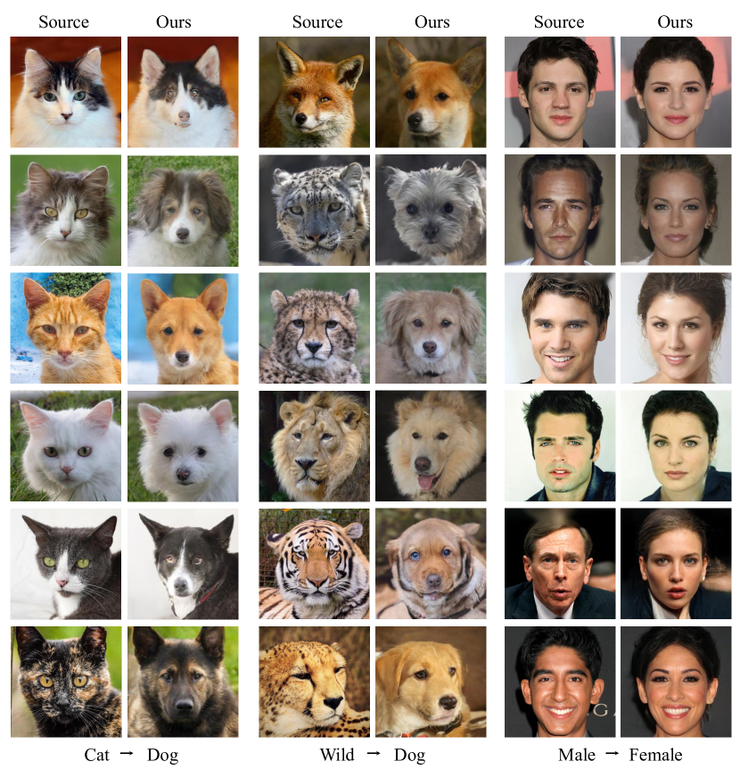
Figure 5: More qualitative results on three unpaired I2I tasks.

A.5 The Connection with Classifier Guidance

In this section, we show the classifier guidance[9] can be regarded as a special design of energy function and provide an alternative explanation of the classifier guidance as a product of experts.

Recall that the EGSDE, which leverages an energy function to guide the inference process of a pretrained SDE, is defined as follows:

$$\mathrm{d}{\bm{x}}=[{\bm{f}}({\bm{x}},t)-g(t)^{2}({\bm{s}}({\bm{x}},t)-\nabla_{\bm{x}}{\mathcal{E}}({\bm{x}},c,t))]\mathrm{d}t+g(t)\mathrm{d}\overline{{\bm{w}}},$$ (27)

which defines a distribution $p({\bm{x}}_{0}|c)$ conditioned on c. Let ${\mathcal{E}}({\bm{x}},c,t)\varpropto-\log p_{t}(c|{\bm{x}})^{\lambda}$, where $p_{t}(c|{\bm{x}})$ is a time-dependent classifier and $c$ is the class label, the EGSDE can be rewritten as:

$$\mathrm{d}{\bm{x}}=[{\bm{f}}({\bm{x}},t)-g(t)^{2}({\bm{s}}({\bm{x}},t)+\lambda\nabla_{\bm{x}}\log p_{t}(c|{\bm{x}}))]\mathrm{d}t+g(t)\mathrm{d}\overline{{\bm{w}}}.$$ (28)

Sovling variance preserve energy-guided SDE (VP-EGSDE) in Eq. 28 with Euler-Maruyama solver is equal to the classifier guidance in [9, 50].

Assuming $\int e^{-{\mathcal{E}}({\bm{x}},c,t)}d{\bm{x}}<\infty$, we can define a conditional distribution $q_{t}({\bm{x}}|c)$ at time $t$ as follows:

$$q_{t}({\bm{x}}|c)=\frac{e^{-{\mathcal{E}}({\bm{x}},c,t)}}{\int e^{-{\mathcal{E}}({\bm{x}},c,t)}d{\bm{x}}}$$ (29)

According to the analysis in section 3.3, solving the EGSDE in Eq. 28 is approximately equivalent to drawing samples from a product of experts as follows:

$$\tilde{p}_{t}({\bm{x}}|c)=\frac{p_{t}({\bm{x}})q_{t}({\bm{x}}|c)}{Z_{t}},$$ (30)

where $p_{t}({\bm{x}})$ is the marginal distribution at time $t$ defined by a pretrained SDE. Therefore, the generated samples in classifier guidance approximately follow the distribution:

$$\tilde{p}_{0}({\bm{x}}|c)=\frac{p_{0}({\bm{x}})q_{0}({\bm{x}}|c)}{Z_{0}}.$$ (31)

Similarly, combining a conditional socre-based model and a classifier in [9] is approximately equivalent to drawing samples from a product of experts as follows:

$$\tilde{p}_{0}({\bm{x}}|c)=\frac{p_{0}({\bm{x}}|c)q_{0}({\bm{x}}|c)}{Z_{0}},$$ (32)

where $p_{0}({\bm{x}}|c)$ is the marginal distribution at time $t$ defined by a pretrained SDE.

Appendix B Implementation Details

B.1 Datasets

To validate our method, we conduct experiments on the following datasets:

(1) CelebA-HQ [20] contains high quality face images and is separated into two domains: male and female. For training data, it contains 10057 male images and 17943 female images. Each category has 1000 testing images. Male$\to$Female task was conducted on this dataset.

(2) AFHQ [8] consists of high-resolution animal face images including three domains: cat, dog and wild, which has relatively large variations. For training data, it contains 5153, 4739 and 4738 images for cat, dog and wild respectively. Each domain has 500 testing images. We performed Cat$\to$Dog, Wild$\to$Dog and multi-domain translation on this dataset.

During training, all images are resized 256$\times$256, randomHorizontalFliped with p = 0.5, and scaled to $[-1,1]$. During sampling, all images are resized 256$\times$256 and scaled to $[-1,1]$.

Table 2: The used codes and license.

URL	citations	License
https://github.com/openai/guided-diffusion	[9]	MIT License
https://github.com/taesungp/contrastive-unpaired-translation	[36]	BSD License
https://github.com/jychoi118/ilvr$\_$adm	[7]	MIT License
https://github.com/ermongroup/SDEdit	[32]	MIT License
https://github.com/mseitzer/pytorch-fid	[13]	Apache V2.0 License

B.2 Code Used and License

All used codes in this paper and its license are listed in Table 2.

B.3 Details of the Score-based Diffusion Model

On Cat$\to$Dog and Wild$\to$Dog, we use the public pre-trained score-based diffusion model (SBDM) provided in the official code https://github.com/jychoi118/ilvr$\_$adm of ILVR [7]. The pretrained model includes the variance and mean networks and we only use the mean network.

On Male $\to$ Female, we trained a SBDM for $1M$ iterations on the training set of female category using the recommended training code by SDEdit https://github.com/ermongroup/ddim. We use the same setting as SDEdit [32] and DDIM [47] for a fair comparison, where the models is trained with a batch size of $64$, a learning rate of $0.00002$, the Adam optimizer with $\beta_{1}=0.9$, $\beta_{2}=0.999$ and grad clip = 1.0, an exponential moving average (EMA) with a rate of 0.9999. The U-Net architecture is the same as [16]. The timesteps $N$ is 1000 and the noise schedule is linear as described in A.3.

B.4 Details of the Domain-specific Feature Extractor

The domain-specific feature extractor $E_{s}(\cdot,\cdot)$ is the all but the last layer of a classifier that is trained on both the source and target domains. The time-dependent classifier is trained using the official code https://github.com/openai/guided-diffusion of [9]. We use the ImageNet (256$\times$256) pretrained classifier provided in https://github.com/openai/guided-diffusion as the initial weight and train $5K$ iterations for two-domain I2I and $10K$ iterations for multi-domain I2I. We train the classifier with a batch size of $32$, a learning rate of $3e-4$ with the AdamW optimizer (weight decay = 0.05). For the architecture, the depth is set to 2, the channels is set to 128, the attention resolutions is set to 32,16,8 and the other hyperparameters are the default setting. The timesteps $N$ is 1000 and the noise schedule is linear.

Table 3: Computation cost comparison.

Methods	sec/iter$\downarrow$	Mem(GB)$\downarrow$
CUT	0.24	2.91
ILVR	60	1.84
SDEdit	33	2.20
EGSDE	85	3.64

B.5 Training and Inference Time

On Cat $\to$ Dog, training the domain-specific feature extractor for $5K$ iterations takes 7 hours based on 5 2080Ti GPUs. The computation cost comparison for sampling is shown in Table 3, where the batch size is set 1. Compared with the ILVR, ours takes 1.42 times as long as ILVR. The speed of inference can be improved further by the latest progress on faster sampling [47, 2].

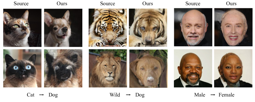
Figure 6: Selected failure cases. On Cat $\to$ Dog, the EGSDE sometimes fails to generate eyes and noses. On Wild $\to$ Dog, the EGSDE sometimes preserves some undesired features of the source image like tiger stripes. On Male $\to$ Female, the EGSDE fails to change the hairstyle.

B.6 Evaluation

FID. We evaluate the FID metric using the code https://github.com/mseitzer/pytorch-fid. On AFHQ dataset, following CUT [36], we use the test data as reference without any data preprocessing. On CelebA-HQ dataset, following StarGANv2 [36], we use the training data as reference and conduct the following data preprocessing: resize images to 256, 299 and then normalize data with $mean=0.485,0.456,0.406,std=0.229,0.224,0.225$. Note that the FID evaluation in StarGANv2 is still different with ours because it generates 10 images for each source image.

Human evaluation. We evaluate the human preference from both faithfulness and realism aspects via the Amazon Mechanical Turk (AMT). Given a source image, the AMT workers are instructed to select which translated image is more satisfactory in the pairwise comparisons between the baselines and EGSDE. The reward for each pair of picture comparison is kept as 0.02$\$$. Since each task takes around 4 s, the wage is around 18$\$$ per hour.

B.7 Reproductions

All baselines are reproduced based on the public code. Specifically, CUT [36] is reproduced based on the official code https://github.com/taesungp/contrastive-unpaired-translation. On Cat$\to$Dog, we use the public pretrained model directly without training. Following the setting on Cat$\to$Dog, we train the CUT $~{}2M$ iterations for other tasks. ILVR [7] is reproduced using the official code https://github.com/jychoi118/ilvr$\_$adm. The diffusion steps is set to 1000. The $down\_N$ of low-pass filter is set to 32. The $range\_t$ is set to 20. SDEdit [32] is reproduced using the official code https://github.com/ermongroup/SDEdit, where we use the default setting. For StarGANv2, we use the public checkpoint in https://github.com/clovaai/stargan-v2 for evaluation.

Appendix C Ablation Studies

C.1 Choice of the Similarity Metrics

Table 4: The results of different similarity metrics. NS $L_{2}$ denote negative square $L_{2}$ distance. Cosine similarity for ${\mathcal{S}}_{s}$ and NS $L_{2}$ for ${\mathcal{S}}_{i}$ is the default setting.

${\mathcal{S}}_{s}$	${\mathcal{S}}_{i}$	$\lambda_{s}$	$\lambda_{i}$	FID $\downarrow$	L2 $\downarrow$	PSNR $\uparrow$	SSIM $\uparrow$
Cosine	Cosine	500	500	61.47	52.16	18.69	0.407
Cosine	Cosine	500	10000	64.23	50.97	18.89	0.408
NS $L_{2}$	NS $L_{2}$	5e-07	2	77.01	45.91	19.84	0.431
NS $L_{2}$	NS $L_{2}$	5e-05	2	65.90	51.05	18.89	0.403
Cosine	NS $L_{2}$	500	2	65.23	47.15	19.32	0.415
Cosine	NS $L_{2}$	500	1	63.78	47.88	19.19	0.413

In this section, we perform two popular similarity metrics: cosine similarity and negative squared $L_{2}$ distance, for the similarity function ${\mathcal{S}}_{s}(\cdot,\cdot,\cdot)$ and ${\mathcal{S}}_{i}(\cdot,\cdot,\cdot)$. As shown in Table 4, the cosine similarity for ${\mathcal{S}}_{s}(\cdot,\cdot,\cdot)$ helps to improve the FID score notably and the negative squared $L_{2}$ distance helps to preserve more domain-independent features of the source image empirically, which are used finally in our experiments.

C.2 An Alternative of Energy Function

Table 5: The results of different energy function. Variant denotes the choice of simpler energy function. The experiments are repeated 5 times to eliminate randomness.

Model	FID $\downarrow$	L2 $\downarrow$	PSNR $\uparrow$	SSIM $\uparrow$
Cat $\to$ Dog
Variant	79.01 ± 0.92	55.95 ± 0.06	17.86 ± 0.01	0.369 ± 0.000
EGSDE	65.82 ± 0.77	47.22 ± 0.08	19.31 ± 0.02	0.415 ± 0.001
Wild $\to$ Dog
Variant	67.87 ± 0.99	60.32 ± 0.05	17.23 ± 0.01	0.325 ± 0.001
EGSDE	59.75 ± 0.62	54.34 ± 0.08	18.14 ± 0.01	0.343 ± 0.001
Male $\to$ Female
Variant	41.86 ± 0.36	56.18 ± 0.03	17.89 ± 0.01	0.494 ± 0.000
EGSDE	41.93 ± 0.11	42.04 ± 0.03	20.35 ± 0.01	0.574 ± 0.000

In this section, we consider a simpler energy function that only involves the original source image ${\bm{x}}$ as follows:

$${\mathcal{E}}({\bm{y}},{\bm{x}},t) =\lambda_{s}\mathcal{S}_{s}({\bm{y}},{\bm{x}},t)-\lambda_{i}\mathcal{S}_{i}({\bm{y}},{\bm{x}},t),$$ (33)

which does not require to take the expectation w.r.t. ${\bm{x}}_{t}$. As shown in Table 5, it did not perform well because it is not reasonable to measure the similarity between the noise-free source image and the transferred sample in a gradual denoising process.

C.3 Choice of Initial Time $M$

Table 6: The results of different initial time $M$. The larger $M$ results in more realistic and less faithful images.

Initial Time $M$	FID $\downarrow$	L2 $\downarrow$	PSNR $\uparrow$	SSIM $\uparrow$
Cat $\to$ Dog
0.3T	97.02	33.39	22.17	0.516
0.4T	78.64	39.95	20.70	0.461
0.5T	65.23	47.15	19.32	0.415
0.6T	57.31	55.98	17.88	0.374
0.7T	53.01	65.61	16.55	0.333
Wild $\to$ Dog
0.3T	96.80	38.76	20.93	0.472
0.4T	73.86	46.50	19.43	0.395
0.5T	58.82	54.34	18.14	0.344
0.6T	55.53	62.52	16.94	0.307
0.7T	54.56	72.02	15.72	0.274
Male $\to$ Female
0.3T	51.66	31.66	22.71	0.639
0.4T	47.13	36.74	21.48	0.605
0.5T	42.09	42.03	20.35	0.574
0.6T	36.07	48.94	19.09	0.534
0.7T	30.59	59.18	17.48	0.472

In this section, we explore the effect of the initial time $M$. The quantitative results are shown in Table 6. We found that the larger $M$ results in more realistic and less faithful images, because it preserve less information of the source image at start time with the increase of $M$.

C.4 Repeating $K$ Times

Table 7: Comparison with SDEdit [32] under different $K$ times.

Methods	K	Wild $\to$ Dog				Cat $\to$ Dog
		FID$\downarrow$	L2$\downarrow$	PSNR$\uparrow$	SSIM$\uparrow$	FID$\downarrow$	L2$\downarrow$	PSNR$\uparrow$	SSIM$\uparrow$
SDEdit [32]	1	68.22	55.38	17.97	0.342	73.70	47.74	19.22	0.424
EGSDE		58.85	54.38	18.13	0.342	66.34	47.20	19.30	0.415
SDEdit [32]	2	60.91	62.32	16.97	0.312	65.59	55.10	18.01	0.395
EGSDE		55.47	60.25	17.28	0.314	62.23	53.45	18.26	0.385
SDEdit [32]	3	60.52	66.16	16.46	0.303	61.10	59.69	17.33	0.382
EGSDE		55.07	63.15	16.86	0.304	59.78	56.41	17.81	0.376

In this section, we provide the comparison with SDEdit [32] under different $K$ times on Cat $\to$ Dog and Wild $\to$ Dog. The experimental results are reported in Table 7 and it is consistent with the results in the main text on Male $\to$ Female. With the increase of $K$, the faithful metrics of SDEdit decrease sharply, because it only utilizes the source image at the initial time $M$.

C.5 Choice of $\lambda_{s}$ and $\lambda_{i}$

Table 8: The results of different $\lambda_{s}$ and $\lambda_{i}$. $\lambda_{s}=\lambda_{i}=0$ corresponds to SDEdit [32].

$\lambda_{s},\lambda_{i}$	Cat $\to$ Dog				Male $\to$ Female
	FID$\downarrow$	L2$\downarrow$	PSNR$\uparrow$	SSIM $\uparrow$	FID$\downarrow$	L2$\downarrow$	PSNR $\uparrow$	SSIM$\uparrow$
$\lambda_{s}=0,\lambda_{i}=0$	73.85	47.87	19.19	0.423	49.68	43.68	20.03	0.572
$\lambda_{s}=100,\lambda_{i}=0$	66.17	48.56	19.07	0.419	44.97	44.26	19.92	0.569
$\lambda_{s}=500,\lambda_{i}=0$	62.44	51.02	18.64	0.405	38.44	45.92	19.6	0.559
$\lambda_{s}=800,\lambda_{i}=0$	60.14	52.92	18.33	0.397	36.14	47.05	19.39	0.551
$\lambda_{s}=0,\lambda_{i}=0.5$	74.09	45.58	19.61	0.428	50.77	41.67	20.43	0.58
$\lambda_{s}=0,\lambda_{i}=2$	77.05	44.23	19.86	0.431	51.42	40.29	20.71	0.585
$\lambda_{s}=0,\lambda_{i}=5$	79.12	43.63	19.98	0.433	52.13	39.57	20.87	0.588

In this section, we provide the effect of weighting hyper-parameter $\lambda_{s}$ and $\lambda_{i}$ on Cat $\to$ Dog and Male $\to$ Female. The results are shown in Table 8 and Figure 7. It is consistent with the results in the full text on Wild $\to$ Dog. Larger $\lambda_{s}$ results in more realistic images and larger $\lambda_{i}$ results in more faithful images.

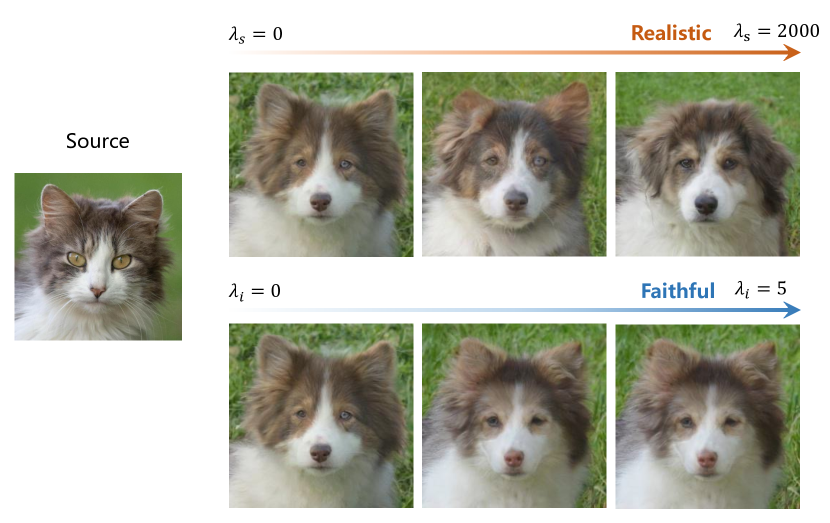
Figure 7: The qualitative results about the ablation of experts.

C.6 More Qualitative Results

In this section, we show more qualitative results on three unpaired I2I tasks using the default hyper-parameters in Figure  5. We also select some failure cases in Figure 6 and randomly selected qualitative results in Figure 8.

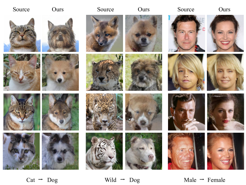
Figure 8: The randomly selected qualitative results with EGSDE.

C.7 Comparison with StarGAN v2

In this section, we compare the EGSDE with StarGAN v2[8] on the most popular benchmark $Cat\to Dog$. Since the FID measurement in CUT we mainly follow and StarGAN v2 is different, for fairness, we perform experiments under both FID metrics. The results are shown in Table 1 and Table 9. The qualitative comparisons are shown in Figure 9.

As shown in Table 1 and Table 9, the EGSDE outperforms StarGAN v2 in all metrics under the two different measurements. It also should be noted that the three faithful metrics for StarGAN v2 is much worse than ours. This is because the goal of StarGAN v2 is to generate diverse images over multi-domains, which pays little attention into the faithfulness. The qualitative comparisons in Figure 9 shows that StarGAN v2 loses much domain-independent features (e.g. background and color) while EGSDE can still retain them.

Table 9: The comparison with StarGAN v2[8] on Cat $\to$ Dog following the FID measurement of StarGAN v2. The EGSDE use the default-parameters ($\lambda_{s}=500,\lambda_{i}=2,M=0.5T$) and EGSDE^† use the parameters ($\lambda_{s}=700,\lambda_{i}=10,M=0.6T$).

Methods	FID$\downarrow$
StarGAN v2 [8]	36.37
EGSDE	48.20
EGSDE†	31.14

Figure 9: The qualitative comparisons with StarGAN v2. Each method generates five images by random seed for each source image. StarGAN v2 loses much domain-independent features (e.g. background and color) while EGSDE can still retain them.

Table 10: The results of replacing $E_{s}$ with classifier guidance on Cat $\to$ Dog.

Methods	FID$\downarrow$	L2$\downarrow$	PSNR$\uparrow$	SSIM $\uparrow$
EGSDE ($\lambda_{s}=500,\lambda_{i}=2$)	65.82	47.22	19.31	0.415
EGSDE-Classifier($\lambda_{s}=5,\lambda_{i}=2$ )	73.36	46.4	19.75	0.430
EGSDE-Classifier ($\lambda_{s}=50,\lambda_{i}=2$)	71.90	46.8	19.67	0.428
EGSDE-Classifier ($\lambda_{s}=500,\lambda_{i}=2$)	68.80	47.89	19.46	0.423

Table 11: The comparison with EGSDE-DDIM.

Methods	FID$\downarrow$	L2$\downarrow$	PSNR$\uparrow$	SSIM $\uparrow$
EGSDE-DDPM($\lambda_{s}=0,\lambda_{i}=0$)	74.17	47.88	19.19	0.423
EGSDE-DDPM($\lambda_{s}=500,\lambda_{i}=2$)	65.82	47.22	19.31	0.415
EGSDE-DDPM($\lambda_{s}=500,\lambda_{i}=0$)	62.44	51.02	18.64	0.405
EGSDE-DDPM($\lambda_{s}=0,\lambda_{i}=2$)	77.05	44.23	19.86	0.431
EGSDE-DDIM($\lambda_{s}=0,\lambda_{i}=0$)	88.29	41.93	20.62	0.472
EGSDE-DDIM($\lambda_{s}=500,\lambda_{i}=2$)	78.11	41.95	20.61	0.468
EGSDE-DDIM($\lambda_{s}=500,\lambda_{i}=0$)	74.32	44.32	20.12	0.460
EGSDE-DDIM($\lambda_{s}=0,\lambda_{i}=2$)	91.81	39.80	21.10	0.481

Table 12: Quantitative results in multi-domain translation, where the source domain includes Cat and Wild and the target domain is Dog. All experiments are repeated 5 times to eliminate randomness.

Methods	FID$\downarrow$	L2$\downarrow$	PSNR$\uparrow$	SSIM $\uparrow$
ILVR [7]	74.85 ± 1.24	60.16 ± 0.14	17.31 ± 0.02	0.325 ± 0.001
SDEdit [32]	71.34 ± 0.64	51.62 ± 0.05	18.58 ± 0.01	0.383 ± 0.001
EGSDE	64.02 ± 0.43	50.74 ± 0.04	18.73 ± 0.01	0.373 ± 0.000

Appendix D Multi-Domain Image Translation

Following [7], we extend our method into multi-domain translation on AFHQ dataset, where the source domain includes Cat and Wild and the target domain is Dog. In this setting, similar to two-domain unpaired I2I, the EGSDE also employs an energy function pretrained on both the source and target domains to guide the inference process of a pretrained SDE. The only difference is the domain-specific feature extractor $E_{s}(·,·)$ involved in the energy function is the all but the last layer of a three-class classifier rather than two-class. All experiments are repeated 5 times to eliminate randomness. The quantitative results are reported in Table 12. We can observe that the EGSDE outperforms the baselines in almost all realism and faithfulness metrics, showing the great generalization of our method.

References

- [1] Matthew Amodio and Smita Krishnaswamy. Travelgan: Image-to-image translation by transformation vector learning. In Proceedings of the IEEE/CVF Conference on Computer Vision and Pattern Recognition, pages 8975–8984, 2019.
- [2] Fan Bao, Chongxuan Li, Jun Zhu, and Bo Zhang. Analytic-dpm: an analytic estimate of the optimal reverse variance in diffusion probabilistic models. In International Conference on Learning Representations, 2021.
- [3] Sagie Benaim and Lior Wolf. One-sided unsupervised domain mapping. Advances in Neural Information Processing Systems, 30, 2017.
- [4] Mikołaj Bińkowski, Danica J Sutherland, Michael Arbel, and Arthur Gretton. Demystifying mmd gans. In International Conference on Learning Representations, 2018.
- [5] Christopher M. Bishop. Pattern Recognition and Machine Learning. 2006.
- [6] Xi Chen, Yan Duan, Rein Houthooft, John Schulman, Ilya Sutskever, and Pieter Abbeel. Infogan: Interpretable representation learning by information maximizing generative adversarial nets. Advances in Neural Information Processing Systems, 29, 2016.
- [7] Jooyoung Choi, Sungwon Kim, Yonghyun Jeong, Youngjune Gwon, and Sungroh Yoon. Ilvr: Conditioning method for denoising diffusion probabilistic models. In Proceedings of the IEEE/CVF International Conference on Computer Vision, pages 14367–14376, 2021.
- [8] Yunjey Choi, Youngjung Uh, Jaejun Yoo, and Jung-Woo Ha. Stargan v2: Diverse image synthesis for multiple domains. In Proceedings of the IEEE/CVF Conference on Computer Vision and Pattern Recognition, pages 8188–8197, 2020.
- [9] Prafulla Dhariwal and Alexander Nichol. Diffusion models beat gans on image synthesis. Advances in Neural Information Processing Systems, 34, 2021.
- [10] Huan Fu, Mingming Gong, Chaohui Wang, Kayhan Batmanghelich, Kun Zhang, and Dacheng Tao. Geometry-consistent generative adversarial networks for one-sided unsupervised domain mapping. In Proceedings of the IEEE/CVF Conference on Computer Vision and Pattern Recognition, pages 2427–2436, 2019.
- [11] Aaron Gokaslan, Vivek Ramanujan, Daniel Ritchie, Kwang In Kim, and James Tompkin. Improving shape deformation in unsupervised image-to-image translation. In Proceedings of the European Conference on Computer Vision, pages 649–665, 2018.
- [12] Ian Goodfellow, Jean Pouget-Abadie, Mehdi Mirza, Bing Xu, David Warde-Farley, Sherjil Ozair, Aaron Courville, and Yoshua Bengio. Generative adversarial nets. Advances in Neural Information Processing Systems, 27, 2014.
- [13] Martin Heusel, Hubert Ramsauer, Thomas Unterthiner, Bernhard Nessler, and Sepp Hochreiter. Gans trained by a two time-scale update rule converge to a local nash equilibrium. Advances in Neural Information Processing Systems, 30, 2017.
- [14] Irina Higgins, Loic Matthey, Arka Pal, Christopher Burgess, Xavier Glorot, Matthew Botvinick, Shakir Mohamed, and Alexander Lerchner. beta-vae: Learning basic visual concepts with a constrained variational framework. 2016.
- [15] Geoffrey E Hinton. Training products of experts by minimizing contrastive divergence. Neural computation, 14(8):1771–1800, 2002.
- [16] Jonathan Ho, Ajay Jain, and Pieter Abbeel. Denoising diffusion probabilistic models. Advances in Neural Information Processing Systems, 33:6840–6851, 2020.
- [17] Xun Huang, Ming-Yu Liu, Serge Belongie, and Jan Kautz. Multimodal unsupervised image-to-image translation. In Proceedings of the European Conference on Computer Vision, pages 172–189, 2018.
- [18] Phillip Isola, Jun-Yan Zhu, Tinghui Zhou, and Alexei A Efros. Image-to-image translation with conditional adversarial networks. In Proceedings of the IEEE conference on computer vision and pattern recognition, pages 1125–1134, 2017.
- [19] Liming Jiang, Changxu Zhang, Mingyang Huang, Chunxiao Liu, Jianping Shi, and Chen Change Loy. Tsit: A simple and versatile framework for image-to-image translation. In Proceedings of the European Conference on Computer Vision, pages 206–222, 2020.
- [20] Tero Karras, Timo Aila, Samuli Laine, and Jaakko Lehtinen. Progressive growing of gans for improved quality, stability, and variation. In International Conference on Learning Representations, 2018.
- [21] Oren Katzir, Dani Lischinski, and Daniel Cohen-Or. Cross-domain cascaded deep translation. In Proceedings of the European Conference on Computer Vision, pages 673–689, 2020.
- [22] Gwanghyun Kim, Taesung Kwon, and Jong Chul Ye. Diffusionclip: Text-guided diffusion models for robust image manipulation. In Proceedings of the IEEE/CVF Conference on Computer Vision and Pattern Recognition, pages 2426–2435, 2022.
- [23] Hyunjik Kim and Andriy Mnih. Disentangling by factorising. In International Conference on Machine Learning, pages 2649–2658, 2018.
- [24] Junho Kim, Minjae Kim, Hyeonwoo Kang, and Kwang Hee Lee. U-gat-it: Unsupervised generative attentional networks with adaptive layer-instance normalization for image-to-image translation. In International Conference on Learning Representations, 2019.
- [25] Taeksoo Kim, Moonsu Cha, Hyunsoo Kim, Jung Kwon Lee, and Jiwon Kim. Learning to discover cross-domain relations with generative adversarial networks. In International Conference on Machine Learning, pages 1857–1865, 2017.
- [26] Hsin-Ying Lee, Hung-Yu Tseng, Jia-Bin Huang, Maneesh Singh, and Ming-Hsuan Yang. Diverse image-to-image translation via disentangled representations. In Proceedings of the European Conference on Computer Vision, pages 35–51, 2018.
- [27] Minjun Li, Haozhi Huang, Lin Ma, Wei Liu, Tong Zhang, and Yugang Jiang. Unsupervised image-to-image translation with stacked cycle-consistent adversarial networks. In Proceedings of the European Conference on Computer Vision, pages 184–199, 2018.
- [28] Alexander H Liu, Yen-Cheng Liu, Yu-Ying Yeh, and Yu-Chiang Frank Wang. A unified feature disentangler for multi-domain image translation and manipulation. Advances in Neural Information Processing Systems, 31, 2018.
- [29] Ming-Yu Liu, Thomas Breuel, and Jan Kautz. Unsupervised image-to-image translation networks. Advances in Neural Information Processing Systems, 30, 2017.
- [30] Xihui Liu, Dong Huk Park, Samaneh Azadi, Gong Zhang, Arman Chopikyan, Yuxiao Hu, Humphrey Shi, Anna Rohrbach, and Trevor Darrell. More control for free! image synthesis with semantic diffusion guidance. arXiv preprint arXiv:2112.05744, 2021.
- [31] Cheng Lu, Yuhao Zhou, Fan Bao, Jianfei Chen, Chongxuan Li, and Jun Zhu. Dpm-solver: A fast ode solver for diffusion probabilistic model sampling in around 10 steps. arXiv preprint arXiv:2206.00927, 2022.
- [32] Chenlin Meng, Yutong He, Yang Song, Jiaming Song, Jiajun Wu, Jun-Yan Zhu, and Stefano Ermon. Sdedit: Guided image synthesis and editing with stochastic differential equations. In International Conference on Learning Representations, 2021.
- [33] Alex Nichol, Prafulla Dhariwal, Aditya Ramesh, Pranav Shyam, Pamela Mishkin, Bob McGrew, Ilya Sutskever, and Mark Chen. Glide: Towards photorealistic image generation and editing with text-guided diffusion models. arXiv preprint arXiv:2112.10741, 2021.
- [34] Alexander Quinn Nichol and Prafulla Dhariwal. Improved denoising diffusion probabilistic models. In International Conference on Machine Learning, pages 8162–8171, 2021.
- [35] Yingxue Pang, Jianxin Lin, Tao Qin, and Zhibo Chen. Image-to-image translation: Methods and applications. IEEE Transactions on Multimedia, 2021.
- [36] Taesung Park, Alexei A Efros, Richard Zhang, and Jun-Yan Zhu. Contrastive learning for unpaired image-to-image translation. In Proceedings of the European Conference on Computer Vision, pages 319–345, 2020.
- [37] Taesung Park, Ming-Yu Liu, Ting-Chun Wang, and Jun-Yan Zhu. Semantic image synthesis with spatially-adaptive normalization. In Proceedings of the IEEE/CVF Conference on Computer Vision and Pattern Recognition, pages 2337–2346, 2019.
- [38] Taesung Park, Jun-Yan Zhu, Oliver Wang, Jingwan Lu, Eli Shechtman, Alexei Efros, and Richard Zhang. Swapping autoencoder for deep image manipulation. Advances in Neural Information Processing Systems, 33:7198–7211, 2020.
- [39] Alec Radford, Jong Wook Kim, Chris Hallacy, Aditya Ramesh, Gabriel Goh, Sandhini Agarwal, Girish Sastry, Amanda Askell, Pamela Mishkin, Jack Clark, et al. Learning transferable visual models from natural language supervision. In International Conference on Machine Learning, pages 8748–8763, 2021.
- [40] Chitwan Saharia, William Chan, Huiwen Chang, Chris Lee, Jonathan Ho, Tim Salimans, David Fleet, and Mohammad Norouzi. Palette: Image-to-image diffusion models. In ACM SIGGRAPH, pages 1–10, 2022.
- [41] Chitwan Saharia, Jonathan Ho, William Chan, Tim Salimans, David J Fleet, and Mohammad Norouzi. Image super-resolution via iterative refinement. IEEE Transactions on Pattern Analysis and Machine Intelligence, 2022.
- [42] Eduardo Hugo Sanchez, Mathieu Serrurier, and Mathias Ortner. Learning disentangled representations via mutual information estimation. In Proceedings of the European Conference on Computer Vision, pages 205–221, 2020.
- [43] Hiroshi Sasaki, Chris G Willcocks, and Toby P Breckon. Unit-ddpm: Unpaired image translation with denoising diffusion probabilistic models. arXiv preprint arXiv:2104.05358, 2021.
- [44] Zhiqiang Shen, Mingyang Huang, Jianping Shi, Xiangyang Xue, and Thomas S Huang. Towards instance-level image-to-image translation. In Proceedings of the IEEE/CVF Conference on Computer Vision and Pattern Recognition, pages 3683–3692, 2019.
- [45] Assaf Shocher. Resizeright. https://github.com/assafshocher/ResizeRight, 2018.
- [46] Jascha Sohl-Dickstein, Eric Weiss, Niru Maheswaranathan, and Surya Ganguli. Deep unsupervised learning using nonequilibrium thermodynamics. In International Conference on Machine Learning, pages 2256–2265, 2015.
- [47] Jiaming Song, Chenlin Meng, and Stefano Ermon. Denoising diffusion implicit models. In International Conference on Learning Representations, 2020.
- [48] Yang Song, Conor Durkan, Iain Murray, and Stefano Ermon. Maximum likelihood training of score-based diffusion models. Advances in Neural Information Processing Systems, 34, 2021.
- [49] Yang Song and Stefano Ermon. Generative modeling by estimating gradients of the data distribution. Advances in Neural Information Processing Systems, 32, 2019.
- [50] Yang Song, Jascha Sohl-Dickstein, Diederik P Kingma, Abhishek Kumar, Stefano Ermon, and Ben Poole. Score-based generative modeling through stochastic differential equations. In International Conference on Learning Representations, 2020.
- [51] Hao Tang, Dan Xu, Nicu Sebe, Yanzhi Wang, Jason J Corso, and Yan Yan. Multi-channel attention selection gan with cascaded semantic guidance for cross-view image translation. In Proceedings of the IEEE/CVF Conference on Computer Vision and Pattern Recognition, pages 2417–2426, 2019.
- [52] Ting-Chun Wang, Ming-Yu Liu, Jun-Yan Zhu, Andrew Tao, Jan Kautz, and Bryan Catanzaro. High-resolution image synthesis and semantic manipulation with conditional gans. In Proceedings of the IEEE conference on computer vision and pattern recognition, pages 8798–8807, 2018.
- [53] Zhou Wang, Alan C Bovik, Hamid R Sheikh, and Eero P Simoncelli. Image quality assessment: from error visibility to structural similarity. IEEE Transactions on Image Processing, 13(4):600–612, 2004.
- [54] Wayne Wu, Kaidi Cao, Cheng Li, Chen Qian, and Chen Change Loy. Transgaga: Geometry-aware unsupervised image-to-image translation. In Proceedings of the IEEE/CVF Conference on Computer Vision and Pattern Recognition, pages 8012–8021, 2019.
- [55] Zili Yi, Hao Zhang, Ping Tan, and Minglun Gong. Dualgan: Unsupervised dual learning for image-to-image translation. In Proceedings of the IEEE International Conference on Computer Vision, pages 2849–2857, 2017.
- [56] Pan Zhang, Bo Zhang, Dong Chen, Lu Yuan, and Fang Wen. Cross-domain correspondence learning for exemplar-based image translation. In Proceedings of the IEEE/CVF Conference on Computer Vision and Pattern Recognition, pages 5143–5153, 2020.
- [57] Yihao Zhao, Ruihai Wu, and Hao Dong. Unpaired image-to-image translation using adversarial consistency loss. In Proceedings of the European Conference on Computer Vision, pages 800–815, 2020.
- [58] Chuanxia Zheng, Tat-Jen Cham, and Jianfei Cai. The spatially-correlative loss for various image translation tasks. In Proceedings of the IEEE/CVF Conference on Computer Vision and Pattern Recognition, pages 16407–16417, 2021.
- [59] Wanfeng Zheng, Qiang Li, Guoxin Zhang, Pengfei Wan, and Zhongyuan Wang. Ittr: Unpaired image-to-image translation with transformers. arXiv preprint arXiv:2203.16015, 2022.
- [60] Xingran Zhou, Bo Zhang, Ting Zhang, Pan Zhang, Jianmin Bao, Dong Chen, Zhongfei Zhang, and Fang Wen. Cocosnet v2: Full-resolution correspondence learning for image translation. In Proceedings of the IEEE/CVF Conference on Computer Vision and Pattern Recognition, pages 11465–11475, 2021.
- [61] Jun-Yan Zhu, Taesung Park, Phillip Isola, and Alexei A Efros. Unpaired image-to-image translation using cycle-consistent adversarial networks. In Proceedings of the IEEE International Conference on Computer Vision, pages 2223–2232, 2017.