Present Address: ]Simplex Holdings, Inc., 19F Toranomon Hills Mori Tower, 1-23-1 Toranomon, Minato-ku, Tokyo 105-6319, Japan; ishima.daisuke.m30@kyoto-u.ac.jp

Theory of rigidity and numerical analysis of density of states of two-dimensional amorphous solids with dispersed frictional grains in the linear response regime

Daisuke Ishima1 [ โ€ƒโ€ƒ Kuniyasu Saitoh2, Michio Otsuki3 and Hisao Hayakawa1 1Yukawa Institute for Theoretical Physics, Kyoto University,
Kitashirakawa-oiwake cho, Sakyo-ku, Kyoto 606-8502, Japan,
2Department of Physics, Faculty of Science, Kyoto Sangyo University,
Motoyama, Kamigamo, Kita-ku, Kyoto 603-8555, Japan,
3Graduate School of Engineering Science, Osaka University, Toyonaka, Osaka 560-8531, Japan
Abstract

Using the Jacobian matrix, we obtain theoretical expression of rigidity and the density of states of two-dimensional amorphous solids consisting of frictional grains in the linear response to an infinitesimal strain, in which we ignore the dynamical friction caused by the slip processes of contact points. The theoretical rigidity agrees with that obtained by molecular dynamics simulations. We confirm that the rigidity is smoothly connected to the value in the frictionless limit. For the density of states, we find that there are two modes in the density of states for sufficiently small kT/kNsubscript๐‘˜๐‘‡subscript๐‘˜๐‘k_{T}/k_{N}, which is the ratio of the tangential to normal stiffness. Rotational modes exist at low frequencies or small eigenvalues, whereas translational modes exist at high frequencies or large eigenvalues. The location of the rotational band shifts to the high-frequency region with an increase in kT/kNsubscript๐‘˜๐‘‡subscript๐‘˜๐‘k_{T}/k_{N} and becomes indistinguishable from the translational band for large kT/kNsubscript๐‘˜๐‘‡subscript๐‘˜๐‘k_{T}/k_{N}.

I Introduction

Amorphous materials consisting of dispersed grains such as powders, colloids, bubbles, and emulsions are ubiquitous in nature Jaeger96 ; Durian95 ; Wyart05 ; Baule18 . These materials behave like liquids at low densities and exhibit solid-like mechanical responses above their jamming point Liu98 . In systems consisting of frictionless grains, the rigidity changes continuously, but the coordination number of grains changes discontinuously at the jamming point as a function of density Durian95 ; Wyart05 ; Hern03 . The critical behavior near the jamming point is of interest to physicists as a non-equilibrium phase transition Hern01 ; Trappe01 ; Zhang05 ; Majmudar07 ; Ciamarra11 . Dispersed grains above the jamming point are fragile and exhibit softening and yielding transition under certain loads Nagamanasa14 ; Knowlton14 ; Kawasaki16 ; Leishangthem17 ; Bohy17 ; Ozawa18 ; Clark18 ; Boschan19 ; Singh20 ; Otsuki21 .

For amorphous solids consisting of frictionless grains, it is useful to analyze the dynamical matrix or the Hessian matrix, which is defined as the second derivative of the potential of a collection of grains with respect to the displacements from their stable configuration Wyart05 ; WyarLettt05 ; Ellenbroek06 ; Lerner16 ; Gartner16 ; Bonfanti19 ; Baule18 . For instance, the rigidity can be determined by eigenvalues and eigenvectors DeGiuli14 ; Mizuno16 ; Maloney04 ; Maloney06 ; Lemaitre06 ; Zaccone11 . It has been reported that the minimum nonzero eigenvalue of the Hessian matrix decreases with increasing strain and eventually becomes negative, where an irreversible stress drop takes placeย Maloney04 ; Maloney06 ; Manning11 ; Dasgupta12 ; Ebrahem20 .

It is known that amorphous solids have characteristic properties at low temperatures (e.g., thermal conductivity and specific heat) that are quite different from those of crystalline solids since a long-time ago Zeller71 . These days, we have recognized that amorphous solids consisting of dispersed grains exhibit unique elastic-plastic behavior as a mechanical response to an applied strainย Nicolas18 . Because these properties are related to the density of states (DOS), there have been lots of studies on the DOS Hern03 ; Schirmacher07 ; Lerner16 ; Mizuno17 ; Wang19 . The DOS for systems composed of anisotropic grains, such as ellipses, dimers, deformable grains, and grains with rough surfaces, have been studied with the aid of the Hessian matrix Zeravcic09 ; Mailman09 ; Schreck10 ; Yunker11 ; Schreck12 ; Shiraishi19 ; Papanikolaou13 ; Britoa18 ; Treado21 ; Ikeda20 ; Ikeda21 . Because of the rotation of such anisotropic grains, there exists a rotational band in the DOS that is distinguishable from the translational band Mailman09 ; Yunker11 ; Schreck12 ; Britoa18 ; Ikeda20 ; Ikeda21 .

Even for systems of spherical grains that cannot be free from inter-particle friction, similar results are expected as a result of grain rotations. However, few studies have reported the existence of rotational bands in the DOS. Because the frictional force between the grains depends on the contact history, it cannot be expressed as a conservative force. Therefore, stability analysis for frictional grains based on the Hessian cannot be used. Nevertheless, the Hessian analysis using an effective potential for frictional grains has been performed Somfai07 ; Henkes10 . Recently, Liu et al. suggested that the Hessian analysis with another effective potential can be used even if slip processes exist Liu21 . The previous studies Somfai07 ; Henkes10 reported that friction between grains causes a continuous change in the functional form of the DOS from that of frictionless systems. However, there are only a few reports on whether an isolated band in the DOS originating from friction between grains is visible at lower frequencies.

Recently, Chattoraj et al. discussed the stability of the grain configuration under strain using the Jacobian matrix of frictional grains Chattoraj19 . They performed eigenvalue analysis under athermal quasi-static shear processes and determined the existence of oscillatory instability originating from inter-particle friction at a certain strain Chattoraj19 ; Chattoraj19E ; Charan20 . However, they did not discuss the rigidity or the DOS.

The theoretical determination of the rigidity of amorphous solids consisting of frictional grains is important for controlling amorphous solids. However, we do not know how to determine the rigidity from the Jacobian for the frictional grains.

The purpose of this study is to clarify the role of mutual friction between grains in terms of the rigidity and DOS. We focus on the response to an infinitesimal strain from a stable configuration of grains without any strain to obtain tangible results. In this study, we assume that there is no slip between grains because of an infinitesimal strain, and we then deal with friction as static friction.

The remainder of this paper is organized as follows. In the next section, we introduce the numerical method. In Sec. III, we introduce the Jacobian. Section IV consists of Sec IV.1, which deals with the theoretical prediction of rigidity in the linear response regime, and Sec. IV.2, which deals with the DOS. In the final section, we summarize the results of our study and discuss future work. The appendix consists of seven sections. In Appendix A, we summarize the method for preparing a stable grain configuration before applying shear. In Appendix B, we explain the implementation of the numerical integration method in the proposed system. In Appendix C, we summarize some properties of the Jacobian. In Appendix D, we present the explicit expressions of the Jacobian. In Appendix E, we investigate the effects of rattlers. In Appendix F, we write down the explicit results of Jacobian. In Appendix G, we derive the theoretical prediction of rigidity using the Jacobian. In Appendix H, we introduce the DOS using the Hessian analysis. In Appendix I, we investigate the system size dependence of the DOS. In Appendix J, we study the density dependence of the DOS.

II Numerical model

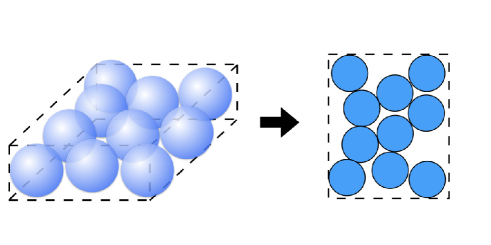
Our system contains N๐‘N frictional spherical particles embedded in a monolayer configuration. We treat this system as a two-dimensional system (see Fig. 1).
Refer to caption
Figure 1: Schematics of our system.

To prevent the system from crystallizing Luding01 , we prepare an equal number of particles with diameters d๐‘‘d and d/1.4๐‘‘1.4d/1.4. We assume that the mass of particle i๐‘–i is proportional to di2superscriptsubscript๐‘‘๐‘–2d_{i}^{2}, where disubscript๐‘‘๐‘–d_{i} is the diameter of i๐‘–i-th particle. We introduce m๐‘šm as the mass of a particle with diameter d๐‘‘d. In this study, xi,yisubscript๐‘ฅ๐‘–subscript๐‘ฆ๐‘–x_{i},y_{i}, and ฮธisubscript๐œƒ๐‘–\theta_{i} denote x,y๐‘ฅ๐‘ฆx,y coordinates, and the rotational angle of the i๐‘–i-th particle, respectively. We introduce the generalized coordinates of the i๐‘–i-th particle ๐’’i:=(๐’“iT,โ„“i)Tassignsubscript๐’’๐‘–superscriptsuperscriptsubscript๐’“๐‘–Tsubscriptโ„“๐‘–T\bm{q}_{i}:=(\bm{r}_{i}^{\textrm{T}},\ell_{i})^{\textrm{T}} with ๐’’i:=(xi,yi)Tassignsubscript๐’’๐‘–superscriptsubscript๐‘ฅ๐‘–subscript๐‘ฆ๐‘–T\bm{q}_{i}:=(x_{i},y_{i})^{\textrm{T}} and โ„“i:=diโ€‹ฮธi/2assignsubscriptโ„“๐‘–subscript๐‘‘๐‘–subscript๐œƒ๐‘–2\ell_{i}:=d_{i}\theta_{i}/2, where the superscript T denotes the transposition.

Let the force, and z๐‘งz-component of the torque acting on the i๐‘–i-th particle be ๐‘ญi:=(Fix,Fiy)Tassignsubscript๐‘ญ๐‘–superscriptsuperscriptsubscript๐น๐‘–๐‘ฅsuperscriptsubscript๐น๐‘–๐‘ฆT\bm{F}_{i}:=(F_{i}^{x},F_{i}^{y})^{\textrm{T}} and Tisubscript๐‘‡๐‘–T_{i}, respectively. Then, the equations of motion of i๐‘–i-th particle are expressed as

miโ€‹d2โ€‹๐’“idโ€‹t2subscript๐‘š๐‘–superscript๐‘‘2subscript๐’“๐‘–๐‘‘superscript๐‘ก2\displaystyle m_{i}\frac{d^{2}\bm{r}_{i}}{dt^{2}} =๐‘ญi,absentsubscript๐‘ญ๐‘–\displaystyle=\bm{F}_{i}, (1)
Iiโ€‹d2โ€‹ฮธidโ€‹t2subscript๐ผ๐‘–superscript๐‘‘2subscript๐œƒ๐‘–๐‘‘superscript๐‘ก2\displaystyle I_{i}\frac{d^{2}\theta_{i}}{dt^{2}} =Tiabsentsubscript๐‘‡๐‘–\displaystyle=T_{i} (2)

with the mass misubscript๐‘š๐‘–m_{i} and the momentum of inertia Ii:=miโ€‹di2/8assignsubscript๐ผ๐‘–subscript๐‘š๐‘–superscriptsubscript๐‘‘๐‘–28I_{i}:=m_{i}d_{i}^{2}/8 of i๐‘–i-th particle. In a system without volume forces such as gravity, we can write

๐‘ญisubscript๐‘ญ๐‘–\displaystyle\bm{F}_{i} =โˆ‘jโ‰ i๐’‡iโ€‹j,absentsubscript๐‘—๐‘–subscript๐’‡๐‘–๐‘—\displaystyle=\sum_{j\neq i}\bm{f}_{ij}, (3)
Tisubscript๐‘‡๐‘–\displaystyle T_{i} =โˆ‘jโ‰ iTiโ€‹j,absentsubscript๐‘—๐‘–subscript๐‘‡๐‘–๐‘—\displaystyle=\sum_{j\neq i}T_{ij}, (4)

where ๐’‡iโ€‹jsubscript๐’‡๐‘–๐‘—\bm{f}_{ij} and Tiโ€‹jsubscript๐‘‡๐‘–๐‘—T_{ij} are the force and z๐‘งz-component of the torque acting on the i๐‘–i-th particle from the j๐‘—j-th particle, respectively. Here, Tiโ€‹jsubscript๐‘‡๐‘–๐‘—T_{ij} is given by

Tiโ€‹j=โˆ’di2โ€‹(niโ€‹jxโ€‹fiโ€‹jyโˆ’niโ€‹jyโ€‹fiโ€‹jx),subscript๐‘‡๐‘–๐‘—subscript๐‘‘๐‘–2superscriptsubscript๐‘›๐‘–๐‘—๐‘ฅsuperscriptsubscript๐‘“๐‘–๐‘—๐‘ฆsuperscriptsubscript๐‘›๐‘–๐‘—๐‘ฆsuperscriptsubscript๐‘“๐‘–๐‘—๐‘ฅ\displaystyle T_{ij}=-\frac{d_{i}}{2}({n}_{ij}^{x}{f}_{ij}^{y}-{n}_{ij}^{y}{f}_{ij}^{x}), (5)

where we have introduced the normal unit vector between i๐‘–i and j๐‘—j particles as ๐’iโ€‹j:=๐’“iโ€‹j/|๐’“iโ€‹j|:=(๐’“iโˆ’๐’“j)/|๐’“iโˆ’๐’“j|assignsubscript๐’๐‘–๐‘—subscript๐’“๐‘–๐‘—subscript๐’“๐‘–๐‘—assignsubscript๐’“๐‘–subscript๐’“๐‘—subscript๐’“๐‘–subscript๐’“๐‘—\bm{n}_{ij}:=\bm{r}_{ij}/|\bm{r}_{ij}|:=(\bm{r}_{i}-\bm{r}_{j})/|\bm{r}_{i}-\bm{r}_{j}|. Here, niโ€‹jฮถsuperscriptsubscript๐‘›๐‘–๐‘—๐œn_{ij}^{\zeta} and fiโ€‹jฮถsuperscriptsubscript๐‘“๐‘–๐‘—๐œf_{ij}^{\zeta} refer to ฮถ๐œ\zeta-components of ๐’iโ€‹jsubscript๐’๐‘–๐‘—\bm{n}_{ij} and ๐’‡iโ€‹jsubscript๐’‡๐‘–๐‘—\bm{f}_{ij}, respectively. Note that ฮถ๐œ\zeta expresses ฮถ=x๐œ๐‘ฅ\zeta=x or y๐‘ฆy throughout this study. The force ๐’‡iโ€‹jsubscript๐’‡๐‘–๐‘—\bm{f}_{ij} can be divided into normal ๐’‡N,iโ€‹jsubscript๐’‡๐‘๐‘–๐‘—\bm{f}_{N,ij} and tangential ๐’‡T,iโ€‹jsubscript๐’‡๐‘‡๐‘–๐‘—\bm{f}_{T,ij} parts as

๐’‡iโ€‹j=(๐’‡N,iโ€‹j+๐’‡T,iโ€‹j)โ€‹ฮ˜โ€‹(diโ€‹j/2โˆ’|๐’“iโ€‹j|),subscript๐’‡๐‘–๐‘—subscript๐’‡๐‘๐‘–๐‘—subscript๐’‡๐‘‡๐‘–๐‘—ฮ˜subscript๐‘‘๐‘–๐‘—2subscript๐’“๐‘–๐‘—\displaystyle\bm{f}_{ij}=(\bm{f}_{N,ij}+\bm{f}_{T,ij})\Theta(d_{ij}/2-|\bm{r}_{ij}|), (6)

where diโ€‹j:=di+djassignsubscript๐‘‘๐‘–๐‘—subscript๐‘‘๐‘–subscript๐‘‘๐‘—d_{ij}:=d_{i}+d_{j} and ฮ˜โ€‹(x)ฮ˜๐‘ฅ\Theta(x) is Heavisideโ€™s step function, taking ฮ˜โ€‹(x)=1ฮ˜๐‘ฅ1\Theta(x)=1 for x>0๐‘ฅ0x>0 and ฮ˜โ€‹(x)=0ฮ˜๐‘ฅ0\Theta(x)=0 otherwise. We model the repulsive force between the contacted particles i๐‘–i and j๐‘—j as the Hertzian force in addition to the dissipative force proportional to the relative velocity with a damping constant ฮทDsubscript๐œ‚๐ท\eta_{D} Liu21 as follows:

๐’‡N,iโ€‹j::subscript๐’‡๐‘๐‘–๐‘—absent\displaystyle\bm{f}_{N,ij}: =kNโ€‹ฮพN,iโ€‹j3/2โ€‹๐’iโ€‹jโˆ’ฮทDโ€‹๐’—N,iโ€‹j,absentsubscript๐‘˜๐‘superscriptsubscript๐œ‰๐‘๐‘–๐‘—32subscript๐’๐‘–๐‘—subscript๐œ‚๐ทsubscript๐’—๐‘๐‘–๐‘—\displaystyle=k_{N}\xi_{N,ij}^{3/2}\bm{n}_{ij}-\eta_{D}\bm{v}_{N,ij}, (7)
๐’‡T,iโ€‹j::subscript๐’‡๐‘‡๐‘–๐‘—absent\displaystyle\bm{f}_{T,ij}: =kTโ€‹ฮพN,iโ€‹j1/2โ€‹ฮพT,iโ€‹jโ€‹๐’•iโ€‹jโˆ’ฮทDโ€‹๐’—T,iโ€‹j,absentsubscript๐‘˜๐‘‡superscriptsubscript๐œ‰๐‘๐‘–๐‘—12subscript๐œ‰๐‘‡๐‘–๐‘—subscript๐’•๐‘–๐‘—subscript๐œ‚๐ทsubscript๐’—๐‘‡๐‘–๐‘—\displaystyle=k_{T}\xi_{N,ij}^{1/2}\xi_{T,ij}\bm{t}_{ij}-\eta_{D}\bm{v}_{T,ij}, (8)

where kNsubscript๐‘˜๐‘k_{N} and kTsubscript๐‘˜๐‘‡k_{T} are the stiffness parameters of normal and tangential contacts, respectively. For the normal compression length and its velocity are denoted as ฮพN,iโ€‹j:=diโ€‹j/2โˆ’|๐’“iโ€‹j|assignsubscript๐œ‰๐‘๐‘–๐‘—subscript๐‘‘๐‘–๐‘—2subscript๐’“๐‘–๐‘—\xi_{N,ij}:=d_{ij}/2-|\bm{r}_{ij}| and ๐’—N,iโ€‹j:=(๐’“ห™iโ€‹jโ‹…๐’iโ€‹j)โ€‹๐’iโ€‹j,assignsubscript๐’—๐‘๐‘–๐‘—โ‹…subscriptห™๐’“๐‘–๐‘—subscript๐’๐‘–๐‘—subscript๐’๐‘–๐‘—\bm{v}_{N,ij}:=(\dot{\bm{r}}_{ij}\cdot\bm{n}_{ij})\bm{n}_{ij}, respectively. For the tangential deformation, with the aid of ๐’–iโ€‹j:=(niโ€‹jy,โˆ’niโ€‹jx)Tassignsubscript๐’–๐‘–๐‘—superscriptsuperscriptsubscript๐‘›๐‘–๐‘—๐‘ฆsuperscriptsubscript๐‘›๐‘–๐‘—๐‘ฅT\bm{u}_{ij}:=(n_{ij}^{y},-n_{ij}^{x})^{\textrm{T}}, the tangential velocity ๐’—T,iโ€‹jsubscript๐’—๐‘‡๐‘–๐‘—\bm{v}_{T,ij} is defined as ๐’—T,iโ€‹j:=๐’“ห™iโ€‹jโˆ’๐’—N,iโ€‹j+๐’–iโ€‹jโ€‹(diโ€‹ฯ‰i+djโ€‹ฯ‰j)/2assignsubscript๐’—๐‘‡๐‘–๐‘—subscriptห™๐’“๐‘–๐‘—subscript๐’—๐‘๐‘–๐‘—subscript๐’–๐‘–๐‘—subscript๐‘‘๐‘–subscript๐œ”๐‘–subscript๐‘‘๐‘—subscript๐œ”๐‘—2\bm{v}_{T,ij}:=\dot{\bm{r}}_{ij}-\bm{v}_{N,ij}+\bm{u}_{ij}(d_{i}\omega_{i}+d_{j}\omega_{j})/2, where we have introduced

๐ƒT,iโ€‹j:=โˆซCiโ€‹j๐‘‘tโ€‹๐’—T,iโ€‹jโˆ’[(โˆซCiโ€‹j๐‘‘tโ€‹๐’—T,iโ€‹j)โ‹…๐’iโ€‹j]โ€‹๐’iโ€‹j,assignsubscript๐ƒ๐‘‡๐‘–๐‘—subscriptsubscript๐ถ๐‘–๐‘—differential-d๐‘กsubscript๐’—๐‘‡๐‘–๐‘—delimited-[]โ‹…subscriptsubscript๐ถ๐‘–๐‘—differential-d๐‘กsubscript๐’—๐‘‡๐‘–๐‘—subscript๐’๐‘–๐‘—subscript๐’๐‘–๐‘—\displaystyle\bm{\xi}_{T,ij}:=\int_{C_{ij}}dt\bm{v}_{T,ij}-\left[\left(\int_{C_{ij}}dt\bm{v}_{T,ij}\right)\cdot\bm{n}_{ij}\right]\bm{n}_{ij}, (9)

with ฮพT,iโ€‹j:=|๐ƒT,iโ€‹j|assignsubscript๐œ‰๐‘‡๐‘–๐‘—subscript๐ƒ๐‘‡๐‘–๐‘—\xi_{T,ij}:=|\bm{\xi}_{T,ij}| and ๐’•iโ€‹j:=โˆ’๐ƒT,iโ€‹j/ฮพT,iโ€‹jassignsubscript๐’•๐‘–๐‘—subscript๐ƒ๐‘‡๐‘–๐‘—subscript๐œ‰๐‘‡๐‘–๐‘—\bm{t}_{ij}:=-\bm{\xi}_{T,ij}/\xi_{T,ij}. Here, ๐‘จห™:=dโ€‹๐‘จ/dโ€‹tassignห™๐‘จ๐‘‘๐‘จ๐‘‘๐‘ก\dot{\bm{A}}:=d\bm{A}/dt and โˆซCiโ€‹j๐‘‘tsubscriptsubscript๐ถ๐‘–๐‘—differential-d๐‘ก\int_{C_{ij}}dt is the integration over the duration time of contact between i๐‘–i and j๐‘—j particles. Although the dissipative force between grains interacting with the Hertzian force is proportional to the product of the relative velocity and ฮพN,iโ€‹j1/2superscriptsubscript๐œ‰๐‘๐‘–๐‘—12\xi_{N,ij}^{1/2} Kuwabara87 ; Brilliantov96 ; Morgado97 , we adopt simple dissipative forces as in Eqs. (7) and (8) because we are not interested in the relaxation dynamics. We note that Eqs. (7) and (8) assume the Hertzian contact force for the static repulsion of contacting spheres, but all calculations in this study are those for two-dimensional systems. Here, we do not consider the effects of slips in the tangential equation of motion. This treatment can be justified if we restrict our interest in the linear response regime to a stable configuration of particles without any strain. This situation corresponds to frictional grains with infinitely large dynamical friction constant, in which the friction is only characterized by static friction. Therefore, our analysis does not apply to systems with finite strain Otsuki17 , where the effect of slip is important.

To generate a stable configuration of frictional particles, we prepare a stable configuration of frictionless particles in a square box of linear size L๐ฟL using a fast inertial relaxation engine (FIRE) Bitzek06 . Subsequently, we turn on the tangential force using Eqs. (1) and (2) to achieve a stable configuration in the force-balanced (FB) state for frictional particle111 For simplicity, we prepare the configuration before applying shear for frictionless particles at first, and then considered the friction between particles. If we prepare a configuration before applying shear by compressing frictional particles, we confirm that the configuration had an oscillatory instability that resulted from the appearance of a pair of imaginary eigenvalues of the Jacobian divided by mass matrix: ฮปโ€ฒ=ฮปrโ€ฒยฑiโ€‹ฮปiโ€ฒsuperscript๐œ†โ€ฒplus-or-minussubscriptsuperscript๐œ†โ€ฒ๐‘Ÿ๐‘–subscriptsuperscript๐œ†โ€ฒ๐‘–\lambda^{\prime}=\lambda^{\prime}_{r}\pm i\lambda^{\prime}_{i} Chattoraj19 ; Chattoraj19E ; Charan20 , where ฮปโ€ฒ,ฮปrโ€ฒsuperscript๐œ†โ€ฒsubscriptsuperscript๐œ†โ€ฒ๐‘Ÿ\lambda^{\prime},\lambda^{\prime}_{r}, and ฮปiโ€ฒsubscriptsuperscript๐œ†โ€ฒ๐‘–\lambda^{\prime}_{i} are the complex, real, and imaginary eigenvalues of Mโˆ’1โ€‹๐’ฅsuperscript๐‘€1๐’ฅM^{-1}\mathcal{J}, respectively. Here, ๐’ฅ๐’ฅ\mathcal{J} is the Jacobian defined in Eq. (18), and M๐‘€M is the mass matrix whose explicit form is given by M=[M1โ‹ฑMN]๐‘€delimited-[]matrixsubscript๐‘€1missing-subexpressionmissing-subexpressionโ‹ฑmissing-subexpressionmissing-subexpressionsubscript๐‘€๐‘M=\left[\begin{matrix}M_{1}&\\ &\ddots\\ &&M_{N}\end{matrix}\right], where Mi:=[mimi4โ€‹Ii/di2]assignsubscript๐‘€๐‘–delimited-[]matrixsubscript๐‘š๐‘–missing-subexpressionmissing-subexpressionmissing-subexpressionsubscript๐‘š๐‘–missing-subexpressionmissing-subexpressionmissing-subexpression4subscript๐ผ๐‘–superscriptsubscript๐‘‘๐‘–2M_{i}:=\left[\begin{matrix}m_{i}&&\\ &m_{i}&\\ &&4I_{i}/d_{i}^{2}\end{matrix}\right]. Because the linearized equation of motion is expressed as d2โ€‹qiฮฑ/dโ€‹t2=โˆ’โˆ‘k,ฮบโˆ‘j,ฮฒ(Miโ€‹kฮฑโ€‹ฮบ)โˆ’1โ€‹๐’ฅkโ€‹jฮบโ€‹ฮฒโ€‹qjฮฒsuperscript๐‘‘2superscriptsubscript๐‘ž๐‘–๐›ผ๐‘‘superscript๐‘ก2subscript๐‘˜๐œ…subscript๐‘—๐›ฝsuperscriptsuperscriptsubscript๐‘€๐‘–๐‘˜๐›ผ๐œ…1superscriptsubscript๐’ฅ๐‘˜๐‘—๐œ…๐›ฝsuperscriptsubscript๐‘ž๐‘—๐›ฝd^{2}q_{i}^{\alpha}/dt^{2}=-\sum_{k,\kappa}\sum_{j,\beta}(M_{ik}^{\alpha\kappa})^{-1}\mathcal{J}_{kj}^{\kappa\beta}q_{j}^{\beta}, there are four fundamental solutions ๐’’โˆeiโ€‹ฯ‰nโ€ฒโ€‹tproportional-to๐’’superscript๐‘’๐‘–superscriptsubscript๐œ”๐‘›โ€ฒ๐‘ก\bm{q}\propto e^{i\omega_{n}^{\prime}t}, where iโ€‹ฯ‰nโ€ฒ๐‘–superscriptsubscript๐œ”๐‘›โ€ฒi\omega_{n}^{\prime} consists of iโ€‹ฯ‰ยฑ1โ€ฒ=ฯ‰iโ€ฒยฑiโ€‹ฯ‰rโ€ฒ๐‘–subscriptsuperscript๐œ”โ€ฒplus-or-minus1plus-or-minussubscriptsuperscript๐œ”โ€ฒ๐‘–๐‘–subscriptsuperscript๐œ”โ€ฒ๐‘Ÿi\omega^{\prime}_{\pm 1}=\omega^{\prime}_{i}\pm i\omega^{\prime}_{r} and iโ€‹ฯ‰ยฑ2โ€ฒ=โˆ’ฯ‰iโ€ฒยฑiโ€‹ฯ‰rโ€ฒ๐‘–subscriptsuperscript๐œ”โ€ฒplus-or-minus2plus-or-minussubscriptsuperscript๐œ”โ€ฒ๐‘–๐‘–subscriptsuperscript๐œ”โ€ฒ๐‘Ÿi\omega^{\prime}_{\pm 2}=-\omega^{\prime}_{i}\pm i\omega^{\prime}_{r}. Here, ฯ‰rโ€ฒsubscriptsuperscript๐œ”โ€ฒ๐‘Ÿ\omega^{\prime}_{r} and ฯ‰iโ€ฒsubscriptsuperscript๐œ”โ€ฒ๐‘–\omega^{\prime}_{i} satisfy the relation ฯ‰rโ€ฒยฑiโ€‹ฯ‰iโ€ฒ=ฮปrโ€ฒยฑiโ€‹ฮปiโ€ฒplus-or-minussubscriptsuperscript๐œ”โ€ฒ๐‘Ÿ๐‘–subscriptsuperscript๐œ”โ€ฒ๐‘–plus-or-minussubscriptsuperscript๐œ†โ€ฒ๐‘Ÿ๐‘–subscriptsuperscript๐œ†โ€ฒ๐‘–\omega^{\prime}_{r}\pm i\omega^{\prime}_{i}=\sqrt{\lambda^{\prime}_{r}\pm i\lambda^{\prime}_{i}}. Thus, to avoid the oscillatory instability of the configuration before applying shear, we adopt the protocol of creating the configuration with frictionless particles, and then let the system relax by adding static friction between particles. (see Appendix A for details). Here, the FB state satisfies the FB conditions |Fiฮถ|=0superscriptsubscript๐น๐‘–๐œ0|F_{i}^{\zeta}|=0 and |Ti|=0subscript๐‘‡๐‘–0|T_{i}|=0 for arbitrary particles. Note that we set ฮธi=0subscript๐œƒ๐‘–0\theta_{i}=0 when the tangential force is turned on.

We impose the Lees-Edwards boundary condition Lees72 ; Evans08 , where the direction parallel to the shear strain is x๐‘ฅx-direction. After applying a step strain ฮ”โ€‹ฮณฮ”๐›พ\Delta\gamma to all particles, x๐‘ฅx-coordinate of the position of the i๐‘–i-th particle is shifted by an affine displacement ฮ”โ€‹xiโ€‹(ฮ”โ€‹ฮณ):=ฮ”โ€‹ฮณโ€‹yiFBโ€‹(0)assignฮ”subscript๐‘ฅ๐‘–ฮ”๐›พฮ”๐›พsuperscriptsubscript๐‘ฆ๐‘–FB0\Delta x_{i}(\Delta\gamma):=\Delta\gamma y_{i}^{\textrm{FB}}(0), where the superscript FB denotes the FB state. The system is then relaxed to the FB state by the contact forces between the particles expressed in Eqs. (7) and (8). Here, ฮถ๐œ\zeta-components of translational ฮ”โ€‹rฬŠiฮถโ€‹(ฮ”โ€‹ฮณ)ฮ”superscriptsubscriptฬŠ๐‘Ÿ๐‘–๐œฮ”๐›พ\Delta\mathring{r}_{i}^{\zeta}(\Delta\gamma) and rotational ฮ”โ€‹โ„“ฬŠiโ€‹(ฮ”โ€‹ฮณ)ฮ”subscriptฬŠโ„“๐‘–ฮ”๐›พ\Delta\mathring{\ell}_{i}(\Delta\gamma) nonaffine displacements of the i๐‘–i-th particle after the relaxation process are, respectively, defined as

ฮ”โ€‹rฬŠiฮถโ€‹(ฮ”โ€‹ฮณ)::ฮ”superscriptsubscriptฬŠ๐‘Ÿ๐‘–๐œฮ”๐›พabsent\displaystyle\Delta\mathring{r}_{i}^{\zeta}(\Delta\gamma): =riFB,ฮถโ€‹(ฮ”โ€‹ฮณ)โˆ’riFB,ฮถโ€‹(0)โˆ’ฮดฮถโ€‹xโ€‹ฮ”โ€‹ฮณโ€‹yiFBโ€‹(0),absentsuperscriptsubscript๐‘Ÿ๐‘–FB๐œฮ”๐›พsuperscriptsubscript๐‘Ÿ๐‘–FB๐œ0subscript๐›ฟ๐œ๐‘ฅฮ”๐›พsuperscriptsubscript๐‘ฆ๐‘–FB0\displaystyle=r_{i}^{\textrm{FB},\zeta}(\Delta\gamma)-r_{i}^{\textrm{FB},\zeta}(0)-\delta_{\zeta x}\Delta\gamma y_{i}^{\textrm{FB}}(0), (10)
ฮ”โ€‹โ„“ฬŠi::ฮ”subscriptฬŠโ„“๐‘–absent\displaystyle\Delta\mathring{\ell}_{i}: =โ„“iFBโ€‹(ฮ”โ€‹ฮณ)โˆ’โ„“iFBโ€‹(0).absentsuperscriptsubscriptโ„“๐‘–FBฮ”๐›พsuperscriptsubscriptโ„“๐‘–FB0\displaystyle=\ell_{i}^{\textrm{FB}}(\Delta\gamma)-\ell_{i}^{\textrm{FB}}(0). (11)

Using Eqs. (10) and (11), we introduce the rate of nonaffine displacements as:

dโ€‹rฬŠiฮถdโ€‹ฮณ::๐‘‘superscriptsubscriptฬŠ๐‘Ÿ๐‘–๐œ๐‘‘๐›พabsent\displaystyle\frac{d\mathring{r}_{i}^{\zeta}}{d\gamma}: =limฮ”โ€‹ฮณโ†’0ฮ”โ€‹rฬŠiฮถโ€‹(ฮ”โ€‹ฮณ)ฮ”โ€‹ฮณabsentsubscriptโ†’ฮ”๐›พ0ฮ”superscriptsubscriptฬŠ๐‘Ÿ๐‘–๐œฮ”๐›พฮ”๐›พ\displaystyle=\lim_{\Delta\gamma\to 0}\frac{\Delta\mathring{r}_{i}^{\zeta}(\Delta\gamma)}{\Delta\gamma}
=limฮ”โ€‹ฮณโ†’0riFB,ฮถโ€‹(ฮ”โ€‹ฮณ)โˆ’riFB,ฮถโ€‹(0)ฮ”โ€‹ฮณโˆ’ฮดฮถโ€‹xโ€‹yiFBโ€‹(0),absentsubscriptโ†’ฮ”๐›พ0superscriptsubscript๐‘Ÿ๐‘–FB๐œฮ”๐›พsuperscriptsubscript๐‘Ÿ๐‘–FB๐œ0ฮ”๐›พsubscript๐›ฟ๐œ๐‘ฅsuperscriptsubscript๐‘ฆ๐‘–FB0\displaystyle=\lim_{\Delta\gamma\to 0}\frac{r_{i}^{\textrm{FB},\zeta}(\Delta\gamma)-r_{i}^{\textrm{FB},\zeta}(0)}{\Delta\gamma}-\delta_{\zeta x}y_{i}^{\textrm{FB}}(0), (12)
dโ€‹โ„“ฬŠidโ€‹ฮณ::๐‘‘subscriptฬŠโ„“๐‘–๐‘‘๐›พabsent\displaystyle\frac{d\mathring{\ell}_{i}}{d\gamma}: =limฮ”โ€‹ฮณโ†’0ฮ”โ€‹โ„“ฬŠiโ€‹(ฮ”โ€‹ฮณ)ฮ”โ€‹ฮณabsentsubscriptโ†’ฮ”๐›พ0ฮ”subscriptฬŠโ„“๐‘–ฮ”๐›พฮ”๐›พ\displaystyle=\lim_{\Delta\gamma\to 0}\frac{\Delta\mathring{\ell}_{i}(\Delta\gamma)}{\Delta\gamma}
=limฮ”โ€‹ฮณโ†’0โ„“iFBโ€‹(ฮ”โ€‹ฮณ)โˆ’โ„“iFBโ€‹(0)ฮ”โ€‹ฮณ.absentsubscriptโ†’ฮ”๐›พ0superscriptsubscriptโ„“๐‘–FBฮ”๐›พsuperscriptsubscriptโ„“๐‘–FB0ฮ”๐›พ\displaystyle=\lim_{\Delta\gamma\to 0}\frac{\ell_{i}^{\textrm{FB}}(\Delta\gamma)-\ell_{i}^{\textrm{FB}}(0)}{\Delta\gamma}. (13)

Our system is characterized by the generalized coordinate ๐’’โ€‹(ฮณ):=(๐’’1Tโ€‹(ฮณ),๐’’2Tโ€‹(ฮณ),โ‹ฏ,๐’’NTโ€‹(ฮณ))Tassign๐’’๐›พsuperscriptsuperscriptsubscript๐’’1T๐›พsuperscriptsubscript๐’’2T๐›พโ‹ฏsuperscriptsubscript๐’’๐‘T๐›พT\bm{q}(\gamma):=(\bm{q}_{1}^{\textrm{T}}(\gamma),\bm{q}_{2}^{\textrm{T}}(\gamma),\cdots,\bm{q}_{N}^{\textrm{T}}(\gamma))^{\textrm{T}}. The configuration in the FB state at strain ฮณ๐›พ\gamma is denoted as ๐’’FBโ€‹(ฮณ):=((๐’’1FBโ€‹(ฮณ))T,(๐’’2FBโ€‹(ฮณ))T,โ‹ฏ,(๐’’NFBโ€‹(ฮณ))T)Tassignsuperscript๐’’FB๐›พsuperscriptsuperscriptsuperscriptsubscript๐’’1FB๐›พTsuperscriptsuperscriptsubscript๐’’2FB๐›พTโ‹ฏsuperscriptsuperscriptsubscript๐’’๐‘FB๐›พTT\bm{q}^{\textrm{FB}}(\gamma):=((\bm{q}_{1}^{\textrm{FB}}(\gamma))^{\textrm{T}},(\bm{q}_{2}^{\textrm{FB}}(\gamma))^{\textrm{T}},\cdots,(\bm{q}_{N}^{\textrm{FB}}(\gamma))^{\textrm{T}})^{\textrm{T}}. The shear stress ฯƒxโ€‹yโ€‹(ฮณ)subscript๐œŽ๐‘ฅ๐‘ฆ๐›พ\sigma_{xy}(\gamma) at ๐’’FBโ€‹(ฮณ)superscript๐’’FB๐›พ\bm{q}^{\textrm{FB}}(\gamma) for one sample is given by:

ฯƒxโ€‹yโ€‹(๐’’FBโ€‹(ฮณ))=โˆ’1L2โ€‹โˆ‘iโˆ‘j>ifiโ€‹jxโ€‹(๐’’FBโ€‹(ฮณ))โ€‹riโ€‹jyโ€‹(๐’’FBโ€‹(ฮณ)).subscript๐œŽ๐‘ฅ๐‘ฆsuperscript๐’’FB๐›พ1superscript๐ฟ2subscript๐‘–subscript๐‘—๐‘–superscriptsubscript๐‘“๐‘–๐‘—๐‘ฅsuperscript๐’’FB๐›พsuperscriptsubscript๐‘Ÿ๐‘–๐‘—๐‘ฆsuperscript๐’’FB๐›พ\displaystyle\sigma_{xy}(\bm{q}^{\textrm{FB}}(\gamma))=-\frac{1}{L^{2}}\sum_{i}\sum_{j>i}f_{ij}^{x}(\bm{q}^{\textrm{FB}}(\gamma))r_{ij}^{y}(\bm{q}^{\textrm{FB}}(\gamma)). (14)

The rigidity g๐‘”g in the linear response regime for one sample is defined as

g๐‘”\displaystyle g :=dโ€‹ฯƒxโ€‹yโ€‹(๐’’โ€‹(ฮณ))dโ€‹ฮณ|๐’’โ€‹(ฮณ)=๐’’FBโ€‹(0),assignabsentevaluated-at๐‘‘subscript๐œŽ๐‘ฅ๐‘ฆ๐’’๐›พ๐‘‘๐›พ๐’’๐›พsuperscript๐’’FB0\displaystyle:=\left.\frac{d\sigma_{xy}(\bm{q}(\gamma))}{d\gamma}\right|_{\bm{q}(\gamma)=\bm{q}^{\textrm{FB}}(0)}, (15)

where the differentiation on the right-hand side (RHS) of Eq. (15) is defined as follows:

dโ€‹ฯƒxโ€‹yโ€‹(๐’’โ€‹(ฮณ))dโ€‹ฮณ|๐’’โ€‹(ฮณ)=๐’’FBโ€‹(0)evaluated-at๐‘‘subscript๐œŽ๐‘ฅ๐‘ฆ๐’’๐›พ๐‘‘๐›พ๐’’๐›พsuperscript๐’’FB0\displaystyle\left.\frac{d\sigma_{xy}(\bm{q}(\gamma))}{d\gamma}\right|_{\bm{q}(\gamma)=\bm{q}^{\textrm{FB}}(0)}
:=limฮ”โ€‹ฮณโ†’0ฯƒxโ€‹yโ€‹(๐’’FBโ€‹(ฮ”โ€‹ฮณ))โˆ’ฯƒxโ€‹yโ€‹(๐’’FBโ€‹(0))ฮ”โ€‹ฮณ.assignabsentsubscriptโ†’ฮ”๐›พ0subscript๐œŽ๐‘ฅ๐‘ฆsuperscript๐’’FBฮ”๐›พsubscript๐œŽ๐‘ฅ๐‘ฆsuperscript๐’’FB0ฮ”๐›พ\displaystyle\quad\quad\quad:=\lim_{\Delta\gamma\to 0}\frac{\sigma_{xy}(\bm{q}^{\textrm{FB}}(\Delta\gamma))-\sigma_{xy}(\bm{q}^{\textrm{FB}}(0))}{\Delta\gamma}. (16)

In the numerical calculation, we use a non-zero but sufficiently small ฮ”โ€‹ฮณฮ”๐›พ\Delta\gamma for the evaluation of g๐‘”g. Then, the rigidity G๐บG in the linear response regime is defined as

G๐บ\displaystyle G :=โŸจgโŸฉ,assignabsentexpectation๐‘”\displaystyle:=\Braket{g}, (17)

where โŸจโ‹…โŸฉdelimited-โŸจโŸฉโ‹…\langle\cdot\rangle is the ensemble average.

For the numerical FB condition, we use the condition |F~iฮฑ|<FThsuperscriptsubscript~๐น๐‘–๐›ผsubscript๐นTh|\tilde{F}_{i}^{\alpha}|<F_{\textrm{Th}} for arbitrary i๐‘–i, where FThsubscript๐นThF_{\textrm{Th}} is the threshold force for the simulation and ๐‘ญ~isubscript~๐‘ญ๐‘–\tilde{\bm{F}}_{i} is the generalized force, defined as ๐‘ญ~i:=(F~ix,F~iy,F~iโ„“)T:=(Fix,Fiy,2โ€‹Ti/di)Tassignsubscript~๐‘ญ๐‘–superscriptsuperscriptsubscript~๐น๐‘–๐‘ฅsuperscriptsubscript~๐น๐‘–๐‘ฆsuperscriptsubscript~๐น๐‘–โ„“Tassignsuperscriptsuperscriptsubscript๐น๐‘–๐‘ฅsuperscriptsubscript๐น๐‘–๐‘ฆ2subscript๐‘‡๐‘–subscript๐‘‘๐‘–T\tilde{\bm{F}}_{i}:=(\tilde{F}_{i}^{x},\tilde{F}_{i}^{y},\tilde{F}_{i}^{\ell})^{\textrm{T}}:=(F_{i}^{x},F_{i}^{y},2T_{i}/d_{i})^{\textrm{T}}.

In our simulation, we adopt ฮทD=(mโ€‹kN)1/2โ€‹d1/4subscript๐œ‚๐ทsuperscript๐‘šsubscript๐‘˜๐‘12superscript๐‘‘14\eta_{D}=(mk_{N})^{1/2}d^{1/4} and FTh=1.0ร—10โˆ’14โ€‹kNโ€‹d3/2subscript๐นTh1.0superscript1014subscript๐‘˜๐‘superscript๐‘‘32F_{\textrm{Th}}=1.0\times 10^{-14}k_{N}d^{3/2}. The control parameters are the ratio of the tangential to normal stiffness kT/kNsubscript๐‘˜๐‘‡subscript๐‘˜๐‘k_{T}/k_{N} and projected area fraction to two-dimensional space ฯ•italic-ฯ•\phi. The operating ranges of kT/kNsubscript๐‘˜๐‘‡subscript๐‘˜๐‘k_{T}/k_{N} and ฯ•italic-ฯ•\phi are 0.00.00.0 to 10.010.010.0 and 0.830.830.83 to 0.900.900.90, respectively. In this study, we mainly present the results for N=4096๐‘4096N=4096 and ฮ”โ€‹ฮณ=1.0ร—10โˆ’6ฮ”๐›พ1.0superscript106\Delta\gamma=1.0\times 10^{-6} with the ensemble averages of 101010 samples for each kT/kNsubscript๐‘˜๐‘‡subscript๐‘˜๐‘k_{T}/k_{N} and ฯ•italic-ฯ•\phi. Some results are obtained with N=1024๐‘1024N=1024, ฮ”โ€‹ฮณ=1.0ร—10โˆ’6ฮ”๐›พ1.0superscript106\Delta\gamma=1.0\times 10^{-6}, and five samples for each kT/kNsubscript๐‘˜๐‘‡subscript๐‘˜๐‘k_{T}/k_{N} and ฯ•italic-ฯ•\phi. We verify that the results are independent of the choice of ฮ”โ€‹ฮณฮ”๐›พ\Delta\gamma for 1.0ร—10โˆ’6โ‰คฮ”โ€‹ฮณโ‰ค1.0ร—10โˆ’41.0superscript106ฮ”๐›พ1.0superscript1041.0\times 10^{-6}\leq\Delta\gamma\leq 1.0\times 10^{-4}. We ignore the effect of dissipation between particles because the velocity of each particle is sufficiently small for infinitesimal agitation from the FB state. The time step of the simulation, ฮ”โ€‹tฮ”๐‘ก\Delta t, was set to ฮ”โ€‹t=1.0ร—10โˆ’2โ€‹t0ฮ”๐‘ก1.0superscript102subscript๐‘ก0\Delta t=1.0\times 10^{-2}t_{0}, and numerical integration was performed using the velocity Verlet method (see Appendix B), where t0:=(m/kN)1/2โ€‹d1/4assignsubscript๐‘ก0superscript๐‘šsubscript๐‘˜๐‘12superscript๐‘‘14t_{0}:=(m/k_{N})^{1/2}d^{1/4}. To obtain eigenvalues and eigenvectors of the Jacobian matrix, which will be introduced in detail in the next section, we have used the LAPACK, which provides a template library for linear algebra.

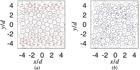
Figure 2 (a) shows an example of the affine displacements of particles, where the displacements exist only in the shear direction, and Fig. 2 (b) shows the nonaffine displacements.
Refer to caption
Figure 2: Plots of (a) affine displacements and (b) nonaffine displacements of particles with ฮ”โ€‹ฮณ=1.0ร—10โˆ’6ฮ”๐›พ1.0superscript106\Delta\gamma=1.0\times 10^{-6}. Here, the magnitudes of the vectors are multiplied by (a) 0.1โ€‹ฮ”โ€‹ฮณโˆ’10.1ฮ”superscript๐›พ10.1\Delta\gamma^{-1} and (b) 1.31.31.3 for the visualization. These figures are based on numerical results for N=128๐‘128N=128.

III Theoretical Analysis

In this section, we introduce the Jacobian, the DOS, and theoretical expressions of the linear rigidity. Here, we omit the effects of ๐’’ห™ห™๐’’\dot{\bm{q}} because the dissipative term proportional to ๐’’ห™ห™๐’’\dot{\bm{q}} vanishes under quasistatic shear.

III.1 Jacobian and the DOS for frictional particles

In frictional systems, the stability of the system and DOS at ๐’’FBโ€‹(ฮณ)superscript๐’’FB๐›พ\bm{q}^{\textrm{FB}}(\gamma) are analyzed using the Jacobian (๐’ฅ๐’ฅ\mathcal{J}) defined as Chattoraj19 :

๐’ฅiโ€‹jฮฑโ€‹ฮฒ:=โˆ’โˆ‚F~iฮฑโ€‹(๐’’โ€‹(ฮณ))โˆ‚qjฮฒ|๐’’โ€‹(ฮณ)=๐’’FBโ€‹(0),assignsuperscriptsubscript๐’ฅ๐‘–๐‘—๐›ผ๐›ฝevaluated-atsuperscriptsubscript~๐น๐‘–๐›ผ๐’’๐›พsuperscriptsubscript๐‘ž๐‘—๐›ฝ๐’’๐›พsuperscript๐’’FB0\displaystyle\mathcal{J}_{ij}^{\alpha\beta}:=-\left.\frac{\partial\tilde{F}_{i}^{\alpha}(\bm{q}(\gamma))}{\partial q_{j}^{\beta}}\right|_{\bm{q}(\gamma)=\bm{q}^{\textrm{FB}}(0)}, (18)

where ฮฑ๐›ผ\alpha and ฮฒ๐›ฝ\beta are any of x,y๐‘ฅ๐‘ฆx,y and โ„“โ„“\ell, while i๐‘–i and j๐‘—j express particle indices. Therefore, the Jacobian matrix, which is a 3โ€‹Nร—3โ€‹N3๐‘3๐‘3N\times 3N matrix, can be written as

๐’ฅ=[๐’ฅ11โ‹ฏ๐’ฅ1โ€‹iโ‹ฏ๐’ฅ1โ€‹jโ‹ฏ๐’ฅ1โ€‹Nโ‹ฎโ‹ฑโ‹ฎโ‹ฎโ‹ฎ๐’ฅiโ€‹1โ‹ฏ๐’ฅiโ€‹iโ‹ฏ๐’ฅiโ€‹jโ‹ฏ๐’ฅiโ€‹Nโ‹ฎโ‹ฎโ‹ฑโ‹ฎโ‹ฎ๐’ฅjโ€‹1โ‹ฏ๐’ฅjโ€‹iโ‹ฏ๐’ฅjโ€‹jโ‹ฏ๐’ฅjโ€‹Nโ‹ฎโ‹ฎโ‹ฎโ‹ฑโ‹ฎ๐’ฅNโ€‹1โ‹ฏ๐’ฅNโ€‹iโ‹ฏ๐’ฅNโ€‹jโ‹ฏ๐’ฅNโ€‹N],๐’ฅdelimited-[]matrixsubscript๐’ฅ11โ‹ฏsubscript๐’ฅ1๐‘–โ‹ฏsubscript๐’ฅ1๐‘—โ‹ฏsubscript๐’ฅ1๐‘โ‹ฎโ‹ฑโ‹ฎmissing-subexpressionโ‹ฎmissing-subexpressionโ‹ฎsubscript๐’ฅ๐‘–1โ‹ฏsubscript๐’ฅ๐‘–๐‘–โ‹ฏsubscript๐’ฅ๐‘–๐‘—โ‹ฏsubscript๐’ฅ๐‘–๐‘โ‹ฎmissing-subexpressionโ‹ฎโ‹ฑโ‹ฎmissing-subexpressionโ‹ฎsubscript๐’ฅ๐‘—1โ‹ฏsubscript๐’ฅ๐‘—๐‘–โ‹ฏsubscript๐’ฅ๐‘—๐‘—โ‹ฏsubscript๐’ฅ๐‘—๐‘โ‹ฎmissing-subexpressionโ‹ฎmissing-subexpressionโ‹ฎโ‹ฑโ‹ฎsubscript๐’ฅ๐‘1โ‹ฏsubscript๐’ฅ๐‘๐‘–โ‹ฏsubscript๐’ฅ๐‘๐‘—โ‹ฏsubscript๐’ฅ๐‘๐‘\displaystyle\mathcal{J}=\left[\begin{matrix}\mathcal{J}_{11}&\cdots&\mathcal{J}_{1i}&\cdots&\mathcal{J}_{1j}&\cdots&\mathcal{J}_{1N}\\ \vdots&\ddots&\vdots&&\vdots&&\vdots\\ \mathcal{J}_{i1}&\cdots&\mathcal{J}_{ii}&\cdots&\mathcal{J}_{ij}&\cdots&\mathcal{J}_{iN}\\ \vdots&&\vdots&\ddots&\vdots&&\vdots\\ \mathcal{J}_{j1}&\cdots&\mathcal{J}_{ji}&\cdots&\mathcal{J}_{jj}&\cdots&\mathcal{J}_{jN}\\ \vdots&&\vdots&&\vdots&\ddots&\vdots\\ \mathcal{J}_{N1}&\cdots&\mathcal{J}_{Ni}&\cdots&\mathcal{J}_{Nj}&\cdots&\mathcal{J}_{NN}\end{matrix}\right], (19)

where ๐’ฅiโ€‹jsubscript๐’ฅ๐‘–๐‘—\mathcal{J}_{ij} is a 3ร—3333\times 3 submatrix of the Jacobian ๐’ฅ๐’ฅ\mathcal{J} for a pair of particles i๐‘–i and j๐‘—j:

๐’ฅiโ€‹j=[๐’ฅiโ€‹jxโ€‹x๐’ฅiโ€‹jxโ€‹y๐’ฅiโ€‹jxโ€‹โ„“๐’ฅiโ€‹jyโ€‹x๐’ฅiโ€‹jyโ€‹y๐’ฅiโ€‹jyโ€‹โ„“๐’ฅiโ€‹jโ„“โ€‹x๐’ฅiโ€‹jโ„“โ€‹y๐’ฅiโ€‹jโ„“โ€‹โ„“].subscript๐’ฅ๐‘–๐‘—delimited-[]matrixsuperscriptsubscript๐’ฅ๐‘–๐‘—๐‘ฅ๐‘ฅsuperscriptsubscript๐’ฅ๐‘–๐‘—๐‘ฅ๐‘ฆsuperscriptsubscript๐’ฅ๐‘–๐‘—๐‘ฅโ„“superscriptsubscript๐’ฅ๐‘–๐‘—๐‘ฆ๐‘ฅsuperscriptsubscript๐’ฅ๐‘–๐‘—๐‘ฆ๐‘ฆsuperscriptsubscript๐’ฅ๐‘–๐‘—๐‘ฆโ„“superscriptsubscript๐’ฅ๐‘–๐‘—โ„“๐‘ฅsuperscriptsubscript๐’ฅ๐‘–๐‘—โ„“๐‘ฆsuperscriptsubscript๐’ฅ๐‘–๐‘—โ„“โ„“\displaystyle\mathcal{J}_{ij}=\left[\begin{matrix}\mathcal{J}_{ij}^{xx}&\mathcal{J}_{ij}^{xy}&\mathcal{J}_{ij}^{x\ell}\\ \mathcal{J}_{ij}^{yx}&\mathcal{J}_{ij}^{yy}&\mathcal{J}_{ij}^{y\ell}\\ \mathcal{J}_{ij}^{\ell x}&\mathcal{J}_{ij}^{\ell y}&\mathcal{J}_{ij}^{\ell\ell}\end{matrix}\right]. (20)

See Appendices C and D for detailed properties of the Jacobian. The right and left eigenvalue equations of ๐’ฅ๐’ฅ\mathcal{J} are, respectively, given by

๐’ฅโ€‹|RnโŸฉ๐’ฅketsubscript๐‘…๐‘›\displaystyle\mathcal{J}\ket{R_{n}} =ฮปnโ€‹|RnโŸฉ,absentsubscript๐œ†๐‘›ketsubscript๐‘…๐‘›\displaystyle=\lambda_{n}\ket{R_{n}}, (21)
โŸจLn|โ€‹๐’ฅbrasubscript๐ฟ๐‘›๐’ฅ\displaystyle\bra{L_{n}}\mathcal{J} =ฮปnโ€‹โŸจLn|,absentsubscript๐œ†๐‘›brasubscript๐ฟ๐‘›\displaystyle=\lambda_{n}\bra{L_{n}}, (22)

where |RnโŸฉketsubscript๐‘…๐‘›\ket{R_{n}} and โŸจLn|brasubscript๐ฟ๐‘›\bra{L_{n}} are the right and left eigenvectors corresponding to ฮปnsubscript๐œ†๐‘›\lambda_{n}, respectively. Here, ฮปnsubscript๐œ†๐‘›\lambda_{n} is the n๐‘›n-th eigenvalue of ๐’ฅ๐’ฅ\mathcal{J}. Note that |RnโŸฉketsubscript๐‘…๐‘›\ket{R_{n}} and โŸจLn|brasubscript๐ฟ๐‘›\bra{L_{n}} satisfy the orthonormal relation โŸจLm|RnโŸฉ=ฮดmโ€‹ninner-productsubscript๐ฟ๐‘šsubscript๐‘…๐‘›subscript๐›ฟ๐‘š๐‘›\braket{L_{m}}{R_{n}}=\delta_{mn} with normalization โŸจRn|RnโŸฉ=โŸจLn|LnโŸฉ=1inner-productsubscript๐‘…๐‘›subscript๐‘…๐‘›inner-productsubscript๐ฟ๐‘›subscript๐ฟ๐‘›1\braket{R_{n}}{R_{n}}=\braket{L_{n}}{L_{n}}=1, if all eigenstates are non-degenerate. Here, the inner products for the right and left eigenvectors are defined as โŸจRn|RnโŸฉ=โˆ‘i=1Nโˆ‘ฮฑ=x,y,โ„“|Rn,iฮฑ|2inner-productsubscript๐‘…๐‘›subscript๐‘…๐‘›superscriptsubscript๐‘–1๐‘subscript๐›ผ๐‘ฅ๐‘ฆโ„“superscriptsuperscriptsubscript๐‘…๐‘›๐‘–๐›ผ2\braket{R_{n}}{R_{n}}=\sum_{i=1}^{N}\sum_{\alpha=x,y,\ell}|R_{n,i}^{\alpha}|^{2} and โŸจLn|LnโŸฉ=โˆ‘i=1Nโˆ‘ฮฑ=x,y,โ„“|Ln,iฮฑ|2inner-productsubscript๐ฟ๐‘›subscript๐ฟ๐‘›superscriptsubscript๐‘–1๐‘subscript๐›ผ๐‘ฅ๐‘ฆโ„“superscriptsuperscriptsubscript๐ฟ๐‘›๐‘–๐›ผ2\braket{L_{n}}{L_{n}}=\sum_{i=1}^{N}\sum_{\alpha=x,y,\ell}|L_{n,i}^{\alpha}|^{2}, respectively. In the presence of friction, the eigenvalue ฮปnsubscript๐œ†๐‘›\lambda_{n} is generally a complex number, but if we restrict our interest to infinitesimal distortions from stable configurations without shear strain, ฮปnsubscript๐œ†๐‘›\lambda_{n} becomes real and can be expressed as ฮปn=ฯ‰n2subscript๐œ†๐‘›superscriptsubscript๐œ”๐‘›2\lambda_{n}=\omega_{n}^{2}. The DOS is the distribution function of the eigenvalues, defined as:

Dโ€‹(ฯ‰):=13โ€‹Nโ€‹โˆ‘nโ€ฒโŸจฮดโ€‹(ฯ‰โˆ’ฯ‰n)โŸฉ,assign๐ท๐œ”13๐‘superscriptsubscript๐‘›โ€ฒdelimited-โŸจโŸฉ๐›ฟ๐œ”subscript๐œ”๐‘›\displaystyle D(\omega):=\frac{1}{3N}\sum_{n}\nolimits^{\prime}\langle\delta(\omega-\omega_{n})\rangle, (23)

where โˆ‘nโ€ฒsuperscriptsubscript๐‘›โ€ฒ\sum_{n}\nolimits^{\prime} on RHS of Eq. (23) expresses that the summation excludes the contribution of rattlers (see Appendix E for the details of rattlers). Using the force decomposition, the Jacobian can also be divided into

๐’ฅiโ€‹jฮฑโ€‹ฮฒ=๐’ฅN,iโ€‹jฮฑโ€‹ฮฒ+๐’ฅT,iโ€‹jฮฑโ€‹ฮฒ,superscriptsubscript๐’ฅ๐‘–๐‘—๐›ผ๐›ฝsuperscriptsubscript๐’ฅ๐‘๐‘–๐‘—๐›ผ๐›ฝsuperscriptsubscript๐’ฅ๐‘‡๐‘–๐‘—๐›ผ๐›ฝ\displaystyle\mathcal{J}_{ij}^{\alpha\beta}=\mathcal{J}_{N,ij}^{\alpha\beta}+\mathcal{J}_{T,ij}^{\alpha\beta}, (24)

where

๐’ฅN,iโ€‹jฮฑโ€‹ฮฒ::superscriptsubscript๐’ฅ๐‘๐‘–๐‘—๐›ผ๐›ฝabsent\displaystyle\mathcal{J}_{N,ij}^{\alpha\beta}: =โˆ‚f~N,iโ€‹jฮฑโ€‹(๐’’โ€‹(ฮณ))โˆ‚qjฮฒ|๐’’โ€‹(ฮณ)=๐’’FBโ€‹(ฮณ),absentevaluated-atsuperscriptsubscript~๐‘“๐‘๐‘–๐‘—๐›ผ๐’’๐›พsuperscriptsubscript๐‘ž๐‘—๐›ฝ๐’’๐›พsuperscript๐’’FB๐›พ\displaystyle=\left.\frac{\partial\tilde{f}_{N,ij}^{\alpha}(\bm{q}(\gamma))}{\partial q_{j}^{\beta}}\right|_{\bm{q}(\gamma)=\bm{q}^{\textrm{FB}}(\gamma)}, (25)
๐’ฅT,iโ€‹jฮฑโ€‹ฮฒ::superscriptsubscript๐’ฅ๐‘‡๐‘–๐‘—๐›ผ๐›ฝabsent\displaystyle\mathcal{J}_{T,ij}^{\alpha\beta}: =โˆ‚f~T,iโ€‹jฮฑโ€‹(๐’’โ€‹(ฮณ))โˆ‚qjฮฒ|๐’’โ€‹(ฮณ)=๐’’FBโ€‹(ฮณ)absentevaluated-atsuperscriptsubscript~๐‘“๐‘‡๐‘–๐‘—๐›ผ๐’’๐›พsuperscriptsubscript๐‘ž๐‘—๐›ฝ๐’’๐›พsuperscript๐’’FB๐›พ\displaystyle=\left.\frac{\partial\tilde{f}_{T,ij}^{\alpha}(\bm{q}(\gamma))}{\partial q_{j}^{\beta}}\right|_{\bm{q}(\gamma)=\bm{q}^{\textrm{FB}}(\gamma)} (26)

for iโ‰ j๐‘–๐‘—i\neq j and

๐’ฅN,iโ€‹jฮฑโ€‹ฮฒ::superscriptsubscript๐’ฅ๐‘๐‘–๐‘—๐›ผ๐›ฝabsent\displaystyle\mathcal{J}_{N,ij}^{\alpha\beta}: =โˆ‘(i,k)โˆ‚f~N,iโ€‹kฮฑโ€‹(๐’’โ€‹(ฮณ))โˆ‚qiฮฒ|๐’’โ€‹(ฮณ)=๐’’FBโ€‹(ฮณ),absentevaluated-atsubscript๐‘–๐‘˜superscriptsubscript~๐‘“๐‘๐‘–๐‘˜๐›ผ๐’’๐›พsuperscriptsubscript๐‘ž๐‘–๐›ฝ๐’’๐›พsuperscript๐’’FB๐›พ\displaystyle=\sum_{(i,k)}\left.\frac{\partial\tilde{f}_{N,ik}^{\alpha}(\bm{q}(\gamma))}{\partial q_{i}^{\beta}}\right|_{\bm{q}(\gamma)=\bm{q}^{\textrm{FB}}(\gamma)}, (27)
๐’ฅT,iโ€‹jฮฑโ€‹ฮฒ::superscriptsubscript๐’ฅ๐‘‡๐‘–๐‘—๐›ผ๐›ฝabsent\displaystyle\mathcal{J}_{T,ij}^{\alpha\beta}: =โˆ‘(i,k)โˆ‚f~T,iโ€‹kฮฑโ€‹(๐’’โ€‹(ฮณ))โˆ‚qiฮฒ|๐’’โ€‹(ฮณ)=๐’’FBโ€‹(ฮณ)absentevaluated-atsubscript๐‘–๐‘˜superscriptsubscript~๐‘“๐‘‡๐‘–๐‘˜๐›ผ๐’’๐›พsuperscriptsubscript๐‘ž๐‘–๐›ฝ๐’’๐›พsuperscript๐’’FB๐›พ\displaystyle=\sum_{(i,k)}\left.\frac{\partial\tilde{f}_{T,ik}^{\alpha}(\bm{q}(\gamma))}{\partial q_{i}^{\beta}}\right|_{\bm{q}(\gamma)=\bm{q}^{\textrm{FB}}(\gamma)} (28)

for i=j๐‘–๐‘—i=j. Here, we have introduced ๐’‡~N,iโ€‹j:=(f~N,iโ€‹jx,f~N,iโ€‹jy,f~N,iโ€‹jโ„“)T:=(fN,iโ€‹jx,fN,iโ€‹jy,0)Tassignsubscript~๐’‡๐‘๐‘–๐‘—superscriptsuperscriptsubscript~๐‘“๐‘๐‘–๐‘—๐‘ฅsuperscriptsubscript~๐‘“๐‘๐‘–๐‘—๐‘ฆsuperscriptsubscript~๐‘“๐‘๐‘–๐‘—โ„“Tassignsuperscriptsuperscriptsubscript๐‘“๐‘๐‘–๐‘—๐‘ฅsuperscriptsubscript๐‘“๐‘๐‘–๐‘—๐‘ฆ0T\tilde{\bm{f}}_{N,ij}:=(\tilde{f}_{N,ij}^{x},\tilde{f}_{N,ij}^{y},\tilde{f}_{N,ij}^{\ell})^{\textrm{T}}:=(f_{N,ij}^{x},f_{N,ij}^{y},0)^{\textrm{T}} and ๐’‡~T,iโ€‹j:=(f~T,iโ€‹jx,f~T,iโ€‹jy,f~T,iโ€‹jโ„“)T:=(fT,iโ€‹jx,fT,iโ€‹jy,2โ€‹Tiโ€‹j/di)Tassignsubscript~๐’‡๐‘‡๐‘–๐‘—superscriptsuperscriptsubscript~๐‘“๐‘‡๐‘–๐‘—๐‘ฅsuperscriptsubscript~๐‘“๐‘‡๐‘–๐‘—๐‘ฆsuperscriptsubscript~๐‘“๐‘‡๐‘–๐‘—โ„“Tassignsuperscriptsuperscriptsubscript๐‘“๐‘‡๐‘–๐‘—๐‘ฅsuperscriptsubscript๐‘“๐‘‡๐‘–๐‘—๐‘ฆ2subscript๐‘‡๐‘–๐‘—subscript๐‘‘๐‘–T\tilde{\bm{f}}_{T,ij}:=(\tilde{f}_{T,ij}^{x},\tilde{f}_{T,ij}^{y},\tilde{f}_{T,ij}^{\ell})^{\textrm{T}}:=(f_{T,ij}^{x},f_{T,ij}^{y},2T_{ij}/d_{i})^{\textrm{T}}, where fN,iโ€‹jฮถsuperscriptsubscript๐‘“๐‘๐‘–๐‘—๐œf_{N,ij}^{\zeta} and fT,iโ€‹jฮถsuperscriptsubscript๐‘“๐‘‡๐‘–๐‘—๐œf_{T,ij}^{\zeta} are ฮถ๐œ\zeta-component of ๐’‡N,iโ€‹jsubscript๐’‡๐‘๐‘–๐‘—\bm{f}_{N,ij} and ๐’‡T,iโ€‹jsubscript๐’‡๐‘‡๐‘–๐‘—\bm{f}_{T,ij}, respectively. Note that โˆ‘(i,j)subscript๐‘–๐‘—\sum_{(i,j)} denotes the summation for contacted particles of the i๐‘–i-th particle. The explicit expressions of ๐’ฅN,iโ€‹jฮฑโ€‹ฮฒsuperscriptsubscript๐’ฅ๐‘๐‘–๐‘—๐›ผ๐›ฝ\mathcal{J}_{N,ij}^{\alpha\beta} and ๐’ฅT,iโ€‹jฮฑโ€‹ฮฒsuperscriptsubscript๐’ฅ๐‘‡๐‘–๐‘—๐›ผ๐›ฝ\mathcal{J}_{T,ij}^{\alpha\beta} are presented in Appendix F

III.2 Expressions of the linear rigidity via eigenmodes

Let us introduce |F~โ€‹(๐’’โ€‹(ฮณ))โŸฉket~๐น๐’’๐›พ\ket{\tilde{F}(\bm{q}(\gamma))} as

|F~โ€‹(๐’’โ€‹(ฮณ))โŸฉ:=[๐‘ญ~1Tโ€‹(๐’’โ€‹(ฮณ)),๐‘ญ~2Tโ€‹(๐’’โ€‹(ฮณ)),โ‹ฏ,๐‘ญ~NTโ€‹(๐’’โ€‹(ฮณ))]T.assignket~๐น๐’’๐›พsuperscriptsuperscriptsubscript~๐‘ญ1T๐’’๐›พsuperscriptsubscript~๐‘ญ2T๐’’๐›พโ‹ฏsuperscriptsubscript~๐‘ญ๐‘T๐’’๐›พT\displaystyle\ket{\tilde{F}(\bm{q}(\gamma))}:=[\tilde{\bm{F}}_{1}^{\textrm{T}}(\bm{q}(\gamma)),\tilde{\bm{F}}_{2}^{\textrm{T}}(\bm{q}(\gamma)),\cdots,\tilde{\bm{F}}_{N}^{\textrm{T}}(\bm{q}(\gamma))]^{\textrm{T}}. (29)

Because the forces acting on the particles are balanced in the FB state, |F~โ€‹(๐’’โ€‹(ฮณ))โŸฉ|๐’’โ€‹(ฮณ)=๐’’FBโ€‹(ฮณ)evaluated-atket~๐น๐’’๐›พ๐’’๐›พsuperscript๐’’FB๐›พ\ket{\tilde{F}(\bm{q}(\gamma))}|_{\bm{q}(\gamma)=\bm{q}^{\textrm{FB}}(\gamma)} satisfies

|F~โ€‹(๐’’โ€‹(ฮณ))โŸฉ|๐’’โ€‹(ฮณ)=๐’’FBโ€‹(ฮณ)=|0โŸฉ,evaluated-atket~๐น๐’’๐›พ๐’’๐›พsuperscript๐’’FB๐›พket0\displaystyle\left.\ket{\tilde{F}(\bm{q}(\gamma))}\right|_{\bm{q}(\gamma)=\bm{q}^{\textrm{FB}}(\gamma)}=\ket{0}, (30)

where |0โŸฉket0\ket{0} is the ket vector containing 00 for all components. The stable configuration in the FB state satisfies

dโ€‹|F~โ€‹(๐’’โ€‹(ฮณ))โŸฉdโ€‹ฮณ|๐’’โ€‹(ฮณ)=๐’’FBโ€‹(0)=|0โŸฉ,evaluated-at๐‘‘ket~๐น๐’’๐›พ๐‘‘๐›พ๐’’๐›พsuperscript๐’’FB0ket0\displaystyle\left.\frac{d\ket{\tilde{F}(\bm{q}(\gamma))}}{d\gamma}\right|_{\bm{q}(\gamma)=\bm{q}^{\textrm{FB}}(0)}=\ket{0}, (31)

where

dโ€‹|F~โ€‹(๐’’โ€‹(ฮณ))โŸฉdโ€‹ฮณ|๐’’โ€‹(ฮณ)=๐’’FBโ€‹(0)evaluated-at๐‘‘ket~๐น๐’’๐›พ๐‘‘๐›พ๐’’๐›พsuperscript๐’’FB0\displaystyle\left.\frac{d\ket{\tilde{F}(\bm{q}(\gamma))}}{d\gamma}\right|_{\bm{q}(\gamma)=\bm{q}^{\textrm{FB}}(0)}
:=limฮ”โ€‹ฮณโ†’0|F~โ€‹(๐’’FBโ€‹(ฮ”โ€‹ฮณ))โŸฉโˆ’|F~โ€‹(๐’’FBโ€‹(0))โŸฉฮ”โ€‹ฮณ.assignabsentsubscriptโ†’ฮ”๐›พ0ket~๐นsuperscript๐’’FBฮ”๐›พket~๐นsuperscript๐’’FB0ฮ”๐›พ\displaystyle\quad\quad\quad:=\lim_{\Delta\gamma\to 0}\frac{\Ket{\tilde{F}(\bm{q}^{\textrm{FB}}(\Delta\gamma))}-\Ket{\tilde{F}(\bm{q}^{\textrm{FB}}(0))}}{\Delta\gamma}. (32)

Introducing

|dโ€‹qฬŠdโ€‹ฮณโŸฉ:=[dโ€‹rฬŠ1xdโ€‹ฮณ,dโ€‹rฬŠ1ydโ€‹ฮณ,dโ€‹โ„“ฬŠ1dโ€‹ฮณ,โ‹ฏ,dโ€‹rฬŠNxdโ€‹ฮณ,dโ€‹rฬŠNydโ€‹ฮณ,dโ€‹โ„“ฬŠNdโ€‹ฮณ]T,\displaystyle\Ket{\frac{d\mathring{q}}{d\gamma}}:=\left[\frac{d\mathring{r}_{1}^{x}}{d\gamma},\frac{d\mathring{r}_{1}^{y}}{d\gamma},\frac{d\mathring{\ell}_{1}}{d\gamma},\cdots,\frac{d\mathring{r}_{N}^{x}}{d\gamma},\frac{d\mathring{r}_{N}^{y}}{d\gamma},\frac{d\mathring{\ell}_{N}}{d\gamma}\right]^{\textrm{T}}, (33)

the left-hand side (LHS) of Eq.(31) can be rewritten as:

dโ€‹|F~โ€‹(๐’’โ€‹(ฮณ))โŸฉdโ€‹ฮณ|๐’’โ€‹(ฮณ)=๐’’FBโ€‹(0)=โˆ’|ฮžโŸฉ+๐’ฅ~โ€‹|dโ€‹qฬŠdโ€‹ฮณโŸฉ,evaluated-at๐‘‘ket~๐น๐’’๐›พ๐‘‘๐›พ๐’’๐›พsuperscript๐’’FB0ketฮž~๐’ฅket๐‘‘ฬŠ๐‘ž๐‘‘๐›พ\displaystyle\left.\frac{d\ket{\tilde{F}(\bm{q}(\gamma))}}{d\gamma}\right|_{\bm{q}(\gamma)=\bm{q}^{\textrm{FB}}(0)}=-\ket{\Xi}+\tilde{\mathcal{J}}\Ket{\frac{d\mathring{q}}{d\gamma}}, (34)

where we have used Eqs. (12) and (13) (see Appendix G.1). The first and second terms on RHS of Eq. (34) represent the strain derivatives of the forces for the contributions from the affine and nonaffine displacements, respectively. The explicit form of |ฮžโŸฉketฮž\ket{\Xi} is given by:

|ฮžโŸฉ:=[โˆ‘jโ‰ 1๐’ฅN,jโ€‹1xโ€‹xโ€‹r1โ€‹jyโˆ‘jโ‰ 1๐’ฅN,jโ€‹1xโ€‹yโ€‹r1โ€‹jyโˆ‘jโ‰ 1๐’ฅN,jโ€‹1xโ€‹โ„“โ€‹r1โ€‹jyโ‹ฎโˆ‘jโ‰ N๐’ฅN,jโ€‹Nxโ€‹xโ€‹rNโ€‹jyโˆ‘jโ‰ N๐’ฅN,jโ€‹Nxโ€‹yโ€‹rNโ€‹jyโˆ‘jโ‰ N๐’ฅN,jโ€‹Nxโ€‹โ„“โ€‹rNโ€‹jy].assignketฮždelimited-[]matrixsubscript๐‘—1superscriptsubscript๐’ฅ๐‘๐‘—1๐‘ฅ๐‘ฅsuperscriptsubscript๐‘Ÿ1๐‘—๐‘ฆsubscript๐‘—1superscriptsubscript๐’ฅ๐‘๐‘—1๐‘ฅ๐‘ฆsuperscriptsubscript๐‘Ÿ1๐‘—๐‘ฆsubscript๐‘—1superscriptsubscript๐’ฅ๐‘๐‘—1๐‘ฅโ„“superscriptsubscript๐‘Ÿ1๐‘—๐‘ฆโ‹ฎsubscript๐‘—๐‘superscriptsubscript๐’ฅ๐‘๐‘—๐‘๐‘ฅ๐‘ฅsuperscriptsubscript๐‘Ÿ๐‘๐‘—๐‘ฆsubscript๐‘—๐‘superscriptsubscript๐’ฅ๐‘๐‘—๐‘๐‘ฅ๐‘ฆsuperscriptsubscript๐‘Ÿ๐‘๐‘—๐‘ฆsubscript๐‘—๐‘superscriptsubscript๐’ฅ๐‘๐‘—๐‘๐‘ฅโ„“superscriptsubscript๐‘Ÿ๐‘๐‘—๐‘ฆ\displaystyle\ket{\Xi}:=\left[\begin{matrix}\sum_{j\neq 1}\mathcal{J}_{N,j1}^{xx}r_{1j}^{y}\\ \sum_{j\neq 1}\mathcal{J}_{N,j1}^{xy}r_{1j}^{y}\\ \sum_{j\neq 1}\mathcal{J}_{N,j1}^{x\ell}r_{1j}^{y}\\ \vdots\\ \sum_{j\neq N}\mathcal{J}_{N,jN}^{xx}r_{Nj}^{y}\\ \sum_{j\neq N}\mathcal{J}_{N,jN}^{xy}r_{Nj}^{y}\\ \sum_{j\neq N}\mathcal{J}_{N,jN}^{x\ell}r_{Nj}^{y}\end{matrix}\right]. (35)

Note that the tangential displacements do not contribute to |ฮžโŸฉketฮž\ket{\Xi}. This is because the affine displacements are applied to our system instantaneously as a step strain; thus, the integral interval of the tangential displacement during the affine deformation is zero. We have used ๐’ฅ~~๐’ฅ\tilde{\mathcal{J}} in Eq. (34) defined as

๐’ฅ~iโ€‹iฮฑโ€‹ฮฒsuperscriptsubscript~๐’ฅ๐‘–๐‘–๐›ผ๐›ฝ\displaystyle\tilde{\mathcal{J}}_{ii}^{\alpha\beta} :={โˆ’๐’ฅiโ€‹iโ„“โ€‹x(ฮฑ=โ„“,ฮฒ=x)โˆ’๐’ฅiโ€‹iโ„“โ€‹y(ฮฑ=โ„“,ฮฒ=y)๐’ฅiโ€‹iฮฑโ€‹ฮฒ(otherwise)\displaystyle:=\left\{\begin{matrix}-\mathcal{J}_{ii}^{\ell x}&(\alpha=\ell,\ \beta=x)\\ -\mathcal{J}_{ii}^{\ell y}&(\alpha=\ell,\ \beta=y)\\ \mathcal{J}_{ii}^{\alpha\beta}&(\textrm{otherwise})\end{matrix}\right. (36)

and

๐’ฅ~iโ€‹jฮฑโ€‹ฮฒsuperscriptsubscript~๐’ฅ๐‘–๐‘—๐›ผ๐›ฝ\displaystyle\tilde{\mathcal{J}}_{ij}^{\alpha\beta} :={โˆ’๐’ฅiโ€‹jxโ€‹โ„“(ฮฑ=x,ฮฒ=โ„“)โˆ’๐’ฅiโ€‹jyโ€‹โ„“(ฮฑ=y,ฮฒ=โ„“)๐’ฅiโ€‹jฮฑโ€‹ฮฒ(otherwise)\displaystyle:=\left\{\begin{matrix}-\mathcal{J}_{ij}^{x\ell}&(\alpha=x,\ \beta=\ell)\\ -\mathcal{J}_{ij}^{y\ell}&(\alpha=y,\ \beta=\ell)\\ \mathcal{J}_{ij}^{\alpha\beta}&(\textrm{otherwise})\end{matrix}\right. (37)

for iโ‰ j๐‘–๐‘—i\neq j.

Expanding the nonaffine displacements by the eigenfunctions of ๐’ฅ~~๐’ฅ\tilde{\mathcal{J}} and using the fact that the LHS in Eq. (34) is zero, we obtain

|dโ€‹qฬŠdโ€‹ฮณโŸฉ=โˆ‘nโ€ฒโŸจL~n|ฮžโŸฉฮป~nโ€‹|R~nโŸฉ,ket๐‘‘ฬŠ๐‘ž๐‘‘๐›พsuperscriptsubscript๐‘›โ€ฒinner-productsubscript~๐ฟ๐‘›ฮžsubscript~๐œ†๐‘›ketsubscript~๐‘…๐‘›\displaystyle\Ket{\frac{d\mathring{q}}{d\gamma}}=\sum_{n}\nolimits^{\prime}\frac{\braket{\tilde{L}_{n}}{\Xi}}{\tilde{\lambda}_{n}}\ket{\tilde{R}_{n}}, (38)

where ฮป~n,โŸจL~n|subscript~๐œ†๐‘›brasubscript~๐ฟ๐‘›\tilde{\lambda}_{n},\bra{\tilde{L}_{n}}, and |R~nโŸฉketsubscript~๐‘…๐‘›\ket{\tilde{R}_{n}} are the n๐‘›n-th eigenvalue of ๐’ฅ~~๐’ฅ\tilde{\mathcal{J}}, and the left and right eigenvectors corresponding to ฮป~nsubscript~๐œ†๐‘›\tilde{\lambda}_{n}, respectively. Note that |R~nโŸฉketsubscript~๐‘…๐‘›\ket{\tilde{R}_{n}} and โŸจL~n|brasubscript~๐ฟ๐‘›\bra{\tilde{L}_{n}} satisfy the orthonormal relation โŸจL~m|R~nโŸฉ=ฮดmโ€‹ninner-productsubscript~๐ฟ๐‘šsubscript~๐‘…๐‘›subscript๐›ฟ๐‘š๐‘›\braket{\tilde{L}_{m}}{\tilde{R}_{n}}=\delta_{mn}, if all eigenstates are non-degenerate. See Appendix G.1 for the derivation of Eq. (38).

The rigidity in the linear response regime under infinitesimal strain ฮ”โ€‹ฮณฮ”๐›พ\Delta\gamma is decomposed into two parts:

G:=GA+GNA,assign๐บsubscript๐บAsubscript๐บNA\displaystyle G:=G_{\textrm{A}}+G_{\textrm{NA}}, (39)

where GAsubscript๐บAG_{\textrm{A}} and GNAsubscript๐บNAG_{\textrm{NA}} are the rigidities corresponding to the affine and nonaffine displacements, respectively. With the aid of Eqs. (14), (17), and (37) the expressions of GAsubscript๐บAG_{\textrm{A}} and GNAsubscript๐บNAG_{\textrm{NA}} are, respectively, given by (see Appendix G.2)

GA::subscript๐บAabsent\displaystyle G_{\textrm{A}}: =12โ€‹L2โ€‹โŸจโˆ‘i,jโ€‹(iโ‰ j)(riโ€‹jy)2โ€‹๐’ฅN,jโ€‹ixโ€‹xโŸฉ,absent12superscript๐ฟ2expectationsubscript๐‘–๐‘—๐‘–๐‘—superscriptsuperscriptsubscript๐‘Ÿ๐‘–๐‘—๐‘ฆ2superscriptsubscript๐’ฅ๐‘๐‘—๐‘–๐‘ฅ๐‘ฅ\displaystyle=\frac{1}{2L^{2}}\Braket{\sum_{i,j(i\neq j)}(r_{ij}^{y})^{2}\mathcal{J}_{N,ji}^{xx}}, (40)
GNA::subscript๐บNAabsent\displaystyle G_{\textrm{NA}}: =12โ€‹L2โ€‹โŸจโˆ‘i,jโ€‹(iโ‰ j)[โˆ‘ฮถ=x,yriโ€‹jy๐’ฅ~iโ€‹jxโ€‹ฮถdโ€‹rฬŠiโ€‹jฮถdโ€‹ฮณโˆ’riโ€‹jy๐’ฅ~iโ€‹jxโ€‹โ„“dโ€‹โ„“ฬŠiโ€‹jdโ€‹ฮณ]โŸฉ,\displaystyle=\frac{1}{2L^{2}}\Braket{\sum_{i,j(i\neq j)}\Biggl{[}\sum_{\zeta=x,y}r_{ij}^{y}\tilde{\mathcal{J}}_{ij}^{x\zeta}\frac{d\mathring{r}_{ij}^{\zeta}}{d\gamma}-r_{ij}^{y}\tilde{\mathcal{J}}_{ij}^{x\ell}\frac{d\mathring{\ell}_{ij}}{d\gamma}\Biggl{]}}, (41)

where we have introduced

dโ€‹rฬŠiโ€‹jฮถdโ€‹ฮณ::๐‘‘superscriptsubscriptฬŠ๐‘Ÿ๐‘–๐‘—๐œ๐‘‘๐›พabsent\displaystyle\frac{d\mathring{r}_{ij}^{\zeta}}{d\gamma}: =dโ€‹rฬŠiฮถdโ€‹ฮณโˆ’dโ€‹rฬŠjฮถdโ€‹ฮณ,absent๐‘‘superscriptsubscriptฬŠ๐‘Ÿ๐‘–๐œ๐‘‘๐›พ๐‘‘superscriptsubscriptฬŠ๐‘Ÿ๐‘—๐œ๐‘‘๐›พ\displaystyle=\frac{d\mathring{r}_{i}^{\zeta}}{d\gamma}-\frac{d\mathring{r}_{j}^{\zeta}}{d\gamma}, (42)
dโ€‹โ„“ฬŠiโ€‹jdโ€‹ฮณ::๐‘‘subscriptฬŠโ„“๐‘–๐‘—๐‘‘๐›พabsent\displaystyle\frac{d\mathring{\ell}_{ij}}{d\gamma}: =dโ€‹โ„“ฬŠidโ€‹ฮณ+dโ€‹โ„“ฬŠjdโ€‹ฮณ.absent๐‘‘subscriptฬŠโ„“๐‘–๐‘‘๐›พ๐‘‘subscriptฬŠโ„“๐‘—๐‘‘๐›พ\displaystyle=\frac{d\mathring{\ell}_{i}}{d\gamma}+\frac{d\mathring{\ell}_{j}}{d\gamma}. (43)

Substituting Eq. (38) into Eq. (41), GNAsubscript๐บNAG_{\textrm{NA}} can be rewritten as follows:

GNAsubscript๐บNA\displaystyle G_{\textrm{NA}} =โˆ’1L2โ€‹โŸจโˆ‘nโ€ฒโŸจL~n|ฮžโŸฉโ€‹โŸจฮ˜|R~nโŸฉฮป~nโŸฉ,absent1superscript๐ฟ2delimited-โŸจโŸฉsuperscriptsubscript๐‘›โ€ฒinner-productsubscript~๐ฟ๐‘›ฮžinner-productฮ˜subscript~๐‘…๐‘›subscript~๐œ†๐‘›\displaystyle=-\frac{1}{L^{2}}\left\langle\sum_{n}\nolimits^{\prime}\frac{\braket{\tilde{L}_{n}}{\Xi}\braket{\Theta}{\tilde{R}_{n}}}{\tilde{\lambda}_{n}}\right\rangle, (44)

where we have introduced

โŸจฮ˜|:=[โˆ‘jโ‰ 1r1โ€‹jyโ€‹๐’ฅ~jโ€‹1xโ€‹x,โˆ‘jโ‰ 1r1โ€‹jyโ€‹๐’ฅ~jโ€‹1xโ€‹y,โˆ‘jโ‰ 1r1โ€‹jyโ€‹๐’ฅ~jโ€‹1xโ€‹โ„“,โ‹ฏ,โˆ‘jโ‰ NrNโ€‹jyโ€‹๐’ฅ~jโ€‹Nxโ€‹x,โˆ‘jโ‰ NrNโ€‹jyโ€‹๐’ฅ~jโ€‹Nxโ€‹y,โˆ‘jโ‰ NrNโ€‹jyโ€‹๐’ฅ~jโ€‹Nxโ€‹โ„“].assignbraฮ˜delimited-[]matrixsubscript๐‘—1superscriptsubscript๐‘Ÿ1๐‘—๐‘ฆsuperscriptsubscript~๐’ฅ๐‘—1๐‘ฅ๐‘ฅsubscript๐‘—1superscriptsubscript๐‘Ÿ1๐‘—๐‘ฆsuperscriptsubscript~๐’ฅ๐‘—1๐‘ฅ๐‘ฆsubscript๐‘—1superscriptsubscript๐‘Ÿ1๐‘—๐‘ฆsuperscriptsubscript~๐’ฅ๐‘—1๐‘ฅโ„“โ‹ฏsubscript๐‘—๐‘superscriptsubscript๐‘Ÿ๐‘๐‘—๐‘ฆsuperscriptsubscript~๐’ฅ๐‘—๐‘๐‘ฅ๐‘ฅsubscript๐‘—๐‘superscriptsubscript๐‘Ÿ๐‘๐‘—๐‘ฆsuperscriptsubscript~๐’ฅ๐‘—๐‘๐‘ฅ๐‘ฆsubscript๐‘—๐‘superscriptsubscript๐‘Ÿ๐‘๐‘—๐‘ฆsuperscriptsubscript~๐’ฅ๐‘—๐‘๐‘ฅโ„“\displaystyle\bra{\Theta}:=\left[\begin{matrix}\sum_{j\neq 1}r_{1j}^{y}\tilde{\mathcal{J}}_{j1}^{xx},\sum_{j\neq 1}r_{1j}^{y}\tilde{\mathcal{J}}_{j1}^{xy},\sum_{j\neq 1}r_{1j}^{y}\tilde{\mathcal{J}}_{j1}^{x\ell},\cdots,\sum_{j\neq N}r_{Nj}^{y}\tilde{\mathcal{J}}_{jN}^{xx},\sum_{j\neq N}r_{Nj}^{y}\tilde{\mathcal{J}}_{jN}^{xy},\sum_{j\neq N}r_{Nj}^{y}\tilde{\mathcal{J}}_{jN}^{x\ell}\end{matrix}\right]. (45)

The affine rigidity can be also expressed as

GA=1L2โ€‹โŸจโŸจY|ฮžโŸฉโŸฉ,subscript๐บA1superscript๐ฟ2delimited-โŸจโŸฉinner-product๐‘Œฮž\displaystyle G_{\textrm{A}}=\frac{1}{L^{2}}\left\langle\braket{Y}{\Xi}\right\rangle, (46)

where

โŸจY|:=[r1โ€‹jy,0,0,r2โ€‹jy,0,0,โ‹ฏ,rNโ€‹jy,0,0].assignbra๐‘Œsuperscriptsubscript๐‘Ÿ1๐‘—๐‘ฆ00superscriptsubscript๐‘Ÿ2๐‘—๐‘ฆ00โ‹ฏsuperscriptsubscript๐‘Ÿ๐‘๐‘—๐‘ฆ00\displaystyle\bra{Y}:=\left[r_{1j}^{y},0,0,r_{2j}^{y},0,0,\cdots,r_{Nj}^{y},0,0\right]. (47)

IV Results

In this section, we present the results of eigenvalue analysis and rigidity based on the formulation explained in the previous section. In Sec. IV.1, rigidity is determined using the eigenmodes of the Jacobian. Section IV.2 clarifies the effects of translational and rotational motions on the DOS.

IV.1 Theoretical evaluation of G๐บG

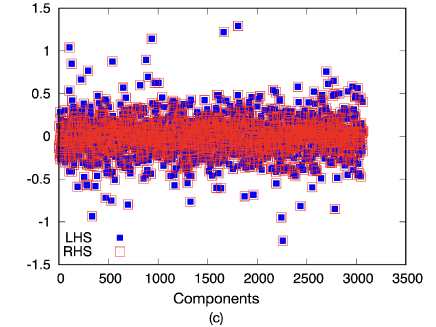
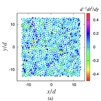
In this subsection, the validity of the theoretical rigidity presented in the previous section is demonstrated. For this purpose, at first, we examine the validity of Eq. (38), obtained by the eigenfunction expansion of the nonaffine displacements for RHS and by the simulation for LHS. Figures 3 (a) and (b) illustrate the nonaffine displacements on LHS and RHS of Eq. (38), respectively. In Figs. 3 (a) and (b), (x,y)๐‘ฅ๐‘ฆ(x,y) and โ„“โ„“\ell-components of dโ€‹๐’’ฬŠi/dโ€‹ฮณ๐‘‘subscriptฬŠ๐’’๐‘–๐‘‘๐›พd\mathring{\bm{q}}_{i}/d\gamma at ๐’“isubscript๐’“๐‘–\bm{r}_{i} are represented by vectors and colors, respectively. Figure 3 (c) shows the RHS and LHS of Eq. (38) against the components of the vectors whose orders follow Eq. (33), that is, the local order of the component follows x,y,๐‘ฅ๐‘ฆx,y, and โ„“โ„“\ell by fixing the particle number, and we align the components from the first particle to the N๐‘N-th particle without omitting modes with extremely small and zero eigenvalues. Figure 3 shows that the expression in Eq. (38) correctly reproduces the simulation results.
Refer to caption
Refer to caption
Refer to caption
Figure 3: Plots of nonaffine displacements on (a) RHS of Eq. (38) obtained by the eigenvalue analysis and (b) LHS of Eq. (38). The vector and color of each particle correspond to x,y,๐‘ฅ๐‘ฆx,y, and โ„“โ„“\ell-components of the eigenvector of the particle, respectively. Here, the magnitude of the vectors is magnified by 1.31.31.3 times for visualization. (c) Plots of the RHS (open symbols) and LHS (filled symbols) obtained by the simulation of Eq. (38) for each component whose order follows Eq. (33). These figures are based on numerical results for N=1024๐‘1024N=1024.

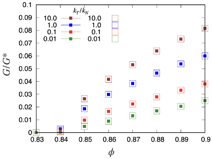
The dimensionless rigidity obtained from Eqs. (39),(40) and (44) with the aid of Gโˆ—:=kNโ€‹d1/2assignsuperscript๐บsubscript๐‘˜๐‘superscript๐‘‘12G^{*}:=k_{N}d^{1/2} is shown in Fig. 4. This indicates the quantitative agreement between the theoretical and numerical values.
Refer to caption
Figure 4: Plots of theoretical (Eq. (39): open symbols) and numerical (Eq. (16): filled symbols) G๐บG against ฯ•italic-ฯ•\phi for various kT/kNsubscript๐‘˜๐‘‡subscript๐‘˜๐‘k_{T}/k_{N}. The figure obtained by the numerical results for N=1024๐‘1024N=1024.

Therefore, the rigidity in the linear response regime can be determined completely using the Jacobian analysis. On the contrary to the previous studies Hern03 ; Olsson11 ; Otsuki11 , we should note that G๐บG is not proportional to ฯ•โˆ’ฯ•citalic-ฯ•subscriptitalic-ฯ•๐‘\phi-\phi_{c} for a large kT/kNsubscript๐‘˜๐‘‡subscript๐‘˜๐‘k_{T}/k_{N}, where ฯ•csubscriptitalic-ฯ•๐‘\phi_{c} is the critical fraction of jamming transition for frictional grains.
Refer to caption
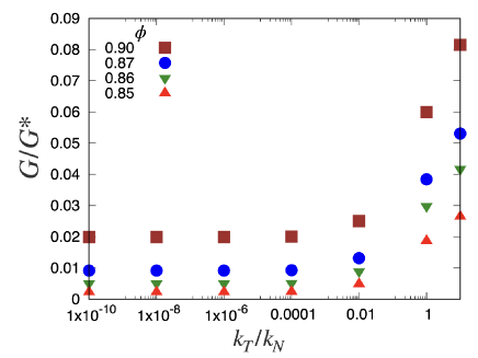
Figure 5: Plots of numerical G๐บG against kT/kNsubscript๐‘˜๐‘‡subscript๐‘˜๐‘k_{T}/k_{N} for various ฯ•italic-ฯ•\phi. The figure is obtained by the numerical results for N=4096๐‘4096N=4096.

As is expected, the rigidity G๐บG depends on kT/kNsubscript๐‘˜๐‘‡subscript๐‘˜๐‘k_{T}/k_{N} only little for kT/kNโ‰ค1.0ร—10โˆ’4subscript๐‘˜๐‘‡subscript๐‘˜๐‘1.0superscript104k_{T}/k_{N}\leq 1.0\times 10^{-4} (see Fig. 5), while G๐บG depends on kT/kNsubscript๐‘˜๐‘‡subscript๐‘˜๐‘k_{T}/k_{N} for kT/kN>10โˆ’4subscript๐‘˜๐‘‡subscript๐‘˜๐‘superscript104k_{T}/k_{N}>10^{-4}. We have confirmed that G๐บG smoothly approaches the frictionless value in the limit kTโ†’0โ†’subscript๐‘˜๐‘‡0k_{T}\to 0 in contrary to Refs. Otsuki17 ; Ishima20 . Here, G๐บG cannot be expressed as a factorization for large kT/kNsubscript๐‘˜๐‘‡subscript๐‘˜๐‘k_{T}/k_{N} 222 We have confirmed that the factorization Gโ€‹(ฯ•,kT/kN)=G0โ€‹(ฯ•)โ€‹๐’ขโ€‹(kT/kN)๐บitalic-ฯ•subscript๐‘˜๐‘‡subscript๐‘˜๐‘subscript๐บ0italic-ฯ•๐’ขsubscript๐‘˜๐‘‡subscript๐‘˜๐‘G(\phi,k_{T}/k_{N})=G_{0}(\phi)\mathcal{G}(k_{T}/k_{N}) is not held, where G0โ€‹(ฯ•)subscript๐บ0italic-ฯ•G_{0}(\phi) is the rigidity of frictionless system. . When we consider the effect of the dynamical friction, that is, slips between particles, the rigidity is discontinuously changed in the frictionless limit Otsuki17 ; Ishima20 . However, the rigidity continuously changes with kT/kNsubscript๐‘˜๐‘‡subscript๐‘˜๐‘k_{T}/k_{N} in our system and is smoothly connected to that of frictionless systems (kT=0subscript๐‘˜๐‘‡0k_{T}=0). Because our system can be regarded as having infinitely large static and dynamical frictional constants, there is no slip between the grains. Therefore, it might be natural for G๐บG to continuously change the limit for kT/kNโ†’0โ†’subscript๐‘˜๐‘‡subscript๐‘˜๐‘0k_{T}/k_{N}\to 0 in our system. In future work, we will consider the effects of slips, which are important for real frictional grains.

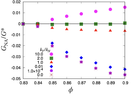
To clarify the contributions of nonaffine deformations to the rigidity, we plot GNAsubscript๐บNAG_{\textrm{NA}} defined in Eq. (41) against ฯ•italic-ฯ•\phi in Fig. 6, in which GNAsubscript๐บNAG_{\textrm{NA}} becomes large as ฯ•italic-ฯ•\phi increases. Remarkably, GNAsubscript๐บNAG_{\textrm{NA}} is positive for kT/kN>2.0subscript๐‘˜๐‘‡subscript๐‘˜๐‘2.0k_{T}/k_{N}>2.0, GNAโ‰ˆ0subscript๐บNA0G_{\textrm{NA}}\approx 0 at kT/kN=2.0subscript๐‘˜๐‘‡subscript๐‘˜๐‘2.0k_{T}/k_{N}=2.0, and GNAsubscript๐บNAG_{\textrm{NA}} is negative for kT/kN<2.0subscript๐‘˜๐‘‡subscript๐‘˜๐‘2.0k_{T}/k_{N}<2.0. The positive GNAsubscript๐บNAG_{\textrm{NA}} for a large kT/kNsubscript๐‘˜๐‘‡subscript๐‘˜๐‘k_{T}/k_{N} is counterintuitive, in which G๐บG increases from GAsubscript๐บAG_{\textrm{A}} even when the system is relaxed to the FB state. In the future, we must clarify the origin of this counterintuitive GNAsubscript๐บNAG_{\textrm{NA}}. We note that the negative GNAsubscript๐บNAG_{\textrm{NA}} for a small kT/kNsubscript๐‘˜๐‘‡subscript๐‘˜๐‘k_{T}/k_{N} can be understood by the relaxation process to look for a FB configuration after applying affine deformations to the system.
Refer to caption
Figure 6: Plots of GNAsubscript๐บNAG_{\textrm{NA}} against ฯ•italic-ฯ•\phi for various kT/kNsubscript๐‘˜๐‘‡subscript๐‘˜๐‘k_{T}/k_{N}. The figure is obtained by the numerical results for N=1024๐‘1024N=1024.

IV.2 Analysis of eigenvalues and eigenvectors

In Fig. 7 we present some typical right eigenvectors |RnโŸฉketsubscript๐‘…๐‘›\ket{R_{n}}, which was introduced in Eq. (21), and can be expressed as:

|RnโŸฉ=[๐‘นn,1๐‘นn,2โ‹ฎ๐‘นn,N],ketsubscript๐‘…๐‘›delimited-[]matrixsubscript๐‘น๐‘›1subscript๐‘น๐‘›2โ‹ฎsubscript๐‘น๐‘›๐‘\displaystyle\ket{R_{n}}=\left[\begin{matrix}\bm{R}_{n,1}\\ \bm{R}_{n,2}\\ \vdots\\ \bm{R}_{n,N}\end{matrix}\right], (48)

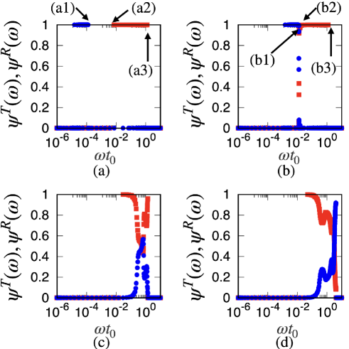
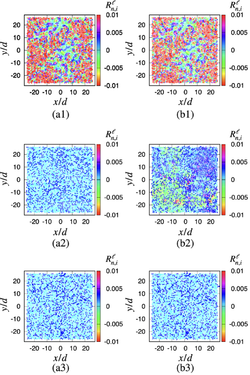
where ๐‘นn,i:=(Rn,ix,Rn,iy,Rn,iโ„“)Tassignsubscript๐‘น๐‘›๐‘–superscriptsuperscriptsubscript๐‘…๐‘›๐‘–๐‘ฅsuperscriptsubscript๐‘…๐‘›๐‘–๐‘ฆsuperscriptsubscript๐‘…๐‘›๐‘–โ„“T\bm{R}_{n,i}:=(R_{n,i}^{x},R_{n,i}^{y},R_{n,i}^{\ell})^{\textrm{T}}. Figure 7 illustrates vectors (Rn,ix,Rn,iy)Tsuperscriptsuperscriptsubscript๐‘…๐‘›๐‘–๐‘ฅsuperscriptsubscript๐‘…๐‘›๐‘–๐‘ฆT(R_{n,i}^{x},R_{n,i}^{y})^{\textrm{T}} and colors to characterize the rotation Rn,iโ„“superscriptsubscript๐‘…๐‘›๐‘–โ„“R_{n,i}^{\ell} of particle i๐‘–i for some characteristic ฯ‰nsubscript๐œ”๐‘›\omega_{n} with kT/kN=1.0ร—10โˆ’8subscript๐‘˜๐‘‡subscript๐‘˜๐‘1.0superscript108k_{T}/k_{N}=1.0\times 10^{-8} (Figs. 7 (a1)-(a3)) and kT/kN=1.0ร—10โˆ’4subscript๐‘˜๐‘‡subscript๐‘˜๐‘1.0superscript104k_{T}/k_{N}=1.0\times 10^{-4} (Figs. 7 (b1)-(b3)). Figures 7 (a1) and (b1) show the eigenvectors at ฯ‰nโ€‹t0=1.0ร—10โˆ’2subscript๐œ”๐‘›subscript๐‘ก01.0superscript102\omega_{n}t_{0}=1.0\times 10^{-2} and ฯ‰nโ€‹t0=1.0ร—10โˆ’4subscript๐œ”๐‘›subscript๐‘ก01.0superscript104\omega_{n}t_{0}=1.0\times 10^{-4}, respectively, which are dominated by the rotational modes. In Fig. 7 (a2), we confirm that the eigenvector at ฯ‰nโ€‹t0=1.3ร—10โˆ’2subscript๐œ”๐‘›subscript๐‘ก01.3superscript102\omega_{n}t_{0}=1.3\times 10^{-2} is expressed only by translational modes, whereas the eigenvector at ฯ‰nโ€‹t0=1.3ร—10โˆ’2subscript๐œ”๐‘›subscript๐‘ก01.3superscript102\omega_{n}t_{0}=1.3\times 10^{-2} shown in Fig. 7 (b2) is expressed as a coupling mode of the rotational and translational modes. In Figs. 7 (a3) and (b3), we show the eigenvectors at ฯ‰nโ€‹t0=1.0subscript๐œ”๐‘›subscript๐‘ก01.0\omega_{n}t_{0}=1.0 which are dominated by the translational modes.
Refer to caption
Figure 7: Plots of eigenvectors for ฯ•=0.90italic-ฯ•0.90\phi=0.90 with (a1) ฯ‰nโ€‹t0=1.0ร—10โˆ’4subscript๐œ”๐‘›subscript๐‘ก01.0superscript104\omega_{n}t_{0}=1.0\times 10^{-4}, (a2) 1.3ร—10โˆ’21.3superscript1021.3\times 10^{-2}, (a3) 1.01.01.0, (b1) 1.0ร—10โˆ’21.0superscript1021.0\times 10^{-2}, (b2) 1.3ร—10โˆ’21.3superscript1021.3\times 10^{-2}, and (b3) 1.01.01.0, where (a1)-(a3), and (b1)-(b3) are the results for kT/kN=1.0ร—10โˆ’8subscript๐‘˜๐‘‡subscript๐‘˜๐‘1.0superscript108k_{T}/k_{N}=1.0\times 10^{-8} and 1.0ร—10โˆ’41.0superscript1041.0\times 10^{-4}, respectively. Here, (Rn,ix,Rn,iy)Tsuperscriptsuperscriptsubscript๐‘…๐‘›๐‘–๐‘ฅsuperscriptsubscript๐‘…๐‘›๐‘–๐‘ฆT(R_{n,i}^{x},R_{n,i}^{y})^{\textrm{T}} and Rn,iโ„“superscriptsubscript๐‘…๐‘›๐‘–โ„“R_{n,i}^{\ell} are represented by vectors and colors for the i๐‘–i-th particle, respectively. Note that the magnitudes of the vectors are magnified by 505050 times for visualization. These figures are based on numerical results for N=4096๐‘4096N=4096.

To clarify the translational and rotational contributions at each eigenvalue, we compute the translational and rotational participation fractions Yunker11 ; Shiraishi19 defined as

ฯˆnTsuperscriptsubscript๐œ“๐‘›๐‘‡\displaystyle\psi_{n}^{T} :=โˆ‘i=1N[|Rn,ix|2+|Rn,iy|2],assignabsentsuperscriptsubscript๐‘–1๐‘delimited-[]superscriptsuperscriptsubscript๐‘…๐‘›๐‘–๐‘ฅ2superscriptsuperscriptsubscript๐‘…๐‘›๐‘–๐‘ฆ2\displaystyle:=\sum_{i=1}^{N}\left[|R_{n,i}^{x}|^{2}+|R_{n,i}^{y}|^{2}\right], (49)
ฯˆnRsuperscriptsubscript๐œ“๐‘›๐‘…\displaystyle\psi_{n}^{R} :=โˆ‘i=1N|Rn,iโ„“|2=1โˆ’ฯˆnT,assignabsentsuperscriptsubscript๐‘–1๐‘superscriptsuperscriptsubscript๐‘…๐‘›๐‘–โ„“21superscriptsubscript๐œ“๐‘›๐‘‡\displaystyle:=\sum_{i=1}^{N}|R_{n,i}^{\ell}|^{2}=1-\psi_{n}^{T}, (50)

respectively, where we have investigated the localization of the system with the participation ratio in Appendix E. Note that translational mode is dominant when ฯˆnTsuperscriptsubscript๐œ“๐‘›๐‘‡\psi_{n}^{T} is close to 111 and rotational mode is dominant when ฯˆnRsuperscriptsubscript๐œ“๐‘›๐‘…\psi_{n}^{R} is close to 111. ฯˆTโ€‹(ฯ‰)superscript๐œ“๐‘‡๐œ”\psi^{T}(\omega) and ฯˆRโ€‹(ฯ‰)superscript๐œ“๐‘…๐œ”\psi^{R}(\omega) are plotted for various kT/kNsubscript๐‘˜๐‘‡subscript๐‘˜๐‘k_{T}/k_{N} in Fig. 8, where

ฯˆTโ€‹(ฯ‰)::superscript๐œ“๐‘‡๐œ”absent\displaystyle\psi^{T}(\omega): =โˆ‘nโ€ฒโŸจฯˆnTโ€‹ฮดโ€‹(ฯ‰โˆ’ฯ‰n)โŸฉโˆ‘nโ€ฒโŸจฮดโ€‹(ฯ‰โˆ’ฯ‰n)โŸฉ,absentsuperscriptsubscript๐‘›โ€ฒdelimited-โŸจโŸฉsuperscriptsubscript๐œ“๐‘›๐‘‡๐›ฟ๐œ”subscript๐œ”๐‘›superscriptsubscript๐‘›โ€ฒdelimited-โŸจโŸฉ๐›ฟ๐œ”subscript๐œ”๐‘›\displaystyle=\frac{\sum_{n}\nolimits^{\prime}\langle\psi_{n}^{T}\delta(\omega-\omega_{n})\rangle}{\sum_{n}\nolimits^{\prime}\langle\delta(\omega-\omega_{n})\rangle}, (51)
ฯˆRโ€‹(ฯ‰)::superscript๐œ“๐‘…๐œ”absent\displaystyle\psi^{R}(\omega): =โˆ‘nโ€ฒโŸจฯˆnRโ€‹ฮดโ€‹(ฯ‰โˆ’ฯ‰n)โŸฉโˆ‘nโ€ฒโŸจฮดโ€‹(ฯ‰โˆ’ฯ‰n)โŸฉ.absentsuperscriptsubscript๐‘›โ€ฒdelimited-โŸจโŸฉsuperscriptsubscript๐œ“๐‘›๐‘…๐›ฟ๐œ”subscript๐œ”๐‘›superscriptsubscript๐‘›โ€ฒdelimited-โŸจโŸฉ๐›ฟ๐œ”subscript๐œ”๐‘›\displaystyle=\frac{\sum_{n}\nolimits^{\prime}\langle\psi_{n}^{R}\delta(\omega-\omega_{n})\rangle}{\sum_{n}\nolimits^{\prime}\langle\delta(\omega-\omega_{n})\rangle}. (52)

Here, ฯˆTsuperscript๐œ“๐‘‡\psi^{T} and ฯˆRsuperscript๐œ“๐‘…\psi^{R} are set to zero if there is no right eigenvalue for ฯ‰(s)<ฯ‰โ€‹t0<ฯ‰(s+1)superscript๐œ”๐‘ ๐œ”subscript๐‘ก0superscript๐œ”๐‘ 1\omega^{(s)}<\omega t_{0}<\omega^{(s+1)} with the s๐‘ s-th data point ฯ‰(s)superscript๐œ”๐‘ \omega^{(s)}. Here, we have used the following steps to determine each data point. First, we divided the data interval into 505050 parts on a logarithmic scale. Then we linearly re-divided the data interval from the highest frequency to the 10th highest frequency region. Finally, we also linearly re-divided the data interval of the log scale corresponding to 0.1โ€‹kT/kN<ฯ‰โ€‹t0<2โ€‹kT/kN0.1subscript๐‘˜๐‘‡subscript๐‘˜๐‘๐œ”subscript๐‘ก02subscript๐‘˜๐‘‡subscript๐‘˜๐‘0.1\sqrt{k_{T}/k_{N}}<\omega t_{0}<2\sqrt{k_{T}/k_{N}}. Note that for the linear re-division of the data, the regions were divided into 500500500 or 100100100 equally spaced inter-regional intervals for high frequency or 0.1โ€‹kT/kN<ฯ‰โ€‹t0<2โ€‹kT/kN0.1subscript๐‘˜๐‘‡subscript๐‘˜๐‘๐œ”subscript๐‘ก02subscript๐‘˜๐‘‡subscript๐‘˜๐‘0.1\sqrt{k_{T}/k_{N}}<\omega t_{0}<2\sqrt{k_{T}/k_{N}}, respectively.

Refer to caption
Figure 8: Semi-logarithmic plots of ฯˆTsuperscript๐œ“๐‘‡\psi^{T} (red filled squares) and ฯˆRsuperscript๐œ“๐‘…\psi^{R} (blue filled circles) against ฯ‰โ€‹t0๐œ”subscript๐‘ก0\omega t_{0} for ฯ•=0.90italic-ฯ•0.90\phi=0.90 at (a) kT/kN=1.0ร—10โˆ’8subscript๐‘˜๐‘‡subscript๐‘˜๐‘1.0superscript108k_{T}/k_{N}=1.0\times 10^{-8}, (b) 1.0ร—10โˆ’41.0superscript1041.0\times 10^{-4}, (c) 1.01.01.0, and (d) 10.010.010.0. The eigenvalues of (a1), (a2), (a3), (b1), (b2), and (b3) in these figures correspond to Figs. 7 (a1), (a2), (a3), (b1), (b2), and (b3), respectively. These figures are based on numerical results for N=4096๐‘4096N=4096.

As shown in Figs. 8 (a) and (b), we find the region of ฯˆRโ‰ƒ1similar-to-or-equalssuperscript๐œ“๐‘…1\psi^{R}\simeq 1 for low ฯ‰๐œ”\omega and kT/kN<1.0ร—10โˆ’4subscript๐‘˜๐‘‡subscript๐‘˜๐‘1.0superscript104k_{T}/k_{N}<1.0\times 10^{-4}. This region is referred to as Region I. We also find a region that satisfies ฯˆTโ‰ƒ1similar-to-or-equalssuperscript๐œ“๐‘‡1\psi^{T}\simeq 1 for high ฯ‰๐œ”\omega and kT/kN<1.0subscript๐‘˜๐‘‡subscript๐‘˜๐‘1.0k_{T}/k_{N}<1.0, in which the translational modes are dominant. This region is referred to as Region II. Here, three characteristic behaviors depend on kT/kNsubscript๐‘˜๐‘‡subscript๐‘˜๐‘k_{T}/k_{N} at ฯ•=0.90italic-ฯ•0.90\phi=0.90. First, the translational modes are separable from the rotational modes for kT/kNโ‰ค1.0ร—10โˆ’8subscript๐‘˜๐‘‡subscript๐‘˜๐‘1.0superscript108k_{T}/k_{N}\leq 1.0\times 10^{-8} because we need a small amount of energy to excite the rotational mode in nearly frictionless situations, as shown in Figs. 8 (a) and (b). Second, the translational and rotational contributions are not separated for 1.0ร—10โˆ’6โ‰คkT/kNโ‰ค1.0ร—10โˆ’21.0superscript106subscript๐‘˜๐‘‡subscript๐‘˜๐‘1.0superscript1021.0\times 10^{-6}\leq k_{T}/k_{N}\leq 1.0\times 10^{-2}. Third, the translational and rotational contributions are indistinguishable for kT/kNโ‰ฅ1.0subscript๐‘˜๐‘‡subscript๐‘˜๐‘1.0k_{T}/k_{N}\geq 1.0.

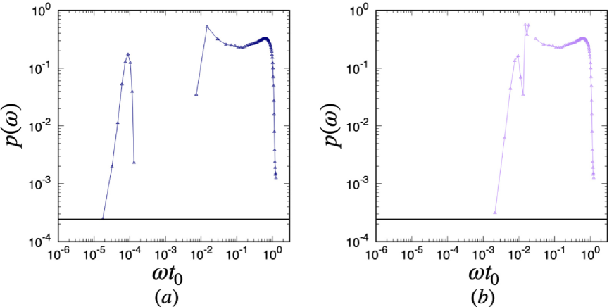
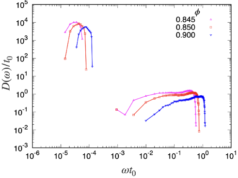
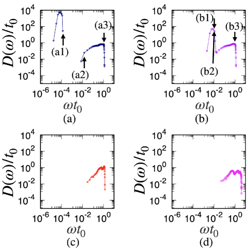
The DOS obtained from the Jacobian eigenvalues is shown in Fig. 9. Based on the results of ฯˆTโ€‹(ฯ‰)superscript๐œ“๐‘‡๐œ”\psi^{T}(\omega) and ฯˆRโ€‹(ฯ‰)superscript๐œ“๐‘…๐œ”\psi^{R}(\omega), the DOS is also separated into two regions for kT/kNโ‰ค1.0ร—10โˆ’8subscript๐‘˜๐‘‡subscript๐‘˜๐‘1.0superscript108k_{T}/k_{N}\leq 1.0\times 10^{-8}. The rotational band for low ฯ‰๐œ”\omega shifts to the high ฯ‰๐œ”\omega region as kT/kNsubscript๐‘˜๐‘‡subscript๐‘˜๐‘k_{T}/k_{N} increases (see Figs. 9 (a) and (b)). In Region II with a high ฯ‰๐œ”\omega (see Figs. 9 (a) and (b)), the DOS is almost independent of kT/kNsubscript๐‘˜๐‘‡subscript๐‘˜๐‘k_{T}/k_{N} in which the translational modes are dominant for kT/kNโ‰ค1.0ร—10โˆ’2subscript๐‘˜๐‘‡subscript๐‘˜๐‘1.0superscript102k_{T}/k_{N}\leq 1.0\times 10^{-2}. The distinctions between the two regions for the DOS are visible with a distinct gap between the adjacent regions for 1.0ร—10โˆ’10โ‰คkT/kNโ‰ค1.0ร—10โˆ’81.0superscript1010subscript๐‘˜๐‘‡subscript๐‘˜๐‘1.0superscript1081.0\times 10^{-10}\leq k_{T}/k_{N}\leq 1.0\times 10^{-8}. For 1.0ร—10โˆ’6โ‰คkT/kNโ‰ค1.0ร—10โˆ’21.0superscript106subscript๐‘˜๐‘‡subscript๐‘˜๐‘1.0superscript1021.0\times 10^{-6}\leq k_{T}/k_{N}\leq 1.0\times 10^{-2}; however, the high ฯ‰๐œ”\omega region of the DOS in Region I partially overlaps with the low ฯ‰๐œ”\omega region of Region II. Furthermore, Regions I and II are completely merged for kT/kNโ‰ฅ1.0subscript๐‘˜๐‘‡subscript๐‘˜๐‘1.0k_{T}/k_{N}\geq 1.0 (see Figs. 9 (c) and (d)). Isolated DOS bands for low ฯ‰๐œ”\omega have been observed in systems containing anisotropic grains, such as elliptical grains and dimers Yunker11 ; Schreck12 ; Shiraishi19 . However, to the best of our knowledge, there is no paper pointing out the existence of isolated bands of DOS in systems of frictional grains.
Refer to caption
Figure 9: Double logarithmic plots of Dโ€‹(ฯ‰)๐ท๐œ”D(\omega) against ฯ‰โ€‹t0๐œ”subscript๐‘ก0\omega t_{0} for ฯ•=0.90italic-ฯ•0.90\phi=0.90 at (a) kT/kN=1.0ร—10โˆ’8subscript๐‘˜๐‘‡subscript๐‘˜๐‘1.0superscript108k_{T}/k_{N}=1.0\times 10^{-8}, (b) 1.0ร—10โˆ’41.0superscript1041.0\times 10^{-4}, (c) 1.01.01.0, and (d) 10.010.010.0. The eigenvalues of (a1), (a2), (a3), (b1), (b2) and (b3) in these figures correspond to Figs. 7 (a1), (a2), (a3), (b1), (b2) and (b3), respectively. These figures are based on numerical results for N=4096๐‘4096N=4096.

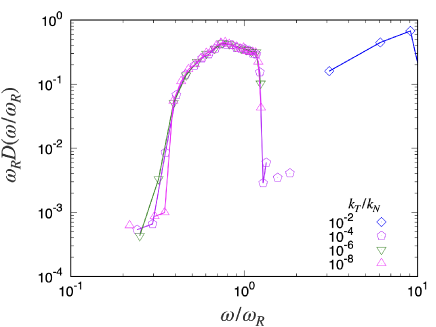
Because we have confirmed the existence of a peak of Dโ€‹(ฯ‰)๐ท๐œ”D(\omega) around ฯ‰โ€‹t0โ‰ƒ(kT/kN)1/2similar-to-or-equals๐œ”subscript๐‘ก0superscriptsubscript๐‘˜๐‘‡subscript๐‘˜๐‘12\omega t_{0}\simeq(k_{T}/k_{N})^{1/2}, Fig. 10 shows the scaling of the DOS in Region I by plotting ฯ‰Rโ€‹Dโ€‹(ฯ‰/ฯ‰R)subscript๐œ”๐‘…๐ท๐œ”subscript๐œ”๐‘…\omega_{R}D(\omega/\omega_{R}), where ฯ‰R:=kT/kNโ€‹t0โˆ’1assignsubscript๐œ”๐‘…subscript๐‘˜๐‘‡subscript๐‘˜๐‘superscriptsubscript๐‘ก01\omega_{R}:=\sqrt{k_{T}/k_{N}}t_{0}^{-1} 333 The reason why Dโ€‹(ฯ‰)๐ท๐œ”D(\omega) is multiplied by ฯ‰Rsubscript๐œ”๐‘…\omega_{R} in Fig. 10 is as follows. The integral value of the DOS within Region I โˆซI๐‘‘ฯ‰โ€‹Dโ€‹(ฯ‰)subscriptIdifferential-d๐œ”๐ท๐œ”\int_{\textrm{I}}d\omega D(\omega) is almost independent of kT/kNsubscript๐‘˜๐‘‡subscript๐‘˜๐‘k_{T}/k_{N}. Then, LHS can be rewritten as a variable โˆซI๐‘‘ฯ‰โ€‹Dโ€‹(ฯ‰)=โˆซI๐‘‘ฯ‰^โ€‹Dโˆ—โ€‹(ฯ‰^)subscriptIdifferential-d๐œ”๐ท๐œ”subscriptIdifferential-d^๐œ”superscript๐ท^๐œ”\int_{\textrm{I}}d\omega D(\omega)=\int_{\textrm{I}}d\hat{\omega}D^{*}(\hat{\omega}), where ฯ‰^:=ฯ‰/ฯ‰Rassign^๐œ”๐œ”subscript๐œ”๐‘…\hat{\omega}:=\omega/\omega_{R}, Dโˆ—โ€‹(ฯ‰^):=ฯ‰Rโ€‹Dโ€‹(ฯ‰/ฯ‰R)assignsuperscript๐ท^๐œ”subscript๐œ”๐‘…๐ท๐œ”subscript๐œ”๐‘…D^{*}(\hat{\omega}):=\omega_{R}D(\omega/\omega_{R}) and โˆซIsubscriptI\int_{\textrm{I}} represents the integral in Region I. . From Fig. 10 we have confirmed that ฯ‰Rโ€‹Dโ€‹(ฯ‰)subscript๐œ”๐‘…๐ท๐œ”\omega_{R}D(\omega) can be expressed as a universal scaling function of ฯ‰/ฯ‰R๐œ”subscript๐œ”๐‘…\omega/\omega_{R} for 0.1<ฯ‰/ฯ‰R<10.1๐œ”subscript๐œ”๐‘…10.1<\omega/\omega_{R}<1 and kT/kNโ‰ค0.01subscript๐‘˜๐‘‡subscript๐‘˜๐‘0.01k_{T}/k_{N}\leq 0.01.

Refer to caption
Figure 10: Scaling plots of ฯ‰Rโ€‹Dโ€‹(ฯ‰)subscript๐œ”๐‘…๐ท๐œ”\omega_{R}D(\omega) versus ฯ‰/ฯ‰R๐œ”subscript๐œ”๐‘…\omega/\omega_{R} for ฯ•=0.90italic-ฯ•0.90\phi=0.90 and various kT/kNsubscript๐‘˜๐‘‡subscript๐‘˜๐‘k_{T}/k_{N} in 0.1<ฯ‰/ฯ‰R<10.00.1๐œ”subscript๐œ”๐‘…10.00.1<\omega/\omega_{R}<10.0. The figure is based on numerical results for N=4096๐‘4096N=4096.

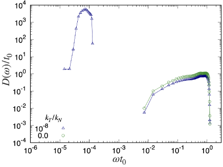
To clarify the behavior of the DOS in the frictionless limit, we compare the DOS for kT/kN=10โˆ’8subscript๐‘˜๐‘‡subscript๐‘˜๐‘superscript108k_{T}/k_{N}=10^{-8} with that for frictionless particles by plotting both cases, where we adopt the Hessian matrix to calculate the DOS for frictionless systems (see Fig. 11 and Appendix H). As expected, there is no singularity of the DOS for the translational mode, while the isolated rotational band in low ฯ‰๐œ”\omega is absent in frictionless particles, as shown in Fig. 11.
Refer to caption
Figure 11: Double logarithmic plots of Dโ€‹(ฯ‰)/t0๐ท๐œ”subscript๐‘ก0D(\omega)/t_{0} versus ฯ‰โ€‹t0๐œ”subscript๐‘ก0\omega t_{0} with ฯ•=0.90italic-ฯ•0.90\phi=0.90, where red circles are the DOS for frictional grains, while blue triangles are the DOS for frictionless grains. The figure is based on numerical results for N=4096๐‘4096N=4096.

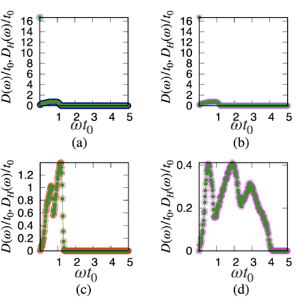
At the end of this subsection, we examine the usefulness of the effective Hessian โ„‹โ„‹\mathcal{H} introduced in Refs. Somfai07 ; Henkes10 ; Liu21 by comparing Dโ€‹(ฯ‰)๐ท๐œ”D(\omega) with DHโ€‹(ฯ‰)subscript๐ท๐ป๐œ”D_{H}(\omega), where DHโ€‹(ฯ‰)subscript๐ท๐ป๐œ”D_{H}(\omega) is the DOS obtained from โ„‹โ„‹\mathcal{H} (see Appendix H). As shown in Figs. 12 (a) and (b), Dโ€‹(ฯ‰)๐ท๐œ”D(\omega) and DHโ€‹(ฯ‰)subscript๐ท๐ป๐œ”D_{H}(\omega) for various kT/kNsubscript๐‘˜๐‘‡subscript๐‘˜๐‘k_{T}/k_{N} are almost identical. Here, the peak of the DOS near ฯ‰=0๐œ”0\omega=0 is caused by the rotational motion of the grains. This agreement between the Jacobian and Hessian analyses is natural because the configuration before the application of shear was prepared with frictionless particles, and the tangential displacement ฮพT,iโ€‹jsubscript๐œ‰๐‘‡๐‘–๐‘—\xi_{T,ij} is sufficiently small.

Refer to caption
Figure 12: Plots of Dโ€‹(ฯ‰)๐ท๐œ”D(\omega) (filled symbols) and DHโ€‹(ฯ‰)subscript๐ท๐ป๐œ”D_{H}(\omega) (open symbols) for ฯ•=0.90italic-ฯ•0.90\phi=0.90 at (a) kT/kN=1.0ร—10โˆ’8subscript๐‘˜๐‘‡subscript๐‘˜๐‘1.0superscript108k_{T}/k_{N}=1.0\times 10^{-8}, (b) 1.0ร—10โˆ’41.0superscript1041.0\times 10^{-4}, (c) 1.01.01.0, and (d) 10.0. These figures are based on numerical results for N=4096๐‘4096N=4096.

V Concluding Remarks

We analyzed the eigenmodes of the Jacobian and obtained an expression for the rigidity of amorphous solids of frictional particles under an infinitesimal strain. We reproduced the rigidity in the linear response regime using the eigenvalues and eigenfunctions of the Jacobian with modifications in the rotational part.

Further, we confirmed that the DOS can be divided into two regions for small kT/kNsubscript๐‘˜๐‘‡subscript๐‘˜๐‘k_{T}/k_{N}. In the low-frequency region (Region I), the rotation of the particles plays a dominant role. These modes are characterized by the frequency (kT/kN)1/2/t0superscriptsubscript๐‘˜๐‘‡subscript๐‘˜๐‘12subscript๐‘ก0(k_{T}/k_{N})^{1/2}/t_{0}. Region I merges into the high-frequency region (Region II) for large kT/kNsubscript๐‘˜๐‘‡subscript๐‘˜๐‘k_{T}/k_{N}, where Region II is dominated by translational modes.

It should be noted that our results are almost independent of system size, as shown in Appendix I. Moreover, we have briefly analyzed the density dependence of the DOS in Appendix J, where the rotational band shifts to a lower frequency region and the plateau of the translational band become longer as the density approaches the jamming point.

We have also confirmed that the results of our Jacobian analysis are almost equivalent to those of the Hessian matrix. This is because our preparation of the initial configuration of grains is made by frictionless grains. Nevertheless, we expect that the Hessian analysis might be sufficient for stable configurations of grains.

However, the applicability of this theory is limited. The method used in this study cannot be used for finite strains because it is obvious that the eigenvectors are not orthogonal in the sheared state. Moreover, there are plastic deformations of the grains under large strains, which were not considered in this study. Therefore, we cannot predict the correct value of the theoretical rigidity at the stress drop point. More importantly, the effect of the history dependence of the frictional force is significant even in the linear response regime, although we have ignored such contacts because of the difficulty in constructing a proper theory. This issue should be addressed in future studies Ishima22 .

VI ACKNOWLEDGMENTS

The authors thank N. Oyama and T. Kawasaki for fruitful discussions and useful comments. This work was partially supported by a Grant-in-Aid from the MEXT for Scientific Research (Grant No. JP22K03459, JP21H01006, and JP19K03670) and by the Grant-in-Aid from the Japan Society for Promotion of Science JSPS Research Fellow (Grant No. JP20J20292).

Appendix A Method of preparing configuration before applying the shear

In this Appendix, we summarize the method of preparing a stable configuration of grains before applying the shear. For this purpose, as the first step, we perform the relaxation for frictionless particles with the FIRE. As the second step, the system is relaxed taking into account the static friction between particles. In the first subsection, we summarize how to prepare the configurations of frictionless particles by the FIRE Bitzek06 . In the second subsection, we describe the details of the numerical method including the force with static friction.

A.1 Method of preparing configuration before applying shear by FIRE

At first, we place particles at random without any overlaps of particles with the initial fraction ฯ•ini=0.6subscriptitalic-ฯ•ini0.6\phi_{\textrm{ini}}=0.6. We increase the projected area fraction of the system by the increment of the fraction ฮฆ:=ฯ•Newโˆ’ฯ•Oldassignฮฆsuperscriptitalic-ฯ•Newsuperscriptitalic-ฯ•Old\Phi:=\phi^{\textrm{New}}-\phi^{\textrm{Old}} up to the target fraction ฯ•italic-ฯ•\phi, where ฯ•Oldsuperscriptitalic-ฯ•Old\phi^{\textrm{Old}} and ฯ•Newsuperscriptitalic-ฯ•New\phi^{\textrm{New}} are the projected area fraction of the system before and after each step of the increment, respectively. After each step of the increment, the system is relaxed by the FIRE Bitzek06 .

To implement the process of increasing the area fraction, we scale the system as

LNewsuperscript๐ฟNew\displaystyle L^{\textrm{New}} =LOldโ€‹ฯ•Oldฯ•New,absentsuperscript๐ฟOldsuperscriptitalic-ฯ•Oldsuperscriptitalic-ฯ•New\displaystyle=L^{\textrm{Old}}\sqrt{\frac{\phi^{\textrm{Old}}}{\phi^{\textrm{New}}}}, (1)
๐’“iNewsuperscriptsubscript๐’“๐‘–New\displaystyle\bm{r}_{i}^{\textrm{New}} =๐’“iOldโ€‹ฯ•Oldฯ•New,absentsuperscriptsubscript๐’“๐‘–Oldsuperscriptitalic-ฯ•Oldsuperscriptitalic-ฯ•New\displaystyle=\bm{r}_{i}^{\textrm{Old}}\sqrt{\frac{\phi^{\textrm{Old}}}{\phi^{\textrm{New}}}}, (2)

where LOld/LNewsuperscript๐ฟOldsuperscript๐ฟNewL^{\textrm{Old}}/L^{\textrm{New}} and ๐’“iOld/๐’“iNewsubscriptsuperscript๐’“Old๐‘–subscriptsuperscript๐’“New๐‘–\bm{r}^{\textrm{Old}}_{i}/\bm{r}^{\textrm{New}}_{i}are the linear system size and the position of the i๐‘–i-th particle before/after rescaling, respectively. We adopt ฮฆ=10โˆ’4ฮฆsuperscript104\Phi=10^{-4}. When there are overlaps between particles at ฯ•Newsuperscriptitalic-ฯ•New\phi^{\textrm{New}}, the system relaxes to a stable configuration with the aid of the FIRE.

The FIRE is a fast relaxation method of minimizing potentials Uโ€‹(๐’“)๐‘ˆ๐’“U(\bm{r}) depending on the configuration of the particles ๐’“:=(๐’“1T,๐’“2T,โ‹ฏ,๐’“NT)Tassign๐’“superscriptsuperscriptsubscript๐’“1Tsuperscriptsubscript๐’“2Tโ‹ฏsuperscriptsubscript๐’“๐‘TT\bm{r}:=(\bm{r}_{1}^{\textrm{T}},\bm{r}_{2}^{\textrm{T}},\cdots,\bm{r}_{N}^{\textrm{T}})^{\textrm{T}} with ๐’“i:=(rix,riy)T:=(xi,yi)Tassignsubscript๐’“๐‘–superscriptsuperscriptsubscript๐‘Ÿ๐‘–๐‘ฅsuperscriptsubscript๐‘Ÿ๐‘–๐‘ฆTassignsuperscriptsubscript๐‘ฅ๐‘–subscript๐‘ฆ๐‘–T\bm{r}_{i}:=(r_{i}^{x},r_{i}^{y})^{\textrm{T}}:=(x_{i},y_{i})^{\textrm{T}} Bitzek06 . Here, we use the Hertzian potential for Uโ€‹(๐’“)๐‘ˆ๐’“U(\bm{r}) which is defined as

Uโ€‹(๐’“):=25โ€‹kNโ€‹โˆ‘jโ‰ iฮพN,iโ€‹j5/2โ€‹ฮ˜โ€‹(diโ€‹j/2โˆ’|๐’“iโ€‹j|).assign๐‘ˆ๐’“25subscript๐‘˜๐‘subscript๐‘—๐‘–superscriptsubscript๐œ‰๐‘๐‘–๐‘—52ฮ˜subscript๐‘‘๐‘–๐‘—2subscript๐’“๐‘–๐‘—\displaystyle U(\bm{r}):=\frac{2}{5}k_{N}\sum_{j\neq i}\xi_{N,ij}^{5/2}\Theta(d_{ij}/2-|\bm{r}_{ij}|). (3)

Let us introduce ฮถ๐œ\zeta-component of the force FF,iฮถsuperscriptsubscript๐น๐น๐‘–๐œF_{F,i}^{\zeta} acting on the i๐‘–i-th particle as

FF,iฮถ::superscriptsubscript๐น๐น๐‘–๐œabsent\displaystyle F_{F,i}^{\zeta}: =โˆ’โˆ‚Uโˆ‚riฮถ=โˆ‘jโ‰ ikNโ€‹ฮพN,iโ€‹j3/2โ€‹niโ€‹jฮถโ€‹ฮ˜โ€‹(diโ€‹j/2โˆ’|๐’“iโ€‹j|),absent๐‘ˆsuperscriptsubscript๐‘Ÿ๐‘–๐œsubscript๐‘—๐‘–subscript๐‘˜๐‘superscriptsubscript๐œ‰๐‘๐‘–๐‘—32superscriptsubscript๐‘›๐‘–๐‘—๐œฮ˜subscript๐‘‘๐‘–๐‘—2subscript๐’“๐‘–๐‘—\displaystyle=-\frac{\partial U}{\partial r_{i}^{\zeta}}=\sum_{j\neq i}k_{N}\xi_{N,ij}^{3/2}n_{ij}^{\zeta}\Theta(d_{ij}/2-|\bm{r}_{ij}|), (4)

where ฮถ=x๐œ๐‘ฅ\zeta=x or y๐‘ฆy. Note that FF,iฮถsuperscriptsubscript๐น๐น๐‘–๐œF_{F,i}^{\zeta} only consists of the normal repulsive force. In the FIRE the position ๐’“๐’“\bm{r} and velocity ๐’—F:=(๐’—F,1,๐’—F,2,โ‹ฏ,๐’—F,N)Tassignsubscript๐’—๐นsuperscriptsubscript๐’—๐น1subscript๐’—๐น2โ‹ฏsubscript๐’—๐น๐‘T\bm{v}_{F}:=(\bm{v}_{F,1},\bm{v}_{F,2},\cdots,\bm{v}_{F,N})^{\textrm{T}} with ๐’—F,i:=(vF,ix,vF,iy)Tassignsubscript๐’—๐น๐‘–superscriptsuperscriptsubscript๐‘ฃ๐น๐‘–๐‘ฅsuperscriptsubscript๐‘ฃ๐น๐‘–๐‘ฆT\bm{v}_{F,i}:=(v_{F,i}^{x},v_{F,i}^{y})^{\textrm{T}} are updated by the following rules from (i) to (iv) with the variable time increment ฮ”โ€‹tFฮ”subscript๐‘ก๐น\Delta t_{F}. (i) The numerical integration via the velocity Verlet method is performed on ๐’“๐’“\bm{r} and ๐’—Fsubscript๐’—๐น\bm{v}_{F}:

riฮถsuperscriptsubscript๐‘Ÿ๐‘–๐œ\displaystyle r_{i}^{\zeta} โ†’riฮถ+ฮ”โ€‹tFโ€‹viฮถ+ฮ”โ€‹tF2โ€‹FF,iฮถโ€‹(๐’“)2โ€‹mi,โ†’absentsuperscriptsubscript๐‘Ÿ๐‘–๐œฮ”subscript๐‘ก๐นsuperscriptsubscript๐‘ฃ๐‘–๐œฮ”superscriptsubscript๐‘ก๐น2superscriptsubscript๐น๐น๐‘–๐œ๐’“2subscript๐‘š๐‘–\displaystyle\to r_{i}^{\zeta}+\Delta t_{F}v_{i}^{\zeta}+\Delta t_{F}^{2}\frac{F_{F,i}^{\zeta}(\bm{r})}{2m_{i}}, (5)
vF,iฮถsuperscriptsubscript๐‘ฃ๐น๐‘–๐œ\displaystyle v_{F,i}^{\zeta} โ†’vF,iฮถ+ฮ”โ€‹tFโ€‹FF,iฮถโ€‹(๐’“~)+FF,iฮถโ€‹(๐’“)2โ€‹mi,โ†’absentsuperscriptsubscript๐‘ฃ๐น๐‘–๐œฮ”subscript๐‘ก๐นsuperscriptsubscript๐น๐น๐‘–๐œ~๐’“superscriptsubscript๐น๐น๐‘–๐œ๐’“2subscript๐‘š๐‘–\displaystyle\to v_{F,i}^{\zeta}+\Delta t_{F}\frac{F_{F,i}^{\zeta}(\tilde{\bm{r}})+F_{F,i}^{\zeta}(\bm{r})}{2m_{i}}, (6)

where ๐’“~~๐’“\tilde{\bm{r}} is the updated configuration in Eq. (5). (ii) We calculate P:=๐‘ญFโ‹…๐’—Fassign๐‘ƒโ‹…subscript๐‘ญ๐นsubscript๐’—๐นP:=\bm{F}_{F}\cdot\bm{v}_{F}, where ๐‘ญF:=(๐‘ญF,1T,๐‘ญF,2T,โ‹ฏ,๐‘ญF,NT)Tassignsubscript๐‘ญ๐นsuperscriptsuperscriptsubscript๐‘ญ๐น1Tsuperscriptsubscript๐‘ญ๐น2Tโ‹ฏsuperscriptsubscript๐‘ญ๐น๐‘TT\bm{F}_{F}:=(\bm{F}_{F,1}^{\textrm{T}},\bm{F}_{F,2}^{\textrm{T}},\cdots,\bm{F}_{F,N}^{\textrm{T}})^{\textrm{T}} with ๐‘ญF,i:=(FF,ix,FF,iy)Tassignsubscript๐‘ญ๐น๐‘–superscriptsuperscriptsubscript๐น๐น๐‘–๐‘ฅsuperscriptsubscript๐น๐น๐‘–๐‘ฆT\bm{F}_{F,i}:=(F_{F,i}^{x},F_{F,i}^{y})^{\textrm{T}}. (iii) The velocity ๐’—Fsubscript๐’—๐น\bm{v}_{F} is updated as

๐’—F,iโ†’๐’—F,i+ฯ‡โ€‹(๐’—^F,iโˆ’๐‘ญ^F,i)โ€‹|๐’—F,i|,โ†’subscript๐’—๐น๐‘–subscript๐’—๐น๐‘–๐œ’subscript^๐’—๐น๐‘–subscript^๐‘ญ๐น๐‘–subscript๐’—๐น๐‘–\displaystyle\bm{v}_{F,i}\to\bm{v}_{F,i}+\chi(\hat{\bm{v}}_{F,i}-\hat{\bm{F}}_{F,i})|\bm{v}_{F,i}|, (7)

where ฯ‡๐œ’\chi is the relaxation parameter and ๐’‚^:=๐’‚/|๐’‚|assign^๐’‚๐’‚๐’‚\hat{\bm{a}}:=\bm{a}/|\bm{a}| for an arbitrary vector ๐’‚๐’‚\bm{a}. (iv) We update ฯ‡๐œ’\chi and ฮ”โ€‹tFฮ”subscript๐‘ก๐น\Delta t_{F} in the FIRE according to the positive or negative value of P๐‘ƒP. To speed up the relaxation when the motion is along a potential gradient, we increase ฮ”โ€‹tFฮ”subscript๐‘ก๐น\Delta t_{F}. Note that this process is performed only when the number of numerical integrations along the potential gradient is larger than a certain number of times Nminsubscript๐‘N_{\min} to stabilize the numerical calculation. To implement this update rule, if P>0๐‘ƒ0P>0 and the number of numerical integrations of P>0๐‘ƒ0P>0 is larger than Nminsubscript๐‘N_{\min}, ฮ”โ€‹tFฮ”subscript๐‘ก๐น\Delta t_{F} and ฯ‡๐œ’\chi are updated as

ฮ”โ€‹tFฮ”subscript๐‘ก๐น\displaystyle\Delta t_{F} โ†’minโก(ฮ”โ€‹tFโ€‹finc,ฮ”โ€‹tF,max),โ†’absentฮ”subscript๐‘ก๐นsubscript๐‘“incฮ”subscript๐‘ก๐น\displaystyle\to\min(\Delta t_{F}f_{\textrm{inc}},\Delta t_{F,\max}), (8)
ฯ‡๐œ’\displaystyle\chi โ†’ฯ‡โ€‹fฯ‡,โ†’absent๐œ’subscript๐‘“๐œ’\displaystyle\to\chi f_{\chi}, (9)

where minโก(a,b)๐‘Ž๐‘\min(a,b) is a selecting function of smaller one from a๐‘Ža and b๐‘b, the parameter fincsubscript๐‘“incf_{\textrm{inc}} is introduced to speed up the relaxation, and fฯ‡subscript๐‘“๐œ’f_{\chi}, and ฮ”โ€‹tF,maxฮ”subscript๐‘ก๐น\Delta t_{F,\max} are parameters to stabilize numerical calculations. Here, we adopt finc=1.1,fฯ‡=0.99,Nmin=5,ฮ”โ€‹tF,max=10โ€‹ฮ”โ€‹tF,iniformulae-sequencesubscript๐‘“inc1.1formulae-sequencesubscript๐‘“๐œ’0.99formulae-sequencesubscript๐‘5ฮ”subscript๐‘ก๐น10ฮ”subscript๐‘ก๐นinif_{\textrm{inc}}=1.1,f_{\chi}=0.99,N_{\min}=5,\Delta t_{F,\max}=10\Delta t_{F,\textrm{ini}}, and ฮ”โ€‹tF,ini=1.0ร—10โˆ’2โ€‹t0ฮ”subscript๐‘ก๐นini1.0superscript102subscript๐‘ก0\Delta t_{F,\textrm{ini}}=1.0\times 10^{-2}t_{0} Bitzek06 ; Saitoh19 . Note that Nminsubscript๐‘N_{\min} is necessary for the stability of the algorithm. In the case of Pโ‰ค0๐‘ƒ0P\leq 0, we set

๐’—Fsubscript๐’—๐น\displaystyle\bm{v}_{F} โ†’๐ŸŽ,โ†’absent0\displaystyle\to\bm{0}, (10)
ฯ‡๐œ’\displaystyle\chi โ†’ฯ‡start,โ†’absentsubscript๐œ’start\displaystyle\to\chi_{\textrm{start}}, (11)
ฮ”โ€‹tFฮ”subscript๐‘ก๐น\displaystyle\Delta t_{F} โ†’ฮ”โ€‹tFโ€‹fdec,โ†’absentฮ”subscript๐‘ก๐นsubscript๐‘“dec\displaystyle\to\Delta t_{F}f_{\textrm{dec}}, (12)

where we adopt fdec=0.5subscript๐‘“dec0.5f_{\textrm{dec}}=0.5 and ฯ‡start=0.1subscript๐œ’start0.1\chi_{\textrm{start}}=0.1 Bitzek06 ; Saitoh19 .

We repeat the operations (i) through (iv) until |FF,iฮถ|<FThsuperscriptsubscript๐น๐น๐‘–๐œsubscript๐นTh|F_{F,i}^{\zeta}|<F_{\textrm{Th}} for arbitrary i๐‘–i and ฮถ๐œ\zeta. Note that we have used the initial values for ฮ”โ€‹tF=ฮ”โ€‹tF,iniฮ”subscript๐‘ก๐นฮ”subscript๐‘ก๐นini\Delta t_{F}=\Delta t_{F,\textrm{ini}} and ฯ‡=ฯ‡start๐œ’subscript๐œ’start\chi=\chi_{\textrm{start}} at the starting point of the FIRE. Here, ๐’“๐’“\bm{r} is given and we set ๐’—F=๐ŸŽsubscript๐’—๐น0\bm{v}_{F}=\bm{0} at the starting point of the FIRE.

A.2 Numerical method for relaxation of configuration of frictional particles

After we obtain a stable configuration of frictionless particles at a target fraction in terms of the FIRE, we consider the effect of static friction in the relaxation process of frictional particles. The time evolution of the system is given by Eqs. (1)-(8) until F~iฮฑ<FThsuperscriptsubscript~๐น๐‘–๐›ผsubscript๐นTh\tilde{F}_{i}^{\alpha}<F_{\textrm{Th}} for arbitrary i๐‘–i and ฮฑ๐›ผ\alpha. For the time integration, we adopt the velocity Verlet method with the time increment ฮ”โ€‹t=1.0ร—10โˆ’2โ€‹t0ฮ”๐‘ก1.0superscript102subscript๐‘ก0\Delta t=1.0\times 10^{-2}t_{0}.

Appendix B Velocity Verlet method in our system

In this Appendix, we first verify the accuracy of the velocity Verlet method. Next, we summarize the implementation of the velocity Verlet method. To simplify the notation, we introduce the generalized force ๐’‡~:=(๐’‡~1T,๐’‡~2T,โ‹ฏ,๐’‡~NT)Tassign~๐’‡superscriptsuperscriptsubscript~๐’‡1Tsuperscriptsubscript~๐’‡2Tโ‹ฏsuperscriptsubscript~๐’‡๐‘TT\tilde{\bm{f}}:=(\tilde{\bm{f}}_{1}^{\textrm{T}},\tilde{\bm{f}}_{2}^{\textrm{T}},\cdots,\tilde{\bm{f}}_{N}^{\textrm{T}})^{\textrm{T}} with ๐’‡~i:=(f~ix,f~iy,f~iโ„“)T:=(F~ix/mix,F~iy/miy,F~iโ„“/miโ„“)Tassignsubscript~๐’‡๐‘–superscriptsuperscriptsubscript~๐‘“๐‘–๐‘ฅsuperscriptsubscript~๐‘“๐‘–๐‘ฆsuperscriptsubscript~๐‘“๐‘–โ„“๐‘‡assignsuperscriptsuperscriptsubscript~๐น๐‘–๐‘ฅsuperscriptsubscript๐‘š๐‘–๐‘ฅsuperscriptsubscript~๐น๐‘–๐‘ฆsuperscriptsubscript๐‘š๐‘–๐‘ฆsuperscriptsubscript~๐น๐‘–โ„“superscriptsubscript๐‘š๐‘–โ„“T\tilde{\bm{f}}_{i}:=(\tilde{f}_{i}^{x},\tilde{f}_{i}^{y},\tilde{f}_{i}^{\ell})^{T}:=(\tilde{F}_{i}^{x}/m_{i}^{x},\tilde{F}_{i}^{y}/m_{i}^{y},\tilde{F}_{i}^{\ell}/m_{i}^{\ell})^{\textrm{T}} in this Appendix, where miฮฑsuperscriptsubscript๐‘š๐‘–๐›ผm_{i}^{\alpha} is misubscript๐‘š๐‘–m_{i} for ฮฑ=x,y๐›ผ๐‘ฅ๐‘ฆ\alpha=x,y and 4โ€‹Ii/di24subscript๐ผ๐‘–superscriptsubscript๐‘‘๐‘–24I_{i}/d_{i}^{2} for ฮฑ=โ„“๐›ผโ„“\alpha=\ell. Note that F~iฮฑsuperscriptsubscript~๐น๐‘–๐›ผ\tilde{F}_{i}^{\alpha} is the generalized force which depends on ๐’’๐’’\bm{q} and ๐’’ห™ห™๐’’\dot{\bm{q}} as in Eqs. (3)-(8), where ๐’‚ห™:=dโ€‹๐’‚/dโ€‹tassignห™๐’‚๐‘‘๐’‚๐‘‘๐‘ก\dot{\bm{a}}:=d\bm{a}/dt for an arbitrary vector ๐’‚๐’‚\bm{a}.

B.1 Accuracy of the velocity Verlet method for the force depending on the velocity

In this subsection, we check the accuracy of the velocity Verlet method for the force depending on the velocity with the aid of discretization based on the Taylor expansion. The velocity Verlte method is given by a set of equations

qiฮฑโ€‹(t+ฮ”โ€‹t)superscriptsubscript๐‘ž๐‘–๐›ผ๐‘กฮ”๐‘ก\displaystyle q_{i}^{\alpha}(t+\Delta t) =qiฮฑโ€‹(t)+ฮ”โ€‹tโ€‹qห™iฮฑโ€‹(t)+12โ€‹ฮ”โ€‹t2โ€‹f~iฮฑโ€‹(t),absentsuperscriptsubscript๐‘ž๐‘–๐›ผ๐‘กฮ”๐‘กsuperscriptsubscriptห™๐‘ž๐‘–๐›ผ๐‘ก12ฮ”superscript๐‘ก2superscriptsubscript~๐‘“๐‘–๐›ผ๐‘ก\displaystyle=q_{i}^{\alpha}(t)+\Delta t\dot{q}_{i}^{\alpha}(t)+\frac{1}{2}\Delta t^{2}\tilde{f}_{i}^{\alpha}(t), (13)
qห™iฮฑโ€‹(t+ฮ”โ€‹t)superscriptsubscriptห™๐‘ž๐‘–๐›ผ๐‘กฮ”๐‘ก\displaystyle\dot{q}_{i}^{\alpha}(t+\Delta t) =qห™iฮฑโ€‹(t)+ฮ”โ€‹tโ€‹f~iฮฑโ€‹(t)+f~iฮฑโ€‹(t+ฮ”โ€‹t)2.absentsuperscriptsubscriptห™๐‘ž๐‘–๐›ผ๐‘กฮ”๐‘กsuperscriptsubscript~๐‘“๐‘–๐›ผ๐‘กsuperscriptsubscript~๐‘“๐‘–๐›ผ๐‘กฮ”๐‘ก2\displaystyle=\dot{q}_{i}^{\alpha}\left(t\right)+\Delta t\frac{\tilde{f}_{i}^{\alpha}(t)+\tilde{f}_{i}^{\alpha}(t+\Delta t)}{2}. (14)

The first equation is called the velocity Velret equation for qiฮฑโ€‹(t)superscriptsubscript๐‘ž๐‘–๐›ผ๐‘กq_{i}^{\alpha}(t) and the second one is the equation for qห™iฮฑโ€‹(t)superscriptsubscriptห™๐‘ž๐‘–๐›ผ๐‘ก\dot{q}_{i}^{\alpha}(t). It is known that the velocity Verlet algorithm has the accuracy of Oโ€‹(ฮ”โ€‹t2)๐‘‚ฮ”superscript๐‘ก2O(\Delta t^{2}) in Hamiltonian systems Swope82 , but the accuracy of this method for dissipative dynamics is little known. Therefore, we clarify the accuracy of this method in this Appendix.

Here, we show from the Taylor expansion that the velocity Verlet method has a second-order and first-order accuracies of ฮ”โ€‹tฮ”๐‘ก\Delta t for ๐’’๐’’\bm{q} and ๐’’ห™ห™๐’’\dot{\bm{q}}, respectively. Based on the Taylor expansion of qiฮฑโ€‹(t+ฮ”โ€‹t)superscriptsubscript๐‘ž๐‘–๐›ผ๐‘กฮ”๐‘กq_{i}^{\alpha}(t+\Delta t), we obtain

qiฮฑโ€‹(t+ฮ”โ€‹t)superscriptsubscript๐‘ž๐‘–๐›ผ๐‘กฮ”๐‘ก\displaystyle q_{i}^{\alpha}(t+\Delta t) =qiฮฑโ€‹(t)+ฮ”โ€‹tโ€‹qห™iฮฑโ€‹(t)+12โ€‹ฮ”โ€‹t2โ€‹qยจiฮฑโ€‹(t)+Oโ€‹(ฮ”โ€‹t3)absentsuperscriptsubscript๐‘ž๐‘–๐›ผ๐‘กฮ”๐‘กsuperscriptsubscriptห™๐‘ž๐‘–๐›ผ๐‘ก12ฮ”superscript๐‘ก2superscriptsubscriptยจ๐‘ž๐‘–๐›ผ๐‘ก๐‘‚ฮ”superscript๐‘ก3\displaystyle=q_{i}^{\alpha}(t)+\Delta t\dot{q}_{i}^{\alpha}(t)+\frac{1}{2}\Delta t^{2}\ddot{q}_{i}^{\alpha}(t)+O(\Delta t^{3})
=qiฮฑโ€‹(t)+ฮ”โ€‹tโ€‹qห™iฮฑโ€‹(t)+12โ€‹ฮ”โ€‹t2โ€‹f~iฮฑโ€‹(t)+Oโ€‹(ฮ”โ€‹t3),absentsuperscriptsubscript๐‘ž๐‘–๐›ผ๐‘กฮ”๐‘กsuperscriptsubscriptห™๐‘ž๐‘–๐›ผ๐‘ก12ฮ”superscript๐‘ก2superscriptsubscript~๐‘“๐‘–๐›ผ๐‘ก๐‘‚ฮ”superscript๐‘ก3\displaystyle=q_{i}^{\alpha}(t)+\Delta t\dot{q}_{i}^{\alpha}(t)+\frac{1}{2}\Delta t^{2}\tilde{f}_{i}^{\alpha}(t)+O(\Delta t^{3}), (15)

where Aห™:=dโ€‹A/dโ€‹tassignห™๐ด๐‘‘๐ด๐‘‘๐‘ก\dot{A}:=dA/dt for an arbitrary function A๐ดA. We can obtain the quadratic precision of ฮ”โ€‹tฮ”๐‘ก\Delta t for qiฮฑโ€‹(t+ฮ”โ€‹t)superscriptsubscript๐‘ž๐‘–๐›ผ๐‘กฮ”๐‘กq_{i}^{\alpha}(t+\Delta t), because the RHS of Eq. (15) is a function of current time t๐‘กt.

On the other hand, based on the Taylor expansion of qห™iฮฑโ€‹(t+ฮ”โ€‹t)superscriptsubscriptห™๐‘ž๐‘–๐›ผ๐‘กฮ”๐‘ก\dot{q}_{i}^{\alpha}(t+\Delta t), we obtain

qห™iฮฑโ€‹(t+ฮ”โ€‹t)superscriptsubscriptห™๐‘ž๐‘–๐›ผ๐‘กฮ”๐‘ก\displaystyle\dot{q}_{i}^{\alpha}(t+\Delta t) =qห™iฮฑโ€‹(t)+ฮ”โ€‹tโ€‹qยจiฮฑโ€‹(t)+12โ€‹ฮ”โ€‹t2โ€‹qห™ห™ห™iฮฑโ€‹(t)+Oโ€‹(ฮ”โ€‹t3)absentsuperscriptsubscriptห™๐‘ž๐‘–๐›ผ๐‘กฮ”๐‘กsuperscriptsubscriptยจ๐‘ž๐‘–๐›ผ๐‘ก12ฮ”superscript๐‘ก2superscriptsubscriptห™ห™ห™๐‘ž๐‘–๐›ผ๐‘ก๐‘‚ฮ”superscript๐‘ก3\displaystyle=\dot{q}_{i}^{\alpha}(t)+\Delta t\ddot{q}_{i}^{\alpha}(t)+\frac{1}{2}\Delta t^{2}\dddot{q}_{i}^{\alpha}(t)+O(\Delta t^{3})
=qห™iฮฑโ€‹(t)+ฮ”โ€‹tโ€‹f~iฮฑโ€‹(t)+12โ€‹ฮ”โ€‹t2โ€‹f~ห™iฮฑโ€‹(t)+Oโ€‹(ฮ”โ€‹t3).absentsuperscriptsubscriptห™๐‘ž๐‘–๐›ผ๐‘กฮ”๐‘กsuperscriptsubscript~๐‘“๐‘–๐›ผ๐‘ก12ฮ”superscript๐‘ก2superscriptsubscriptห™~๐‘“๐‘–๐›ผ๐‘ก๐‘‚ฮ”superscript๐‘ก3\displaystyle=\dot{q}_{i}^{\alpha}(t)+\Delta t\tilde{f}_{i}^{\alpha}(t)+\frac{1}{2}\Delta t^{2}\dot{\tilde{f}}_{i}^{\alpha}(t)+O(\Delta t^{3}). (16)

By using f~iฮฑโ€‹(t+ฮ”โ€‹t)=f~iฮฑโ€‹(t)+ฮ”โ€‹tโ€‹f~ห™iฮฑโ€‹(t)+Oโ€‹(ฮ”โ€‹t2)superscriptsubscript~๐‘“๐‘–๐›ผ๐‘กฮ”๐‘กsuperscriptsubscript~๐‘“๐‘–๐›ผ๐‘กฮ”๐‘กsuperscriptsubscriptห™~๐‘“๐‘–๐›ผ๐‘ก๐‘‚ฮ”superscript๐‘ก2\tilde{f}_{i}^{\alpha}(t+\Delta t)=\tilde{f}_{i}^{\alpha}(t)+\Delta t\dot{\tilde{f}}_{i}^{\alpha}(t)+O(\Delta t^{2}), we evaluate f~ห™iฮฑโ€‹(t)superscriptsubscriptห™~๐‘“๐‘–๐›ผ๐‘ก\dot{\tilde{f}}_{i}^{\alpha}(t) as

f~ห™iฮฑโ€‹(t)=f~iฮฑโ€‹(t+ฮ”โ€‹t)โˆ’f~iฮฑโ€‹(t)ฮ”โ€‹t+Oโ€‹(ฮ”โ€‹t).superscriptsubscriptห™~๐‘“๐‘–๐›ผ๐‘กsuperscriptsubscript~๐‘“๐‘–๐›ผ๐‘กฮ”๐‘กsuperscriptsubscript~๐‘“๐‘–๐›ผ๐‘กฮ”๐‘ก๐‘‚ฮ”๐‘ก\displaystyle\dot{\tilde{f}}_{i}^{\alpha}(t)=\frac{\tilde{f}_{i}^{\alpha}(t+\Delta t)-\tilde{f}_{i}^{\alpha}(t)}{\Delta t}+O(\Delta t). (17)

Substituting Eq. (17) into Eq. (16), we obtain Swope82

qห™iฮฑโ€‹(t+ฮ”โ€‹t)superscriptsubscriptห™๐‘ž๐‘–๐›ผ๐‘กฮ”๐‘ก\displaystyle\dot{q}_{i}^{\alpha}(t+\Delta t) =qห™iฮฑโ€‹(t)+ฮ”โ€‹tโ€‹f~iฮฑโ€‹(t+ฮ”โ€‹t)+f~iฮฑโ€‹(t)2+Oโ€‹(ฮ”โ€‹t3).absentsuperscriptsubscriptห™๐‘ž๐‘–๐›ผ๐‘กฮ”๐‘กsuperscriptsubscript~๐‘“๐‘–๐›ผ๐‘กฮ”๐‘กsuperscriptsubscript~๐‘“๐‘–๐›ผ๐‘ก2๐‘‚ฮ”superscript๐‘ก3\displaystyle=\dot{q}_{i}^{\alpha}(t)+\Delta t\frac{\tilde{f}_{i}^{\alpha}(t+\Delta t)+\tilde{f}_{i}^{\alpha}(t)}{2}+O(\Delta t^{3}). (18)

If the force f~iฮฑโ€‹(t+ฮ”โ€‹t)superscriptsubscript~๐‘“๐‘–๐›ผ๐‘กฮ”๐‘ก\tilde{f}_{i}^{\alpha}(t+\Delta t) is independent of ๐’’ห™ห™๐’’\dot{\bm{q}}, we can obtain f~iฮฑโ€‹(๐’’โ€‹(t+ฮ”โ€‹t))superscriptsubscript~๐‘“๐‘–๐›ผ๐’’๐‘กฮ”๐‘ก\tilde{f}_{i}^{\alpha}(\bm{q}(t+\Delta t)) from ๐’’โ€‹(t+ฮ”โ€‹t)๐’’๐‘กฮ”๐‘ก\bm{q}(t+\Delta t) with the aid of Eq. (15) Swope82 . However, if f~iฮฑโ€‹(t+ฮ”โ€‹t)superscriptsubscript~๐‘“๐‘–๐›ผ๐‘กฮ”๐‘ก\tilde{f}_{i}^{\alpha}(t+\Delta t) depends on ๐’’ห™ห™๐’’\dot{\bm{q}}, we have to evaluate f~iฮฑโ€‹(๐’’โ€‹(t+ฮ”โ€‹t),๐’’ห™โ€‹(t+ฮ”โ€‹t))superscriptsubscript~๐‘“๐‘–๐›ผ๐’’๐‘กฮ”๐‘กห™๐’’๐‘กฮ”๐‘ก\tilde{f}_{i}^{\alpha}(\bm{q}(t+\Delta t),\dot{\bm{q}}(t+\Delta t)), because f~iฮฑโ€‹(๐’’โ€‹(t+ฮ”โ€‹t),๐’’ห™โ€‹(t+ฮ”โ€‹t))superscriptsubscript~๐‘“๐‘–๐›ผ๐’’๐‘กฮ”๐‘กห™๐’’๐‘กฮ”๐‘ก\tilde{f}_{i}^{\alpha}(\bm{q}(t+\Delta t),\dot{\bm{q}}(t+\Delta t)) requires LHS of Eq. (18). Thus, we adopt the following replacements:

f~iฮฑโ€‹(t+ฮ”โ€‹t)::superscriptsubscript~๐‘“๐‘–๐›ผ๐‘กฮ”๐‘กabsent\displaystyle\tilde{f}_{i}^{\alpha}(t+\Delta t): =f~iฮฑโ€‹(๐’’โ€‹(t+ฮ”โ€‹t),๐’’ห™โ€‹(t+ฮ”โ€‹t))โ†’f~iฮฑโ€‹(๐’’โ€‹(t+ฮ”โ€‹t),๐‘ธห™โ€‹(t)),absentsuperscriptsubscript~๐‘“๐‘–๐›ผ๐’’๐‘กฮ”๐‘กห™๐’’๐‘กฮ”๐‘กโ†’superscriptsubscript~๐‘“๐‘–๐›ผ๐’’๐‘กฮ”๐‘กห™๐‘ธ๐‘ก\displaystyle=\tilde{f}_{i}^{\alpha}(\bm{q}(t+\Delta t),\dot{\bm{q}}(t+\Delta t))\to\tilde{f}_{i}^{\alpha}(\bm{q}(t+\Delta t),\dot{\bm{Q}}(t)), (19)
f~iฮฑโ€‹(t)::superscriptsubscript~๐‘“๐‘–๐›ผ๐‘กabsent\displaystyle\tilde{f}_{i}^{\alpha}(t): =f~iฮฑโ€‹(๐’’โ€‹(t),๐’’ห™โ€‹(t))โ†’f~iฮฑโ€‹(๐’’โ€‹(t),๐‘ธห™โ€‹(tโˆ’ฮ”โ€‹t)),absentsuperscriptsubscript~๐‘“๐‘–๐›ผ๐’’๐‘กห™๐’’๐‘กโ†’superscriptsubscript~๐‘“๐‘–๐›ผ๐’’๐‘กห™๐‘ธ๐‘กฮ”๐‘ก\displaystyle=\tilde{f}_{i}^{\alpha}(\bm{q}(t),\dot{\bm{q}}(t))\to\tilde{f}_{i}^{\alpha}(\bm{q}(t),\dot{\bm{Q}}(t-\Delta t)), (20)

where we have introduced

Qห™iฮฑโ€‹(t)::superscriptsubscriptห™๐‘„๐‘–๐›ผ๐‘กabsent\displaystyle\dot{Q}_{i}^{\alpha}(t): =qห™iฮฑโ€‹(t)+ฮ”โ€‹tโ€‹f~iฮฑโ€‹(๐’’โ€‹(t),๐‘ธห™โ€‹(tโˆ’ฮ”โ€‹t))2,absentsuperscriptsubscriptห™๐‘ž๐‘–๐›ผ๐‘กฮ”๐‘กsuperscriptsubscript~๐‘“๐‘–๐›ผ๐’’๐‘กห™๐‘ธ๐‘กฮ”๐‘ก2\displaystyle=\dot{q}_{i}^{\alpha}(t)+\Delta t\frac{\tilde{f}_{i}^{\alpha}(\bm{q}(t),\dot{\bm{Q}}(t-\Delta t))}{2}, (21)
Qห™iฮฑโ€‹(tโˆ’ฮ”โ€‹t)::superscriptsubscriptห™๐‘„๐‘–๐›ผ๐‘กฮ”๐‘กabsent\displaystyle\dot{Q}_{i}^{\alpha}(t-\Delta t): =qห™iฮฑโ€‹(tโˆ’ฮ”โ€‹t)+ฮ”โ€‹tโ€‹f~iฮฑโ€‹(๐’’โ€‹(tโˆ’ฮ”โ€‹t),๐‘ธห™โ€‹(tโˆ’2โ€‹ฮ”โ€‹t))2.absentsuperscriptsubscriptห™๐‘ž๐‘–๐›ผ๐‘กฮ”๐‘กฮ”๐‘กsuperscriptsubscript~๐‘“๐‘–๐›ผ๐’’๐‘กฮ”๐‘กห™๐‘ธ๐‘ก2ฮ”๐‘ก2\displaystyle=\dot{q}_{i}^{\alpha}(t-\Delta t)+\Delta t\frac{\tilde{f}_{i}^{\alpha}(\bm{q}(t-\Delta t),\dot{\bm{Q}}(t-2\Delta t))}{2}. (22)

Here, the difference between f~iฮฑโ€‹(๐’’โ€‹(t+ฮ”โ€‹t),๐’’ห™โ€‹(t+ฮ”โ€‹t))superscriptsubscript~๐‘“๐‘–๐›ผ๐’’๐‘กฮ”๐‘กห™๐’’๐‘กฮ”๐‘ก\tilde{f}_{i}^{\alpha}(\bm{q}(t+\Delta t),\dot{\bm{q}}(t+\Delta t)) and f~iฮฑโ€‹(๐’’โ€‹(t+ฮ”โ€‹t),๐‘ธห™โ€‹(t))superscriptsubscript~๐‘“๐‘–๐›ผ๐’’๐‘กฮ”๐‘กห™๐‘ธ๐‘ก\tilde{f}_{i}^{\alpha}(\bm{q}(t+\Delta t),\dot{\bm{Q}}(t)) caused by Eq. (19) is given by

ฮ”โ€‹f~iฮฑโ€‹(t+ฮ”โ€‹t)ฮ”superscriptsubscript~๐‘“๐‘–๐›ผ๐‘กฮ”๐‘ก\displaystyle\Delta\tilde{f}_{i}^{\alpha}(t+\Delta t) :=f~iฮฑโ€‹(๐’’โ€‹(t+ฮ”โ€‹t),๐’’ห™โ€‹(t+ฮ”โ€‹t))โˆ’f~iฮฑโ€‹(๐’’โ€‹(t+ฮ”โ€‹t),๐‘ธห™โ€‹(t))assignabsentsuperscriptsubscript~๐‘“๐‘–๐›ผ๐’’๐‘กฮ”๐‘กห™๐’’๐‘กฮ”๐‘กsuperscriptsubscript~๐‘“๐‘–๐›ผ๐’’๐‘กฮ”๐‘กห™๐‘ธ๐‘ก\displaystyle:=\tilde{f}_{i}^{\alpha}(\bm{q}(t+\Delta t),\dot{\bm{q}}(t+\Delta t))-\tilde{f}_{i}^{\alpha}(\bm{q}(t+\Delta t),\dot{\bm{Q}}(t))
=f~iฮฑโ€‹(๐’’โ€‹(t+ฮ”โ€‹t),๐’’ห™โ€‹(t)+ฮ”โ€‹tโ€‹๐’‡~โ€‹(t)+Oโ€‹(ฮ”โ€‹t2))โˆ’f~iฮฑโ€‹(๐’’โ€‹(t+ฮ”โ€‹t),๐’’ห™โ€‹(t)+ฮ”โ€‹tโ€‹๐’‡~โ€‹(๐’’โ€‹(t),๐’’ห™โ€‹(t))2+Oโ€‹(ฮ”โ€‹t2))absentsuperscriptsubscript~๐‘“๐‘–๐›ผ๐’’๐‘กฮ”๐‘กห™๐’’๐‘กฮ”๐‘ก~๐’‡๐‘ก๐‘‚ฮ”superscript๐‘ก2superscriptsubscript~๐‘“๐‘–๐›ผ๐’’๐‘กฮ”๐‘กห™๐’’๐‘กฮ”๐‘ก~๐’‡๐’’๐‘กห™๐’’๐‘ก2๐‘‚ฮ”superscript๐‘ก2\displaystyle=\tilde{f}_{i}^{\alpha}\left(\bm{q}(t+\Delta t),\dot{\bm{q}}(t)+\Delta t\tilde{\bm{f}}(t)+O(\Delta t^{2})\right)-\tilde{f}_{i}^{\alpha}\left(\bm{q}(t+\Delta t),\dot{\bm{q}}(t)+\Delta t\frac{\tilde{\bm{f}}(\bm{q}(t),\dot{\bm{q}}(t))}{2}+O(\Delta t^{2})\right)
=ฮ”โ€‹tโ€‹โˆ‘j=1Nโˆ‘ฮฒ=x,y,โ„“f~jฮฒโ€‹(๐’’โ€‹(t),๐’’ห™โ€‹(t))2โ€‹โˆ‚f~iฮฑโ€‹(๐’’โ€‹(t),๐’’ห™โ€‹(t))โˆ‚qห™jฮฒ+Oโ€‹(ฮ”โ€‹t2).absentฮ”๐‘กsuperscriptsubscript๐‘—1๐‘subscript๐›ฝ๐‘ฅ๐‘ฆโ„“superscriptsubscript~๐‘“๐‘—๐›ฝ๐’’๐‘กห™๐’’๐‘ก2superscriptsubscript~๐‘“๐‘–๐›ผ๐’’๐‘กห™๐’’๐‘กsuperscriptsubscriptห™๐‘ž๐‘—๐›ฝ๐‘‚ฮ”superscript๐‘ก2\displaystyle=\Delta t\sum_{j=1}^{N}\sum_{\beta=x,y,\ell}\frac{\tilde{f}_{j}^{\beta}(\bm{q}(t),\dot{\bm{q}}(t))}{2}\frac{\partial\tilde{f}_{i}^{\alpha}(\bm{q}(t),\dot{\bm{q}}(t))}{\partial\dot{q}_{j}^{\beta}}+O(\Delta t^{2}). (23)

Similarly, the difference between f~iฮฑโ€‹(t):=f~iฮฑโ€‹(๐’’โ€‹(t),๐’’ห™โ€‹(t))assignsuperscriptsubscript~๐‘“๐‘–๐›ผ๐‘กsuperscriptsubscript~๐‘“๐‘–๐›ผ๐’’๐‘กห™๐’’๐‘ก\tilde{f}_{i}^{\alpha}(t):=\tilde{f}_{i}^{\alpha}(\bm{q}(t),\dot{\bm{q}}(t)) and f~iฮฑโ€‹(๐’’โ€‹(t),๐‘ธห™โ€‹(tโˆ’ฮ”โ€‹t))superscriptsubscript~๐‘“๐‘–๐›ผ๐’’๐‘กห™๐‘ธ๐‘กฮ”๐‘ก\tilde{f}_{i}^{\alpha}(\bm{q}(t),\dot{\bm{Q}}(t-\Delta t)) in Eq. (20) can be evaluated as

ฮ”โ€‹f~iฮฑโ€‹(t)ฮ”superscriptsubscript~๐‘“๐‘–๐›ผ๐‘ก\displaystyle\Delta\tilde{f}_{i}^{\alpha}(t) :=f~iฮฑโ€‹(๐’’โ€‹(t),๐’’ห™โ€‹(t))โˆ’f~iฮฑโ€‹(๐’’โ€‹(t),๐‘ธห™โ€‹(tโˆ’ฮ”โ€‹t))assignabsentsuperscriptsubscript~๐‘“๐‘–๐›ผ๐’’๐‘กห™๐’’๐‘กsuperscriptsubscript~๐‘“๐‘–๐›ผ๐’’๐‘กห™๐‘ธ๐‘กฮ”๐‘ก\displaystyle:=\tilde{f}_{i}^{\alpha}(\bm{q}(t),\dot{\bm{q}}(t))-\tilde{f}_{i}^{\alpha}(\bm{q}(t),\dot{\bm{Q}}(t-\Delta t))
=ฮ”โ€‹tโ€‹โˆ‘j=1Nโˆ‘ฮฒ=x,y,โ„“f~jฮฒโ€‹(๐’’โ€‹(t),๐’’ห™โ€‹(t))2โ€‹โˆ‚f~iฮฑโ€‹(๐’’โ€‹(t),๐’’ห™โ€‹(t))โˆ‚qห™jฮฒ+Oโ€‹(ฮ”โ€‹t2).absentฮ”๐‘กsuperscriptsubscript๐‘—1๐‘subscript๐›ฝ๐‘ฅ๐‘ฆโ„“superscriptsubscript~๐‘“๐‘—๐›ฝ๐’’๐‘กห™๐’’๐‘ก2superscriptsubscript~๐‘“๐‘–๐›ผ๐’’๐‘กห™๐’’๐‘กsuperscriptsubscriptห™๐‘ž๐‘—๐›ฝ๐‘‚ฮ”superscript๐‘ก2\displaystyle=\Delta t\sum_{j=1}^{N}\sum_{\beta=x,y,\ell}\frac{\tilde{f}_{j}^{\beta}(\bm{q}(t),\dot{\bm{q}}(t))}{2}\frac{\partial\tilde{f}_{i}^{\alpha}(\bm{q}(t),\dot{\bm{q}}(t))}{\partial\dot{q}_{j}^{\beta}}+O(\Delta t^{2}). (24)

Thus, the replacement of Eqs. (19) and (20) in Eq. (18) with Eqs. (23) and (24) leads to

qห™iฮฑโ€‹(t+ฮ”โ€‹t)superscriptsubscriptห™๐‘ž๐‘–๐›ผ๐‘กฮ”๐‘ก\displaystyle\dot{q}_{i}^{\alpha}(t+\Delta t) =qห™iฮฑโ€‹(t)+ฮ”โ€‹tโ€‹f~iฮฑโ€‹(๐’’โ€‹(t+ฮ”โ€‹t),๐‘ธห™โ€‹(t))+๐’‡~โ€‹(๐’’โ€‹(t),๐‘ธห™โ€‹(tโˆ’ฮ”โ€‹t))2absentsuperscriptsubscriptห™๐‘ž๐‘–๐›ผ๐‘กฮ”๐‘กsuperscriptsubscript~๐‘“๐‘–๐›ผ๐’’๐‘กฮ”๐‘กห™๐‘ธ๐‘ก~๐’‡๐’’๐‘กห™๐‘ธ๐‘กฮ”๐‘ก2\displaystyle=\dot{q}_{i}^{\alpha}(t)+\Delta t\frac{\tilde{f}_{i}^{\alpha}(\bm{q}(t+\Delta t),\dot{\bm{Q}}(t))+\tilde{\bm{f}}(\bm{q}(t),\dot{\bm{Q}}(t-\Delta t))}{2}
โˆ’ฮ”โ€‹t2โ€‹โˆ‘j=1Nโˆ‘ฮฒ=x,y,โ„“f~jฮฒโ€‹(๐’’โ€‹(t),๐’’ห™โ€‹(t))2โ€‹โˆ‚f~iฮฑโ€‹(๐’’โ€‹(t),๐’’ห™โ€‹(t))โˆ‚qห™jฮฒ+Oโ€‹(ฮ”โ€‹t3).ฮ”superscript๐‘ก2superscriptsubscript๐‘—1๐‘subscript๐›ฝ๐‘ฅ๐‘ฆโ„“superscriptsubscript~๐‘“๐‘—๐›ฝ๐’’๐‘กห™๐’’๐‘ก2superscriptsubscript~๐‘“๐‘–๐›ผ๐’’๐‘กห™๐’’๐‘กsuperscriptsubscriptห™๐‘ž๐‘—๐›ฝ๐‘‚ฮ”superscript๐‘ก3\displaystyle\quad-\Delta t^{2}\sum_{j=1}^{N}\sum_{\beta=x,y,\ell}\frac{\tilde{f}_{j}^{\beta}(\bm{q}(t),\dot{\bm{q}}(t))}{2}\frac{\partial\tilde{f}_{i}^{\alpha}(\bm{q}(t),\dot{\bm{q}}(t))}{\partial\dot{q}_{j}^{\beta}}+O(\Delta t^{3}). (25)

Omitting the term including Oโ€‹(ฮ”โ€‹t2)๐‘‚ฮ”superscript๐‘ก2O(\Delta t^{2}) in Eq.(25), we obtain the following numerical integration methods for ๐’’ห™ห™๐’’\dot{\bm{q}}:

qห™iฮฑโ€‹(t+ฮ”โ€‹t)superscriptsubscriptห™๐‘ž๐‘–๐›ผ๐‘กฮ”๐‘ก\displaystyle\dot{q}_{i}^{\alpha}(t+\Delta t) โ†’qห™iฮฑโ€‹(t)+ฮ”โ€‹tโ€‹f~iฮฑโ€‹(๐’’โ€‹(t+ฮ”โ€‹t),๐‘ธห™โ€‹(t))+๐’‡~โ€‹(๐’’โ€‹(t),๐‘ธห™โ€‹(tโˆ’ฮ”โ€‹t))2.โ†’absentsuperscriptsubscriptห™๐‘ž๐‘–๐›ผ๐‘กฮ”๐‘กsuperscriptsubscript~๐‘“๐‘–๐›ผ๐’’๐‘กฮ”๐‘กห™๐‘ธ๐‘ก~๐’‡๐’’๐‘กห™๐‘ธ๐‘กฮ”๐‘ก2\displaystyle\to\dot{q}_{i}^{\alpha}(t)+\Delta t\frac{\tilde{f}_{i}^{\alpha}(\bm{q}(t+\Delta t),\dot{\bm{Q}}(t))+\tilde{\bm{f}}(\bm{q}(t),\dot{\bm{Q}}(t-\Delta t))}{2}. (26)

Note that Eq. (26) is the precise expression of the velocity Verlet scheme for ๐’’ห™ห™๐’’\dot{\bm{q}} presented in Eq. (14). From the comparison between Eqs. (25) and (26), we have confirmed that the velocity Verlet scheme has the first-order precision of ฮ”โ€‹tฮ”๐‘ก\Delta t for ๐’’ห™ห™๐’’\dot{\bm{q}}. We also note that if f~iฮฑsuperscriptsubscript~๐‘“๐‘–๐›ผ\tilde{f}_{i}^{\alpha} is independent of ๐’’ห™ห™๐’’\dot{\bm{q}} as in the case of Hamiltonian systems, the term proportional to ฮ”โ€‹t2ฮ”superscript๐‘ก2\Delta t^{2} is zero and thus, the second-order accuracy of ฮ”โ€‹tฮ”๐‘ก\Delta t for qห™iฮฑsuperscriptsubscriptห™๐‘ž๐‘–๐›ผ\dot{q}_{i}^{\alpha} is guaranteed.

Let us go back to Eq. (15) with the replacement of Eq. (20) for f~iฮฑโ€‹(t)superscriptsubscript~๐‘“๐‘–๐›ผ๐‘ก\tilde{f}_{i}^{\alpha}(t):

qiฮฑโ€‹(t+ฮ”โ€‹t)superscriptsubscript๐‘ž๐‘–๐›ผ๐‘กฮ”๐‘ก\displaystyle q_{i}^{\alpha}(t+\Delta t) =qiฮฑโ€‹(t)+ฮ”โ€‹tโ€‹qห™iฮฑโ€‹(t)+12โ€‹ฮ”โ€‹t2โ€‹f~iฮฑโ€‹(t)+Oโ€‹(ฮ”โ€‹t3)absentsuperscriptsubscript๐‘ž๐‘–๐›ผ๐‘กฮ”๐‘กsuperscriptsubscriptห™๐‘ž๐‘–๐›ผ๐‘ก12ฮ”superscript๐‘ก2superscriptsubscript~๐‘“๐‘–๐›ผ๐‘ก๐‘‚ฮ”superscript๐‘ก3\displaystyle=q_{i}^{\alpha}(t)+\Delta t\dot{q}_{i}^{\alpha}(t)+\frac{1}{2}\Delta t^{2}\tilde{f}_{i}^{\alpha}(t)+O(\Delta t^{3})
=qiฮฑโ€‹(t)+ฮ”โ€‹tโ€‹qห™iฮฑโ€‹(t)+12โ€‹ฮ”โ€‹t2โ€‹f~iฮฑโ€‹(๐’’โ€‹(t),๐‘ธห™โ€‹(tโˆ’ฮ”โ€‹t))+Oโ€‹(ฮ”โ€‹t3).absentsuperscriptsubscript๐‘ž๐‘–๐›ผ๐‘กฮ”๐‘กsuperscriptsubscriptห™๐‘ž๐‘–๐›ผ๐‘ก12ฮ”superscript๐‘ก2superscriptsubscript~๐‘“๐‘–๐›ผ๐’’๐‘กห™๐‘ธ๐‘กฮ”๐‘ก๐‘‚ฮ”superscript๐‘ก3\displaystyle=q_{i}^{\alpha}(t)+\Delta t\dot{q}_{i}^{\alpha}(t)+\frac{1}{2}\Delta t^{2}\tilde{f}_{i}^{\alpha}(\bm{q}(t),\dot{\bm{Q}}(t-\Delta t))+O(\Delta t^{3}). (27)

Omitting the term including Oโ€‹(ฮ”โ€‹t3)๐‘‚ฮ”superscript๐‘ก3O(\Delta t^{3}) in Eq.(27), we obtain the following numerical integration methods for ๐’’๐’’\bm{q}:

qiฮฑโ€‹(t+ฮ”โ€‹t)superscriptsubscript๐‘ž๐‘–๐›ผ๐‘กฮ”๐‘ก\displaystyle q_{i}^{\alpha}(t+\Delta t) โ†’qiฮฑโ€‹(t)+ฮ”โ€‹tโ€‹qห™iฮฑโ€‹(t)+12โ€‹ฮ”โ€‹t2โ€‹f~iฮฑโ€‹(๐’’โ€‹(t),๐‘ธห™โ€‹(tโˆ’ฮ”โ€‹t)).โ†’absentsuperscriptsubscript๐‘ž๐‘–๐›ผ๐‘กฮ”๐‘กsuperscriptsubscriptห™๐‘ž๐‘–๐›ผ๐‘ก12ฮ”superscript๐‘ก2superscriptsubscript~๐‘“๐‘–๐›ผ๐’’๐‘กห™๐‘ธ๐‘กฮ”๐‘ก\displaystyle\to q_{i}^{\alpha}(t)+\Delta t\dot{q}_{i}^{\alpha}(t)+\frac{1}{2}\Delta t^{2}\tilde{f}_{i}^{\alpha}(\bm{q}(t),\dot{\bm{Q}}(t-\Delta t)). (28)

Here, Eq. (28) is the precise expression of the velocity Verlet scheme for ๐’’๐’’\bm{q} presented in Eq. (13). From Eqs. (27) and (28) we have confirmed that the velocity Verlet scheme has the second-order precision of ฮ”โ€‹tฮ”๐‘ก\Delta t for ๐’’๐’’\bm{q}.

B.2 Implementation of the velocity Verlet method for the force depending on the velocity

In this subsection, we explain how to adopt the velocity Verlet method in our system. In the main text, we adopt the following equations:

qiฮฑโ€‹(t+ฮ”โ€‹t)superscriptsubscript๐‘ž๐‘–๐›ผ๐‘กฮ”๐‘ก\displaystyle q_{i}^{\alpha}(t+\Delta t) =qiฮฑโ€‹(t)+ฮ”โ€‹tโ€‹qห™iฮฑโ€‹(t)+ฮ”โ€‹t2โ€‹f~iฮฑโ€‹(๐’’โ€‹(t),๐‘ธห™โ€‹(tโˆ’ฮ”โ€‹t))2,absentsuperscriptsubscript๐‘ž๐‘–๐›ผ๐‘กฮ”๐‘กsuperscriptsubscriptห™๐‘ž๐‘–๐›ผ๐‘กฮ”superscript๐‘ก2superscriptsubscript~๐‘“๐‘–๐›ผ๐’’๐‘กห™๐‘ธ๐‘กฮ”๐‘ก2\displaystyle=q_{i}^{\alpha}(t)+\Delta t\dot{q}_{i}^{\alpha}(t)+\Delta t^{2}\frac{\tilde{f}_{i}^{\alpha}\left(\bm{q}(t),\dot{\bm{Q}}\left(t-\Delta t\right)\right)}{2}, (29)
Qห™iฮฑโ€‹(t)superscriptsubscriptห™๐‘„๐‘–๐›ผ๐‘ก\displaystyle\dot{Q}_{i}^{\alpha}\left(t\right) =qห™iฮฑโ€‹(t)+ฮ”โ€‹tโ€‹f~iฮฑโ€‹(๐’’โ€‹(t),๐‘ธห™โ€‹(tโˆ’ฮ”โ€‹t))2.absentsuperscriptsubscriptห™๐‘ž๐‘–๐›ผ๐‘กฮ”๐‘กsuperscriptsubscript~๐‘“๐‘–๐›ผ๐’’๐‘กห™๐‘ธ๐‘กฮ”๐‘ก2\displaystyle=\dot{q}_{i}^{\alpha}(t)+\Delta t\frac{\tilde{f}_{i}^{\alpha}\left(\bm{q}(t),\dot{\bm{Q}}\left(t-\Delta t\right)\right)}{2}. (30)

Here, the updated configuration qiฮฑโ€‹(t+ฮ”โ€‹t)superscriptsubscript๐‘ž๐‘–๐›ผ๐‘กฮ”๐‘กq_{i}^{\alpha}(t+\Delta t) and modified velocity Qห™iฮฑโ€‹(t)superscriptsubscriptห™๐‘„๐‘–๐›ผ๐‘ก\dot{Q}_{i}^{\alpha}\left(t\right) are used to obtain the force f~iฮฑโ€‹(๐’’โ€‹(t+ฮ”โ€‹t),๐‘ธห™โ€‹(t))superscriptsubscript~๐‘“๐‘–๐›ผ๐’’๐‘กฮ”๐‘กห™๐‘ธ๐‘ก\tilde{f}_{i}^{\alpha}\left(\bm{q}(t+\Delta t),\dot{\bm{Q}}\left(t\right)\right). Then, we update the velocity as follows

qห™iฮฑโ€‹(t+ฮ”โ€‹t)superscriptsubscriptห™๐‘ž๐‘–๐›ผ๐‘กฮ”๐‘ก\displaystyle\dot{q}_{i}^{\alpha}(t+\Delta t) =Qห™iฮฑโ€‹(t)+ฮ”โ€‹tโ€‹f~iฮฑโ€‹(๐’’โ€‹(t+ฮ”โ€‹t),๐‘ธห™โ€‹(t))2.absentsuperscriptsubscriptห™๐‘„๐‘–๐›ผ๐‘กฮ”๐‘กsuperscriptsubscript~๐‘“๐‘–๐›ผ๐’’๐‘กฮ”๐‘กห™๐‘ธ๐‘ก2\displaystyle=\dot{Q}_{i}^{\alpha}\left(t\right)+\Delta t\frac{\tilde{f}_{i}^{\alpha}\left(\bm{q}(t+\Delta t),\dot{\bm{Q}}\left(t\right)\right)}{2}. (31)

Appendix C Jacobian Properties

In this Appendix, we summarize the properties of the Jacobian introduced in Eq. (18).

C.1 Jacobian block elements

Let us write 3ร—3333\times 3 sub-matrix ๐’ฅiโ€‹jsubscript๐’ฅ๐‘–๐‘—\mathcal{J}_{ij}, which is (iโ€‹j)๐‘–๐‘—(ij) block element of the Jacobian obtained from Eq. (18):

[๐’ฅiโ€‹j]ฮฑโ€‹ฮฒsuperscriptdelimited-[]subscript๐’ฅ๐‘–๐‘—๐›ผ๐›ฝ\displaystyle[\mathcal{J}_{ij}]^{\alpha\beta} :=โˆ’โˆ‚F~iฮฑโˆ‚qjฮฒassignabsentsuperscriptsubscript~๐น๐‘–๐›ผsuperscriptsubscript๐‘ž๐‘—๐›ฝ\displaystyle:=-\frac{\partial\tilde{F}_{i}^{\alpha}}{\partial q_{j}^{\beta}}
=[โˆ’โˆ‚qjxFixโˆ’โˆ‚qjyFixโˆ’โˆ‚qjโ„“Fixโˆ’โˆ‚qjxFiyโˆ’โˆ‚qjyFiyโˆ’โˆ‚qjโ„“Fiyโˆ’โˆ‚qjxT~iโˆ’โˆ‚qjyT~iโˆ’โˆ‚qjโ„“T~i]absentdelimited-[]matrixsubscriptsuperscriptsubscript๐‘ž๐‘—๐‘ฅsuperscriptsubscript๐น๐‘–๐‘ฅsubscriptsuperscriptsubscript๐‘ž๐‘—๐‘ฆsuperscriptsubscript๐น๐‘–๐‘ฅsubscriptsuperscriptsubscript๐‘ž๐‘—โ„“superscriptsubscript๐น๐‘–๐‘ฅsubscriptsuperscriptsubscript๐‘ž๐‘—๐‘ฅsuperscriptsubscript๐น๐‘–๐‘ฆsubscriptsuperscriptsubscript๐‘ž๐‘—๐‘ฆsuperscriptsubscript๐น๐‘–๐‘ฆsubscriptsuperscriptsubscript๐‘ž๐‘—โ„“superscriptsubscript๐น๐‘–๐‘ฆsubscriptsuperscriptsubscript๐‘ž๐‘—๐‘ฅsubscript~๐‘‡๐‘–subscriptsuperscriptsubscript๐‘ž๐‘—๐‘ฆsubscript~๐‘‡๐‘–subscriptsuperscriptsubscript๐‘ž๐‘—โ„“subscript~๐‘‡๐‘–\displaystyle=\left[\begin{matrix}-\partial_{q_{j}^{x}}F_{i}^{x}&-\partial_{q_{j}^{y}}F_{i}^{x}&-\partial_{q_{j}^{\ell}}F_{i}^{x}\\ -\partial_{q_{j}^{x}}F_{i}^{y}&-\partial_{q_{j}^{y}}F_{i}^{y}&-\partial_{q_{j}^{\ell}}F_{i}^{y}\\ -\partial_{q_{j}^{x}}\tilde{T}_{i}&-\partial_{q_{j}^{y}}\tilde{T}_{i}&-\partial_{q_{j}^{\ell}}\tilde{T}_{i}\end{matrix}\right]
=[โˆ’โˆ‘k=1;kโ‰ jNโˆ‚qjxfiโ€‹kxโˆ’โˆ‘k=1;kโ‰ jNโˆ‚qjyfiโ€‹kxโˆ’โˆ‘k=1;kโ‰ jNโˆ‚qjโ„“fiโ€‹kxโˆ’โˆ‘k=1;kโ‰ jNโˆ‚qjxfiโ€‹kyโˆ’โˆ‘k=1;kโ‰ jNโˆ‚qjyfiโ€‹kyโˆ’โˆ‘k=1;kโ‰ jNโˆ‚qjโ„“fiโ€‹kyโˆ’โˆ‘k=1;kโ‰ jNโˆ‚qjxT~iโ€‹kโˆ’โˆ‘k=1;kโ‰ jNโˆ‚qjyT~iโ€‹kโˆ’โˆ‘k=1;kโ‰ jNโˆ‚qjโ„“T~iโ€‹k]absentdelimited-[]matrixsuperscriptsubscriptformulae-sequence๐‘˜1๐‘˜๐‘—๐‘subscriptsuperscriptsubscript๐‘ž๐‘—๐‘ฅsuperscriptsubscript๐‘“๐‘–๐‘˜๐‘ฅsuperscriptsubscriptformulae-sequence๐‘˜1๐‘˜๐‘—๐‘subscriptsuperscriptsubscript๐‘ž๐‘—๐‘ฆsuperscriptsubscript๐‘“๐‘–๐‘˜๐‘ฅsuperscriptsubscriptformulae-sequence๐‘˜1๐‘˜๐‘—๐‘subscriptsuperscriptsubscript๐‘ž๐‘—โ„“superscriptsubscript๐‘“๐‘–๐‘˜๐‘ฅsuperscriptsubscriptformulae-sequence๐‘˜1๐‘˜๐‘—๐‘subscriptsuperscriptsubscript๐‘ž๐‘—๐‘ฅsuperscriptsubscript๐‘“๐‘–๐‘˜๐‘ฆsuperscriptsubscriptformulae-sequence๐‘˜1๐‘˜๐‘—๐‘subscriptsuperscriptsubscript๐‘ž๐‘—๐‘ฆsuperscriptsubscript๐‘“๐‘–๐‘˜๐‘ฆsuperscriptsubscriptformulae-sequence๐‘˜1๐‘˜๐‘—๐‘subscriptsuperscriptsubscript๐‘ž๐‘—โ„“superscriptsubscript๐‘“๐‘–๐‘˜๐‘ฆsuperscriptsubscriptformulae-sequence๐‘˜1๐‘˜๐‘—๐‘subscriptsuperscriptsubscript๐‘ž๐‘—๐‘ฅsubscript~๐‘‡๐‘–๐‘˜superscriptsubscriptformulae-sequence๐‘˜1๐‘˜๐‘—๐‘subscriptsuperscriptsubscript๐‘ž๐‘—๐‘ฆsubscript~๐‘‡๐‘–๐‘˜superscriptsubscriptformulae-sequence๐‘˜1๐‘˜๐‘—๐‘subscriptsuperscriptsubscript๐‘ž๐‘—โ„“subscript~๐‘‡๐‘–๐‘˜\displaystyle=\left[\begin{matrix}-\sum_{k=1;k\neq j}^{N}\partial_{q_{j}^{x}}f_{ik}^{x}&-\sum_{k=1;k\neq j}^{N}\partial_{q_{j}^{y}}f_{ik}^{x}&-\sum_{k=1;k\neq j}^{N}\partial_{q_{j}^{\ell}}f_{ik}^{x}\\ -\sum_{k=1;k\neq j}^{N}\partial_{q_{j}^{x}}f_{ik}^{y}&-\sum_{k=1;k\neq j}^{N}\partial_{q_{j}^{y}}f_{ik}^{y}&-\sum_{k=1;k\neq j}^{N}\partial_{q_{j}^{\ell}}f_{ik}^{y}\\ -\sum_{k=1;k\neq j}^{N}\partial_{q_{j}^{x}}\tilde{T}_{ik}&-\sum_{k=1;k\neq j}^{N}\partial_{q_{j}^{y}}\tilde{T}_{ik}&-\sum_{k=1;k\neq j}^{N}\partial_{q_{j}^{\ell}}\tilde{T}_{ik}\end{matrix}\right]
={[โˆ’โˆ‚qjxfiโ€‹jxโˆ’โˆ‚qjyfiโ€‹jxโˆ’โˆ‚qjโ„“fiโ€‹jxโˆ’โˆ‚qjxfiโ€‹jyโˆ’โˆ‚qjyfiโ€‹jyโˆ’โˆ‚qjโ„“fiโ€‹jyโˆ’โˆ‚qjxT~iโ€‹jโˆ’โˆ‚qjyT~iโ€‹jโˆ’โˆ‚qjโ„“T~iโ€‹j]โ€‹(iโ‰ j)[โˆ’โˆ‘k=1;kโ‰ iNโˆ‚qixfiโ€‹kxโˆ’โˆ‘k=1;kโ‰ iNโˆ‚qiyfiโ€‹kxโˆ’โˆ‘k=1;kโ‰ iNโˆ‚qiโ„“fiโ€‹kxโˆ’โˆ‘k=1;kโ‰ iNโˆ‚qixfiโ€‹kyโˆ’โˆ‘k=1;kโ‰ iNโˆ‚qiyfiโ€‹kyโˆ’โˆ‘k=1;kโ‰ iNโˆ‚qiโ„“fiโ€‹kyโˆ’โˆ‘k=1;kโ‰ iNโˆ‚qixT~iโ€‹kโˆ’โˆ‘k=1;kโ‰ iNโˆ‚qiyT~iโ€‹kโˆ’โˆ‘k=1;kโ‰ iNโˆ‚qiโ„“T~iโ€‹k]โ€‹(i=j),absentcasesdelimited-[]matrixsubscriptsuperscriptsubscript๐‘ž๐‘—๐‘ฅsuperscriptsubscript๐‘“๐‘–๐‘—๐‘ฅsubscriptsuperscriptsubscript๐‘ž๐‘—๐‘ฆsuperscriptsubscript๐‘“๐‘–๐‘—๐‘ฅsubscriptsuperscriptsubscript๐‘ž๐‘—โ„“superscriptsubscript๐‘“๐‘–๐‘—๐‘ฅsubscriptsuperscriptsubscript๐‘ž๐‘—๐‘ฅsuperscriptsubscript๐‘“๐‘–๐‘—๐‘ฆsubscriptsuperscriptsubscript๐‘ž๐‘—๐‘ฆsuperscriptsubscript๐‘“๐‘–๐‘—๐‘ฆsubscriptsuperscriptsubscript๐‘ž๐‘—โ„“superscriptsubscript๐‘“๐‘–๐‘—๐‘ฆsubscriptsuperscriptsubscript๐‘ž๐‘—๐‘ฅsubscript~๐‘‡๐‘–๐‘—subscriptsuperscriptsubscript๐‘ž๐‘—๐‘ฆsubscript~๐‘‡๐‘–๐‘—subscriptsuperscriptsubscript๐‘ž๐‘—โ„“subscript~๐‘‡๐‘–๐‘—๐‘–๐‘—otherwisedelimited-[]matrixsuperscriptsubscriptformulae-sequence๐‘˜1๐‘˜๐‘–๐‘subscriptsuperscriptsubscript๐‘ž๐‘–๐‘ฅsuperscriptsubscript๐‘“๐‘–๐‘˜๐‘ฅsuperscriptsubscriptformulae-sequence๐‘˜1๐‘˜๐‘–๐‘subscriptsuperscriptsubscript๐‘ž๐‘–๐‘ฆsuperscriptsubscript๐‘“๐‘–๐‘˜๐‘ฅsuperscriptsubscriptformulae-sequence๐‘˜1๐‘˜๐‘–๐‘subscriptsuperscriptsubscript๐‘ž๐‘–โ„“superscriptsubscript๐‘“๐‘–๐‘˜๐‘ฅsuperscriptsubscriptformulae-sequence๐‘˜1๐‘˜๐‘–๐‘subscriptsuperscriptsubscript๐‘ž๐‘–๐‘ฅsuperscriptsubscript๐‘“๐‘–๐‘˜๐‘ฆsuperscriptsubscriptformulae-sequence๐‘˜1๐‘˜๐‘–๐‘subscriptsuperscriptsubscript๐‘ž๐‘–๐‘ฆsuperscriptsubscript๐‘“๐‘–๐‘˜๐‘ฆsuperscriptsubscriptformulae-sequence๐‘˜1๐‘˜๐‘–๐‘subscriptsuperscriptsubscript๐‘ž๐‘–โ„“superscriptsubscript๐‘“๐‘–๐‘˜๐‘ฆsuperscriptsubscriptformulae-sequence๐‘˜1๐‘˜๐‘–๐‘subscriptsuperscriptsubscript๐‘ž๐‘–๐‘ฅsubscript~๐‘‡๐‘–๐‘˜superscriptsubscriptformulae-sequence๐‘˜1๐‘˜๐‘–๐‘subscriptsuperscriptsubscript๐‘ž๐‘–๐‘ฆsubscript~๐‘‡๐‘–๐‘˜superscriptsubscriptformulae-sequence๐‘˜1๐‘˜๐‘–๐‘subscriptsuperscriptsubscript๐‘ž๐‘–โ„“subscript~๐‘‡๐‘–๐‘˜๐‘–๐‘—otherwise\displaystyle=\begin{cases}\left[\begin{matrix}-\partial_{q_{j}^{x}}f_{ij}^{x}&-\partial_{q_{j}^{y}}f_{ij}^{x}&-\partial_{q_{j}^{\ell}}f_{ij}^{x}\\ -\partial_{q_{j}^{x}}f_{ij}^{y}&-\partial_{q_{j}^{y}}f_{ij}^{y}&-\partial_{q_{j}^{\ell}}f_{ij}^{y}\\ -\partial_{q_{j}^{x}}\tilde{T}_{ij}&-\partial_{q_{j}^{y}}\tilde{T}_{ij}&-\partial_{q_{j}^{\ell}}\tilde{T}_{ij}\end{matrix}\right](i\neq j)\\ \left[\begin{matrix}-\sum_{k=1;k\neq i}^{N}\partial_{q_{i}^{x}}f_{ik}^{x}&-\sum_{k=1;k\neq i}^{N}\partial_{q_{i}^{y}}f_{ik}^{x}&-\sum_{k=1;k\neq i}^{N}\partial_{q_{i}^{\ell}}f_{ik}^{x}\\ -\sum_{k=1;k\neq i}^{N}\partial_{q_{i}^{x}}f_{ik}^{y}&-\sum_{k=1;k\neq i}^{N}\partial_{q_{i}^{y}}f_{ik}^{y}&-\sum_{k=1;k\neq i}^{N}\partial_{q_{i}^{\ell}}f_{ik}^{y}\\ -\sum_{k=1;k\neq i}^{N}\partial_{q_{i}^{x}}\tilde{T}_{ik}&-\sum_{k=1;k\neq i}^{N}\partial_{q_{i}^{y}}\tilde{T}_{ik}&-\sum_{k=1;k\neq i}^{N}\partial_{q_{i}^{\ell}}\tilde{T}_{ik}\end{matrix}\right](i=j)\end{cases}, (32)

where the superscripts ฮฑ๐›ผ\alpha and ฮฒ๐›ฝ\beta correspond to x,y,โ„“๐‘ฅ๐‘ฆโ„“x,y,\ell-components, and i๐‘–i and j๐‘—j are the particle numbers (see Appendix F for each component of ๐’ฅ๐’ฅ\mathcal{J}). Here, fiโ€‹jฮถ,T~iโ€‹jsuperscriptsubscript๐‘“๐‘–๐‘—๐œsubscript~๐‘‡๐‘–๐‘—f_{ij}^{\zeta},\tilde{T}_{ij} are ฮถ๐œ\zeta-component of ๐’‡iโ€‹jsubscript๐’‡๐‘–๐‘—\bm{f}_{ij} and scaled torque that the i๐‘–i-th particle receives from the j๐‘—j-th particle, respectively. The sub-matrix for i=j๐‘–๐‘—i=j is given by

[๐’ฅiโ€‹i]ฮฑโ€‹ฮฒ=[โˆ‘k=1;kโ‰ iNโˆ‚qkxfiโ€‹kxโˆ‘k=1;kโ‰ iNโˆ‚qkyfiโ€‹kxโˆ’โˆ‘k=1;kโ‰ iNโˆ‚qkโ„“fiโ€‹kxโˆ‘k=1;kโ‰ iNโˆ‚qkxfiโ€‹kyโˆ‘k=1;kโ‰ iNโˆ‚qkyfiโ€‹kyโˆ’โˆ‘k=1;kโ‰ iNโˆ‚qkโ„“fiโ€‹kyโˆ‘k=1;kโ‰ iNโˆ‚qkxT~iโ€‹kโˆ‘k=1;kโ‰ iNโˆ‚qkyT~iโ€‹kโˆ’โˆ‘k=1;kโ‰ iNโˆ‚qkโ„“T~iโ€‹k],superscriptdelimited-[]subscript๐’ฅ๐‘–๐‘–๐›ผ๐›ฝdelimited-[]matrixsuperscriptsubscriptformulae-sequence๐‘˜1๐‘˜๐‘–๐‘subscriptsuperscriptsubscript๐‘ž๐‘˜๐‘ฅsuperscriptsubscript๐‘“๐‘–๐‘˜๐‘ฅsuperscriptsubscriptformulae-sequence๐‘˜1๐‘˜๐‘–๐‘subscriptsuperscriptsubscript๐‘ž๐‘˜๐‘ฆsuperscriptsubscript๐‘“๐‘–๐‘˜๐‘ฅsuperscriptsubscriptformulae-sequence๐‘˜1๐‘˜๐‘–๐‘subscriptsuperscriptsubscript๐‘ž๐‘˜โ„“superscriptsubscript๐‘“๐‘–๐‘˜๐‘ฅsuperscriptsubscriptformulae-sequence๐‘˜1๐‘˜๐‘–๐‘subscriptsuperscriptsubscript๐‘ž๐‘˜๐‘ฅsuperscriptsubscript๐‘“๐‘–๐‘˜๐‘ฆsuperscriptsubscriptformulae-sequence๐‘˜1๐‘˜๐‘–๐‘subscriptsuperscriptsubscript๐‘ž๐‘˜๐‘ฆsuperscriptsubscript๐‘“๐‘–๐‘˜๐‘ฆsuperscriptsubscriptformulae-sequence๐‘˜1๐‘˜๐‘–๐‘subscriptsuperscriptsubscript๐‘ž๐‘˜โ„“superscriptsubscript๐‘“๐‘–๐‘˜๐‘ฆsuperscriptsubscriptformulae-sequence๐‘˜1๐‘˜๐‘–๐‘subscriptsuperscriptsubscript๐‘ž๐‘˜๐‘ฅsubscript~๐‘‡๐‘–๐‘˜superscriptsubscriptformulae-sequence๐‘˜1๐‘˜๐‘–๐‘subscriptsuperscriptsubscript๐‘ž๐‘˜๐‘ฆsubscript~๐‘‡๐‘–๐‘˜superscriptsubscriptformulae-sequence๐‘˜1๐‘˜๐‘–๐‘subscriptsuperscriptsubscript๐‘ž๐‘˜โ„“subscript~๐‘‡๐‘–๐‘˜\displaystyle[\mathcal{J}_{ii}]^{\alpha\beta}=\left[\begin{matrix}\sum_{k=1;k\neq i}^{N}\partial_{q_{k}^{x}}f_{ik}^{x}&\sum_{k=1;k\neq i}^{N}\partial_{q_{k}^{y}}f_{ik}^{x}&-\sum_{k=1;k\neq i}^{N}\partial_{q_{k}^{\ell}}f_{ik}^{x}\\ \sum_{k=1;k\neq i}^{N}\partial_{q_{k}^{x}}f_{ik}^{y}&\sum_{k=1;k\neq i}^{N}\partial_{q_{k}^{y}}f_{ik}^{y}&-\sum_{k=1;k\neq i}^{N}\partial_{q_{k}^{\ell}}f_{ik}^{y}\\ \sum_{k=1;k\neq i}^{N}\partial_{q_{k}^{x}}\tilde{T}_{ik}&\sum_{k=1;k\neq i}^{N}\partial_{q_{k}^{y}}\tilde{T}_{ik}&-\sum_{k=1;k\neq i}^{N}\partial_{q_{k}^{\ell}}\tilde{T}_{ik}\end{matrix}\right], (33)

where we have used โˆ‚qiฮบfiโ€‹kฮถ=โˆ’โˆ‚qkฮบfiโ€‹kฮถ,โˆ‚qiฮบT~iโ€‹k=โˆ’โˆ‚qiฮบT~iโ€‹k,โˆ‚qiโ„“fiโ€‹kฮถ=โˆ‚qkโ„“fiโ€‹kฮถformulae-sequencesubscriptsuperscriptsubscript๐‘ž๐‘–๐œ…superscriptsubscript๐‘“๐‘–๐‘˜๐œsubscriptsuperscriptsubscript๐‘ž๐‘˜๐œ…superscriptsubscript๐‘“๐‘–๐‘˜๐œformulae-sequencesubscriptsuperscriptsubscript๐‘ž๐‘–๐œ…subscript~๐‘‡๐‘–๐‘˜subscriptsuperscriptsubscript๐‘ž๐‘–๐œ…subscript~๐‘‡๐‘–๐‘˜subscriptsuperscriptsubscript๐‘ž๐‘–โ„“superscriptsubscript๐‘“๐‘–๐‘˜๐œsubscriptsuperscriptsubscript๐‘ž๐‘˜โ„“superscriptsubscript๐‘“๐‘–๐‘˜๐œ\partial_{q_{i}^{\kappa}}f_{ik}^{\zeta}=-\partial_{q_{k}^{\kappa}}f_{ik}^{\zeta},\partial_{q_{i}^{\kappa}}\tilde{T}_{ik}=-\partial_{q_{i}^{\kappa}}\tilde{T}_{ik},\partial_{q_{i}^{\ell}}f_{ik}^{\zeta}=\partial_{q_{k}^{\ell}}f_{ik}^{\zeta}, and โˆ‚qiโ„“T~iโ€‹k=โˆ‚qiโ„“T~iโ€‹ksubscriptsuperscriptsubscript๐‘ž๐‘–โ„“subscript~๐‘‡๐‘–๐‘˜subscriptsuperscriptsubscript๐‘ž๐‘–โ„“subscript~๐‘‡๐‘–๐‘˜\partial_{q_{i}^{\ell}}\tilde{T}_{ik}=\partial_{q_{i}^{\ell}}\tilde{T}_{ik}. Here, the superscripts ฮถ๐œ\zeta and ฮบ๐œ…\kappa correspond to x,y๐‘ฅ๐‘ฆx,y components.

From Eqs. (32) and (33) ๐’ฅiโ€‹jฮถโ€‹ฮฒsuperscriptsubscript๐’ฅ๐‘–๐‘—๐œ๐›ฝ\mathcal{J}_{ij}^{\zeta\beta} satisfies

๐’ฅiโ€‹iฮถโ€‹ฮฒsuperscriptsubscript๐’ฅ๐‘–๐‘–๐œ๐›ฝ\displaystyle\mathcal{J}_{ii}^{\zeta\beta} =โˆ’โˆ‘jโ‰ i๐’ฅiโ€‹jฮถโ€‹ฮฒabsentsubscript๐‘—๐‘–superscriptsubscript๐’ฅ๐‘–๐‘—๐œ๐›ฝ\displaystyle=-\sum_{j\neq i}\mathcal{J}_{ij}^{\zeta\beta} (34)

Thus, introducing Jnโ€‹m(n,m=1,2,โ‹ฏ,3N)J_{nm}\ (n,m=1,2,\cdots,3N) which is a rewriting of ๐’ฅiโ€‹jฮฑโ€‹ฮฒsuperscriptsubscript๐’ฅ๐‘–๐‘—๐›ผ๐›ฝ\mathcal{J}_{ij}^{\alpha\beta} in Eq. (19) by the index from i๐‘–i and ฮฑ๐›ผ\alpha to n๐‘›n, we obtain

โˆ‘n=1,4,โ‹ฏ,3โ€‹Nโˆ’2Jnโ€‹msubscript๐‘›14โ‹ฏ3๐‘2subscript๐ฝ๐‘›๐‘š\displaystyle\sum_{n=1,4,\cdots,3N-2}J_{nm} =0,absent0\displaystyle=0, (35)
โˆ‘n=2,5,โ‹ฏ,3โ€‹Nโˆ’1Jnโ€‹msubscript๐‘›25โ‹ฏ3๐‘1subscript๐ฝ๐‘›๐‘š\displaystyle\sum_{n=2,5,\cdots,3N-1}J_{nm} =0.absent0\displaystyle=0. (36)

where โˆ‘n=1,4,โ‹ฏ,3โ€‹Nโˆ’2subscript๐‘›14โ‹ฏ3๐‘2\sum_{n=1,4,\cdots,3N-2} and โˆ‘n=2,5,โ‹ฏ,3โ€‹Nโˆ’1subscript๐‘›25โ‹ฏ3๐‘1\sum_{n=2,5,\cdots,3N-1} express the summations of modulus 111 and modulus 222 with the intervals 333, respectively. Here, we write 3โ€‹N3๐‘3N-dimensional vector translating in the x๐‘ฅx direction ๐’†xsubscript๐’†๐‘ฅ\bm{e}_{x} as

๐’†xsubscript๐’†๐‘ฅ\displaystyle\bm{e}_{x} =[๐’†x,1๐’†x,2โ‹ฎ๐’†x,N].absentdelimited-[]matrixsubscript๐’†๐‘ฅ1subscript๐’†๐‘ฅ2โ‹ฎsubscript๐’†๐‘ฅ๐‘\displaystyle=\left[\begin{matrix}\bm{e}_{x,1}\\ \bm{e}_{x,2}\\ \vdots\\ \bm{e}_{x,N}\end{matrix}\right]. (37)

where ๐’†x,i:=(1,0,0)Tassignsubscript๐’†๐‘ฅ๐‘–superscript100T\bm{e}_{x,i}:=(1,0,0)^{\textrm{T}} for i=1,2,โ‹ฏ,N๐‘–12โ‹ฏ๐‘i=1,2,\cdots,N. Here, the n๐‘›n-th component of the action of ๐’ฅ๐’ฅ\mathcal{J} on ๐’†xsubscript๐’†๐‘ฅ\bm{e}_{x} satisfies

{๐’ฅโ€‹๐’†x}nsubscript๐’ฅsubscript๐’†๐‘ฅ๐‘›\displaystyle\{\mathcal{J}\bm{e}_{x}\}_{n} =โˆ‘mJnโ€‹mโ€‹ex,mabsentsubscript๐‘šsubscript๐ฝ๐‘›๐‘šsubscript๐‘’๐‘ฅ๐‘š\displaystyle=\sum_{m}J_{nm}e_{x,m}
=โˆ‘m=1,4,โ‹ฏ,3โ€‹Nโˆ’2Jnโ€‹mabsentsubscript๐‘š14โ‹ฏ3๐‘2subscript๐ฝ๐‘›๐‘š\displaystyle=\sum_{m=1,4,\cdots,3N-2}J_{nm}
=0,absent0\displaystyle=0, (38)

where we have used Eq. (35) for the last equality. Thus, we obtain ๐’ฅโ€‹๐’†x=๐ŸŽ๐’ฅsubscript๐’†๐‘ฅ0\mathcal{J}\bm{e}_{x}=\bm{0}, where ๐ŸŽ0\bm{0} is zero vector. Similarly, using

๐’†ysubscript๐’†๐‘ฆ\displaystyle\bm{e}_{y} =[๐’†y,1๐’†y,2โ‹ฎ๐’†y,N],absentdelimited-[]matrixsubscript๐’†๐‘ฆ1subscript๐’†๐‘ฆ2โ‹ฎsubscript๐’†๐‘ฆ๐‘\displaystyle=\left[\begin{matrix}\bm{e}_{y,1}\\ \bm{e}_{y,2}\\ \vdots\\ \bm{e}_{y,N}\end{matrix}\right], (39)

with ๐’†y,i:=(0,1,0)Tassignsubscript๐’†๐‘ฆ๐‘–superscript010T\bm{e}_{y,i}:=(0,1,0)^{\textrm{T}} we also obtain ๐’ฅโ€‹๐’†y=๐ŸŽ๐’ฅsubscript๐’†๐‘ฆ0\mathcal{J}\bm{e}_{y}=\bm{0}. Therefore, ๐’†xsubscript๐’†๐‘ฅ\bm{e}_{x} and ๐’†ysubscript๐’†๐‘ฆ\bm{e}_{y} are the zero modes for ๐’ฅ๐’ฅ\mathcal{J}.

Appendix D Explicit Jacobian expressions

In this Appendix, we present the explicit expressions of the Jacobian based on Eqs. (6)-(8). Then, we clarify the difference between the present results and the case where the tangential force is approximated by the conservative force used in the previous studies Somfai07 ; Henkes10 .

D.1 Calculation of Jacobian

Let us consider only the normal and tangential elastic contact forces

๐’‡N,iโ€‹jsubscript๐’‡๐‘๐‘–๐‘—\displaystyle\bm{f}_{N,ij} =kNโ€‹ฮพN,iโ€‹j3/2โ€‹๐’iโ€‹j,absentsubscript๐‘˜๐‘superscriptsubscript๐œ‰๐‘๐‘–๐‘—32subscript๐’๐‘–๐‘—\displaystyle=k_{N}\xi_{N,ij}^{3/2}\bm{n}_{ij}, (40)
๐’‡T,iโ€‹jsubscript๐’‡๐‘‡๐‘–๐‘—\displaystyle\bm{f}_{T,ij} =kTโ€‹ฮพN,iโ€‹j1/2โ€‹๐ƒT,iโ€‹j,absentsubscript๐‘˜๐‘‡superscriptsubscript๐œ‰๐‘๐‘–๐‘—12subscript๐ƒ๐‘‡๐‘–๐‘—\displaystyle=k_{T}\xi_{N,ij}^{1/2}\bm{\xi}_{T,ij}, (41)

where the integration of dโ€‹๐ƒT,iโ€‹j๐‘‘subscript๐ƒ๐‘‡๐‘–๐‘—d\bm{\xi}_{T,ij}

๐ƒT,iโ€‹j:=โˆซCiโ€‹j๐‘‘๐ƒT,iโ€‹jassignsubscript๐ƒ๐‘‡๐‘–๐‘—subscriptsubscript๐ถ๐‘–๐‘—differential-dsubscript๐ƒ๐‘‡๐‘–๐‘—\displaystyle\bm{\xi}_{T,ij}:=\int_{C_{ij}}d\bm{\xi}_{T,ij} (42)

is performed during the contact between i๐‘–i and j๐‘—j particles. Since Eq. (42) does not contain the second term on RHS of Eq. (9), ๐ƒT,iโ€‹jsubscript๐ƒ๐‘‡๐‘–๐‘—\bm{\xi}_{T,ij} may not be perpendicular to ๐ƒN,iโ€‹jsubscript๐ƒ๐‘๐‘–๐‘—\bm{\xi}_{N,ij}. Neverthelss, we adopt Eq. (42) for simplicity. Here, dโ€‹๐ƒT,iโ€‹j๐‘‘subscript๐ƒ๐‘‡๐‘–๐‘—d{\bm{\xi}}_{T,ij} is defined as

dโ€‹๐ƒT,iโ€‹j=dโ€‹๐’“iโ€‹jโˆ’(dโ€‹๐’“iโ€‹jโ‹…๐’iโ€‹j)โ€‹๐’iโ€‹jโˆ’dโ€‹โ„“iโ€‹jร—๐’iโ€‹j,๐‘‘subscript๐ƒ๐‘‡๐‘–๐‘—๐‘‘subscript๐’“๐‘–๐‘—โ‹…๐‘‘subscript๐’“๐‘–๐‘—subscript๐’๐‘–๐‘—subscript๐’๐‘–๐‘—๐‘‘subscriptbold-โ„“๐‘–๐‘—subscript๐’๐‘–๐‘—\displaystyle d{\bm{\xi}}_{T,ij}=d{\bm{r}}_{ij}-(d{\bm{r}}_{ij}\cdot\bm{n}_{ij})\bm{n}_{ij}-d{\bm{\ell}}_{ij}\times\bm{n}_{ij}, (43)

where โ„“iโ€‹jsubscriptbold-โ„“๐‘–๐‘—\bm{\ell}_{ij} is defined as

โ„“iโ€‹j:=[00โ„“i+โ„“j].assignsubscriptbold-โ„“๐‘–๐‘—delimited-[]matrix00subscriptโ„“๐‘–subscriptโ„“๐‘—\displaystyle\bm{\ell}_{ij}:=\left[\begin{matrix}0\\ 0\\ \ell_{i}+\ell_{j}\end{matrix}\right]. (44)

Each component of Eq. (43) is written as

dโ€‹ฮพT,iโ€‹jx๐‘‘superscriptsubscript๐œ‰๐‘‡๐‘–๐‘—๐‘ฅ\displaystyle d{\xi}_{T,ij}^{x} =dโ€‹riโ€‹jxโˆ’(dโ€‹๐’“iโ€‹jโ‹…๐’iโ€‹j)โ€‹niโ€‹jx+dโ€‹โ„“iโ€‹jโ€‹niโ€‹jy,absent๐‘‘superscriptsubscript๐‘Ÿ๐‘–๐‘—๐‘ฅโ‹…๐‘‘subscript๐’“๐‘–๐‘—subscript๐’๐‘–๐‘—superscriptsubscript๐‘›๐‘–๐‘—๐‘ฅ๐‘‘subscriptโ„“๐‘–๐‘—superscriptsubscript๐‘›๐‘–๐‘—๐‘ฆ\displaystyle=d{{r}}_{ij}^{x}-(d{\bm{r}}_{ij}\cdot\bm{n}_{ij}){n}_{ij}^{x}+d{{\ell}}_{ij}{n}_{ij}^{y}, (45)
dโ€‹ฮพT,iโ€‹jy๐‘‘superscriptsubscript๐œ‰๐‘‡๐‘–๐‘—๐‘ฆ\displaystyle d{\xi}_{T,ij}^{y} =dโ€‹riโ€‹jyโˆ’(dโ€‹๐’“iโ€‹jโ‹…๐’iโ€‹j)โ€‹niโ€‹jyโˆ’dโ€‹โ„“iโ€‹jโ€‹niโ€‹jx.absent๐‘‘superscriptsubscript๐‘Ÿ๐‘–๐‘—๐‘ฆโ‹…๐‘‘subscript๐’“๐‘–๐‘—subscript๐’๐‘–๐‘—superscriptsubscript๐‘›๐‘–๐‘—๐‘ฆ๐‘‘subscriptโ„“๐‘–๐‘—superscriptsubscript๐‘›๐‘–๐‘—๐‘ฅ\displaystyle=d{{r}}_{ij}^{y}-(d{\bm{r}}_{ij}\cdot\bm{n}_{ij}){n}_{ij}^{y}-d{{\ell}}_{ij}{n}_{ij}^{x}. (46)

The derivative of the normal force is given by

โˆ‚riฮถfN,iโ€‹jฮบsubscriptsuperscriptsubscript๐‘Ÿ๐‘–๐œsuperscriptsubscript๐‘“๐‘๐‘–๐‘—๐œ…\displaystyle\partial_{r_{i}^{\zeta}}f_{N,ij}^{\kappa} =kNโ€‹[ฮดฮถโ€‹ฮบโ€‹ฮพN,iโ€‹j3/2riโ€‹jโˆ’(32+ฮพN,iโ€‹jriโ€‹j)โ€‹ฮพN,iโ€‹j1/2โ€‹niโ€‹jฮถโ€‹niโ€‹jฮบ],absentsubscript๐‘˜๐‘delimited-[]subscript๐›ฟ๐œ๐œ…superscriptsubscript๐œ‰๐‘๐‘–๐‘—32subscript๐‘Ÿ๐‘–๐‘—32subscript๐œ‰๐‘๐‘–๐‘—subscript๐‘Ÿ๐‘–๐‘—superscriptsubscript๐œ‰๐‘๐‘–๐‘—12superscriptsubscript๐‘›๐‘–๐‘—๐œsuperscriptsubscript๐‘›๐‘–๐‘—๐œ…\displaystyle=k_{N}\left[\delta_{\zeta\kappa}\frac{\xi_{N,ij}^{3/2}}{r_{ij}}-\left(\frac{3}{2}+\frac{\xi_{N,ij}}{r_{ij}}\right)\xi_{N,ij}^{1/2}n_{ij}^{\zeta}n_{ij}^{\kappa}\right], (47)
โˆ‚โ„“ifN,iโ€‹jฮบsubscriptsubscriptโ„“๐‘–superscriptsubscript๐‘“๐‘๐‘–๐‘—๐œ…\displaystyle\partial_{\ell_{i}}f_{N,ij}^{\kappa} =0,absent0\displaystyle=0, (48)

where Kroneckerโ€™s delta ฮดฮถโ€‹ฮบsubscript๐›ฟ๐œ๐œ…\delta_{\zeta\kappa} satisfies ฮดฮถโ€‹ฮบ=1subscript๐›ฟ๐œ๐œ…1\delta_{\zeta\kappa}=1 for ฮถ=ฮบ๐œ๐œ…\zeta=\kappa and ฮดฮถโ€‹ฮบ=0subscript๐›ฟ๐œ๐œ…0\delta_{\zeta\kappa}=0 otherwise. We have used

โˆ‚niโ€‹jฮถโˆ‚riฮบsuperscriptsubscript๐‘›๐‘–๐‘—๐œsuperscriptsubscript๐‘Ÿ๐‘–๐œ…\displaystyle\frac{\partial n_{ij}^{\zeta}}{\partial r_{i}^{\kappa}} =1riโ€‹jโ€‹(ฮดฮถโ€‹ฮบโˆ’niโ€‹jฮถโ€‹niโ€‹jฮบ),absent1subscript๐‘Ÿ๐‘–๐‘—subscript๐›ฟ๐œ๐œ…superscriptsubscript๐‘›๐‘–๐‘—๐œsuperscriptsubscript๐‘›๐‘–๐‘—๐œ…\displaystyle=\frac{1}{r_{ij}}\left(\delta_{\zeta\kappa}-n_{ij}^{\zeta}n_{ij}^{\kappa}\right), (49)
โˆ‚riโ€‹jโˆ‚riฮถsubscript๐‘Ÿ๐‘–๐‘—superscriptsubscript๐‘Ÿ๐‘–๐œ\displaystyle\frac{\partial r_{ij}}{\partial r_{i}^{\zeta}} =niโ€‹jฮถabsentsuperscriptsubscript๐‘›๐‘–๐‘—๐œ\displaystyle=n_{ij}^{\zeta} (50)

to obtain Eq. (47).

The derivative of the tangential force is written as

โˆ‚riฮถfT,iโ€‹jฮบsubscriptsuperscriptsubscript๐‘Ÿ๐‘–๐œsuperscriptsubscript๐‘“๐‘‡๐‘–๐‘—๐œ…\displaystyle\partial_{r_{i}^{\zeta}}f_{T,ij}^{\kappa} =12โ€‹kTโ€‹ฮพN,iโ€‹jโˆ’1/2โ€‹niโ€‹jฮถโ€‹ฮพT,iโ€‹jฮบโˆ’kTโ€‹ฮพN,iโ€‹j1/2โ€‹(ฮดฮถโ€‹ฮบโˆ’niโ€‹jฮถโ€‹niโ€‹jฮบ),absent12subscript๐‘˜๐‘‡superscriptsubscript๐œ‰๐‘๐‘–๐‘—12superscriptsubscript๐‘›๐‘–๐‘—๐œsuperscriptsubscript๐œ‰๐‘‡๐‘–๐‘—๐œ…subscript๐‘˜๐‘‡superscriptsubscript๐œ‰๐‘๐‘–๐‘—12subscript๐›ฟ๐œ๐œ…superscriptsubscript๐‘›๐‘–๐‘—๐œsuperscriptsubscript๐‘›๐‘–๐‘—๐œ…\displaystyle=\frac{1}{2}k_{T}\xi_{N,ij}^{-1/2}n_{ij}^{\zeta}\xi_{T,ij}^{\kappa}-k_{T}\xi_{N,ij}^{1/2}\left(\delta_{\zeta\kappa}-n_{ij}^{\zeta}n_{ij}^{\kappa}\right), (51)
โˆ‚โ„“ifT,iโ€‹jฮบsubscriptsubscriptโ„“๐‘–superscriptsubscript๐‘“๐‘‡๐‘–๐‘—๐œ…\displaystyle\partial_{\ell_{i}}f_{T,ij}^{\kappa} =โˆ’ฮตฮบโ€‹kTโ€‹ฮพN,iโ€‹j1/2โ€‹niโ€‹jฮฝฮบ,absentsubscript๐œ€๐œ…subscript๐‘˜๐‘‡superscriptsubscript๐œ‰๐‘๐‘–๐‘—12superscriptsubscript๐‘›๐‘–๐‘—subscript๐œˆ๐œ…\displaystyle=-\varepsilon_{\kappa}k_{T}\xi_{N,ij}^{1/2}n_{ij}^{\nu_{\kappa}}, (52)

where ฮตฮถsubscript๐œ€๐œ\varepsilon_{\zeta} and ฮฝฮถsubscript๐œˆ๐œ\nu_{\zeta} are, respectively, defined as

ฮตฮถ::subscript๐œ€๐œabsent\displaystyle\varepsilon_{\zeta}: ={1(ฮถ=x)โˆ’1(ฮถ=y),\displaystyle=\left\{\begin{matrix}1\quad(\zeta=x)\\ -1\quad(\zeta=y),\end{matrix}\right. (53)
ฮฝฮถ::subscript๐œˆ๐œabsent\displaystyle\nu_{\zeta}: ={y(ฮถ=x)x(ฮถ=y).\displaystyle=\left\{\begin{matrix}y\quad(\zeta=x)\\ x\quad(\zeta=y).\end{matrix}\right. (54)

Here, โˆ‚riฮถฮพT,iโ€‹jฮบsubscriptsuperscriptsubscript๐‘Ÿ๐‘–๐œsuperscriptsubscript๐œ‰๐‘‡๐‘–๐‘—๐œ…\partial_{r_{i}^{\zeta}}{\xi}_{T,ij}^{\kappa} and โˆ‚โ„“iฮพT,iโ€‹jฮบsubscriptsubscriptโ„“๐‘–superscriptsubscript๐œ‰๐‘‡๐‘–๐‘—๐œ…\partial_{\ell_{i}}{\xi}_{T,ij}^{\kappa} in Eqs. (51) and (52) satisfy

โˆ‚ฮพT,iโ€‹jฮบโˆ‚riฮถsuperscriptsubscript๐œ‰๐‘‡๐‘–๐‘—๐œ…superscriptsubscript๐‘Ÿ๐‘–๐œ\displaystyle\frac{\partial{\xi}_{T,ij}^{\kappa}}{\partial r_{i}^{\zeta}} =ฮดฮถโ€‹ฮบโˆ’niโ€‹jฮถโ€‹niโ€‹jฮบ,absentsubscript๐›ฟ๐œ๐œ…superscriptsubscript๐‘›๐‘–๐‘—๐œsuperscriptsubscript๐‘›๐‘–๐‘—๐œ…\displaystyle=\delta_{\zeta\kappa}-n_{ij}^{\zeta}n_{ij}^{\kappa}, (55)
โˆ‚ฮพT,iโ€‹jฮบโˆ‚โ„“isuperscriptsubscript๐œ‰๐‘‡๐‘–๐‘—๐œ…subscriptโ„“๐‘–\displaystyle\frac{\partial{\xi}_{T,ij}^{\kappa}}{\partial\ell_{i}} =ฮตฮบโ€‹niโ€‹jฮฝฮบ.absentsubscript๐œ€๐œ…superscriptsubscript๐‘›๐‘–๐‘—subscript๐œˆ๐œ…\displaystyle=\varepsilon_{\kappa}n_{ij}^{\nu_{\kappa}}. (56)

The derivation of Eqs. (55) and (56) are as follows Chattoraj19 . From Eq. (43) dโ€‹ฮพT,iโ€‹jฮถ๐‘‘superscriptsubscript๐œ‰๐‘‡๐‘–๐‘—๐œd{\xi}_{T,ij}^{\zeta} can be written as

dโ€‹ฮพT,iโ€‹jฮถ=dโ€‹riโ€‹jฮถโˆ’(dโ€‹๐’“iโ€‹jโ‹…๐’iโ€‹j)โ€‹niโ€‹jฮถ+(โˆ’1)ฮถโ€‹(dโ€‹โ„“i+dโ€‹โ„“j)โ€‹niโ€‹jฮฝฮถ.๐‘‘superscriptsubscript๐œ‰๐‘‡๐‘–๐‘—๐œ๐‘‘superscriptsubscript๐‘Ÿ๐‘–๐‘—๐œโ‹…๐‘‘subscript๐’“๐‘–๐‘—subscript๐’๐‘–๐‘—superscriptsubscript๐‘›๐‘–๐‘—๐œsuperscript1๐œ๐‘‘subscriptโ„“๐‘–๐‘‘subscriptโ„“๐‘—superscriptsubscript๐‘›๐‘–๐‘—subscript๐œˆ๐œ\displaystyle d{\xi}_{T,ij}^{\zeta}=dr_{ij}^{\zeta}-(d\bm{r}_{ij}\cdot\bm{n}_{ij})n_{ij}^{\zeta}+(-1)^{\zeta}(d\ell_{i}+d\ell_{j})n_{ij}^{\nu_{\zeta}}. (57)

Then, dโ€‹ฮพT,iโ€‹jx๐‘‘superscriptsubscript๐œ‰๐‘‡๐‘–๐‘—๐‘ฅd\xi_{T,ij}^{x} satisfies

dโ€‹ฮพT,iโ€‹jx๐‘‘superscriptsubscript๐œ‰๐‘‡๐‘–๐‘—๐‘ฅ\displaystyle d{\xi}_{T,ij}^{x} =dโ€‹riโ€‹jxโˆ’โˆ‘ฮบ=x,ydโ€‹riโ€‹jฮบโ€‹niโ€‹jฮบโ€‹niโ€‹jx+niโ€‹jyโ€‹(dโ€‹โ„“i+dโ€‹โ„“j)absent๐‘‘superscriptsubscript๐‘Ÿ๐‘–๐‘—๐‘ฅsubscript๐œ…๐‘ฅ๐‘ฆ๐‘‘superscriptsubscript๐‘Ÿ๐‘–๐‘—๐œ…superscriptsubscript๐‘›๐‘–๐‘—๐œ…superscriptsubscript๐‘›๐‘–๐‘—๐‘ฅsuperscriptsubscript๐‘›๐‘–๐‘—๐‘ฆ๐‘‘subscriptโ„“๐‘–๐‘‘subscriptโ„“๐‘—\displaystyle=dr_{ij}^{x}-\sum_{\kappa=x,y}dr_{ij}^{\kappa}n_{ij}^{\kappa}n_{ij}^{x}+n_{ij}^{y}(d\ell_{i}+d\ell_{j})
=(1โˆ’(niโ€‹jx)2)โ€‹dโ€‹riโ€‹jxโˆ’niโ€‹jxโ€‹niโ€‹jyโ€‹dโ€‹riโ€‹jy+niโ€‹jyโ€‹(dโ€‹โ„“i+dโ€‹โ„“j)absent1superscriptsuperscriptsubscript๐‘›๐‘–๐‘—๐‘ฅ2๐‘‘superscriptsubscript๐‘Ÿ๐‘–๐‘—๐‘ฅsuperscriptsubscript๐‘›๐‘–๐‘—๐‘ฅsuperscriptsubscript๐‘›๐‘–๐‘—๐‘ฆ๐‘‘superscriptsubscript๐‘Ÿ๐‘–๐‘—๐‘ฆsuperscriptsubscript๐‘›๐‘–๐‘—๐‘ฆ๐‘‘subscriptโ„“๐‘–๐‘‘subscriptโ„“๐‘—\displaystyle=(1-(n_{ij}^{x})^{2})dr_{ij}^{x}-n_{ij}^{x}n_{ij}^{y}dr_{ij}^{y}+n_{ij}^{y}(d\ell_{i}+d\ell_{j})
=(niโ€‹jy)2โ€‹dโ€‹riโ€‹jxโˆ’niโ€‹jxโ€‹niโ€‹jyโ€‹dโ€‹riโ€‹jy+niโ€‹jyโ€‹(dโ€‹โ„“i+dโ€‹โ„“j)absentsuperscriptsuperscriptsubscript๐‘›๐‘–๐‘—๐‘ฆ2๐‘‘superscriptsubscript๐‘Ÿ๐‘–๐‘—๐‘ฅsuperscriptsubscript๐‘›๐‘–๐‘—๐‘ฅsuperscriptsubscript๐‘›๐‘–๐‘—๐‘ฆ๐‘‘superscriptsubscript๐‘Ÿ๐‘–๐‘—๐‘ฆsuperscriptsubscript๐‘›๐‘–๐‘—๐‘ฆ๐‘‘subscriptโ„“๐‘–๐‘‘subscriptโ„“๐‘—\displaystyle=(n_{ij}^{y})^{2}dr_{ij}^{x}-n_{ij}^{x}n_{ij}^{y}dr_{ij}^{y}+n_{ij}^{y}(d\ell_{i}+d\ell_{j})
=(niโ€‹jy)2โ€‹(dโ€‹xiโˆ’dโ€‹xj)โˆ’niโ€‹jxโ€‹niโ€‹jyโ€‹(dโ€‹yiโˆ’dโ€‹yj)+niโ€‹jyโ€‹(dโ€‹โ„“i+dโ€‹โ„“j).absentsuperscriptsuperscriptsubscript๐‘›๐‘–๐‘—๐‘ฆ2๐‘‘subscript๐‘ฅ๐‘–๐‘‘subscript๐‘ฅ๐‘—superscriptsubscript๐‘›๐‘–๐‘—๐‘ฅsuperscriptsubscript๐‘›๐‘–๐‘—๐‘ฆ๐‘‘subscript๐‘ฆ๐‘–๐‘‘subscript๐‘ฆ๐‘—superscriptsubscript๐‘›๐‘–๐‘—๐‘ฆ๐‘‘subscriptโ„“๐‘–๐‘‘subscriptโ„“๐‘—\displaystyle=(n_{ij}^{y})^{2}(dx_{i}-dx_{j})-n_{ij}^{x}n_{ij}^{y}(dy_{i}-dy_{j})+n_{ij}^{y}(d\ell_{i}+d\ell_{j}). (58)

Similarly, dโ€‹ฮพT,iโ€‹jy๐‘‘superscriptsubscript๐œ‰๐‘‡๐‘–๐‘—๐‘ฆd\xi_{T,ij}^{y} also satisfies

dโ€‹ฮพT,iโ€‹jy๐‘‘superscriptsubscript๐œ‰๐‘‡๐‘–๐‘—๐‘ฆ\displaystyle d\xi_{T,ij}^{y} =โˆ’niโ€‹jxโ€‹niโ€‹jyโ€‹(dโ€‹xiโˆ’dโ€‹xj)+(niโ€‹jy)2โ€‹(dโ€‹yiโˆ’dโ€‹yj)โˆ’niโ€‹jxโ€‹(dโ€‹โ„“i+dโ€‹โ„“j).absentsuperscriptsubscript๐‘›๐‘–๐‘—๐‘ฅsuperscriptsubscript๐‘›๐‘–๐‘—๐‘ฆ๐‘‘subscript๐‘ฅ๐‘–๐‘‘subscript๐‘ฅ๐‘—superscriptsuperscriptsubscript๐‘›๐‘–๐‘—๐‘ฆ2๐‘‘subscript๐‘ฆ๐‘–๐‘‘subscript๐‘ฆ๐‘—superscriptsubscript๐‘›๐‘–๐‘—๐‘ฅ๐‘‘subscriptโ„“๐‘–๐‘‘subscriptโ„“๐‘—\displaystyle=-n_{ij}^{x}n_{ij}^{y}(dx_{i}-dx_{j})+(n_{ij}^{y})^{2}(dy_{i}-dy_{j})-n_{ij}^{x}(d\ell_{i}+d\ell_{j}). (59)

Here, dโ€‹ฮพT,iโ€‹jฮถ๐‘‘superscriptsubscript๐œ‰๐‘‡๐‘–๐‘—๐œd{\xi}_{T,ij}^{\zeta}is the function of xi,yi,โ„“i,xj,yj,subscript๐‘ฅ๐‘–subscript๐‘ฆ๐‘–subscriptโ„“๐‘–subscript๐‘ฅ๐‘—subscript๐‘ฆ๐‘—x_{i},y_{i},\ell_{i},x_{j},y_{j}, and โ„“jsubscriptโ„“๐‘—\ell_{j}. We obtain the differential form of dโ€‹ฮพT,iโ€‹jฮถ๐‘‘superscriptsubscript๐œ‰๐‘‡๐‘–๐‘—๐œd{\xi}_{T,ij}^{\zeta}:

dโ€‹ฮพT,iโ€‹jฮถ๐‘‘superscriptsubscript๐œ‰๐‘‡๐‘–๐‘—๐œ\displaystyle d{\xi}_{T,ij}^{\zeta} =(โˆ‚ฮพT,iโ€‹jฮถโˆ‚xi)(yi,โ„“i,xj,yj,โ„“j)โ€‹dโ€‹xi+(โˆ‚ฮพT,iโ€‹jฮถโˆ‚xj)(xi,yi,โ„“i,yj,โ„“j)โ€‹dโ€‹xjabsentsubscriptsuperscriptsubscript๐œ‰๐‘‡๐‘–๐‘—๐œsubscript๐‘ฅ๐‘–subscript๐‘ฆ๐‘–subscriptโ„“๐‘–subscript๐‘ฅ๐‘—subscript๐‘ฆ๐‘—subscriptโ„“๐‘—๐‘‘subscript๐‘ฅ๐‘–subscriptsuperscriptsubscript๐œ‰๐‘‡๐‘–๐‘—๐œsubscript๐‘ฅ๐‘—subscript๐‘ฅ๐‘–subscript๐‘ฆ๐‘–subscriptโ„“๐‘–subscript๐‘ฆ๐‘—subscriptโ„“๐‘—๐‘‘subscript๐‘ฅ๐‘—\displaystyle=\left(\frac{\partial{\xi}_{T,ij}^{\zeta}}{\partial x_{i}}\right)_{(y_{i},\ell_{i},x_{j},y_{j},\ell_{j})}dx_{i}+\left(\frac{\partial{\xi}_{T,ij}^{\zeta}}{\partial x_{j}}\right)_{(x_{i},y_{i},\ell_{i},y_{j},\ell_{j})}dx_{j}
+(โˆ‚ฮพT,iโ€‹jฮถโˆ‚yi)(xi,โ„“i,xj,yj,โ„“j)โ€‹dโ€‹yi+(โˆ‚ฮพT,iโ€‹jฮถโˆ‚yj)(xi,yi,โ„“i,xj,โ„“j)โ€‹dโ€‹yjsubscriptsuperscriptsubscript๐œ‰๐‘‡๐‘–๐‘—๐œsubscript๐‘ฆ๐‘–subscript๐‘ฅ๐‘–subscriptโ„“๐‘–subscript๐‘ฅ๐‘—subscript๐‘ฆ๐‘—subscriptโ„“๐‘—๐‘‘subscript๐‘ฆ๐‘–subscriptsuperscriptsubscript๐œ‰๐‘‡๐‘–๐‘—๐œsubscript๐‘ฆ๐‘—subscript๐‘ฅ๐‘–subscript๐‘ฆ๐‘–subscriptโ„“๐‘–subscript๐‘ฅ๐‘—subscriptโ„“๐‘—๐‘‘subscript๐‘ฆ๐‘—\displaystyle\quad+\left(\frac{\partial{\xi}_{T,ij}^{\zeta}}{\partial y_{i}}\right)_{(x_{i},\ell_{i},x_{j},y_{j},\ell_{j})}dy_{i}+\left(\frac{\partial{\xi}_{T,ij}^{\zeta}}{\partial y_{j}}\right)_{(x_{i},y_{i},\ell_{i},x_{j},\ell_{j})}dy_{j}
+(โˆ‚ฮพT,iโ€‹jฮถโˆ‚โ„“i)(xi,yi,xj,yj,โ„“j)โ€‹dโ€‹โ„“i+(โˆ‚ฮพT,iโ€‹jฮถโˆ‚โ„“j)(xi,yi,โ„“i,xj,yj)โ€‹dโ€‹โ„“j.subscriptsuperscriptsubscript๐œ‰๐‘‡๐‘–๐‘—๐œsubscriptโ„“๐‘–subscript๐‘ฅ๐‘–subscript๐‘ฆ๐‘–subscript๐‘ฅ๐‘—subscript๐‘ฆ๐‘—subscriptโ„“๐‘—๐‘‘subscriptโ„“๐‘–subscriptsuperscriptsubscript๐œ‰๐‘‡๐‘–๐‘—๐œsubscriptโ„“๐‘—subscript๐‘ฅ๐‘–subscript๐‘ฆ๐‘–subscriptโ„“๐‘–subscript๐‘ฅ๐‘—subscript๐‘ฆ๐‘—๐‘‘subscriptโ„“๐‘—\displaystyle\quad+\left(\frac{\partial{\xi}_{T,ij}^{\zeta}}{\partial\ell_{i}}\right)_{(x_{i},y_{i},x_{j},y_{j},\ell_{j})}d\ell_{i}+\left(\frac{\partial{\xi}_{T,ij}^{\zeta}}{\partial\ell_{j}}\right)_{(x_{i},y_{i},\ell_{i},x_{j},y_{j})}d\ell_{j}. (60)

Then, we obtain Eqs. (55), (56), by comparing Eqs. (58) and (59) with Eq. (60).

Since the scaled torque T~iโ€‹jsubscript~๐‘‡๐‘–๐‘—\tilde{T}_{ij} satisfies

T~iโ€‹j:=2โ€‹Tiโ€‹jdi=โˆ’niโ€‹jxโ€‹fT,iโ€‹jy+niโ€‹jyโ€‹fT,iโ€‹jx,assignsubscript~๐‘‡๐‘–๐‘—2subscript๐‘‡๐‘–๐‘—subscript๐‘‘๐‘–superscriptsubscript๐‘›๐‘–๐‘—๐‘ฅsuperscriptsubscript๐‘“๐‘‡๐‘–๐‘—๐‘ฆsuperscriptsubscript๐‘›๐‘–๐‘—๐‘ฆsuperscriptsubscript๐‘“๐‘‡๐‘–๐‘—๐‘ฅ\displaystyle\tilde{T}_{ij}:=\frac{2T_{ij}}{d_{i}}=-n_{ij}^{x}f_{T,ij}^{y}+n_{ij}^{y}f_{T,ij}^{x}, (61)

we obtain

โˆ‚riฮถT~iโ€‹jsubscriptsuperscriptsubscript๐‘Ÿ๐‘–๐œsubscript~๐‘‡๐‘–๐‘—\displaystyle\partial_{r_{i}^{\zeta}}\tilde{T}_{ij} =โˆ’(โˆ‚riฮถniโ€‹jx)โ€‹fT,iโ€‹jyโˆ’niโ€‹jxโ€‹โˆ‚riฮถfT,iโ€‹jy+(โˆ‚riฮถniโ€‹jy)โ€‹fT,iโ€‹jx+niโ€‹jyโ€‹โˆ‚riฮถfT,iโ€‹jxabsentsubscriptsuperscriptsubscript๐‘Ÿ๐‘–๐œsuperscriptsubscript๐‘›๐‘–๐‘—๐‘ฅsuperscriptsubscript๐‘“๐‘‡๐‘–๐‘—๐‘ฆsuperscriptsubscript๐‘›๐‘–๐‘—๐‘ฅsubscriptsuperscriptsubscript๐‘Ÿ๐‘–๐œsuperscriptsubscript๐‘“๐‘‡๐‘–๐‘—๐‘ฆsubscriptsuperscriptsubscript๐‘Ÿ๐‘–๐œsuperscriptsubscript๐‘›๐‘–๐‘—๐‘ฆsuperscriptsubscript๐‘“๐‘‡๐‘–๐‘—๐‘ฅsuperscriptsubscript๐‘›๐‘–๐‘—๐‘ฆsubscriptsuperscriptsubscript๐‘Ÿ๐‘–๐œsuperscriptsubscript๐‘“๐‘‡๐‘–๐‘—๐‘ฅ\displaystyle=-\left(\partial_{r_{i}^{\zeta}}n_{ij}^{x}\right)f_{T,ij}^{y}-n_{ij}^{x}\partial_{r_{i}^{\zeta}}f_{T,ij}^{y}+\left(\partial_{r_{i}^{\zeta}}n_{ij}^{y}\right)f_{T,ij}^{x}+n_{ij}^{y}\partial_{r_{i}^{\zeta}}f_{T,ij}^{x}
=โˆ’(ฮดฮถโ€‹xriโ€‹jโˆ’niโ€‹jฮถโ€‹niโ€‹jxriโ€‹j)โ€‹fT,iโ€‹jyโˆ’niโ€‹jxโ€‹[12โ€‹kTโ€‹ฮพN,iโ€‹jโˆ’1/2โ€‹ฮพT,iโ€‹jโ€‹niโ€‹jฮถโ€‹tiโ€‹jyโˆ’kTโ€‹ฮพN,iโ€‹j1/2โ€‹(ฮดฮถโ€‹yโˆ’niโ€‹jฮถโ€‹niโ€‹jy)]absentsubscript๐›ฟ๐œ๐‘ฅsubscript๐‘Ÿ๐‘–๐‘—superscriptsubscript๐‘›๐‘–๐‘—๐œsuperscriptsubscript๐‘›๐‘–๐‘—๐‘ฅsubscript๐‘Ÿ๐‘–๐‘—superscriptsubscript๐‘“๐‘‡๐‘–๐‘—๐‘ฆsuperscriptsubscript๐‘›๐‘–๐‘—๐‘ฅdelimited-[]12subscript๐‘˜๐‘‡superscriptsubscript๐œ‰๐‘๐‘–๐‘—12subscript๐œ‰๐‘‡๐‘–๐‘—superscriptsubscript๐‘›๐‘–๐‘—๐œsuperscriptsubscript๐‘ก๐‘–๐‘—๐‘ฆsubscript๐‘˜๐‘‡superscriptsubscript๐œ‰๐‘๐‘–๐‘—12subscript๐›ฟ๐œ๐‘ฆsuperscriptsubscript๐‘›๐‘–๐‘—๐œsuperscriptsubscript๐‘›๐‘–๐‘—๐‘ฆ\displaystyle=-\left(\frac{\delta_{\zeta x}}{r_{ij}}-\frac{n_{ij}^{\zeta}n_{ij}^{x}}{r_{ij}}\right)f_{T,ij}^{y}-n_{ij}^{x}\left[\frac{1}{2}k_{T}\xi_{N,ij}^{-1/2}\xi_{T,ij}n_{ij}^{\zeta}t_{ij}^{y}-k_{T}\xi_{N,ij}^{1/2}\left(\delta_{\zeta y}-n_{ij}^{\zeta}n_{ij}^{y}\right)\right]
+(ฮดฮถโ€‹yriโ€‹jโˆ’niโ€‹jฮถโ€‹niโ€‹jyriโ€‹j)โ€‹fT,iโ€‹jx+niโ€‹jyโ€‹[12โ€‹kTโ€‹ฮพN,iโ€‹jโˆ’1/2โ€‹ฮพT,iโ€‹jโ€‹niโ€‹jฮถโ€‹tiโ€‹jxโˆ’kTโ€‹ฮพN,iโ€‹j1/2โ€‹(ฮดฮถโ€‹xโˆ’niโ€‹jฮถโ€‹niโ€‹jx)]subscript๐›ฟ๐œ๐‘ฆsubscript๐‘Ÿ๐‘–๐‘—superscriptsubscript๐‘›๐‘–๐‘—๐œsuperscriptsubscript๐‘›๐‘–๐‘—๐‘ฆsubscript๐‘Ÿ๐‘–๐‘—superscriptsubscript๐‘“๐‘‡๐‘–๐‘—๐‘ฅsuperscriptsubscript๐‘›๐‘–๐‘—๐‘ฆdelimited-[]12subscript๐‘˜๐‘‡superscriptsubscript๐œ‰๐‘๐‘–๐‘—12subscript๐œ‰๐‘‡๐‘–๐‘—superscriptsubscript๐‘›๐‘–๐‘—๐œsuperscriptsubscript๐‘ก๐‘–๐‘—๐‘ฅsubscript๐‘˜๐‘‡superscriptsubscript๐œ‰๐‘๐‘–๐‘—12subscript๐›ฟ๐œ๐‘ฅsuperscriptsubscript๐‘›๐‘–๐‘—๐œsuperscriptsubscript๐‘›๐‘–๐‘—๐‘ฅ\displaystyle\quad+\left(\frac{\delta_{\zeta y}}{r_{ij}}-\frac{n_{ij}^{\zeta}n_{ij}^{y}}{r_{ij}}\right)f_{T,ij}^{x}+n_{ij}^{y}\left[\frac{1}{2}k_{T}\xi_{N,ij}^{-1/2}\xi_{T,ij}n_{ij}^{\zeta}t_{ij}^{x}-k_{T}\xi_{N,ij}^{1/2}\left(\delta_{\zeta x}-n_{ij}^{\zeta}n_{ij}^{x}\right)\right]
=โˆ’niโ€‹jxโ€‹[12โ€‹kTโ€‹ฮพN,iโ€‹jโˆ’1/2โ€‹ฮพT,iโ€‹jโ€‹niโ€‹jฮถโ€‹tiโ€‹jyโˆ’kTโ€‹ฮพN,iโ€‹j1/2โ€‹(ฮดฮถโ€‹yโˆ’niโ€‹jฮถโ€‹niโ€‹jy)]absentsuperscriptsubscript๐‘›๐‘–๐‘—๐‘ฅdelimited-[]12subscript๐‘˜๐‘‡superscriptsubscript๐œ‰๐‘๐‘–๐‘—12subscript๐œ‰๐‘‡๐‘–๐‘—superscriptsubscript๐‘›๐‘–๐‘—๐œsuperscriptsubscript๐‘ก๐‘–๐‘—๐‘ฆsubscript๐‘˜๐‘‡superscriptsubscript๐œ‰๐‘๐‘–๐‘—12subscript๐›ฟ๐œ๐‘ฆsuperscriptsubscript๐‘›๐‘–๐‘—๐œsuperscriptsubscript๐‘›๐‘–๐‘—๐‘ฆ\displaystyle=-n_{ij}^{x}\left[\frac{1}{2}k_{T}\xi_{N,ij}^{-1/2}\xi_{T,ij}n_{ij}^{\zeta}t_{ij}^{y}-k_{T}\xi_{N,ij}^{1/2}\left(\delta_{\zeta y}-n_{ij}^{\zeta}n_{ij}^{y}\right)\right]
+niโ€‹jyโ€‹[12โ€‹kTโ€‹ฮพN,iโ€‹jโˆ’1/2โ€‹ฮพT,iโ€‹jโ€‹niโ€‹jฮถโ€‹tiโ€‹jxโˆ’kTโ€‹ฮพN,iโ€‹j1/2โ€‹(ฮดฮถโ€‹xโˆ’niโ€‹jฮถโ€‹niโ€‹jx)]superscriptsubscript๐‘›๐‘–๐‘—๐‘ฆdelimited-[]12subscript๐‘˜๐‘‡superscriptsubscript๐œ‰๐‘๐‘–๐‘—12subscript๐œ‰๐‘‡๐‘–๐‘—superscriptsubscript๐‘›๐‘–๐‘—๐œsuperscriptsubscript๐‘ก๐‘–๐‘—๐‘ฅsubscript๐‘˜๐‘‡superscriptsubscript๐œ‰๐‘๐‘–๐‘—12subscript๐›ฟ๐œ๐‘ฅsuperscriptsubscript๐‘›๐‘–๐‘—๐œsuperscriptsubscript๐‘›๐‘–๐‘—๐‘ฅ\displaystyle\quad+n_{ij}^{y}\left[\frac{1}{2}k_{T}\xi_{N,ij}^{-1/2}\xi_{T,ij}n_{ij}^{\zeta}t_{ij}^{x}-k_{T}\xi_{N,ij}^{1/2}\left(\delta_{\zeta x}-n_{ij}^{\zeta}n_{ij}^{x}\right)\right]\quad
=โˆ’niโ€‹jxโ€‹[12โ€‹kTโ€‹ฮพN,iโ€‹jโˆ’1/2โ€‹ฮพT,iโ€‹jโ€‹niโ€‹jฮถโ€‹tiโ€‹jyโˆ’kTโ€‹ฮพN,iโ€‹j1/2โ€‹ฮดฮถโ€‹y]+niโ€‹jyโ€‹[12โ€‹kTโ€‹ฮพN,iโ€‹jโˆ’1/2โ€‹ฮพT,iโ€‹jโ€‹niโ€‹jฮถโ€‹tiโ€‹jxโˆ’kTโ€‹ฮพN,iโ€‹j1/2โ€‹ฮดฮถโ€‹x],absentsuperscriptsubscript๐‘›๐‘–๐‘—๐‘ฅdelimited-[]12subscript๐‘˜๐‘‡superscriptsubscript๐œ‰๐‘๐‘–๐‘—12subscript๐œ‰๐‘‡๐‘–๐‘—superscriptsubscript๐‘›๐‘–๐‘—๐œsuperscriptsubscript๐‘ก๐‘–๐‘—๐‘ฆsubscript๐‘˜๐‘‡superscriptsubscript๐œ‰๐‘๐‘–๐‘—12subscript๐›ฟ๐œ๐‘ฆsuperscriptsubscript๐‘›๐‘–๐‘—๐‘ฆdelimited-[]12subscript๐‘˜๐‘‡superscriptsubscript๐œ‰๐‘๐‘–๐‘—12subscript๐œ‰๐‘‡๐‘–๐‘—superscriptsubscript๐‘›๐‘–๐‘—๐œsuperscriptsubscript๐‘ก๐‘–๐‘—๐‘ฅsubscript๐‘˜๐‘‡superscriptsubscript๐œ‰๐‘๐‘–๐‘—12subscript๐›ฟ๐œ๐‘ฅ\displaystyle=-n_{ij}^{x}\left[\frac{1}{2}k_{T}\xi_{N,ij}^{-1/2}\xi_{T,ij}n_{ij}^{\zeta}t_{ij}^{y}-k_{T}\xi_{N,ij}^{1/2}\delta_{\zeta y}\right]+n_{ij}^{y}\left[\frac{1}{2}k_{T}\xi_{N,ij}^{-1/2}\xi_{T,ij}n_{ij}^{\zeta}t_{ij}^{x}-k_{T}\xi_{N,ij}^{1/2}\delta_{\zeta x}\right], (62)
โˆ‚โ„“iT~iโ€‹jsubscriptsubscriptโ„“๐‘–subscript~๐‘‡๐‘–๐‘—\displaystyle\partial_{\ell_{i}}\tilde{T}_{ij} =โˆ’niโ€‹jxโ€‹โˆ‚โ„“ifT,iโ€‹jy+niโ€‹jyโ€‹โˆ‚โ„“ifT,iโ€‹jxabsentsuperscriptsubscript๐‘›๐‘–๐‘—๐‘ฅsubscriptsubscriptโ„“๐‘–superscriptsubscript๐‘“๐‘‡๐‘–๐‘—๐‘ฆsuperscriptsubscript๐‘›๐‘–๐‘—๐‘ฆsubscriptsubscriptโ„“๐‘–superscriptsubscript๐‘“๐‘‡๐‘–๐‘—๐‘ฅ\displaystyle=-n_{ij}^{x}\partial_{\ell_{i}}f_{T,ij}^{y}+n_{ij}^{y}\partial_{\ell_{i}}f_{T,ij}^{x}
=โˆ’niโ€‹jxโ€‹kTโ€‹ฮพN,iโ€‹j1/2โ€‹niโ€‹jxโˆ’niโ€‹jyโ€‹kTโ€‹ฮพN,iโ€‹j1/2โ€‹niโ€‹jyabsentsuperscriptsubscript๐‘›๐‘–๐‘—๐‘ฅsubscript๐‘˜๐‘‡superscriptsubscript๐œ‰๐‘๐‘–๐‘—12superscriptsubscript๐‘›๐‘–๐‘—๐‘ฅsuperscriptsubscript๐‘›๐‘–๐‘—๐‘ฆsubscript๐‘˜๐‘‡superscriptsubscript๐œ‰๐‘๐‘–๐‘—12superscriptsubscript๐‘›๐‘–๐‘—๐‘ฆ\displaystyle=-n_{ij}^{x}k_{T}\xi_{N,ij}^{1/2}n_{ij}^{x}-n_{ij}^{y}k_{T}\xi_{N,ij}^{1/2}n_{ij}^{y}
=โˆ’kTโ€‹ฮพN,iโ€‹j1/2,absentsubscript๐‘˜๐‘‡superscriptsubscript๐œ‰๐‘๐‘–๐‘—12\displaystyle=-k_{T}\xi_{N,ij}^{1/2}, (63)

where we have used โˆ‘ฮถfT,iโ€‹jฮถโ€‹niโ€‹jฮถ=0subscript๐œsuperscriptsubscript๐‘“๐‘‡๐‘–๐‘—๐œsuperscriptsubscript๐‘›๐‘–๐‘—๐œ0\sum_{\zeta}f_{T,ij}^{\zeta}n_{ij}^{\zeta}=0.

The terms proportional to ฮพT,iโ€‹jsubscript๐œ‰๐‘‡๐‘–๐‘—\xi_{T,ij} in the Jacobian include the history-dependent tangential displacements which are ignored in the effective potential (see Appendix H) Somfai07 ; Henkes10 ; Liu21 . The reason we use the Jacobian is to include the history-dependent tangential displacements in the dynamical matrix.

Appendix E Effects of rattlers

In this Appendix, we investigate the effects of rattlers. In the first subsection, we investigate the effects of rattlers for the DOS. In the second subsection, we clarify the contributions of rattlers by using the participation ratio.

E.1 Effects of rattlers on the DOS

In this subsection, we investigate the role of rattlers. We call particle i๐‘–i a rattler, if its coordination number Zisubscript๐‘๐‘–Z_{i} is Ziโ‰คZThsubscript๐‘๐‘–subscript๐‘ThZ_{i}\leq Z_{\textrm{Th}}. Since the coordination number of isostatic state is three, ZThsubscript๐‘ThZ_{\textrm{Th}} can be 111 or 222 for frictional grains. The rattlers are determined by the following method. Given a particle configuration, we measure the coordination number Zi(n=1)superscriptsubscript๐‘๐‘–๐‘›1Z_{i}^{(n=1)} of each particle. Then, we regard N1subscript๐‘1N_{1} particles satisfying Zi(n=1)โ‰คZThsuperscriptsubscript๐‘๐‘–๐‘›1subscript๐‘ThZ_{i}^{(n=1)}\leq Z_{\textrm{Th}} as rattlers at the first trial. We measure the coordination number Zi(n=2)superscriptsubscript๐‘๐‘–๐‘›2Z_{i}^{(n=2)} after we remove the rattler particles. In the second trial, we regard particles satisfying Zi(n=2)โ‰คZThsuperscriptsubscript๐‘๐‘–๐‘›2subscript๐‘ThZ_{i}^{(n=2)}\leq Z_{\textrm{Th}} as new rattlers. We repeat these processes until the number of rattlers is converged. As shown in Fig. 13, at which we adopt ZTh=2subscript๐‘Th2Z_{\textrm{Th}}=2, low-frequency modes in Region I and intermediate modes between Regions I and II are contributions from rattlers. Thus, we conclude that the contributions of rattlers on the DOS are not important.
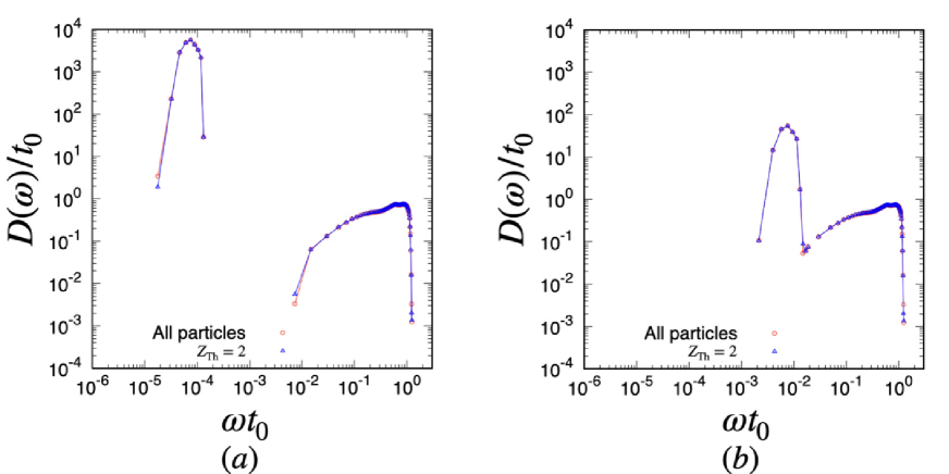
Refer to caption
Figure 13: Double logarithmic plots of Dโ€‹(ฯ‰)๐ท๐œ”D(\omega) with (red circles) and without (blue triangles by using ZTh=2subscript๐‘Th2Z_{\textrm{Th}}=2) rattlers against ฯ‰โ€‹t0๐œ”subscript๐‘ก0\omega t_{0} for ฯ•=0.90italic-ฯ•0.90\phi=0.90 at (a) kT/kN=1.0ร—10โˆ’8subscript๐‘˜๐‘‡subscript๐‘˜๐‘1.0superscript108k_{T}/k_{N}=1.0\times 10^{-8} and (b) kT/kN=1.0ร—10โˆ’4subscript๐‘˜๐‘‡subscript๐‘˜๐‘1.0superscript104k_{T}/k_{N}=1.0\times 10^{-4}. These figures are based on numerical results for N=4096๐‘4096N=4096.

E.2 Participation ratio

In this subsection, to clarify whether the mode at ฯ‰nsubscript๐œ”๐‘›\omega_{n} is localized or spread to the whole system, we introduce a participation ratio pnsubscript๐‘๐‘›p_{n} Yunker11 ; Shiraishi19

pn:=(โˆ‘i=1N|๐‘นn,i|2)2Nโ€‹โˆ‘i=1N|๐‘นn,i|4.assignsubscript๐‘๐‘›superscriptsuperscriptsubscript๐‘–1๐‘superscriptsubscript๐‘น๐‘›๐‘–22๐‘superscriptsubscript๐‘–1๐‘superscriptsubscript๐‘น๐‘›๐‘–4\displaystyle p_{n}:=\frac{\left(\sum_{i=1}^{N}|\bm{R}_{n,i}|^{2}\right)^{2}}{N\sum_{i=1}^{N}|\bm{R}_{n,i}|^{4}}. (64)

We plot pโ€‹(ฯ‰)๐‘๐œ”p(\omega) defined as

pโ€‹(ฯ‰):=โˆ‘nโ€ฒโŸจpnโ€‹ฮดโ€‹(ฯ‰โˆ’ฯ‰n)โŸฉโˆ‘nโ€ฒโŸจฮดโ€‹(ฯ‰โˆ’ฯ‰n)โŸฉassign๐‘๐œ”superscriptsubscript๐‘›โ€ฒdelimited-โŸจโŸฉsubscript๐‘๐‘›๐›ฟ๐œ”subscript๐œ”๐‘›superscriptsubscript๐‘›โ€ฒdelimited-โŸจโŸฉ๐›ฟ๐œ”subscript๐œ”๐‘›\displaystyle p(\omega):=\frac{\sum_{n}\nolimits^{\prime}\langle p_{n}\delta(\omega-\omega_{n})\rangle}{\sum_{n}\nolimits^{\prime}\langle\delta(\omega-\omega_{n})\rangle} (65)

against ฯ‰โ€‹t0๐œ”subscript๐‘ก0\omega t_{0} for ฯ•=0.90italic-ฯ•0.90\phi=0.90 in Fig. 14. Note that pโ€‹(ฯ‰)๐‘๐œ”p(\omega) are set to be zero if there is no right eigenvalue in the region (ฯ‰(s)<ฯ‰<ฯ‰(s+1))superscript๐œ”๐‘ ๐œ”superscript๐œ”๐‘ 1(\omega^{(s)}<\omega<\omega^{(s+1)}).

Refer to caption
Figure 14: Double logarithmic plots of pโ€‹(ฯ‰)๐‘๐œ”p(\omega) for ฯ•=0.90italic-ฯ•0.90\phi=0.90 against ฯ‰โ€‹t0๐œ”subscript๐‘ก0\omega t_{0} at (a) kT/kN=1.0ร—10โˆ’8subscript๐‘˜๐‘‡subscript๐‘˜๐‘1.0superscript108k_{T}/k_{N}=1.0\times 10^{-8} and (b) kT/kN=1.0ร—10โˆ’4subscript๐‘˜๐‘‡subscript๐‘˜๐‘1.0superscript104k_{T}/k_{N}=1.0\times 10^{-4}, where the guide line is 1/N1๐‘1/N. These figures are based on numerical results for N=4096๐‘4096N=4096.

Figure 14 shows that the modes at ฯ‰โ€‹t0โ‰ˆ10โˆ’5๐œ”subscript๐‘ก0superscript105\omega t_{0}\approx 10^{-5} in Fig. 14 (a) and at ฯ‰โ€‹t0โ‰ˆ10โˆ’3๐œ”subscript๐‘ก0superscript103\omega t_{0}\approx 10^{-3} in Fig. 14 (b) are nearly equal to pโ‰ˆ1/N๐‘1๐‘p\approx 1/N. Recalling that those modes consist of the rattler, we conclude that the contribution of the rattler is localized. In the middle range of ฯ‰๐œ”\omega in Fig. 14, there is an isolated band which shifts to the large ฯ‰๐œ”\omega as kT/kNsubscript๐‘˜๐‘‡subscript๐‘˜๐‘k_{T}/k_{N} increases with keeping its shape which can be seen in the main text.

Appendix F Explicit results of ๐’ฅNsubscript๐’ฅ๐‘\mathcal{J}_{N} and ๐’ฅTsubscript๐’ฅ๐‘‡\mathcal{J}_{T}

In this Appendix, we have written down the explicit results of ๐’ฅNsubscript๐’ฅ๐‘\mathcal{J}_{N} and ๐’ฅTsubscript๐’ฅ๐‘‡\mathcal{J}_{T}. From the results for the derivative of F~iฮฑsuperscriptsubscript~๐น๐‘–๐›ผ\tilde{F}_{i}^{\alpha} in Appendix D , the non-diagonal block elements ๐’ฅN,iโ€‹jฮฑโ€‹ฮฒ,๐’ฅT,iโ€‹jฮฑโ€‹ฮฒโ€‹(iโ‰ j)superscriptsubscript๐’ฅ๐‘๐‘–๐‘—๐›ผ๐›ฝsuperscriptsubscript๐’ฅ๐‘‡๐‘–๐‘—๐›ผ๐›ฝ๐‘–๐‘—\mathcal{J}_{N,ij}^{\alpha\beta},\mathcal{J}_{T,ij}^{\alpha\beta}(i\neq j) are given by

๐’ฅN,iโ€‹jxโ€‹xsuperscriptsubscript๐’ฅ๐‘๐‘–๐‘—๐‘ฅ๐‘ฅ\displaystyle\mathcal{J}_{N,ij}^{xx} =kNโ€‹ฮพiโ€‹j,N3/2riโ€‹jโˆ’kNโ€‹[32+ฮพiโ€‹j,Nriโ€‹j]โ€‹ฮพiโ€‹j,N1/2โ€‹(niโ€‹jx)2,absentsubscript๐‘˜๐‘superscriptsubscript๐œ‰๐‘–๐‘—๐‘32subscript๐‘Ÿ๐‘–๐‘—subscript๐‘˜๐‘delimited-[]32subscript๐œ‰๐‘–๐‘—๐‘subscript๐‘Ÿ๐‘–๐‘—superscriptsubscript๐œ‰๐‘–๐‘—๐‘12superscriptsuperscriptsubscript๐‘›๐‘–๐‘—๐‘ฅ2\displaystyle=k_{N}\frac{\xi_{ij,N}^{3/2}}{r_{ij}}-k_{N}\left[\frac{3}{2}+\frac{\xi_{ij,N}}{r_{ij}}\right]\xi_{ij,N}^{1/2}(n_{ij}^{x})^{2}, (66)
๐’ฅT,iโ€‹jxโ€‹xsuperscriptsubscript๐’ฅ๐‘‡๐‘–๐‘—๐‘ฅ๐‘ฅ\displaystyle\mathcal{J}_{T,ij}^{xx} โˆ’kTโ€‹ฮพiโ€‹j,N1/2โ€‹(niโ€‹jy)2+12โ€‹kTโ€‹ฮพiโ€‹j,Nโˆ’1/2โ€‹ฮพiโ€‹j,Tโ€‹niโ€‹jxโ€‹tiโ€‹jx,subscript๐‘˜๐‘‡superscriptsubscript๐œ‰๐‘–๐‘—๐‘12superscriptsuperscriptsubscript๐‘›๐‘–๐‘—๐‘ฆ212subscript๐‘˜๐‘‡superscriptsubscript๐œ‰๐‘–๐‘—๐‘12subscript๐œ‰๐‘–๐‘—๐‘‡superscriptsubscript๐‘›๐‘–๐‘—๐‘ฅsuperscriptsubscript๐‘ก๐‘–๐‘—๐‘ฅ\displaystyle-k_{T}\xi_{ij,N}^{1/2}(n_{ij}^{y})^{2}+\frac{1}{2}k_{T}\xi_{ij,N}^{-1/2}\xi_{ij,T}n_{ij}^{x}t_{ij}^{x}, (67)
๐’ฅN,iโ€‹jxโ€‹ysuperscriptsubscript๐’ฅ๐‘๐‘–๐‘—๐‘ฅ๐‘ฆ\displaystyle\mathcal{J}_{N,ij}^{xy} =โˆ’kNโ€‹[32+ฮพiโ€‹j,Nriโ€‹j]โ€‹ฮพiโ€‹j,N1/2โ€‹niโ€‹jxโ€‹niโ€‹jy,absentsubscript๐‘˜๐‘delimited-[]32subscript๐œ‰๐‘–๐‘—๐‘subscript๐‘Ÿ๐‘–๐‘—superscriptsubscript๐œ‰๐‘–๐‘—๐‘12superscriptsubscript๐‘›๐‘–๐‘—๐‘ฅsuperscriptsubscript๐‘›๐‘–๐‘—๐‘ฆ\displaystyle=-k_{N}\left[\frac{3}{2}+\frac{\xi_{ij,N}}{r_{ij}}\right]\xi_{ij,N}^{1/2}n_{ij}^{x}n_{ij}^{y}, (68)
๐’ฅT,iโ€‹jxโ€‹ysuperscriptsubscript๐’ฅ๐‘‡๐‘–๐‘—๐‘ฅ๐‘ฆ\displaystyle\mathcal{J}_{T,ij}^{xy} =kTโ€‹ฮพiโ€‹j,N1/2โ€‹niโ€‹jxโ€‹niโ€‹jy+12โ€‹kTโ€‹ฮพiโ€‹j,Nโˆ’1/2โ€‹ฮพiโ€‹j,Tโ€‹niโ€‹jxโ€‹tiโ€‹jy,absentsubscript๐‘˜๐‘‡superscriptsubscript๐œ‰๐‘–๐‘—๐‘12superscriptsubscript๐‘›๐‘–๐‘—๐‘ฅsuperscriptsubscript๐‘›๐‘–๐‘—๐‘ฆ12subscript๐‘˜๐‘‡superscriptsubscript๐œ‰๐‘–๐‘—๐‘12subscript๐œ‰๐‘–๐‘—๐‘‡superscriptsubscript๐‘›๐‘–๐‘—๐‘ฅsuperscriptsubscript๐‘ก๐‘–๐‘—๐‘ฆ\displaystyle=k_{T}\xi_{ij,N}^{1/2}n_{ij}^{x}n_{ij}^{y}+\frac{1}{2}k_{T}\xi_{ij,N}^{-1/2}\xi_{ij,T}n_{ij}^{x}t_{ij}^{y}, (69)
๐’ฅN,iโ€‹jxโ€‹โ„“superscriptsubscript๐’ฅ๐‘๐‘–๐‘—๐‘ฅโ„“\displaystyle\mathcal{J}_{N,ij}^{x\ell} =0,absent0\displaystyle=0, (70)
๐’ฅT,iโ€‹jxโ€‹โ„“superscriptsubscript๐’ฅ๐‘‡๐‘–๐‘—๐‘ฅโ„“\displaystyle\mathcal{J}_{T,ij}^{x\ell} =kTโ€‹ฮพiโ€‹j,N1/2โ€‹niโ€‹jy+12โ€‹kTโ€‹ฮพiโ€‹j,Nโˆ’1/2โ€‹ฮพiโ€‹j,Tโ€‹niโ€‹jxโ€‹(niโ€‹jxโ€‹tiโ€‹jyโˆ’niโ€‹jyโ€‹tiโ€‹jx),absentsubscript๐‘˜๐‘‡superscriptsubscript๐œ‰๐‘–๐‘—๐‘12superscriptsubscript๐‘›๐‘–๐‘—๐‘ฆ12subscript๐‘˜๐‘‡superscriptsubscript๐œ‰๐‘–๐‘—๐‘12subscript๐œ‰๐‘–๐‘—๐‘‡superscriptsubscript๐‘›๐‘–๐‘—๐‘ฅsuperscriptsubscript๐‘›๐‘–๐‘—๐‘ฅsuperscriptsubscript๐‘ก๐‘–๐‘—๐‘ฆsuperscriptsubscript๐‘›๐‘–๐‘—๐‘ฆsuperscriptsubscript๐‘ก๐‘–๐‘—๐‘ฅ\displaystyle=k_{T}\xi_{ij,N}^{1/2}n_{ij}^{y}+\frac{1}{2}k_{T}\xi_{ij,N}^{-1/2}\xi_{ij,T}n_{ij}^{x}(n_{ij}^{x}t_{ij}^{y}-n_{ij}^{y}t_{ij}^{x}), (71)
๐’ฅN,iโ€‹jyโ€‹xsuperscriptsubscript๐’ฅ๐‘๐‘–๐‘—๐‘ฆ๐‘ฅ\displaystyle\mathcal{J}_{N,ij}^{yx} =โˆ’kNโ€‹[32+ฮพiโ€‹j,Nriโ€‹j]โ€‹ฮพiโ€‹j,N1/2โ€‹niโ€‹jxโ€‹niโ€‹jy,absentsubscript๐‘˜๐‘delimited-[]32subscript๐œ‰๐‘–๐‘—๐‘subscript๐‘Ÿ๐‘–๐‘—superscriptsubscript๐œ‰๐‘–๐‘—๐‘12superscriptsubscript๐‘›๐‘–๐‘—๐‘ฅsuperscriptsubscript๐‘›๐‘–๐‘—๐‘ฆ\displaystyle=-k_{N}\left[\frac{3}{2}+\frac{\xi_{ij,N}}{r_{ij}}\right]\xi_{ij,N}^{1/2}n_{ij}^{x}n_{ij}^{y}, (72)
๐’ฅT,iโ€‹jyโ€‹xsuperscriptsubscript๐’ฅ๐‘‡๐‘–๐‘—๐‘ฆ๐‘ฅ\displaystyle\mathcal{J}_{T,ij}^{yx} =kTโ€‹ฮพiโ€‹j,N1/2โ€‹niโ€‹jxโ€‹niโ€‹jy+12โ€‹kTโ€‹ฮพiโ€‹j,Nโˆ’1/2โ€‹ฮพiโ€‹j,Tโ€‹niโ€‹jyโ€‹tiโ€‹jx,absentsubscript๐‘˜๐‘‡superscriptsubscript๐œ‰๐‘–๐‘—๐‘12superscriptsubscript๐‘›๐‘–๐‘—๐‘ฅsuperscriptsubscript๐‘›๐‘–๐‘—๐‘ฆ12subscript๐‘˜๐‘‡superscriptsubscript๐œ‰๐‘–๐‘—๐‘12subscript๐œ‰๐‘–๐‘—๐‘‡superscriptsubscript๐‘›๐‘–๐‘—๐‘ฆsuperscriptsubscript๐‘ก๐‘–๐‘—๐‘ฅ\displaystyle=k_{T}\xi_{ij,N}^{1/2}n_{ij}^{x}n_{ij}^{y}+\frac{1}{2}k_{T}\xi_{ij,N}^{-1/2}\xi_{ij,T}n_{ij}^{y}t_{ij}^{x}, (73)
๐’ฅN,iโ€‹jyโ€‹ysuperscriptsubscript๐’ฅ๐‘๐‘–๐‘—๐‘ฆ๐‘ฆ\displaystyle\mathcal{J}_{N,ij}^{yy} =kNโ€‹ฮพiโ€‹j,N3/2riโ€‹jโˆ’kNโ€‹[32+ฮพiโ€‹j,Nriโ€‹j]โ€‹ฮพiโ€‹j,N1/2โ€‹(niโ€‹jy)2,absentsubscript๐‘˜๐‘superscriptsubscript๐œ‰๐‘–๐‘—๐‘32subscript๐‘Ÿ๐‘–๐‘—subscript๐‘˜๐‘delimited-[]32subscript๐œ‰๐‘–๐‘—๐‘subscript๐‘Ÿ๐‘–๐‘—superscriptsubscript๐œ‰๐‘–๐‘—๐‘12superscriptsuperscriptsubscript๐‘›๐‘–๐‘—๐‘ฆ2\displaystyle=k_{N}\frac{\xi_{ij,N}^{3/2}}{r_{ij}}-k_{N}\left[\frac{3}{2}+\frac{\xi_{ij,N}}{r_{ij}}\right]\xi_{ij,N}^{1/2}(n_{ij}^{y})^{2}, (74)
๐’ฅT,iโ€‹jyโ€‹ysuperscriptsubscript๐’ฅ๐‘‡๐‘–๐‘—๐‘ฆ๐‘ฆ\displaystyle\mathcal{J}_{T,ij}^{yy} =โˆ’kTโ€‹ฮพiโ€‹j,N1/2โ€‹(niโ€‹jx)2+12โ€‹kTโ€‹ฮพiโ€‹j,Nโˆ’1/2โ€‹ฮพiโ€‹j,Tโ€‹niโ€‹jyโ€‹tiโ€‹jy,absentsubscript๐‘˜๐‘‡superscriptsubscript๐œ‰๐‘–๐‘—๐‘12superscriptsuperscriptsubscript๐‘›๐‘–๐‘—๐‘ฅ212subscript๐‘˜๐‘‡superscriptsubscript๐œ‰๐‘–๐‘—๐‘12subscript๐œ‰๐‘–๐‘—๐‘‡superscriptsubscript๐‘›๐‘–๐‘—๐‘ฆsuperscriptsubscript๐‘ก๐‘–๐‘—๐‘ฆ\displaystyle=-k_{T}\xi_{ij,N}^{1/2}(n_{ij}^{x})^{2}+\frac{1}{2}k_{T}\xi_{ij,N}^{-1/2}\xi_{ij,T}n_{ij}^{y}t_{ij}^{y}, (75)
๐’ฅN,iโ€‹jyโ€‹โ„“superscriptsubscript๐’ฅ๐‘๐‘–๐‘—๐‘ฆโ„“\displaystyle\mathcal{J}_{N,ij}^{y\ell} =0,absent0\displaystyle=0, (76)
๐’ฅT,iโ€‹jyโ€‹โ„“superscriptsubscript๐’ฅ๐‘‡๐‘–๐‘—๐‘ฆโ„“\displaystyle\mathcal{J}_{T,ij}^{y\ell} =โˆ’kTโ€‹ฮพiโ€‹j,N1/2โ€‹niโ€‹jx+12โ€‹kTโ€‹ฮพiโ€‹j,Nโˆ’1/2โ€‹ฮพiโ€‹j,Tโ€‹niโ€‹jyโ€‹(niโ€‹jxโ€‹tiโ€‹jyโˆ’niโ€‹jyโ€‹tiโ€‹jx),absentsubscript๐‘˜๐‘‡superscriptsubscript๐œ‰๐‘–๐‘—๐‘12superscriptsubscript๐‘›๐‘–๐‘—๐‘ฅ12subscript๐‘˜๐‘‡superscriptsubscript๐œ‰๐‘–๐‘—๐‘12subscript๐œ‰๐‘–๐‘—๐‘‡superscriptsubscript๐‘›๐‘–๐‘—๐‘ฆsuperscriptsubscript๐‘›๐‘–๐‘—๐‘ฅsuperscriptsubscript๐‘ก๐‘–๐‘—๐‘ฆsuperscriptsubscript๐‘›๐‘–๐‘—๐‘ฆsuperscriptsubscript๐‘ก๐‘–๐‘—๐‘ฅ\displaystyle=-k_{T}\xi_{ij,N}^{1/2}n_{ij}^{x}+\frac{1}{2}k_{T}\xi_{ij,N}^{-1/2}\xi_{ij,T}n_{ij}^{y}(n_{ij}^{x}t_{ij}^{y}-n_{ij}^{y}t_{ij}^{x}), (77)
๐’ฅN,iโ€‹jโ„“โ€‹xsuperscriptsubscript๐’ฅ๐‘๐‘–๐‘—โ„“๐‘ฅ\displaystyle\mathcal{J}_{N,ij}^{\ell x} =0,absent0\displaystyle=0, (78)
๐’ฅT,iโ€‹jโ„“โ€‹xsuperscriptsubscript๐’ฅ๐‘‡๐‘–๐‘—โ„“๐‘ฅ\displaystyle\mathcal{J}_{T,ij}^{\ell x} =โˆ’kTโ€‹ฮพiโ€‹j,N1/2โ€‹niโ€‹jy,absentsubscript๐‘˜๐‘‡superscriptsubscript๐œ‰๐‘–๐‘—๐‘12superscriptsubscript๐‘›๐‘–๐‘—๐‘ฆ\displaystyle=-k_{T}\xi_{ij,N}^{1/2}n_{ij}^{y}, (79)
๐’ฅN,iโ€‹jโ„“โ€‹ysuperscriptsubscript๐’ฅ๐‘๐‘–๐‘—โ„“๐‘ฆ\displaystyle\mathcal{J}_{N,ij}^{\ell y} =0,absent0\displaystyle=0, (80)
๐’ฅT,iโ€‹jโ„“โ€‹ysuperscriptsubscript๐’ฅ๐‘‡๐‘–๐‘—โ„“๐‘ฆ\displaystyle\mathcal{J}_{T,ij}^{\ell y} =kTโ€‹ฮพiโ€‹j,N1/2โ€‹niโ€‹jx,absentsubscript๐‘˜๐‘‡superscriptsubscript๐œ‰๐‘–๐‘—๐‘12superscriptsubscript๐‘›๐‘–๐‘—๐‘ฅ\displaystyle=k_{T}\xi_{ij,N}^{1/2}n_{ij}^{x}, (81)
๐’ฅN,iโ€‹jโ„“โ€‹โ„“superscriptsubscript๐’ฅ๐‘๐‘–๐‘—โ„“โ„“\displaystyle\mathcal{J}_{N,ij}^{\ell\ell} =0,absent0\displaystyle=0, (82)
๐’ฅT,iโ€‹jโ„“โ€‹โ„“superscriptsubscript๐’ฅ๐‘‡๐‘–๐‘—โ„“โ„“\displaystyle\mathcal{J}_{T,ij}^{\ell\ell} =kTโ€‹ฮพiโ€‹j,N1/2.absentsubscript๐‘˜๐‘‡superscriptsubscript๐œ‰๐‘–๐‘—๐‘12\displaystyle=k_{T}\xi_{ij,N}^{1/2}. (83)

Similarly, the diagonal block elements ๐’ฅN,iโ€‹jฮฑโ€‹ฮฒ,๐’ฅT,iโ€‹jฮฑโ€‹ฮฒโ€‹(i=j)superscriptsubscript๐’ฅ๐‘๐‘–๐‘—๐›ผ๐›ฝsuperscriptsubscript๐’ฅ๐‘‡๐‘–๐‘—๐›ผ๐›ฝ๐‘–๐‘—\mathcal{J}_{N,ij}^{\alpha\beta},\mathcal{J}_{T,ij}^{\alpha\beta}(i=j) are given by

๐’ฅN,iโ€‹ixโ€‹xsuperscriptsubscript๐’ฅ๐‘๐‘–๐‘–๐‘ฅ๐‘ฅ\displaystyle\mathcal{J}_{N,ii}^{xx} =โˆ’โˆ‘jโ‰ i{kNโ€‹ฮพiโ€‹j,N3/2riโ€‹jโˆ’kNโ€‹[32+ฮพiโ€‹j,Nriโ€‹j]โ€‹ฮพiโ€‹j,N1/2โ€‹(niโ€‹jx)2},absentsubscript๐‘—๐‘–subscript๐‘˜๐‘superscriptsubscript๐œ‰๐‘–๐‘—๐‘32subscript๐‘Ÿ๐‘–๐‘—subscript๐‘˜๐‘delimited-[]32subscript๐œ‰๐‘–๐‘—๐‘subscript๐‘Ÿ๐‘–๐‘—superscriptsubscript๐œ‰๐‘–๐‘—๐‘12superscriptsuperscriptsubscript๐‘›๐‘–๐‘—๐‘ฅ2\displaystyle=-\sum_{j\neq i}\left\{k_{N}\frac{\xi_{ij,N}^{3/2}}{r_{ij}}-k_{N}\left[\frac{3}{2}+\frac{\xi_{ij,N}}{r_{ij}}\right]\xi_{ij,N}^{1/2}(n_{ij}^{x})^{2}\right\}, (84)
๐’ฅT,iโ€‹ixโ€‹xsuperscriptsubscript๐’ฅ๐‘‡๐‘–๐‘–๐‘ฅ๐‘ฅ\displaystyle\mathcal{J}_{T,ii}^{xx} =โˆ’โˆ‘jโ‰ i{โˆ’kTโ€‹ฮพiโ€‹j,N1/2โ€‹(niโ€‹jy)2+12โ€‹kTโ€‹ฮพiโ€‹j,Nโˆ’1/2โ€‹ฮพiโ€‹j,Tโ€‹niโ€‹jxโ€‹tiโ€‹jx},absentsubscript๐‘—๐‘–subscript๐‘˜๐‘‡superscriptsubscript๐œ‰๐‘–๐‘—๐‘12superscriptsuperscriptsubscript๐‘›๐‘–๐‘—๐‘ฆ212subscript๐‘˜๐‘‡superscriptsubscript๐œ‰๐‘–๐‘—๐‘12subscript๐œ‰๐‘–๐‘—๐‘‡superscriptsubscript๐‘›๐‘–๐‘—๐‘ฅsuperscriptsubscript๐‘ก๐‘–๐‘—๐‘ฅ\displaystyle=-\sum_{j\neq i}\left\{-k_{T}\xi_{ij,N}^{1/2}(n_{ij}^{y})^{2}+\frac{1}{2}k_{T}\xi_{ij,N}^{-1/2}\xi_{ij,T}n_{ij}^{x}t_{ij}^{x}\right\}, (85)
๐’ฅN,iโ€‹ixโ€‹ysuperscriptsubscript๐’ฅ๐‘๐‘–๐‘–๐‘ฅ๐‘ฆ\displaystyle\mathcal{J}_{N,ii}^{xy} =โˆ’โˆ‘jโ‰ i{โˆ’kNโ€‹[32+ฮพiโ€‹j,Nriโ€‹j]โ€‹ฮพiโ€‹j,N1/2โ€‹niโ€‹jxโ€‹niโ€‹jy},absentsubscript๐‘—๐‘–subscript๐‘˜๐‘delimited-[]32subscript๐œ‰๐‘–๐‘—๐‘subscript๐‘Ÿ๐‘–๐‘—superscriptsubscript๐œ‰๐‘–๐‘—๐‘12superscriptsubscript๐‘›๐‘–๐‘—๐‘ฅsuperscriptsubscript๐‘›๐‘–๐‘—๐‘ฆ\displaystyle=-\sum_{j\neq i}\left\{-k_{N}\left[\frac{3}{2}+\frac{\xi_{ij,N}}{r_{ij}}\right]\xi_{ij,N}^{1/2}n_{ij}^{x}n_{ij}^{y}\right\}, (86)
๐’ฅT,iโ€‹ixโ€‹ysuperscriptsubscript๐’ฅ๐‘‡๐‘–๐‘–๐‘ฅ๐‘ฆ\displaystyle\mathcal{J}_{T,ii}^{xy} =โˆ’โˆ‘jโ‰ i{kTโ€‹ฮพiโ€‹j,N1/2โ€‹niโ€‹jxโ€‹niโ€‹jy+12โ€‹kTโ€‹ฮพiโ€‹j,Nโˆ’1/2โ€‹ฮพiโ€‹j,Tโ€‹niโ€‹jxโ€‹tiโ€‹jy},absentsubscript๐‘—๐‘–subscript๐‘˜๐‘‡superscriptsubscript๐œ‰๐‘–๐‘—๐‘12superscriptsubscript๐‘›๐‘–๐‘—๐‘ฅsuperscriptsubscript๐‘›๐‘–๐‘—๐‘ฆ12subscript๐‘˜๐‘‡superscriptsubscript๐œ‰๐‘–๐‘—๐‘12subscript๐œ‰๐‘–๐‘—๐‘‡superscriptsubscript๐‘›๐‘–๐‘—๐‘ฅsuperscriptsubscript๐‘ก๐‘–๐‘—๐‘ฆ\displaystyle=-\sum_{j\neq i}\left\{k_{T}\xi_{ij,N}^{1/2}n_{ij}^{x}n_{ij}^{y}+\frac{1}{2}k_{T}\xi_{ij,N}^{-1/2}\xi_{ij,T}n_{ij}^{x}t_{ij}^{y}\right\}, (87)
๐’ฅN,iโ€‹ixโ€‹โ„“superscriptsubscript๐’ฅ๐‘๐‘–๐‘–๐‘ฅโ„“\displaystyle\mathcal{J}_{N,ii}^{x\ell} =0,absent0\displaystyle=0, (88)
๐’ฅT,iโ€‹ixโ€‹โ„“superscriptsubscript๐’ฅ๐‘‡๐‘–๐‘–๐‘ฅโ„“\displaystyle\mathcal{J}_{T,ii}^{x\ell} =โˆ‘jโ‰ i{kTโ€‹ฮพiโ€‹j,N1/2โ€‹niโ€‹jy+12โ€‹ฮพiโ€‹j,Nโˆ’1/2โ€‹ฮพiโ€‹j,Tโ€‹niโ€‹jxโ€‹(niโ€‹jxโ€‹tiโ€‹jyโˆ’niโ€‹jyโ€‹tiโ€‹jx)},absentsubscript๐‘—๐‘–subscript๐‘˜๐‘‡superscriptsubscript๐œ‰๐‘–๐‘—๐‘12superscriptsubscript๐‘›๐‘–๐‘—๐‘ฆ12superscriptsubscript๐œ‰๐‘–๐‘—๐‘12subscript๐œ‰๐‘–๐‘—๐‘‡superscriptsubscript๐‘›๐‘–๐‘—๐‘ฅsuperscriptsubscript๐‘›๐‘–๐‘—๐‘ฅsuperscriptsubscript๐‘ก๐‘–๐‘—๐‘ฆsuperscriptsubscript๐‘›๐‘–๐‘—๐‘ฆsuperscriptsubscript๐‘ก๐‘–๐‘—๐‘ฅ\displaystyle=\sum_{j\neq i}\left\{k_{T}\xi_{ij,N}^{1/2}n_{ij}^{y}+\frac{1}{2}\xi_{ij,N}^{-1/2}\xi_{ij,T}n_{ij}^{x}(n_{ij}^{x}t_{ij}^{y}-n_{ij}^{y}t_{ij}^{x})\right\}, (89)
๐’ฅN,iโ€‹iyโ€‹xsuperscriptsubscript๐’ฅ๐‘๐‘–๐‘–๐‘ฆ๐‘ฅ\displaystyle\mathcal{J}_{N,ii}^{yx} =โˆ’โˆ‘jโ‰ i{โˆ’kNโ€‹[32+ฮพiโ€‹j,Nriโ€‹j]โ€‹ฮพiโ€‹j,N1/2โ€‹niโ€‹jxโ€‹niโ€‹jy},absentsubscript๐‘—๐‘–subscript๐‘˜๐‘delimited-[]32subscript๐œ‰๐‘–๐‘—๐‘subscript๐‘Ÿ๐‘–๐‘—superscriptsubscript๐œ‰๐‘–๐‘—๐‘12superscriptsubscript๐‘›๐‘–๐‘—๐‘ฅsuperscriptsubscript๐‘›๐‘–๐‘—๐‘ฆ\displaystyle=-\sum_{j\neq i}\left\{-k_{N}\left[\frac{3}{2}+\frac{\xi_{ij,N}}{r_{ij}}\right]\xi_{ij,N}^{1/2}n_{ij}^{x}n_{ij}^{y}\right\}, (90)
๐’ฅT,iโ€‹iyโ€‹xsuperscriptsubscript๐’ฅ๐‘‡๐‘–๐‘–๐‘ฆ๐‘ฅ\displaystyle\mathcal{J}_{T,ii}^{yx} =โˆ’โˆ‘jโ‰ i{kTโ€‹ฮพiโ€‹j,N1/2โ€‹niโ€‹jxโ€‹niโ€‹jy+12โ€‹kTโ€‹ฮพiโ€‹j,Nโˆ’1/2โ€‹ฮพiโ€‹j,Tโ€‹niโ€‹jyโ€‹tiโ€‹jx},absentsubscript๐‘—๐‘–subscript๐‘˜๐‘‡superscriptsubscript๐œ‰๐‘–๐‘—๐‘12superscriptsubscript๐‘›๐‘–๐‘—๐‘ฅsuperscriptsubscript๐‘›๐‘–๐‘—๐‘ฆ12subscript๐‘˜๐‘‡superscriptsubscript๐œ‰๐‘–๐‘—๐‘12subscript๐œ‰๐‘–๐‘—๐‘‡superscriptsubscript๐‘›๐‘–๐‘—๐‘ฆsuperscriptsubscript๐‘ก๐‘–๐‘—๐‘ฅ\displaystyle=-\sum_{j\neq i}\left\{k_{T}\xi_{ij,N}^{1/2}n_{ij}^{x}n_{ij}^{y}+\frac{1}{2}k_{T}\xi_{ij,N}^{-1/2}\xi_{ij,T}n_{ij}^{y}t_{ij}^{x}\right\}, (91)
๐’ฅN,iโ€‹iyโ€‹ysuperscriptsubscript๐’ฅ๐‘๐‘–๐‘–๐‘ฆ๐‘ฆ\displaystyle\mathcal{J}_{N,ii}^{yy} =โˆ’โˆ‘jโ‰ i{kNโ€‹ฮพiโ€‹j,N3/2riโ€‹jโˆ’kNโ€‹[32+ฮพiโ€‹j,Nriโ€‹j]โ€‹ฮพiโ€‹j,N1/2โ€‹(niโ€‹jy)2},absentsubscript๐‘—๐‘–subscript๐‘˜๐‘superscriptsubscript๐œ‰๐‘–๐‘—๐‘32subscript๐‘Ÿ๐‘–๐‘—subscript๐‘˜๐‘delimited-[]32subscript๐œ‰๐‘–๐‘—๐‘subscript๐‘Ÿ๐‘–๐‘—superscriptsubscript๐œ‰๐‘–๐‘—๐‘12superscriptsuperscriptsubscript๐‘›๐‘–๐‘—๐‘ฆ2\displaystyle=-\sum_{j\neq i}\left\{k_{N}\frac{\xi_{ij,N}^{3/2}}{r_{ij}}-k_{N}\left[\frac{3}{2}+\frac{\xi_{ij,N}}{r_{ij}}\right]\xi_{ij,N}^{1/2}(n_{ij}^{y})^{2}\right\}, (92)
๐’ฅT,iโ€‹iyโ€‹ysuperscriptsubscript๐’ฅ๐‘‡๐‘–๐‘–๐‘ฆ๐‘ฆ\displaystyle\mathcal{J}_{T,ii}^{yy} =โˆ’โˆ‘jโ‰ i{โˆ’kTโ€‹ฮพiโ€‹j,N1/2โ€‹(niโ€‹jx)2+12โ€‹kTโ€‹ฮพiโ€‹j,Nโˆ’1/2โ€‹ฮพiโ€‹j,Tโ€‹niโ€‹jyโ€‹tiโ€‹jy},absentsubscript๐‘—๐‘–subscript๐‘˜๐‘‡superscriptsubscript๐œ‰๐‘–๐‘—๐‘12superscriptsuperscriptsubscript๐‘›๐‘–๐‘—๐‘ฅ212subscript๐‘˜๐‘‡superscriptsubscript๐œ‰๐‘–๐‘—๐‘12subscript๐œ‰๐‘–๐‘—๐‘‡superscriptsubscript๐‘›๐‘–๐‘—๐‘ฆsuperscriptsubscript๐‘ก๐‘–๐‘—๐‘ฆ\displaystyle=-\sum_{j\neq i}\left\{-k_{T}\xi_{ij,N}^{1/2}(n_{ij}^{x})^{2}+\frac{1}{2}k_{T}\xi_{ij,N}^{-1/2}\xi_{ij,T}n_{ij}^{y}t_{ij}^{y}\right\}, (93)
๐’ฅN,iโ€‹iyโ€‹ysuperscriptsubscript๐’ฅ๐‘๐‘–๐‘–๐‘ฆ๐‘ฆ\displaystyle\mathcal{J}_{N,ii}^{yy} =0,absent0\displaystyle=0, (94)
๐’ฅT,iโ€‹iyโ€‹โ„“superscriptsubscript๐’ฅ๐‘‡๐‘–๐‘–๐‘ฆโ„“\displaystyle\mathcal{J}_{T,ii}^{y\ell} =โˆ’โˆ‘jโ‰ i{kTโ€‹ฮพiโ€‹j,N1/2โ€‹niโ€‹jx+12โ€‹kTโ€‹ฮพiโ€‹j,Nโˆ’1/2โ€‹ฮพiโ€‹j,Tโ€‹niโ€‹jyโ€‹(niโ€‹jxโ€‹tiโ€‹jyโˆ’niโ€‹jyโ€‹tiโ€‹jx)},absentsubscript๐‘—๐‘–subscript๐‘˜๐‘‡superscriptsubscript๐œ‰๐‘–๐‘—๐‘12superscriptsubscript๐‘›๐‘–๐‘—๐‘ฅ12subscript๐‘˜๐‘‡superscriptsubscript๐œ‰๐‘–๐‘—๐‘12subscript๐œ‰๐‘–๐‘—๐‘‡superscriptsubscript๐‘›๐‘–๐‘—๐‘ฆsuperscriptsubscript๐‘›๐‘–๐‘—๐‘ฅsuperscriptsubscript๐‘ก๐‘–๐‘—๐‘ฆsuperscriptsubscript๐‘›๐‘–๐‘—๐‘ฆsuperscriptsubscript๐‘ก๐‘–๐‘—๐‘ฅ\displaystyle=-\sum_{j\neq i}\left\{k_{T}\xi_{ij,N}^{1/2}n_{ij}^{x}+\frac{1}{2}k_{T}\xi_{ij,N}^{-1/2}\xi_{ij,T}n_{ij}^{y}(n_{ij}^{x}t_{ij}^{y}-n_{ij}^{y}t_{ij}^{x})\right\}, (95)
๐’ฅN,iโ€‹iโ„“โ€‹xsuperscriptsubscript๐’ฅ๐‘๐‘–๐‘–โ„“๐‘ฅ\displaystyle\mathcal{J}_{N,ii}^{\ell x} =0,absent0\displaystyle=0, (96)
๐’ฅT,iโ€‹iโ„“โ€‹xsuperscriptsubscript๐’ฅ๐‘‡๐‘–๐‘–โ„“๐‘ฅ\displaystyle\mathcal{J}_{T,ii}^{\ell x} =โˆ‘jโ‰ ikTโ€‹ฮพiโ€‹j,N1/2โ€‹niโ€‹jy,absentsubscript๐‘—๐‘–subscript๐‘˜๐‘‡superscriptsubscript๐œ‰๐‘–๐‘—๐‘12superscriptsubscript๐‘›๐‘–๐‘—๐‘ฆ\displaystyle=\sum_{j\neq i}k_{T}\xi_{ij,N}^{1/2}n_{ij}^{y}, (97)
๐’ฅN,iโ€‹iโ„“โ€‹ysuperscriptsubscript๐’ฅ๐‘๐‘–๐‘–โ„“๐‘ฆ\displaystyle\mathcal{J}_{N,ii}^{\ell y} =0,absent0\displaystyle=0, (98)
๐’ฅT,iโ€‹iโ„“โ€‹ysuperscriptsubscript๐’ฅ๐‘‡๐‘–๐‘–โ„“๐‘ฆ\displaystyle\mathcal{J}_{T,ii}^{\ell y} =โˆ’โˆ‘jโ‰ ikTโ€‹ฮพiโ€‹j,N1/2โ€‹niโ€‹jx,absentsubscript๐‘—๐‘–subscript๐‘˜๐‘‡superscriptsubscript๐œ‰๐‘–๐‘—๐‘12superscriptsubscript๐‘›๐‘–๐‘—๐‘ฅ\displaystyle=-\sum_{j\neq i}k_{T}\xi_{ij,N}^{1/2}n_{ij}^{x}, (99)
๐’ฅN,iโ€‹iโ„“โ€‹โ„“superscriptsubscript๐’ฅ๐‘๐‘–๐‘–โ„“โ„“\displaystyle\mathcal{J}_{N,ii}^{\ell\ell} =0,absent0\displaystyle=0, (100)
๐’ฅT,iโ€‹iโ„“โ€‹โ„“superscriptsubscript๐’ฅ๐‘‡๐‘–๐‘–โ„“โ„“\displaystyle\mathcal{J}_{T,ii}^{\ell\ell} =โˆ‘jโ‰ ikTโ€‹ฮพiโ€‹j,N1/2.absentsubscript๐‘—๐‘–subscript๐‘˜๐‘‡superscriptsubscript๐œ‰๐‘–๐‘—๐‘12\displaystyle=\sum_{j\neq i}k_{T}\xi_{ij,N}^{1/2}. (101)

Note that the terms proportional to ฮพiโ€‹j,Tsubscript๐œ‰๐‘–๐‘—๐‘‡\xi_{ij,T} in ๐’ฅTsubscript๐’ฅ๐‘‡\mathcal{J}_{T} include the history-dependent tangential displacements which are ignored in the effective potential Somfai07 ; Henkes10 ; Liu21 .

Appendix G The detailed derivation of G๐บG in the Jacobian analysis

In this Appendix, we derive Eq. (38) that gives the rigidity. First, nonaffine displacements are expanded in terms of eigenfunctions of the Jacobian. Next, we express the rigidity as the eigenvalues and eigenfunctions of the Jacobian. Note that we adopt the abbreviation dโ€‹Aโ€‹(๐’’FBโ€‹(0))/dโ€‹ฮณ:=dโ€‹Aโ€‹(๐’’โ€‹(ฮณ))/dโ€‹ฮณ|๐’’โ€‹(ฮณ)=๐’’FBโ€‹(0)assign๐‘‘๐ดsuperscript๐’’FB0๐‘‘๐›พevaluated-at๐‘‘๐ด๐’’๐›พ๐‘‘๐›พ๐’’๐›พsuperscript๐’’FB0dA(\bm{q}^{\textrm{FB}}(0))/d\gamma:=dA(\bm{q}(\gamma))/d\gamma|_{\bm{q}(\gamma)=\bm{q}^{\textrm{FB}}(0)} in this Appendix.

G.1 Expansion for nonaffine displacements via eigenfunction of Jacobian

At FB state, F~iฮฑ/dโ€‹ฮณsuperscriptsubscript~๐น๐‘–๐›ผ๐‘‘๐›พ\tilde{F}_{i}^{\alpha}/d\gamma is expressed as

dโ€‹F~iฮฑdโ€‹ฮณ๐‘‘superscriptsubscript~๐น๐‘–๐›ผ๐‘‘๐›พ\displaystyle\frac{d\tilde{F}_{i}^{\alpha}}{d\gamma} =limฮ”โ€‹ฮณโ†’0F~iฮฑโ€‹(๐’’FBโ€‹(ฮ”โ€‹ฮณ))โˆ’F~iฮฑโ€‹(๐’’FBโ€‹(0))ฮ”โ€‹ฮณabsentsubscriptโ†’ฮ”๐›พ0superscriptsubscript~๐น๐‘–๐›ผsuperscript๐’’FBฮ”๐›พsuperscriptsubscript~๐น๐‘–๐›ผsuperscript๐’’FB0ฮ”๐›พ\displaystyle=\lim_{\Delta\gamma\to 0}\frac{\tilde{F}_{i}^{\alpha}(\bm{q}^{\textrm{FB}}(\Delta\gamma))-\tilde{F}_{i}^{\alpha}(\bm{q}^{\textrm{FB}}(0))}{\Delta\gamma}
=โˆ‘jโ‰ i[โˆ‚fiโ€‹jฮฑโˆ‚qixโ€‹yiโ€‹jโ€‹(๐’’FBโ€‹(0))+โˆ‘ฮถ=x,yโˆ‚fiโ€‹jฮฑโˆ‚riฮถโ€‹dโ€‹rฬŠiโ€‹jฮถโ€‹(๐’’FBโ€‹(0))dโ€‹ฮณ+โˆ‚fiโ€‹jฮฑโˆ‚โ„“iโ€‹(dโ€‹โ„“ฬŠiโ€‹(๐’’FBโ€‹(0))dโ€‹ฮณ+dโ€‹โ„“ฬŠjโ€‹(๐’’FBโ€‹(0))dโ€‹ฮณ)].absentsubscript๐‘—๐‘–delimited-[]superscriptsubscript๐‘“๐‘–๐‘—๐›ผsuperscriptsubscript๐‘ž๐‘–๐‘ฅsubscript๐‘ฆ๐‘–๐‘—superscript๐’’FB0subscript๐œ๐‘ฅ๐‘ฆsuperscriptsubscript๐‘“๐‘–๐‘—๐›ผsuperscriptsubscript๐‘Ÿ๐‘–๐œ๐‘‘superscriptsubscriptฬŠ๐‘Ÿ๐‘–๐‘—๐œsuperscript๐’’FB0๐‘‘๐›พsuperscriptsubscript๐‘“๐‘–๐‘—๐›ผsubscriptโ„“๐‘–๐‘‘subscriptฬŠโ„“๐‘–superscript๐’’FB0๐‘‘๐›พ๐‘‘subscriptฬŠโ„“๐‘—superscript๐’’FB0๐‘‘๐›พ\displaystyle=\sum_{j\neq i}\left[\frac{\partial f_{ij}^{\alpha}}{\partial q_{i}^{x}}y_{ij}(\bm{q}^{\textrm{FB}}(0))+\sum_{\zeta=x,y}\frac{\partial f_{ij}^{\alpha}}{\partial r_{i}^{\zeta}}\frac{d\mathring{r}_{ij}^{\zeta}(\bm{q}^{\textrm{FB}}(0))}{d\gamma}+\frac{\partial f_{ij}^{\alpha}}{\partial\ell_{i}}\left(\frac{d\mathring{\ell}_{i}(\bm{q}^{\textrm{FB}}(0))}{d\gamma}+\frac{d\mathring{\ell}_{j}(\bm{q}^{\textrm{FB}}(0))}{d\gamma}\right)\right]. (102)

Using the Jacobian, we rewrite Eq. (102) as

dโ€‹F~iฮฑdโ€‹ฮณ๐‘‘superscriptsubscript~๐น๐‘–๐›ผ๐‘‘๐›พ\displaystyle\frac{d\tilde{F}_{i}^{\alpha}}{d\gamma} =โˆ’โˆ‘jโ‰ i[๐’ฅjโ€‹iฮฑโ€‹xโ€‹yiโ€‹jโ€‹(๐’’FBโ€‹(0))+โˆ‘ฮถ=x,y๐’ฅjโ€‹iฮฑโ€‹ฮถโ€‹dโ€‹rฬŠiโ€‹jฮถโ€‹(๐’’FBโ€‹(0))dโ€‹ฮณ+๐’ฅjโ€‹iฮฑโ€‹โ„“โ€‹(dโ€‹โ„“ฬŠiโ€‹(๐’’FBโ€‹(0))dโ€‹ฮณ+dโ€‹โ„“ฬŠjโ€‹(๐’’FBโ€‹(0))dโ€‹ฮณ)],absentsubscript๐‘—๐‘–delimited-[]superscriptsubscript๐’ฅ๐‘—๐‘–๐›ผ๐‘ฅsubscript๐‘ฆ๐‘–๐‘—superscript๐’’FB0subscript๐œ๐‘ฅ๐‘ฆsuperscriptsubscript๐’ฅ๐‘—๐‘–๐›ผ๐œ๐‘‘superscriptsubscriptฬŠ๐‘Ÿ๐‘–๐‘—๐œsuperscript๐’’FB0๐‘‘๐›พsuperscriptsubscript๐’ฅ๐‘—๐‘–๐›ผโ„“๐‘‘subscriptฬŠโ„“๐‘–superscript๐’’FB0๐‘‘๐›พ๐‘‘subscriptฬŠโ„“๐‘—superscript๐’’FB0๐‘‘๐›พ\displaystyle=-\sum_{j\neq i}\left[\mathcal{J}_{ji}^{\alpha x}y_{ij}(\bm{q}^{\textrm{FB}}(0))+\sum_{\zeta=x,y}\mathcal{J}_{ji}^{\alpha\zeta}\frac{d\mathring{r}_{ij}^{\zeta}(\bm{q}^{\textrm{FB}}(0))}{d\gamma}+\mathcal{J}_{ji}^{\alpha\ell}\left(\frac{d\mathring{\ell}_{i}(\bm{q}^{\textrm{FB}}(0))}{d\gamma}+\frac{d\mathring{\ell}_{j}(\bm{q}^{\textrm{FB}}(0))}{d\gamma}\right)\right], (103)

where the first and second terms on the RHS represent the contributions from the affine and nonaffine displacements, respectively. Since the affine displacements are applied to our system instantaneously as a step strain, the integral interval of tangential displacements during the affine deformation are zero. Thus, only the normal contributions in the first term on RHS of Eq. (103) survive in the affine displacements. Then, we rewrite ๐’ฅiโ€‹jฮฑโ€‹ฮฒsuperscriptsubscript๐’ฅ๐‘–๐‘—๐›ผ๐›ฝ\mathcal{J}_{ij}^{\alpha\beta} as ๐’ฅN,iโ€‹jฮฑโ€‹ฮฒsuperscriptsubscript๐’ฅ๐‘๐‘–๐‘—๐›ผ๐›ฝ\mathcal{J}_{N,ij}^{\alpha\beta} in Eq. (103):

dโ€‹F~iฮฑdโ€‹ฮณ๐‘‘superscriptsubscript~๐น๐‘–๐›ผ๐‘‘๐›พ\displaystyle\frac{d\tilde{F}_{i}^{\alpha}}{d\gamma} =โˆ’โˆ‘jโ‰ i[๐’ฅN,jโ€‹iฮฑโ€‹xโ€‹yiโ€‹jโ€‹(๐’’FBโ€‹(0))+โˆ‘ฮถ=x,y๐’ฅjโ€‹iฮฑโ€‹ฮถโ€‹dโ€‹rฬŠiโ€‹jฮถโ€‹(๐’’FBโ€‹(0))dโ€‹ฮณ+๐’ฅjโ€‹iฮฑโ€‹โ„“โ€‹(dโ€‹โ„“ฬŠiโ€‹(๐’’FBโ€‹(0))dโ€‹ฮณ+dโ€‹โ„“ฬŠjโ€‹(๐’’FBโ€‹(0))dโ€‹ฮณ)].absentsubscript๐‘—๐‘–delimited-[]superscriptsubscript๐’ฅ๐‘๐‘—๐‘–๐›ผ๐‘ฅsubscript๐‘ฆ๐‘–๐‘—superscript๐’’FB0subscript๐œ๐‘ฅ๐‘ฆsuperscriptsubscript๐’ฅ๐‘—๐‘–๐›ผ๐œ๐‘‘superscriptsubscriptฬŠ๐‘Ÿ๐‘–๐‘—๐œsuperscript๐’’FB0๐‘‘๐›พsuperscriptsubscript๐’ฅ๐‘—๐‘–๐›ผโ„“๐‘‘subscriptฬŠโ„“๐‘–superscript๐’’FB0๐‘‘๐›พ๐‘‘subscriptฬŠโ„“๐‘—superscript๐’’FB0๐‘‘๐›พ\displaystyle=-\sum_{j\neq i}\left[\mathcal{J}_{N,ji}^{\alpha x}y_{ij}(\bm{q}^{\textrm{FB}}(0))+\sum_{\zeta=x,y}\mathcal{J}_{ji}^{\alpha\zeta}\frac{d\mathring{r}_{ij}^{\zeta}(\bm{q}^{\textrm{FB}}(0))}{d\gamma}+\mathcal{J}_{ji}^{\alpha\ell}\left(\frac{d\mathring{\ell}_{i}(\bm{q}^{\textrm{FB}}(0))}{d\gamma}+\frac{d\mathring{\ell}_{j}(\bm{q}^{\textrm{FB}}(0))}{d\gamma}\right)\right]. (104)

Introducing

|ฮžiโŸฉ:=[โˆ‘jโ‰ i๐’ฅN,jโ€‹ixโ€‹xโ€‹yiโ€‹jโˆ‘jโ‰ i๐’ฅN,jโ€‹ixโ€‹yโ€‹yiโ€‹jโˆ‘jโ‰ i๐’ฅN,jโ€‹ixโ€‹โ„“โ€‹yiโ€‹j]assignketsubscriptฮž๐‘–delimited-[]matrixmissing-subexpressionsubscript๐‘—๐‘–superscriptsubscript๐’ฅ๐‘๐‘—๐‘–๐‘ฅ๐‘ฅsubscript๐‘ฆ๐‘–๐‘—missing-subexpressionsubscript๐‘—๐‘–superscriptsubscript๐’ฅ๐‘๐‘—๐‘–๐‘ฅ๐‘ฆsubscript๐‘ฆ๐‘–๐‘—missing-subexpressionsubscript๐‘—๐‘–superscriptsubscript๐’ฅ๐‘๐‘—๐‘–๐‘ฅโ„“subscript๐‘ฆ๐‘–๐‘—\displaystyle\ket{\Xi_{i}}:=\left[\begin{matrix}&\sum_{j\neq i}\mathcal{J}_{N,ji}^{xx}y_{ij}\\ &\sum_{j\neq i}\mathcal{J}_{N,ji}^{xy}y_{ij}\\ &\sum_{j\neq i}\mathcal{J}_{N,ji}^{x\ell}y_{ij}\end{matrix}\right] (105)

and with the aid of dโ€‹F~iฮฑ/dโ€‹ฮณ=0๐‘‘superscriptsubscript~๐น๐‘–๐›ผ๐‘‘๐›พ0d\tilde{F}_{i}^{\alpha}/d\gamma=0 at the FB state in Eq. (104), we obtain

ฮžiฮฑsuperscriptsubscriptฮž๐‘–๐›ผ\displaystyle\Xi_{i}^{\alpha} =โˆ’โˆ‘jโ‰ i[โˆ‘ฮถ=x,y๐’ฅjโ€‹iฮฑโ€‹ฮถโ€‹dโ€‹rฬŠiโ€‹jฮถdโ€‹ฮณ+๐’ฅjโ€‹iฮฑโ€‹โ„“โ€‹(dโ€‹โ„“ฬŠidโ€‹ฮณ+dโ€‹โ„“ฬŠjdโ€‹ฮณ)].absentsubscript๐‘—๐‘–delimited-[]subscript๐œ๐‘ฅ๐‘ฆsuperscriptsubscript๐’ฅ๐‘—๐‘–๐›ผ๐œ๐‘‘superscriptsubscriptฬŠ๐‘Ÿ๐‘–๐‘—๐œ๐‘‘๐›พsuperscriptsubscript๐’ฅ๐‘—๐‘–๐›ผโ„“๐‘‘subscriptฬŠโ„“๐‘–๐‘‘๐›พ๐‘‘subscriptฬŠโ„“๐‘—๐‘‘๐›พ\displaystyle=-\sum_{j\neq i}\left[\sum_{\zeta=x,y}\mathcal{J}_{ji}^{\alpha\zeta}\frac{d\mathring{r}_{ij}^{\zeta}}{d\gamma}+\mathcal{J}_{ji}^{\alpha\ell}\left(\frac{d\mathring{\ell}_{i}}{d\gamma}+\frac{d\mathring{\ell}_{j}}{d\gamma}\right)\right]. (106)

Since ๐’ฅ๐’ฅ\mathcal{J} satisfies ๐’ฅiโ€‹iฮบโ€‹ฮฒ=โˆ’โˆ‘jโ‰ i๐’ฅjโ€‹iฮบโ€‹ฮฒsuperscriptsubscript๐’ฅ๐‘–๐‘–๐œ…๐›ฝsubscript๐‘—๐‘–superscriptsubscript๐’ฅ๐‘—๐‘–๐œ…๐›ฝ\mathcal{J}_{ii}^{\kappa\beta}=-\sum_{j\neq i}\mathcal{J}_{ji}^{\kappa\beta}, we obtain

ฮžiฮบsuperscriptsubscriptฮž๐‘–๐œ…\displaystyle\Xi_{i}^{\kappa} =โˆ’โˆ‘ฮถ=x,y[(โˆ‘jโ‰ i๐’ฅjโ€‹iฮบโ€‹ฮถ)โ€‹dโ€‹rฬŠiฮถdโ€‹ฮณโˆ’โˆ‘jโ‰ i๐’ฅjโ€‹iฮบโ€‹ฮถโ€‹dโ€‹rฬŠjฮถdโ€‹ฮณ]โˆ’[(โˆ‘jโ‰ i๐’ฅjโ€‹iฮบโ€‹โ„“)โ€‹dโ€‹โ„“ฬŠidโ€‹ฮณ+โˆ‘jโ‰ i๐’ฅjโ€‹iฮบโ€‹โ„“โ€‹dโ€‹โ„“ฬŠjdโ€‹ฮณ]absentsubscript๐œ๐‘ฅ๐‘ฆdelimited-[]subscript๐‘—๐‘–superscriptsubscript๐’ฅ๐‘—๐‘–๐œ…๐œ๐‘‘superscriptsubscriptฬŠ๐‘Ÿ๐‘–๐œ๐‘‘๐›พsubscript๐‘—๐‘–superscriptsubscript๐’ฅ๐‘—๐‘–๐œ…๐œ๐‘‘superscriptsubscriptฬŠ๐‘Ÿ๐‘—๐œ๐‘‘๐›พdelimited-[]subscript๐‘—๐‘–superscriptsubscript๐’ฅ๐‘—๐‘–๐œ…โ„“๐‘‘subscriptฬŠโ„“๐‘–๐‘‘๐›พsubscript๐‘—๐‘–superscriptsubscript๐’ฅ๐‘—๐‘–๐œ…โ„“๐‘‘subscriptฬŠโ„“๐‘—๐‘‘๐›พ\displaystyle=-\sum_{\zeta=x,y}\left[\left(\sum_{j\neq i}\mathcal{J}_{ji}^{\kappa\zeta}\right)\frac{d\mathring{r}_{i}^{\zeta}}{d\gamma}-\sum_{j\neq i}\mathcal{J}_{ji}^{\kappa\zeta}\frac{d\mathring{r}_{j}^{\zeta}}{d\gamma}\right]-\left[\left(\sum_{j\neq i}\mathcal{J}_{ji}^{\kappa\ell}\right)\frac{d\mathring{\ell}_{i}}{d\gamma}+\sum_{j\neq i}\mathcal{J}_{ji}^{\kappa\ell}\frac{d\mathring{\ell}_{j}}{d\gamma}\right]
=โˆ’โˆ‘ฮถ=x,y[โˆ’๐’ฅiโ€‹iฮบโ€‹ฮถโ€‹dโ€‹rฬŠiฮถdโ€‹ฮณโˆ’โˆ‘jโ‰ i๐’ฅjโ€‹iฮบโ€‹ฮถโ€‹dโ€‹rฬŠjฮถdโ€‹ฮณ]โˆ’[โˆ’๐’ฅiโ€‹iฮบโ€‹โ„“โ€‹dโ€‹โ„“ฬŠidโ€‹ฮณ+โˆ‘jโ‰ i๐’ฅjโ€‹iฮบโ€‹โ„“โ€‹dโ€‹โ„“ฬŠjdโ€‹ฮณ]absentsubscript๐œ๐‘ฅ๐‘ฆdelimited-[]superscriptsubscript๐’ฅ๐‘–๐‘–๐œ…๐œ๐‘‘superscriptsubscriptฬŠ๐‘Ÿ๐‘–๐œ๐‘‘๐›พsubscript๐‘—๐‘–superscriptsubscript๐’ฅ๐‘—๐‘–๐œ…๐œ๐‘‘superscriptsubscriptฬŠ๐‘Ÿ๐‘—๐œ๐‘‘๐›พdelimited-[]superscriptsubscript๐’ฅ๐‘–๐‘–๐œ…โ„“๐‘‘subscriptฬŠโ„“๐‘–๐‘‘๐›พsubscript๐‘—๐‘–superscriptsubscript๐’ฅ๐‘—๐‘–๐œ…โ„“๐‘‘subscriptฬŠโ„“๐‘—๐‘‘๐›พ\displaystyle=-\sum_{\zeta=x,y}\left[-\mathcal{J}_{ii}^{\kappa\zeta}\frac{d\mathring{r}_{i}^{\zeta}}{d\gamma}-\sum_{j\neq i}\mathcal{J}_{ji}^{\kappa\zeta}\frac{d\mathring{r}_{j}^{\zeta}}{d\gamma}\right]-\left[-\mathcal{J}_{ii}^{\kappa\ell}\frac{d\mathring{\ell}_{i}}{d\gamma}+\sum_{j\neq i}\mathcal{J}_{ji}^{\kappa\ell}\frac{d\mathring{\ell}_{j}}{d\gamma}\right]
=โˆ‘ฮถ=x,yโˆ‘j=1N๐’ฅjโ€‹iฮบโ€‹ฮถโ€‹dโ€‹rฬŠjฮถdโ€‹ฮณ+๐’ฅiโ€‹iฮบโ€‹โ„“โ€‹dโ€‹โ„“ฬŠidโ€‹ฮณโˆ’โˆ‘jโ‰ i๐’ฅjโ€‹iฮบโ€‹โ„“โ€‹dโ€‹โ„“ฬŠjdโ€‹ฮณ.absentsubscript๐œ๐‘ฅ๐‘ฆsuperscriptsubscript๐‘—1๐‘superscriptsubscript๐’ฅ๐‘—๐‘–๐œ…๐œ๐‘‘superscriptsubscriptฬŠ๐‘Ÿ๐‘—๐œ๐‘‘๐›พsuperscriptsubscript๐’ฅ๐‘–๐‘–๐œ…โ„“๐‘‘subscriptฬŠโ„“๐‘–๐‘‘๐›พsubscript๐‘—๐‘–superscriptsubscript๐’ฅ๐‘—๐‘–๐œ…โ„“๐‘‘subscriptฬŠโ„“๐‘—๐‘‘๐›พ\displaystyle=\sum_{\zeta=x,y}\sum_{j=1}^{N}\mathcal{J}_{ji}^{\kappa\zeta}\frac{d\mathring{r}_{j}^{\zeta}}{d\gamma}+\mathcal{J}_{ii}^{\kappa\ell}\frac{d\mathring{\ell}_{i}}{d\gamma}-\sum_{j\neq i}\mathcal{J}_{ji}^{\kappa\ell}\frac{d\mathring{\ell}_{j}}{d\gamma}. (107)

Since ๐’ฅ๐’ฅ\mathcal{J} satisfies ๐’ฅiโ€‹iโ„“โ€‹ฮฒ=โˆ‘jโ‰ i๐’ฅjโ€‹iโ„“โ€‹ฮฒsuperscriptsubscript๐’ฅ๐‘–๐‘–โ„“๐›ฝsubscript๐‘—๐‘–superscriptsubscript๐’ฅ๐‘—๐‘–โ„“๐›ฝ\mathcal{J}_{ii}^{\ell\beta}=\sum_{j\neq i}\mathcal{J}_{ji}^{\ell\beta}, we obtain

ฮžiโ„“superscriptsubscriptฮž๐‘–โ„“\displaystyle\Xi_{i}^{\ell} =โˆ’โˆ‘ฮถ=x,y[(โˆ‘jโ‰ i๐’ฅjโ€‹iโ„“โ€‹ฮถ)โ€‹dโ€‹rฬŠiฮถdโ€‹ฮณโˆ’โˆ‘jโ‰ i๐’ฅjโ€‹iโ„“โ€‹ฮถโ€‹dโ€‹rฬŠjฮถdโ€‹ฮณ]โˆ’[(โˆ‘jโ‰ i๐’ฅjโ€‹iโ„“โ€‹โ„“)โ€‹dโ€‹โ„“ฬŠidโ€‹ฮณ+โˆ‘jโ‰ i๐’ฅjโ€‹iโ„“โ€‹โ„“โ€‹dโ€‹โ„“ฬŠjdโ€‹ฮณ]absentsubscript๐œ๐‘ฅ๐‘ฆdelimited-[]subscript๐‘—๐‘–superscriptsubscript๐’ฅ๐‘—๐‘–โ„“๐œ๐‘‘superscriptsubscriptฬŠ๐‘Ÿ๐‘–๐œ๐‘‘๐›พsubscript๐‘—๐‘–superscriptsubscript๐’ฅ๐‘—๐‘–โ„“๐œ๐‘‘superscriptsubscriptฬŠ๐‘Ÿ๐‘—๐œ๐‘‘๐›พdelimited-[]subscript๐‘—๐‘–superscriptsubscript๐’ฅ๐‘—๐‘–โ„“โ„“๐‘‘subscriptฬŠโ„“๐‘–๐‘‘๐›พsubscript๐‘—๐‘–superscriptsubscript๐’ฅ๐‘—๐‘–โ„“โ„“๐‘‘subscriptฬŠโ„“๐‘—๐‘‘๐›พ\displaystyle=-\sum_{\zeta=x,y}\left[\left(\sum_{j\neq i}\mathcal{J}_{ji}^{\ell\zeta}\right)\frac{d\mathring{r}_{i}^{\zeta}}{d\gamma}-\sum_{j\neq i}\mathcal{J}_{ji}^{\ell\zeta}\frac{d\mathring{r}_{j}^{\zeta}}{d\gamma}\right]-\left[\left(\sum_{j\neq i}\mathcal{J}_{ji}^{\ell\ell}\right)\frac{d\mathring{\ell}_{i}}{d\gamma}+\sum_{j\neq i}\mathcal{J}_{ji}^{\ell\ell}\frac{d\mathring{\ell}_{j}}{d\gamma}\right]
=โˆ’โˆ‘ฮถ=x,y[๐’ฅiโ€‹iโ„“โ€‹ฮถโ€‹dโ€‹rฬŠiฮถdโ€‹ฮณโˆ’โˆ‘jโ‰ i๐’ฅjโ€‹iโ„“โ€‹ฮถโ€‹dโ€‹rฬŠjฮถdโ€‹ฮณ]+[๐’ฅiโ€‹iโ„“โ€‹โ„“โ€‹dโ€‹โ„“ฬŠidโ€‹ฮณ+โˆ‘jโ‰ i๐’ฅjโ€‹iโ„“โ€‹โ„“โ€‹dโ€‹โ„“ฬŠjdโ€‹ฮณ]absentsubscript๐œ๐‘ฅ๐‘ฆdelimited-[]superscriptsubscript๐’ฅ๐‘–๐‘–โ„“๐œ๐‘‘superscriptsubscriptฬŠ๐‘Ÿ๐‘–๐œ๐‘‘๐›พsubscript๐‘—๐‘–superscriptsubscript๐’ฅ๐‘—๐‘–โ„“๐œ๐‘‘superscriptsubscriptฬŠ๐‘Ÿ๐‘—๐œ๐‘‘๐›พdelimited-[]superscriptsubscript๐’ฅ๐‘–๐‘–โ„“โ„“๐‘‘subscriptฬŠโ„“๐‘–๐‘‘๐›พsubscript๐‘—๐‘–superscriptsubscript๐’ฅ๐‘—๐‘–โ„“โ„“๐‘‘subscriptฬŠโ„“๐‘—๐‘‘๐›พ\displaystyle=-\sum_{\zeta=x,y}\left[\mathcal{J}_{ii}^{\ell\zeta}\frac{d\mathring{r}_{i}^{\zeta}}{d\gamma}-\sum_{j\neq i}\mathcal{J}_{ji}^{\ell\zeta}\frac{d\mathring{r}_{j}^{\zeta}}{d\gamma}\right]+\left[\mathcal{J}_{ii}^{\ell\ell}\frac{d\mathring{\ell}_{i}}{d\gamma}+\sum_{j\neq i}\mathcal{J}_{ji}^{\ell\ell}\frac{d\mathring{\ell}_{j}}{d\gamma}\right]
=โˆ’โˆ‘ฮถ=x,y[๐’ฅiโ€‹iโ„“โ€‹ฮถโ€‹dโ€‹rฬŠiฮถdโ€‹ฮณโˆ’โˆ‘jโ‰ i๐’ฅjโ€‹iโ„“โ€‹ฮถโ€‹dโ€‹rฬŠjฮถdโ€‹ฮณ]+โˆ‘j=1N๐’ฅjโ€‹iโ„“โ€‹โ„“โ€‹dโ€‹โ„“ฬŠjdโ€‹ฮณ.absentsubscript๐œ๐‘ฅ๐‘ฆdelimited-[]superscriptsubscript๐’ฅ๐‘–๐‘–โ„“๐œ๐‘‘superscriptsubscriptฬŠ๐‘Ÿ๐‘–๐œ๐‘‘๐›พsubscript๐‘—๐‘–superscriptsubscript๐’ฅ๐‘—๐‘–โ„“๐œ๐‘‘superscriptsubscriptฬŠ๐‘Ÿ๐‘—๐œ๐‘‘๐›พsuperscriptsubscript๐‘—1๐‘superscriptsubscript๐’ฅ๐‘—๐‘–โ„“โ„“๐‘‘subscriptฬŠโ„“๐‘—๐‘‘๐›พ\displaystyle=-\sum_{\zeta=x,y}\left[\mathcal{J}_{ii}^{\ell\zeta}\frac{d\mathring{r}_{i}^{\zeta}}{d\gamma}-\sum_{j\neq i}\mathcal{J}_{ji}^{\ell\zeta}\frac{d\mathring{r}_{j}^{\zeta}}{d\gamma}\right]+\sum_{j=1}^{N}\mathcal{J}_{ji}^{\ell\ell}\frac{d\mathring{\ell}_{j}}{d\gamma}. (108)

Let us introduce ๐’ฅ~iโ€‹iฮฑโ€‹ฮฒsuperscriptsubscript~๐’ฅ๐‘–๐‘–๐›ผ๐›ฝ\tilde{\mathcal{J}}_{ii}^{\alpha\beta} as

๐’ฅ~iโ€‹iฮฑโ€‹ฮฒsuperscriptsubscript~๐’ฅ๐‘–๐‘–๐›ผ๐›ฝ\displaystyle\tilde{\mathcal{J}}_{ii}^{\alpha\beta} :={โˆ’๐’ฅiโ€‹iโ„“โ€‹x(ฮฑ=โ„“,ฮฒ=x)โˆ’๐’ฅiโ€‹iโ„“โ€‹y(ฮฑ=โ„“,ฮฒ=y)๐’ฅiโ€‹iฮฑโ€‹ฮฒ(otherwise)\displaystyle:=\left\{\begin{matrix}-\mathcal{J}_{ii}^{\ell x}&(\alpha=\ell,\ \beta=x)\\ -\mathcal{J}_{ii}^{\ell y}&(\alpha=\ell,\ \beta=y)\\ \mathcal{J}_{ii}^{\alpha\beta}&(\textrm{otherwise})\end{matrix}\right. (109)

and

๐’ฅ~iโ€‹jฮฑโ€‹ฮฒ:=๐’ฅiโ€‹jฮฑโ€‹ฮฒ.assignsuperscriptsubscript~๐’ฅ๐‘–๐‘—๐›ผ๐›ฝsuperscriptsubscript๐’ฅ๐‘–๐‘—๐›ผ๐›ฝ\displaystyle\tilde{\mathcal{J}}_{ij}^{\alpha\beta}:=\mathcal{J}_{ij}^{\alpha\beta}. (110)

Here, ๐’ฅ~iโ€‹jsubscript~๐’ฅ๐‘–๐‘—\tilde{\mathcal{J}}_{ij} satisfies

๐’ฅ~jโ€‹iฮฑโ€‹ฮฒsuperscriptsubscript~๐’ฅ๐‘—๐‘–๐›ผ๐›ฝ\displaystyle\tilde{\mathcal{J}}_{ji}^{\alpha\beta} ={โˆ’๐’ฅiโ€‹jxโ€‹โ„“(ฮฑ=x,ฮฒ=โ„“)โˆ’๐’ฅiโ€‹jyโ€‹โ„“(ฮฑ=y,ฮฒ=โ„“)๐’ฅiโ€‹jฮฑโ€‹ฮฒ(otherwise).\displaystyle=\left\{\begin{matrix}-\mathcal{J}_{ij}^{x\ell}&(\alpha=x,\ \beta=\ell)\\ -\mathcal{J}_{ij}^{y\ell}&(\alpha=y,\ \beta=\ell)\\ \mathcal{J}_{ij}^{\alpha\beta}&(\textrm{otherwise}).\end{matrix}\right. (111)

With the aid of ๐’ฅ~~๐’ฅ\tilde{\mathcal{J}} Eqs. (107) and (108) are rewritten as

ฮžiฮฑsuperscriptsubscriptฮž๐‘–๐›ผ\displaystyle\Xi_{i}^{\alpha} =โˆ‘ฮถ=x,yโˆ‘j=1N๐’ฅ~iโ€‹jฮฑโ€‹ฮถโ€‹dโ€‹rฬŠjฮถdโ€‹ฮณ+๐’ฅ~iโ€‹iฮฑโ€‹โ„“โ€‹dโ€‹โ„“ฬŠidโ€‹ฮณ+โˆ‘jโ‰ i๐’ฅ~iโ€‹jฮฑโ€‹โ„“โ€‹dโ€‹โ„“ฬŠjdโ€‹ฮณabsentsubscript๐œ๐‘ฅ๐‘ฆsuperscriptsubscript๐‘—1๐‘superscriptsubscript~๐’ฅ๐‘–๐‘—๐›ผ๐œ๐‘‘superscriptsubscriptฬŠ๐‘Ÿ๐‘—๐œ๐‘‘๐›พsuperscriptsubscript~๐’ฅ๐‘–๐‘–๐›ผโ„“๐‘‘subscriptฬŠโ„“๐‘–๐‘‘๐›พsubscript๐‘—๐‘–superscriptsubscript~๐’ฅ๐‘–๐‘—๐›ผโ„“๐‘‘subscriptฬŠโ„“๐‘—๐‘‘๐›พ\displaystyle=\sum_{\zeta=x,y}\sum_{j=1}^{N}\tilde{\mathcal{J}}_{ij}^{\alpha\zeta}\frac{d\mathring{r}_{j}^{\zeta}}{d\gamma}+\tilde{\mathcal{J}}_{ii}^{\alpha\ell}\frac{d\mathring{\ell}_{i}}{d\gamma}+\sum_{j\neq i}\tilde{\mathcal{J}}_{ij}^{\alpha\ell}\frac{d\mathring{\ell}_{j}}{d\gamma}
=โˆ‘ฮถ=x,yโˆ‘j=1N๐’ฅ~iโ€‹jฮฑโ€‹ฮถโ€‹dโ€‹rฬŠjฮถdโ€‹ฮณ+โˆ‘j=1N๐’ฅ~iโ€‹jฮฑโ€‹โ„“โ€‹dโ€‹โ„“ฬŠjdโ€‹ฮณabsentsubscript๐œ๐‘ฅ๐‘ฆsuperscriptsubscript๐‘—1๐‘superscriptsubscript~๐’ฅ๐‘–๐‘—๐›ผ๐œ๐‘‘superscriptsubscriptฬŠ๐‘Ÿ๐‘—๐œ๐‘‘๐›พsuperscriptsubscript๐‘—1๐‘superscriptsubscript~๐’ฅ๐‘–๐‘—๐›ผโ„“๐‘‘subscriptฬŠโ„“๐‘—๐‘‘๐›พ\displaystyle=\sum_{\zeta=x,y}\sum_{j=1}^{N}\tilde{\mathcal{J}}_{ij}^{\alpha\zeta}\frac{d\mathring{r}_{j}^{\zeta}}{d\gamma}+\sum_{j=1}^{N}\tilde{\mathcal{J}}_{ij}^{\alpha\ell}\frac{d\mathring{\ell}_{j}}{d\gamma}
=โˆ‘ฮฒ=x,y,โ„“โˆ‘j=1N๐’ฅ~iโ€‹jฮฑโ€‹ฮฒโ€‹dโ€‹qฬŠjฮฒdโ€‹ฮณ,absentsubscript๐›ฝ๐‘ฅ๐‘ฆโ„“superscriptsubscript๐‘—1๐‘superscriptsubscript~๐’ฅ๐‘–๐‘—๐›ผ๐›ฝ๐‘‘superscriptsubscriptฬŠ๐‘ž๐‘—๐›ฝ๐‘‘๐›พ\displaystyle=\sum_{\beta=x,y,\ell}\sum_{j=1}^{N}\tilde{\mathcal{J}}_{ij}^{\alpha\beta}\frac{d\mathring{q}_{j}^{\beta}}{d\gamma}, (112)
ฮžiโ„“superscriptsubscriptฮž๐‘–โ„“\displaystyle\Xi_{i}^{\ell} =โˆ‘ฮถ=x,y[๐’ฅiโ€‹iโ„“โ€‹ฮถโ€‹dโ€‹rฬŠiฮถdโ€‹ฮณ+โˆ‘jโ‰ i๐’ฅiโ€‹jโ„“โ€‹ฮถโ€‹dโ€‹rฬŠjฮถdโ€‹ฮณ]+โˆ‘j=1N๐’ฅjโ€‹iโ„“โ€‹โ„“โ€‹dโ€‹โ„“ฬŠjdโ€‹ฮณabsentsubscript๐œ๐‘ฅ๐‘ฆdelimited-[]superscriptsubscript๐’ฅ๐‘–๐‘–โ„“๐œ๐‘‘superscriptsubscriptฬŠ๐‘Ÿ๐‘–๐œ๐‘‘๐›พsubscript๐‘—๐‘–superscriptsubscript๐’ฅ๐‘–๐‘—โ„“๐œ๐‘‘superscriptsubscriptฬŠ๐‘Ÿ๐‘—๐œ๐‘‘๐›พsuperscriptsubscript๐‘—1๐‘superscriptsubscript๐’ฅ๐‘—๐‘–โ„“โ„“๐‘‘subscriptฬŠโ„“๐‘—๐‘‘๐›พ\displaystyle=\sum_{\zeta=x,y}\left[\mathcal{J}_{ii}^{\ell\zeta}\frac{d\mathring{r}_{i}^{\zeta}}{d\gamma}+\sum_{j\neq i}\mathcal{J}_{ij}^{\ell\zeta}\frac{d\mathring{r}_{j}^{\zeta}}{d\gamma}\right]+\sum_{j=1}^{N}\mathcal{J}_{ji}^{\ell\ell}\frac{d\mathring{\ell}_{j}}{d\gamma}
=โˆ‘ฮถ=x,yโˆ‘j=1N๐’ฅiโ€‹jโ„“โ€‹ฮถโ€‹dโ€‹rฬŠjฮถdโ€‹ฮณ+โˆ‘j=1N๐’ฅjโ€‹iโ„“โ€‹โ„“โ€‹dโ€‹โ„“ฬŠjdโ€‹ฮณabsentsubscript๐œ๐‘ฅ๐‘ฆsuperscriptsubscript๐‘—1๐‘superscriptsubscript๐’ฅ๐‘–๐‘—โ„“๐œ๐‘‘superscriptsubscriptฬŠ๐‘Ÿ๐‘—๐œ๐‘‘๐›พsuperscriptsubscript๐‘—1๐‘superscriptsubscript๐’ฅ๐‘—๐‘–โ„“โ„“๐‘‘subscriptฬŠโ„“๐‘—๐‘‘๐›พ\displaystyle=\sum_{\zeta=x,y}\sum_{j=1}^{N}\mathcal{J}_{ij}^{\ell\zeta}\frac{d\mathring{r}_{j}^{\zeta}}{d\gamma}+\sum_{j=1}^{N}\mathcal{J}_{ji}^{\ell\ell}\frac{d\mathring{\ell}_{j}}{d\gamma}
=โˆ‘ฮฒ=x,y,โ„“โˆ‘j=1N๐’ฅiโ€‹jโ„“โ€‹ฮฒโ€‹dโ€‹qฬŠjฮฒdโ€‹ฮณ.absentsubscript๐›ฝ๐‘ฅ๐‘ฆโ„“superscriptsubscript๐‘—1๐‘superscriptsubscript๐’ฅ๐‘–๐‘—โ„“๐›ฝ๐‘‘superscriptsubscriptฬŠ๐‘ž๐‘—๐›ฝ๐‘‘๐›พ\displaystyle=\sum_{\beta=x,y,\ell}\sum_{j=1}^{N}\mathcal{J}_{ij}^{\ell\beta}\frac{d\mathring{q}_{j}^{\beta}}{d\gamma}. (113)

Equations (112) and (113) can be rewritten as

ฮžiฮฑsuperscriptsubscriptฮž๐‘–๐›ผ\displaystyle\Xi_{i}^{\alpha} =โˆ‘j=1Nโˆ‘ฮฒ=x,y,โ„“๐’ฅ~iโ€‹jฮฑโ€‹ฮฒโ€‹dโ€‹qฬŠjฮฒdโ€‹ฮณ.absentsuperscriptsubscript๐‘—1๐‘subscript๐›ฝ๐‘ฅ๐‘ฆโ„“superscriptsubscript~๐’ฅ๐‘–๐‘—๐›ผ๐›ฝ๐‘‘superscriptsubscriptฬŠ๐‘ž๐‘—๐›ฝ๐‘‘๐›พ\displaystyle=\sum_{j=1}^{N}\sum_{\beta=x,y,\ell}\tilde{\mathcal{J}}_{ij}^{\alpha\beta}\frac{d\mathring{q}_{j}^{\beta}}{d\gamma}. (114)

Furthermore, Eq. (114) can be expressed as

|ฮžโŸฉ=๐’ฅ~โ€‹|dโ€‹qฬŠdโ€‹ฮณโŸฉ,ketฮž~๐’ฅket๐‘‘ฬŠ๐‘ž๐‘‘๐›พ\displaystyle\Ket{\Xi}=\tilde{\mathcal{J}}\Ket{\frac{d\mathring{q}}{d\gamma}}, (115)

which corresponds to Eq. (34) in the main text, where |dโ€‹qฬŠ/dโ€‹ฮณโŸฉket๐‘‘ฬŠ๐‘ž๐‘‘๐›พ\Ket{d\mathring{q}/d\gamma} is introduced in Eq. (33).

Let us expand |dโ€‹qฬŠ/dโ€‹ฮณโŸฉket๐‘‘ฬŠ๐‘ž๐‘‘๐›พ\ket{d\mathring{q}/d\gamma} by the right eigenfunction |R~nโŸฉketsubscript~๐‘…๐‘›\ket{\tilde{R}_{n}} of ๐’ฅ~~๐’ฅ\tilde{\mathcal{J}} as

|dโ€‹qฬŠdโ€‹ฮณโŸฉket๐‘‘ฬŠ๐‘ž๐‘‘๐›พ\displaystyle\Ket{\frac{d\mathring{q}}{d\gamma}} =anโ€‹|R~nโŸฉ.absentsubscript๐‘Ž๐‘›ketsubscript~๐‘…๐‘›\displaystyle=a_{n}\ket{\tilde{R}_{n}}. (116)

Substituting Eq. (116) into Eq. (115), we obtain

|ฮžโŸฉketฮž\displaystyle\Ket{\Xi} =ฮป~nโ€‹anโ€‹|R~nโŸฉ.absentsubscript~๐œ†๐‘›subscript๐‘Ž๐‘›ketsubscript~๐‘…๐‘›\displaystyle=\tilde{\lambda}_{n}a_{n}\ket{\tilde{R}_{n}}. (117)

Multiplying โŸจL~m|brasubscript~๐ฟ๐‘š\bra{\tilde{L}_{m}} to Eq. (117) with the aid of the orthonormal relation, we obtain

โŸจL~m|ฮžโŸฉinner-productsubscript~๐ฟ๐‘šฮž\displaystyle\Braket{\tilde{L}_{m}}{\Xi} =ฮป~nโ€‹anโ€‹โŸจL~m|R~nโŸฉabsentsubscript~๐œ†๐‘›subscript๐‘Ž๐‘›inner-productsubscript~๐ฟ๐‘šsubscript~๐‘…๐‘›\displaystyle=\tilde{\lambda}_{n}a_{n}\Braket{\tilde{L}_{m}}{\tilde{R}_{n}}
=ฮป~mโ€‹am.absentsubscript~๐œ†๐‘šsubscript๐‘Ž๐‘š\displaystyle=\tilde{\lambda}_{m}a_{m}. (118)

Substituting this into Eq. (116), we obtain Eq. (38).

G.2 The expression of G๐บG

Let us evaluate the rigidity G๐บG defined as Eq. (17). Substituting Eqs. (14) and (15) into Eq. (17), we obtain

G๐บ\displaystyle G =โˆ’โŸจlimฮ”โ€‹ฮณโ†’012โ€‹ฮ”โ€‹ฮณโ€‹L2โ€‹โˆ‘i,jโ€‹(iโ‰ j)[fiโ€‹jxโ€‹(๐’’FBโ€‹(ฮ”โ€‹ฮณ))โ€‹riโ€‹jyโ€‹(๐’’FBโ€‹(ฮ”โ€‹ฮณ))โˆ’fiโ€‹jxโ€‹(๐’’FBโ€‹(0))โ€‹riโ€‹jyโ€‹(๐’’FBโ€‹(0))]โŸฉ,absentexpectationsubscriptโ†’ฮ”๐›พ012ฮ”๐›พsuperscript๐ฟ2subscript๐‘–๐‘—๐‘–๐‘—delimited-[]superscriptsubscript๐‘“๐‘–๐‘—๐‘ฅsuperscript๐’’FBฮ”๐›พsuperscriptsubscript๐‘Ÿ๐‘–๐‘—๐‘ฆsuperscript๐’’FBฮ”๐›พsuperscriptsubscript๐‘“๐‘–๐‘—๐‘ฅsuperscript๐’’FB0superscriptsubscript๐‘Ÿ๐‘–๐‘—๐‘ฆsuperscript๐’’FB0\displaystyle=-\Braket{\lim_{\Delta\gamma\to 0}\frac{1}{2\Delta\gamma L^{2}}\sum_{i,j(i\neq j)}\left[f_{ij}^{x}(\bm{q}^{\textrm{FB}}(\Delta\gamma))r_{ij}^{y}(\bm{q}^{\textrm{FB}}(\Delta\gamma))-f_{ij}^{x}(\bm{q}^{\textrm{FB}}(0))r_{ij}^{y}(\bm{q}^{\textrm{FB}}(0))\right]}, (119)

where we have adopted the symmetric expression for i๐‘–i and j๐‘—j in the summation in Eq. (119).

Expanding riโ€‹jฮฑโ€‹(๐’’FBโ€‹(ฮ”โ€‹ฮณ))superscriptsubscript๐‘Ÿ๐‘–๐‘—๐›ผsuperscript๐’’FBฮ”๐›พr_{ij}^{\alpha}(\bm{q}^{\textrm{FB}}(\Delta\gamma)) in Eq. (119) by ฮ”โ€‹ฮณฮ”๐›พ\Delta\gamma from the zero strain state, we obtain

riโ€‹jฮฑโ€‹(๐’’FBโ€‹(ฮ”โ€‹ฮณ))superscriptsubscript๐‘Ÿ๐‘–๐‘—๐›ผsuperscript๐’’FBฮ”๐›พ\displaystyle r_{ij}^{\alpha}(\bm{q}^{\textrm{FB}}(\Delta\gamma)) =riฮฑโ€‹(๐’’FBโ€‹(ฮ”โ€‹ฮณ))โˆ’rjฮฑโ€‹(๐’’FBโ€‹(ฮ”โ€‹ฮณ))absentsuperscriptsubscript๐‘Ÿ๐‘–๐›ผsuperscript๐’’FBฮ”๐›พsuperscriptsubscript๐‘Ÿ๐‘—๐›ผsuperscript๐’’FBฮ”๐›พ\displaystyle=r_{i}^{\alpha}(\bm{q}^{\textrm{FB}}(\Delta\gamma))-r_{j}^{\alpha}(\bm{q}^{\textrm{FB}}(\Delta\gamma))
โ‰ƒriโ€‹jฮฑโ€‹(๐’’FBโ€‹(0))+ฮ”โ€‹ฮณโ€‹{ฮดฮฑโ€‹xโ€‹(yiโ€‹(๐’’FBโ€‹(0))โˆ’yjโ€‹(๐’’FBโ€‹(0)))+dโ€‹rฬŠiฮฑโ€‹(๐’’FBโ€‹(0))dโ€‹ฮณโˆ’dโ€‹rฬŠjฮฑโ€‹(๐’’FBโ€‹(0))dโ€‹ฮณ}similar-to-or-equalsabsentsuperscriptsubscript๐‘Ÿ๐‘–๐‘—๐›ผsuperscript๐’’FB0ฮ”๐›พsubscript๐›ฟ๐›ผ๐‘ฅsubscript๐‘ฆ๐‘–superscript๐’’FB0subscript๐‘ฆ๐‘—superscript๐’’FB0๐‘‘superscriptsubscriptฬŠ๐‘Ÿ๐‘–๐›ผsuperscript๐’’FB0๐‘‘๐›พ๐‘‘superscriptsubscriptฬŠ๐‘Ÿ๐‘—๐›ผsuperscript๐’’FB0๐‘‘๐›พ\displaystyle\simeq r_{ij}^{\alpha}(\bm{q}^{\textrm{FB}}(0))+\Delta\gamma\left\{\delta_{\alpha x}\left(y_{i}(\bm{q}^{\textrm{FB}}(0))-y_{j}(\bm{q}^{\textrm{FB}}(0))\right)+\frac{d\mathring{r}_{i}^{\alpha}(\bm{q}^{\textrm{FB}}(0))}{d\gamma}-\frac{d\mathring{r}_{j}^{\alpha}(\bm{q}^{\textrm{FB}}(0))}{d\gamma}\right\}
=riโ€‹jฮฑโ€‹(๐’’FBโ€‹(0))+ฮ”โ€‹ฮณโ€‹{ฮดฮฑโ€‹xโ€‹yiโ€‹jโ€‹(๐’’FBโ€‹(0))+dโ€‹rฬŠiโ€‹jฮฑโ€‹(๐’’FBโ€‹(0))dโ€‹ฮณ}.absentsuperscriptsubscript๐‘Ÿ๐‘–๐‘—๐›ผsuperscript๐’’FB0ฮ”๐›พsubscript๐›ฟ๐›ผ๐‘ฅsubscript๐‘ฆ๐‘–๐‘—superscript๐’’FB0๐‘‘superscriptsubscriptฬŠ๐‘Ÿ๐‘–๐‘—๐›ผsuperscript๐’’FB0๐‘‘๐›พ\displaystyle=r_{ij}^{\alpha}(\bm{q}^{\textrm{FB}}(0))+\Delta\gamma\left\{\delta_{\alpha x}y_{ij}(\bm{q}^{\textrm{FB}}(0))+\frac{d\mathring{r}_{ij}^{\alpha}(\bm{q}^{\textrm{FB}}(0))}{d\gamma}\right\}. (120)

Similarly, expanding fiโ€‹jฮฑโ€‹(ฮ”โ€‹ฮณ)superscriptsubscript๐‘“๐‘–๐‘—๐›ผฮ”๐›พf_{ij}^{\alpha}(\Delta\gamma) in Eq. (119) from the zero strain state, we obtain

fiโ€‹jฮฑโ€‹(๐’’FBโ€‹(ฮ”โ€‹ฮณ))superscriptsubscript๐‘“๐‘–๐‘—๐›ผsuperscript๐’’FBฮ”๐›พ\displaystyle f_{ij}^{\alpha}(\bm{q}^{\textrm{FB}}(\Delta\gamma)) โ‰ƒfiโ€‹jฮฑโ€‹(๐’’FBโ€‹(0))+โˆ‘k=1Nโˆ‘ฮถ=x,yฮ”โ€‹ฮณโ€‹โˆ‚fiโ€‹jฮฑโˆ‚rkฮถโ€‹dโ€‹rkฮถdโ€‹ฮณ+โˆ‘k=1Nฮ”โ€‹ฮณโ€‹โˆ‚fiโ€‹jฮฑโˆ‚โ„“kโ€‹dโ€‹โ„“kdโ€‹ฮณsimilar-to-or-equalsabsentsuperscriptsubscript๐‘“๐‘–๐‘—๐›ผsuperscript๐’’FB0superscriptsubscript๐‘˜1๐‘subscript๐œ๐‘ฅ๐‘ฆฮ”๐›พsuperscriptsubscript๐‘“๐‘–๐‘—๐›ผsuperscriptsubscript๐‘Ÿ๐‘˜๐œ๐‘‘superscriptsubscript๐‘Ÿ๐‘˜๐œ๐‘‘๐›พsuperscriptsubscript๐‘˜1๐‘ฮ”๐›พsuperscriptsubscript๐‘“๐‘–๐‘—๐›ผsubscriptโ„“๐‘˜๐‘‘subscriptโ„“๐‘˜๐‘‘๐›พ\displaystyle\simeq f_{ij}^{\alpha}(\bm{q}^{\textrm{FB}}(0))+\sum_{k=1}^{N}\sum_{\zeta=x,y}\Delta\gamma\frac{\partial f_{ij}^{\alpha}}{\partial r_{k}^{\zeta}}\frac{dr_{k}^{\zeta}}{d\gamma}+\sum_{k=1}^{N}\Delta\gamma\frac{\partial f_{ij}^{\alpha}}{\partial\ell_{k}}\frac{d\ell_{k}}{d\gamma}
=fiโ€‹jฮฑ(๐’’FB(0))+โˆ‘ฮถ=x,yฮ”ฮณ[โˆ‚fiโ€‹jฮฑโˆ‚riฮถ(ฮดฮถโ€‹xyi(๐’’FB(0))+dโ€‹rฬŠiฮถโ€‹(๐’’FBโ€‹(0))dโ€‹ฮณ)+โˆ‚fiโ€‹jฮฑโˆ‚rjฮถ(ฮดฮถโ€‹xyj(๐’’FB(0))+dโ€‹rฬŠjฮถโ€‹(๐’’FBโ€‹(0))dโ€‹ฮณ)]\displaystyle=f_{ij}^{\alpha}(\bm{q}^{\textrm{FB}}(0))+\sum_{\zeta=x,y}\Delta\gamma\left[\frac{\partial f_{ij}^{\alpha}}{\partial r_{i}^{\zeta}}\Biggl{(}\delta_{\zeta x}y_{i}(\bm{q}^{\textrm{FB}}(0))+\frac{d\mathring{r}_{i}^{\zeta}(\bm{q}^{\textrm{FB}}(0))}{d\gamma}\right)+\frac{\partial f_{ij}^{\alpha}}{\partial r_{j}^{\zeta}}\left(\delta_{\zeta x}y_{j}(\bm{q}^{\textrm{FB}}(0))+\frac{d\mathring{r}_{j}^{\zeta}(\bm{q}^{\textrm{FB}}(0))}{d\gamma}\Biggl{)}\right]
+ฮ”ฮณ[โˆ‚fiโ€‹jฮฑโˆ‚โ„“i(ฮดโ„“โ€‹xyi(๐’’FB(0))+dโ€‹โ„“ฬŠiโ€‹(๐’’FBโ€‹(0))dโ€‹ฮณ)+โˆ‚fiโ€‹jฮฑโˆ‚โ„“j(ฮดโ„“โ€‹xyj(๐’’FB(0))+dโ€‹โ„“ฬŠjโ€‹(๐’’FBโ€‹(0))dโ€‹ฮณ)].\displaystyle\quad+\Delta\gamma\left[\frac{\partial f_{ij}^{\alpha}}{\partial\ell_{i}}\Biggl{(}\delta_{\ell x}y_{i}(\bm{q}^{\textrm{FB}}(0))+\frac{d\mathring{\ell}_{i}(\bm{q}^{\textrm{FB}}(0))}{d\gamma}\right)+\frac{\partial f_{ij}^{\alpha}}{\partial\ell_{j}}\left(\delta_{\ell x}y_{j}(\bm{q}^{\textrm{FB}}(0))+\frac{d\mathring{\ell}_{j}(\bm{q}^{\textrm{FB}}(0))}{d\gamma}\Biggl{)}\right]. (121)

Furthermore, using โˆ‚fiโ€‹jฮฑ/โˆ‚rjฮถ=โˆ’โˆ‚fiโ€‹jฮฑ/โˆ‚riฮถsuperscriptsubscript๐‘“๐‘–๐‘—๐›ผsuperscriptsubscript๐‘Ÿ๐‘—๐œsuperscriptsubscript๐‘“๐‘–๐‘—๐›ผsuperscriptsubscript๐‘Ÿ๐‘–๐œ{\partial f_{ij}^{\alpha}}/{\partial r_{j}^{\zeta}}=-{\partial f_{ij}^{\alpha}}/{\partial r_{i}^{\zeta}} and โˆ‚fiโ€‹jฮฑ/โˆ‚โ„“j=โˆ‚fiโ€‹jฮฑ/โˆ‚โ„“isuperscriptsubscript๐‘“๐‘–๐‘—๐›ผsubscriptโ„“๐‘—superscriptsubscript๐‘“๐‘–๐‘—๐›ผsubscriptโ„“๐‘–{\partial f_{ij}^{\alpha}}/{\partial\ell_{j}}={\partial f_{ij}^{\alpha}}/{\partial\ell_{i}}, fiโ€‹jฮฑsuperscriptsubscript๐‘“๐‘–๐‘—๐›ผf_{ij}^{\alpha} can be written as

fiโ€‹jฮฑโ€‹(๐’’FBโ€‹(ฮ”โ€‹ฮณ))superscriptsubscript๐‘“๐‘–๐‘—๐›ผsuperscript๐’’FBฮ”๐›พ\displaystyle f_{ij}^{\alpha}(\bm{q}^{\textrm{FB}}(\Delta\gamma)) =fiโ€‹jฮฑโ€‹(๐’’FBโ€‹(0))+โˆ‘ฮถ=x,yฮ”โ€‹ฮณโ€‹โˆ‚fiโ€‹jฮฑโˆ‚riฮถโ€‹(ฮดฮถโ€‹xโ€‹yiโ€‹jโ€‹(๐’’FBโ€‹(0))+dโ€‹rฬŠiโ€‹jฮถโ€‹(๐’’FBโ€‹(0))dโ€‹ฮณ)+ฮ”โ€‹ฮณโ€‹โˆ‚fiโ€‹jฮฑโˆ‚โ„“iโ€‹(dโ€‹โ„“ฬŠiโ€‹(๐’’FBโ€‹(0))dโ€‹ฮณ+dโ€‹โ„“ฬŠjโ€‹(๐’’FBโ€‹(0))dโ€‹ฮณ).absentsuperscriptsubscript๐‘“๐‘–๐‘—๐›ผsuperscript๐’’FB0subscript๐œ๐‘ฅ๐‘ฆฮ”๐›พsuperscriptsubscript๐‘“๐‘–๐‘—๐›ผsuperscriptsubscript๐‘Ÿ๐‘–๐œsubscript๐›ฟ๐œ๐‘ฅsubscript๐‘ฆ๐‘–๐‘—superscript๐’’FB0๐‘‘superscriptsubscriptฬŠ๐‘Ÿ๐‘–๐‘—๐œsuperscript๐’’FB0๐‘‘๐›พฮ”๐›พsuperscriptsubscript๐‘“๐‘–๐‘—๐›ผsubscriptโ„“๐‘–๐‘‘subscriptฬŠโ„“๐‘–superscript๐’’FB0๐‘‘๐›พ๐‘‘subscriptฬŠโ„“๐‘—superscript๐’’FB0๐‘‘๐›พ\displaystyle=f_{ij}^{\alpha}(\bm{q}^{\textrm{FB}}(0))+\sum_{\zeta=x,y}\Delta\gamma\frac{\partial f_{ij}^{\alpha}}{\partial r_{i}^{\zeta}}\left(\delta_{\zeta x}y_{ij}(\bm{q}^{\textrm{FB}}(0))+\frac{d\mathring{r}_{ij}^{\zeta}(\bm{q}^{\textrm{FB}}(0))}{d\gamma}\right)+\Delta\gamma\frac{\partial f_{ij}^{\alpha}}{\partial\ell_{i}}\left(\frac{d\mathring{\ell}_{i}(\bm{q}^{\textrm{FB}}(0))}{d\gamma}+\frac{d\mathring{\ell}_{j}(\bm{q}^{\textrm{FB}}(0))}{d\gamma}\right). (122)

Substituting Eqs. (120) and (122) into Eq. (119), we obtain

G๐บ\displaystyle G =โˆ’12โ€‹L2โŸจโˆ‘i,jโ€‹(iโ‰ j)[fiโ€‹jx(๐’’FB(0))dโ€‹qฬŠiโ€‹jyโ€‹(๐’’FBโ€‹(0))dโ€‹ฮณ+โˆ‘ฮถ=x,yโˆ‚fiโ€‹jxโ€‹(๐’’FBโ€‹(0))โˆ‚riฮถriโ€‹jy(๐’’FB(0))(ฮดฮถโ€‹xyiโ€‹j(๐’’FB(0))+dโ€‹rฬŠiโ€‹jฮถโ€‹(๐’’FBโ€‹(0))dโ€‹ฮณ)\displaystyle=-\frac{1}{2L^{2}}\left\langle\sum_{i,j(i\neq j)}\Biggl{[}f_{ij}^{x}(\bm{q}^{\textrm{FB}}(0))\frac{d\mathring{q}_{ij}^{y}(\bm{q}^{\textrm{FB}}(0))}{d\gamma}+\sum_{\zeta=x,y}\frac{\partial f_{ij}^{x}(\bm{q}^{\textrm{FB}}(0))}{\partial r_{i}^{\zeta}}r_{ij}^{y}(\bm{q}^{\textrm{FB}}(0))\left(\delta_{\zeta x}y_{ij}(\bm{q}^{\textrm{FB}}(0))+\frac{d\mathring{r}_{ij}^{\zeta}(\bm{q}^{\textrm{FB}}(0))}{d\gamma}\right)\right.
+โˆ‚fiโ€‹jxโ€‹(๐’’FBโ€‹(0))โˆ‚โ„“iriโ€‹jy(๐’’FB(0))(dโ€‹โ„“ฬŠiโ€‹(๐’’FBโ€‹(0))dโ€‹ฮณ+dโ€‹โ„“ฬŠjโ€‹(๐’’FBโ€‹(0))dโ€‹ฮณ)]โŸฉ.\displaystyle\quad\quad\quad\quad\quad\quad\quad\quad\quad\quad\quad\quad+\left.\frac{\partial f_{ij}^{x}(\bm{q}^{\textrm{FB}}(0))}{\partial\ell_{i}}r_{ij}^{y}(\bm{q}^{\textrm{FB}}(0))\left(\frac{d\mathring{\ell}_{i}(\bm{q}^{\textrm{FB}}(0))}{d\gamma}+\frac{d\mathring{\ell}_{j}(\bm{q}^{\textrm{FB}}(0))}{d\gamma}\right)\Biggl{]}\right\rangle. (123)

Because โˆ‘iโ€‹(iโ‰ j)fiโ€‹jฮฑโ€‹(๐’’FBโ€‹(0))=0subscript๐‘–๐‘–๐‘—superscriptsubscript๐‘“๐‘–๐‘—๐›ผsuperscript๐’’FB00\sum_{i(i\neq j)}f_{ij}^{\alpha}(\bm{q}^{\textrm{FB}}(0))=0 at the FB state, the first term on RHS of Eq. (123) can be written as

โˆ‘i,jโ€‹(iโ‰ j)fiโ€‹jxโ€‹(๐’’FBโ€‹(0))โ€‹dโ€‹qฬŠiโ€‹jyโ€‹(๐’’FBโ€‹(0))dโ€‹ฮณsubscript๐‘–๐‘—๐‘–๐‘—superscriptsubscript๐‘“๐‘–๐‘—๐‘ฅsuperscript๐’’FB0๐‘‘superscriptsubscriptฬŠ๐‘ž๐‘–๐‘—๐‘ฆsuperscript๐’’FB0๐‘‘๐›พ\displaystyle\sum_{i,j(i\neq j)}f_{ij}^{x}(\bm{q}^{\textrm{FB}}(0))\frac{d\mathring{q}_{ij}^{y}(\bm{q}^{\textrm{FB}}(0))}{d\gamma} =โˆ‘i,jโ€‹(iโ‰ j)fiโ€‹jxโ€‹(๐’’FBโ€‹(0))โ€‹(dโ€‹qฬŠiyโ€‹(๐’’FBโ€‹(0))dโ€‹ฮณโˆ’dโ€‹qฬŠjyโ€‹(๐’’FBโ€‹(0))dโ€‹ฮณ)absentsubscript๐‘–๐‘—๐‘–๐‘—superscriptsubscript๐‘“๐‘–๐‘—๐‘ฅsuperscript๐’’FB0๐‘‘superscriptsubscriptฬŠ๐‘ž๐‘–๐‘ฆsuperscript๐’’FB0๐‘‘๐›พ๐‘‘superscriptsubscriptฬŠ๐‘ž๐‘—๐‘ฆsuperscript๐’’FB0๐‘‘๐›พ\displaystyle=\sum_{i,j(i\neq j)}f_{ij}^{x}(\bm{q}^{\textrm{FB}}(0))\left(\frac{d\mathring{q}_{i}^{y}(\bm{q}^{\textrm{FB}}(0))}{d\gamma}-\frac{d\mathring{q}_{j}^{y}(\bm{q}^{\textrm{FB}}(0))}{d\gamma}\right)
=โˆ‘j(โˆ‘jโ€‹(jโ‰ i)fiโ€‹jxโ€‹(๐’’FBโ€‹(0)))โ€‹dโ€‹qฬŠiyโ€‹(๐’’FBโ€‹(0))dโ€‹ฮณโˆ’โˆ‘i(โˆ‘iโ€‹(iโ‰ j)fiโ€‹jxโ€‹(๐’’FBโ€‹(0)))โ€‹dโ€‹qฬŠjyโ€‹(๐’’FBโ€‹(0))dโ€‹ฮณabsentsubscript๐‘—subscript๐‘—๐‘—๐‘–superscriptsubscript๐‘“๐‘–๐‘—๐‘ฅsuperscript๐’’FB0๐‘‘superscriptsubscriptฬŠ๐‘ž๐‘–๐‘ฆsuperscript๐’’FB0๐‘‘๐›พsubscript๐‘–subscript๐‘–๐‘–๐‘—superscriptsubscript๐‘“๐‘–๐‘—๐‘ฅsuperscript๐’’FB0๐‘‘superscriptsubscriptฬŠ๐‘ž๐‘—๐‘ฆsuperscript๐’’FB0๐‘‘๐›พ\displaystyle=\sum_{j}\left(\sum_{j(j\neq i)}f_{ij}^{x}(\bm{q}^{\textrm{FB}}(0))\right)\frac{d\mathring{q}_{i}^{y}(\bm{q}^{\textrm{FB}}(0))}{d\gamma}-\sum_{i}\left(\sum_{i(i\neq j)}f_{ij}^{x}(\bm{q}^{\textrm{FB}}(0))\right)\frac{d\mathring{q}_{j}^{y}(\bm{q}^{\textrm{FB}}(0))}{d\gamma}
=0.absent0\displaystyle=0. (124)

Thus, G๐บG is expressed as

G๐บ\displaystyle G =โˆ’12โ€‹L2โŸจโˆ‘i,jโ€‹(iโ‰ j)[โˆ‘ฮถ=x,yโˆ‚fiโ€‹jxโ€‹(๐’’FBโ€‹(0))โˆ‚riฮถyiโ€‹j(๐’’FB(0))(ฮดฮถโ€‹xyiโ€‹j(๐’’FB(0))+dโ€‹rฬŠiโ€‹jฮถโ€‹(๐’’FBโ€‹(0))dโ€‹ฮณ)\displaystyle=-\frac{1}{2L^{2}}\left\langle\sum_{i,j(i\neq j)}\left[\sum_{\zeta=x,y}\frac{\partial f_{ij}^{x}(\bm{q}^{\textrm{FB}}(0))}{\partial r_{i}^{\zeta}}y_{ij}(\bm{q}^{\textrm{FB}}(0))\left(\delta_{\zeta x}y_{ij}(\bm{q}^{\textrm{FB}}(0))+\frac{d\mathring{r}_{ij}^{\zeta}(\bm{q}^{\textrm{FB}}(0))}{d\gamma}\right)\right.\right.
+โˆ‚fiโ€‹jxโ€‹(๐’’FBโ€‹(0))โˆ‚โ„“iyiโ€‹j(๐’’FB(0))(dโ€‹โ„“ฬŠiโ€‹(๐’’FBโ€‹(0))dโ€‹ฮณ+dโ€‹โ„“ฬŠjโ€‹(๐’’FBโ€‹(0))dโ€‹ฮณ)]โŸฉ.\displaystyle\quad\quad\quad\quad\quad\quad\quad\quad\left.\left.+\frac{\partial f_{ij}^{x}(\bm{q}^{\textrm{FB}}(0))}{\partial\ell_{i}}y_{ij}(\bm{q}^{\textrm{FB}}(0))\left(\frac{d\mathring{\ell}_{i}(\bm{q}^{\textrm{FB}}(0))}{d\gamma}+\frac{d\mathring{\ell}_{j}(\bm{q}^{\textrm{FB}}(0))}{d\gamma}\right)\right]\right\rangle. (125)

With the aid of ๐’ฅiโ€‹jฮฑโ€‹ฮฒ:=โˆ’โˆ‚qjฮฒfiโ€‹jฮฑโ€‹(iโ‰ j)assignsuperscriptsubscript๐’ฅ๐‘–๐‘—๐›ผ๐›ฝsubscriptsuperscriptsubscript๐‘ž๐‘—๐›ฝsuperscriptsubscript๐‘“๐‘–๐‘—๐›ผ๐‘–๐‘—\mathcal{J}_{ij}^{\alpha\beta}:=-\partial_{q_{j}^{\beta}}f_{ij}^{\alpha}\ (i\neq j), we can express G๐บG as

G๐บ\displaystyle G =12โ€‹L2โŸจโˆ‘i,jโ€‹(iโ‰ j)[โˆ‘ฮถ=x,yyiโ€‹j(๐’’FB(0))๐’ฅjโ€‹ixโ€‹ฮถ(๐’’FB(0))(ฮดฮถโ€‹xyiโ€‹j(๐’’FB(0))+dโ€‹rฬŠiโ€‹jฮถโ€‹(๐’’FBโ€‹(0))dโ€‹ฮณ)\displaystyle=\frac{1}{2L^{2}}\left\langle\sum_{i,j(i\neq j)}\left[\sum_{\zeta=x,y}y_{ij}(\bm{q}^{\textrm{FB}}(0))\mathcal{J}_{ji}^{x\zeta}(\bm{q}^{\textrm{FB}}(0))\left(\delta_{\zeta x}y_{ij}(\bm{q}^{\textrm{FB}}(0))+\frac{d\mathring{r}_{ij}^{\zeta}(\bm{q}^{\textrm{FB}}(0))}{d\gamma}\right)\right.\right.
+yiโ€‹j(๐’’FB(0))๐’ฅjโ€‹ixโ€‹โ„“(๐’’FB(0))(dโ€‹โ„“ฬŠiโ€‹(๐’’FBโ€‹(0))dโ€‹ฮณ+dโ€‹โ„“ฬŠjโ€‹(๐’’FBโ€‹(0))dโ€‹ฮณ)]โŸฉ\displaystyle\quad\quad\quad\quad\quad\quad\quad\left.\left.+y_{ij}(\bm{q}^{\textrm{FB}}(0))\mathcal{J}_{ji}^{x\ell}(\bm{q}^{\textrm{FB}}(0))\left(\frac{d\mathring{\ell}_{i}(\bm{q}^{\textrm{FB}}(0))}{d\gamma}+\frac{d\mathring{\ell}_{j}(\bm{q}^{\textrm{FB}}(0))}{d\gamma}\right)\right]\right\rangle
=12โ€‹L2โŸจโˆ‘i,jโ€‹(iโ‰ j)[yiโ€‹j2(๐’’FB(0))๐’ฅjโ€‹ixโ€‹x(๐’’FB(0))+โˆ‘ฮถ=x,yyiโ€‹j(๐’’FB(0))๐’ฅjโ€‹ixโ€‹ฮถ(๐’’FB(0))dโ€‹rฬŠiโ€‹jฮถโ€‹(๐’’FBโ€‹(0))dโ€‹ฮณ\displaystyle=\frac{1}{2L^{2}}\left\langle\sum_{i,j(i\neq j)}\left[y_{ij}^{2}(\bm{q}^{\textrm{FB}}(0))\mathcal{J}_{ji}^{xx}(\bm{q}^{\textrm{FB}}(0))+\sum_{\zeta=x,y}y_{ij}(\bm{q}^{\textrm{FB}}(0))\mathcal{J}_{ji}^{x\zeta}(\bm{q}^{\textrm{FB}}(0))\frac{d\mathring{r}_{ij}^{\zeta}(\bm{q}^{\textrm{FB}}(0))}{d\gamma}\right.\right.
+yiโ€‹j(๐’’FB(0))๐’ฅjโ€‹ixโ€‹โ„“(๐’’FB(0))(dโ€‹โ„“ฬŠiโ€‹(๐’’FBโ€‹(0))dโ€‹ฮณ+dโ€‹โ„“ฬŠjโ€‹(๐’’FBโ€‹(0))dโ€‹ฮณ)]โŸฉ.\displaystyle\quad\quad\quad\quad\quad\quad\quad\left.\left.+y_{ij}(\bm{q}^{\textrm{FB}}(0))\mathcal{J}_{ji}^{x\ell}(\bm{q}^{\textrm{FB}}(0))\left(\frac{d\mathring{\ell}_{i}(\bm{q}^{\textrm{FB}}(0))}{d\gamma}+\frac{d\mathring{\ell}_{j}(\bm{q}^{\textrm{FB}}(0))}{d\gamma}\right)\right]\right\rangle. (126)

Thus, with Eqs (36) and (37), we obtain Eqs. (39)-(41).

Appendix H DOS in terms of the effective Hessian

In this Appendix, we introduce the DOS with the aid of the effective Hessian as in Refs. Somfai07 ; Henkes10 ; Liu21 . The effective Hessian โ„‹โ„‹\mathcal{H} at the FB state is defined as

โ„‹iโ€‹jฮฑโ€‹ฮฒ:=โˆ‚2Ueffโˆ‚qiฮฑโ€‹โˆ‚qjฮฒ|๐’’โ€‹(ฮณ)=๐’’FBโ€‹(0),assignsuperscriptsubscriptโ„‹๐‘–๐‘—๐›ผ๐›ฝevaluated-atsuperscript2subscript๐‘ˆeffsuperscriptsubscript๐‘ž๐‘–๐›ผsuperscriptsubscript๐‘ž๐‘—๐›ฝ๐’’๐›พsuperscript๐’’FB0\displaystyle\mathcal{H}_{ij}^{\alpha\beta}:=\left.\frac{\partial^{2}U_{\textrm{eff}}}{\partial q_{i}^{\alpha}\partial q_{j}^{\beta}}\right|_{\bm{q}(\gamma)=\bm{q}^{\textrm{FB}}(0)}, (127)

where Ueffsubscript๐‘ˆeffU_{\textrm{eff}} is the effective potential defined as

Ueff:=12โ€‹โˆ‘โŸจiโ€‹jโŸฉ[kNโ€‹(ฮดโ€‹๐’“iโ€‹jโ‹…๐’iโ€‹j)2โˆ’|๐’‡N,iโ€‹j|riโ€‹jFBโ€‹(ฮดโ€‹๐’“iโ€‹jโ‹…๐’•iโ€‹j)2+kTโ€‹ฮดโ€‹tiโ€‹j2]assignsubscript๐‘ˆeff12subscriptexpectation๐‘–๐‘—delimited-[]subscript๐‘˜๐‘superscriptโ‹…๐›ฟsubscript๐’“๐‘–๐‘—subscript๐’๐‘–๐‘—2subscript๐’‡๐‘๐‘–๐‘—superscriptsubscript๐‘Ÿ๐‘–๐‘—FBsuperscriptโ‹…๐›ฟsubscript๐’“๐‘–๐‘—subscript๐’•๐‘–๐‘—2subscript๐‘˜๐‘‡๐›ฟsuperscriptsubscript๐‘ก๐‘–๐‘—2\displaystyle U_{\textrm{eff}}:=\frac{1}{2}\sum_{\braket{ij}}\left[k_{N}(\delta\bm{r}_{ij}\cdot\bm{n}_{ij})^{2}-\frac{|\bm{f}_{N,ij}|}{r_{ij}^{\textrm{FB}}}(\delta\bm{r}_{ij}\cdot\bm{t}_{ij})^{2}+k_{T}\delta t_{ij}^{2}\right] (128)

with ฮดโ€‹๐’“iโ€‹j:=ฮดโ€‹๐’“iโˆ’ฮดโ€‹๐’“j,ฮดโ€‹๐’“i:=๐’“iโˆ’๐’“iFB,riโ€‹jFB:=|๐’“iFBโˆ’๐’“jFB|,ฮดโ€‹tiโ€‹j:=ฮดโ€‹๐’“iโ€‹jโ‹…๐’•iโ€‹jโˆ’(ฮดโ€‹โ„“i+ฮดโ€‹โ„“j)formulae-sequenceassign๐›ฟsubscript๐’“๐‘–๐‘—๐›ฟsubscript๐’“๐‘–๐›ฟsubscript๐’“๐‘—formulae-sequenceassign๐›ฟsubscript๐’“๐‘–subscript๐’“๐‘–superscriptsubscript๐’“๐‘–FBformulae-sequenceassignsuperscriptsubscript๐‘Ÿ๐‘–๐‘—FBsubscriptsuperscript๐’“FB๐‘–superscriptsubscript๐’“๐‘—FBassign๐›ฟsubscript๐‘ก๐‘–๐‘—โ‹…๐›ฟsubscript๐’“๐‘–๐‘—subscript๐’•๐‘–๐‘—๐›ฟsubscriptโ„“๐‘–๐›ฟsubscriptโ„“๐‘—\delta\bm{r}_{ij}:=\delta\bm{r}_{i}-\delta\bm{r}_{j},\delta\bm{r}_{i}:=\bm{r}_{i}-\bm{r}_{i}^{\textrm{FB}},r_{ij}^{\textrm{FB}}:=|\bm{r}^{\textrm{FB}}_{i}-\bm{r}_{j}^{\textrm{FB}}|,\delta t_{ij}:=\delta\bm{r}_{ij}\cdot\bm{t}_{ij}-(\delta\ell_{i}+\delta\ell_{j}), and ฮดโ€‹โ„“i:=โ„“iโˆ’โ„“iFBassign๐›ฟsubscriptโ„“๐‘–subscriptโ„“๐‘–superscriptsubscriptโ„“๐‘–FB\delta\ell_{i}:=\ell_{i}-\ell_{i}^{\textrm{FB}}. Here, ๐’“iFBsuperscriptsubscript๐’“๐‘–FB\bm{r}_{i}^{\textrm{FB}} and โ„“iFBsuperscriptsubscriptโ„“๐‘–FB\ell_{i}^{\textrm{FB}} are the position of i๐‘–i-th particle and 333rd component of ๐’’isubscript๐’’๐‘–\bm{q}_{i} at the FB state, respectively. Thus, โ„‹โ„‹\mathcal{H} is a 3โ€‹Nร—3โ€‹N3๐‘3๐‘3N\times 3N matrix corresponding to the Jacobian. We note that this Hessian matrix is a real symmetric matrix, and thus, it can be diagonalized by an orthogonal matrix, where the eigenvectors are orthogonal with each other, and the corresponding eigenvalues are real number.

The eigenvalue equation of โ„‹โ„‹\mathcal{H} is expressed as

โ„‹โ€‹|nโŸฉ=ฮปH,nโ€‹|nโŸฉ,โ„‹ket๐‘›subscript๐œ†๐ป๐‘›ket๐‘›\displaystyle\mathcal{H}\ket{n}=\lambda_{H,n}\ket{n}, (129)

where ฮปH,nsubscript๐œ†๐ป๐‘›\lambda_{H,n} and |nโŸฉket๐‘›\ket{n} are the n๐‘›n-th eigenvalue and eigenvector of โ„‹โ„‹\mathcal{H}, respectively. Note that the left eigenvalue is also given by โŸจn|โ€‹โ„‹=ฮปH,nโ€‹โŸจn|bra๐‘›โ„‹subscript๐œ†๐ป๐‘›bra๐‘›\langle n|\mathcal{H}=\lambda_{H,n}\langle n|, where โŸจn|=|nโŸฉTbra๐‘›superscriptket๐‘›๐‘‡\langle n|=|n\rangle^{T}. Then, we introduce the DOS DHsubscript๐ท๐ปD_{H} in terms of โ„‹โ„‹\mathcal{H} as

DHโ€‹(ฯ‰):=13โ€‹Nโ€‹โˆ‘nโ€ฒโŸจฮดโ€‹(ฯ‰โˆ’ฯ‰H,n)โŸฉ,assignsubscript๐ท๐ป๐œ”13๐‘superscriptsubscript๐‘›โ€ฒdelimited-โŸจโŸฉ๐›ฟ๐œ”subscript๐œ”๐ป๐‘›\displaystyle D_{H}(\omega):=\frac{1}{3N}\sum_{n}\nolimits^{\prime}\langle\delta(\omega-\omega_{H,n})\rangle, (130)

where ฯ‰H,n:=ฮปH,nassignsubscript๐œ”๐ป๐‘›subscript๐œ†๐ป๐‘›\omega_{H,n}:=\sqrt{\lambda_{H,n}}.

Appendix I System size dependence for the DOS

The system size dependence of the DOS is investigated in this Appendix. From Fig. 15 we have confirmed that both the rotational and translational bands show little dependence on system size. This means that the rotational band is not a virtual band that can only be observed in a small system, but an intrinsic band that can be observed in the thermodynamic limit. Thus, we expect that our observed results will remain unchanged even if we are interested in larger systems.
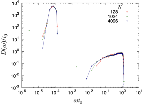
Refer to caption
Figure 15: Double logarithmic plots of Dโ€‹(ฯ‰)๐ท๐œ”D(\omega) against ฯ‰โ€‹t0๐œ”subscript๐‘ก0\omega t_{0} for various N๐‘N at kT/kN=1.0ร—10โˆ’8subscript๐‘˜๐‘‡subscript๐‘˜๐‘1.0superscript108k_{T}/k_{N}=1.0\times 10^{-8}, ฯ•=0.90italic-ฯ•0.90\phi=0.90.

Appendix J Density dependence for DOS

In this Appendix, we investigate the density dependence for the DOS. As shown in Fig. 16 for kT/kN=10โˆ’8subscript๐‘˜๐‘‡subscript๐‘˜๐‘superscript108k_{T}/k_{N}=10^{-8}, the DOS depends on ฯ•italic-ฯ•\phi, where the rotational band shifts to a lower frequency region and the plateau of the translational band becomes longer as the density approaches the jamming point. The latter result is well known from previous studies such as Ref.ย Wyart05 .

Refer to caption
Figure 16: Double logarithmic plots of Dโ€‹(ฯ‰)๐ท๐œ”D(\omega) against ฯ‰โ€‹t0๐œ”subscript๐‘ก0\omega t_{0} for various ฯ•italic-ฯ•\phi at kT/kN=1.0ร—10โˆ’8subscript๐‘˜๐‘‡subscript๐‘˜๐‘1.0superscript108k_{T}/k_{N}=1.0\times 10^{-8} and N=4096๐‘4096N=4096.

References