Formation of Quiescent Prominence Magnetic Field by Supergranulations

Abstract

To understand the formation of quiescent solar prominences, the origin of their magnetic field structures, i.e., magnetic flux ropes (MFRs), must be revealed. We use three-dimensional magnetofriction simulations in a spherical subdomain to investigate the role of typical supergranular motions in the long-term formation of a prominence magnetic field. Time-dependant horizontal supergranular motions with and without the effect of Coriolis force are simulated on the solar surface via Voronoi tessellation. The vortical motions by the Coriolis effect at boundaries of supergranules inject magnetic helicity into the corona. The helicity is transferred and accumulated along the polarity inversion line (PIL) as strongly sheared magnetic field via helicity condensation. The diverging motions of supergranules converge opposite magnetic polarities at the PIL and drive the magnetic reconnection between footpoints of the sheared magnetic arcades to form an MFR. The magnetic network, negative-helicity MFR in the northern hemisphere, and fragmented-to-continuous formation process of magnetic dip regions are in agreement with observations. Although diverging supergranulations, differential rotation, and meridional flows are included, the simulation without the Coriolis effect can not produce an MFR or sheared arcades to host a prominence. Therefore Coriolis force is a key factor for helicity injection and the formation of magnetic structures of quiescent solar prominences.

1 Introduction

Quiescent prominences and filaments are long thin structures of dense and cool plasma that remain stable in the solar corona for days or weeks along the polarity inversion lines (PILs) of quiescent regions (Parenti, 2014). Their magnetic fields have special structures, so-called filament channels, which support the dense mass against gravity (Mackay et al., 2010). The aligned chromospheric fibrils at two sides of a filament (Foukal, 1971) and dominant magnetic field components along the PILs of prominences (Leroy et al., 1983) indicate that filament channels have strongly sheared magnetic fields. The overall magnetic topology of quiescent filament channels is most likely a helical magnetic flux rope (MFR) (Xia et al., 2014b, a; Xia & Keppens, 2016) with plenty of observational evidence, such as the elliptical shape of coronal cavities around quiescent prominences (Gibson et al., 2010), concentric rings of Doppler velocity in coronal cavities (Bak-SteAlicka et al., 2013), persistent swhirling motions of coronal plasma around the center of coronal cavities above prominences (Wang & Stenborg, 2010), and the inverse polarity of prominence magnetic field whose component perpendicular to the PIL is opposite to the one of a potential field (Bommier et al., 1994). Dipped sheared arcades with concave-up magnetic fields (DeVore & Antiochos, 2000) may be the magnetic structure of short filament channels around active regions, but not long ones in quiescent regions (Patsourakos et al., 2020).

Two mechanisms were proposed to explain the formation of MFRs in the corona. The first mechanism suggests that the emergence of the upper part of an MFR from the conversion zone into the corona leads to sheared magnetic arcades (SMAs), arcade-like magnetic loops without concave-up magnetic fields, which are then transformed into an MFR through magnetic reconnection (Fan, 2001). However, this flux emergence mechanism does not apply to the filaments in quiescent regions where no large-scale magnetic flux emergence was found (Mackay et al., 2008). Statistical study of filament observations reveals that over 90% of filaments lie above PILs external to conjugate bipolar fields by flux emergence (Mackay et al., 2008). The second mechanism relies on the shearing, converging, and cancellation of opposite-polarity magnetic flux on the photosphere, which transforms SMAs into a helical MFR by magnetic reconnection in the lower solar atmosphere (Van Ballegooijen & Martens, 1989). This flux cancellation mechanism has been supported by many numerical simulations from magnetofriction models (Mackay & Van Ballegooijen, 2006) and zero-beta magnetohydrodynamic (MHD) models (Amari et al., 1999) to isothermal MHD models (Xia et al., 2014b). However, these models were confronted with three difficulties. First, these models use smooth magnetic flux distributions, which contradicts the observational fact that the photospheric magnetic flux under quiescent filaments is discrete and concentrated as small elements at supergranular boundaries (Zhou et al., 2021). Second, the models relied on large-scale systematic converging flows or equivalent magnetic flux diffusion towards the PIL on the photosphere to drive the flux cancellation. But observations have not found such large-scale flows, instead, supergranular-scale converging flows between diverging supergranules were found both inside and outside filament channels (Rondi et al., 2007; Schmieder et al., 2014). Third, the models required large-scale shearing motions, such as differential rotation, to get shear arcades. However, the differential rotation injects helicity of the opposite sign at west-east oriented PILs in contrast to the observed hemispheric preference (van Ballegooijen et al., 1998), which manifests that filaments with negative (positive) helicity dominate in the northern (southern) hemisphere (Ouyang et al., 2017).

Antiochos (2013) proposed the helicity condensation theory to explain the formation of filament channels. In the theory, photospheric vortical motions between the convective cells inject magnetic helicity into magnetic flux tubes and coronal magnetic reconnections between neighboring flux tubes transfer the injected twist towards the outer periphery of the flux tubes, leading to an inverse cascade of magnetic helicity from small scales to the largest scale at the periphery of the whole magnetic flux system along the PIL, where the helicity condenses and SMAs appear. The theory was demonstrated by ideal MHD simulations based on topological coronal models between two parallel plates (Zhao et al., 2015; Knizhnik et al., 2015) and a Cartesian coronal model with a circular PIL (Knizhnik et al., 2017). These numerical models ignored the primary diverging flows of supergranular cells and simplified the observed cyclonic vortices between the anticyclonic flows of supergranules (Duvall & Gizon, 2000; Langfellner et al., 2015) caused by the Coriolis force (Hathaway, 1982; Egorov et al., 2004), as many annular vortical flows to inject magnetic helicity into corona and produced the SMAs along PILs. Using a large-scale averaged representation of the small-scale vortical motions in magnetofriction simulations, Mackay et al. (2014) found that the helicity condensation can overcome the incorrect sign of helicity injection from differential rotation on a west-east oriented PIL and help to form MFRs in filament channels. In this Letter, we investigate the role of supergranular flows in the formation of the magnetic field of quiescent prominences via magnetofriction simulations.

2 Numerical Methods

The simulation domain is a spherical subdomain extending over radii $r\in[1R_{\odot},1.5R_{\odot}]$, colatitudes $\theta\in[39.6^{\circ},90^{\circ}]$, and longitudes $\phi\in[0^{\circ},60^{\circ}]$ with a 4-level adaptive mesh refinement (AMR) to get $256^{3}$ effective resolution. From a smooth bipolar photospheric magnetogram, we use the spherical potential field extrapolation module in the PDFI_SS software (Fisher et al., 2020) to extrapolate the initial potential magnetic field. We solve the magnetofriction equations (Guo et al., 2016) without explicit resistivity using the code MPI-AMRVAC (Porth et al., 2014; Xia et al., 2018). Magnetic reconnection here is caused by numerical resistivity. The magnetofrictional velocity $v=\mathbf{J}\times\mathbf{B}/(\nu_{0}B^{2})$, where $\nu_{0}=10^{-15}$ s cm^-2 is the viscous coefficient, has a smooth decay to zero towards the photosphere (Cheung & DeRosa, 2012) and an upper limit of $30$ km s^-1 (Pomoell et al., 2019). We use the constrained transport (CT) scheme (Gardiner & Stone, 2005), with the HLL flux for the electric field, on the staggered AMR mesh (Olivares et al., 2019) to keep magnetic field divergence-free. Boundary conditions are periodic on the longitudinal boundaries, open on the outer radial boundary, and closed on the latitudinal boundaries. On the photospheric boundary, we use zero normal velocity with the supergranular horizontal velocity field described as follows.

A Voronoi tessellation of solar surface resembles (super)granular segmentation in both topology and statistics (Schrijver et al., 1997). We use a weight function $\omega=3|\sin(\pi t/\tau+\xi)|+0.7$ to generate Voronoi tessellation, in which $\tau$ is the lifetime of a supergranular cell with a Gaussian random distribution centered on 1.6 days (Hirzberger et al., 2008) and $\xi$ is the random initial phase. We use 1 as the lower limit of the weights for living cells, smaller weights are set to zero to remove the corresponding cells from the tessellation map. So the simulated supergranular cells are changing with time with their area proportional to their weights. We adopt the dimensionless diverging velocity within supergranular cells as $v_{r}(r)=2r^{2}/r_{0}\exp(-4r^{2}/r_{0}^{2})$ (Gudiksen & Nordlund, 2005), where $r$ is the spherical distance to the cell center and $r_{0}$ is the radius of a circle with area equal to the supergranular cell. The vortical velocity due to Coriolis force acting on the diverging horizontal flows is simplified as $v_{t}(r)=2r/r_{0}v_{r}(r)$ neglecting the latitude-dependence of Coriolis force. We use a normalization factor to make sure the maximal supergranular speed is initially 500 m s^-1. The velocities of differential rotation and meridional flow (Mackay et al., 2014) are also included. We multiply the total driving speed by 5 to speed up the long-term evolution. Dimensionless values in our results have the time unit of 8.3 hours and the magnetic field unit of 2 Gauss. We have run a model SR with supergranules rotating under Coriolis force and a model SS without the Coriolis effect.

3 Results

Initially (Figure 1 (a)), the magnetic field is a bipolar arcade rooted in the smooth positive (red) and negative (blue) polarity regions separated by a straight north-south directed PIL. Then, the supergranular diverging flows transport and concentrate magnetic flux to the boundaries of supergranules forming a magnetic network, and the differential rotation gradually shifts the northern part of magnetic flux to the east and the southern part to the west making the PIL tilted anticlockwise. At time 30 (Figure 1 (b)), short magnetic loops near the PIL have skewed away from the initial potential field state. The skew angle, defined as the angle between the horizontal component of the magnetic field above the PIL and the horizontal direction perpendicular to the PIL (Mackay & van Ballegooijen, 2001), is about 45 degrees. Long loops, which root in the central region of each polarity far from the PIL, remain in an approximately potential state with neglilible skew angles during the whole evolution. At time 60 (Figure 1 (c)), low-lying magnetic loops near the PIL are almost aligned with the PIL with large skew angles and some of them are changed into helical field lines (red line) along the PIL. At time 90 (Figure 1 (d)), more helical field lines form and enwind the earlier-born helical lines assembling a low-lying thin MFR along the PIL. Later at time 120 (Figure 1 (e)), which is after 41.5 days, the MFR matures with a larger height and cross-section size suitable for hosting a quiescent prominence. Different from earlier MFR models in which helical field lines root in two compact regions, the footpoints of this MFR distribute extensively along the PIL. In contrast to model SR, model SS does not produce any MFR or SMAs until time 120 (Figure 1 (f)), and all magnetic loops stay nearly potential for another 120 time.

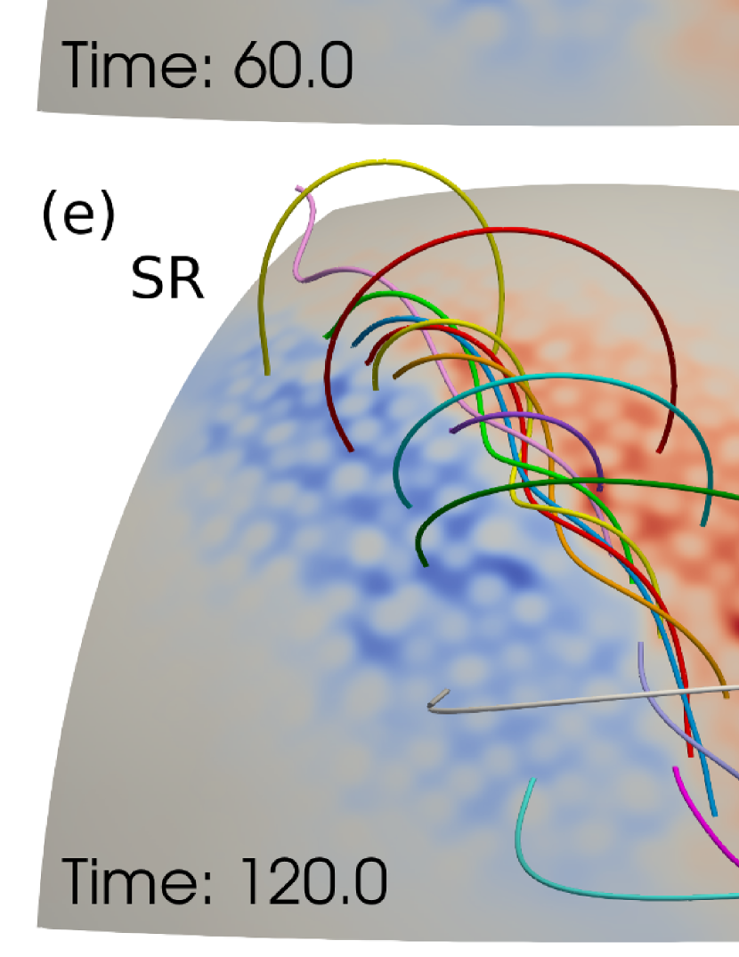
Figure 1: Magnetic field lines of model SR with Coriolis effect at time 0 (a), 30 (b), 60 (c), 90 (d), and 120 (e) in contrast to model SS without Coriolis effect at time 120 (f). The photosphere is colored by the radial magnetic field in red-to-blue colors saturated at $\pm$18 G.

To understand the origin of the sheared magnetic loops, we illustrate the build-up process of the sheared loops of model SR in the left column of Figure 2. For comparison, a similar representation of model SS at the same time is plotted in the right column. In panels (a)-(f), the magnetic loops crossing over the cyan PIL at different heights are plotted in rainbow colors. At time 15, the lowest blue loop in model SR has a short length and a small skew angle to the PIL, while the loops in model SS have nearly zero skew angles. For model SR at later times 45 and 60, several loops close to the PIL are sheared and the lowest loop has the fastest growth rate in the skew angle and length. Further away from the PIL, loops with higher altitudes have smaller skew angles. In contrast, loops in model SS at all heights and distances from the PIL, remain roughly perpendicular to the PIL. The sheared loops with large skew angles in model SR are not created by persistent photospheric shearing flows, because such shearing flows along the PIL do not exist. Instead, only vortical diverging and converging flows by supergranules exist as shown by grey arrows in panels (g) and (h). A logical explanation of the strongly sheared loops around the PIL in model SR is referable to the helicity condensation theory (Antiochos, 2013). Vortical converging flows towards the junctions of several supergranules inject negative magnetic helicity into the magnetic flux tubes with footpoints at strong magnetic flux on the photosphere. Component magnetic reconnection happens on the interface of adjacent twisted flux tubes, which transports the twisted flux to the common periphery of the flux tubes and leaves behind the untwisted flux in the central regions. This process inversely cascades from small scales to large scales until reaching the biggest flux tube representing the whole bipolar region with part of the periphery folded around the PIL, where twisted fluxes with negative helicity condense as SMAs.

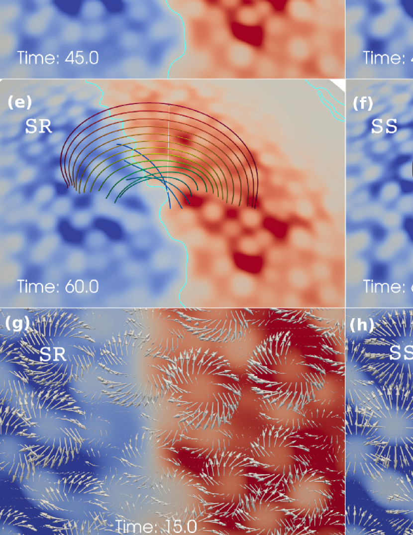
Figure 2: Comparative views of model SR and SS at time 15, 45, and 60. In panel (a)-(f), magnetic field lines, in rainbow colors, are integrated from uniformly sampled seed points along a radial white line starting from the cyan PIL at a fixed latitude. The photosphere is colored by radial magnetic field saturated at $\pm$20 G. Zoom-in views at time 15 are shown in panel (g) and (h), where grey arrows present the photospheric horizontal velocity field.

Then we present how much the magnetic helicity is injected into the corona and how the magnetic free energy is stored in our models. The flux of (relative) magnetic helicity through the photosphere is defined by the equation with zero resistivity (Berger & Field, 1984):

$$\frac{dH_{R}}{dt}=-2\int\mathbf{A}^{P}\times\mathbf{E}\cdot d\mathbf{S}=-2\int(A^{P}_{\theta}E_{\phi}-A^{P}_{\phi}E_{\theta})dS$$ (1)

where $\mathbf{A}^{P}$ is the vector potential of the potential magnetic field which matches the instantaneous photospheric $B_{r}$, $\mathbf{E}$ is the electric field and quantified as the electric field from the CT scheme, and $d\mathbf{S}$ is the surface element with normal direction $\mathbf{\hat{r}}$. Figure 3 (a) shows the time evolution of the magnetic helicity fluxes through the photosphere in model SR as the total (solid line), the negative (dashed line), and the positive flux (dotted line). The positive helicity flux is about 20 to 30 times larger than the negative helicity flux. Magnetic helicity fluxes through other boundaries are negligible. The photospheric distribution of the integrand in equation (1) is shown in Figure 3 (d) with horizontal velocity vectors and contours of $B_{r}$ overplotted. The positive values of the integrand are distributed in the outer regions of supergranules in donut shapes, induced by the clockwise rotating diverging flows of supergranules. The negative values are distributed sporadically along the borders of several supergranules and caused by irregular counterclockwise converging flows towards strong magnetic flux. For model SS as shown in panel (b), the positive and negative helicity flux almost cancel out with a small positive total flux. Panel (e) for model SS shows that positive values alternates with negative values in the outer region of supergranules. Figure 3 (c) presents the time evolution of the magnetic free energy, which is obtained by subtracting the potential field energy from the total magnetic energy. Both models have an increasing magnetic free energy, while the magnetic free energy in model SR increases about three times faster than it in model SS.

Figure 3: (a) Time evolution of the magnetic helicity fluxes as the total (solid line), the negative (dashed line), and the positive (dotted line) ones through the photosphere of model SR. (b) Similar curves as (a) for model SS. (c) Time evolution of the magnetic free energy of model SR (solid line) and SS (dashed line). (d) Magnetic helicity flux density on the photosphere overlaid with horizontal velocity field as yellow arrows and contours of $B_{r}$ at $\pm 16$ G for model SR at time 36. (e) Similar plot as (d) for model SS.

Long-lived prominence plasma should be supported by magnetic tension force against downward gravity in locally concave-up magnetic fields, i.e., magnetic dips. We locate the magnetic dip regions (MDRs) where the radial component of the curvature of magnetic field lines is positive and the radial component of the magnetic field has less than 10% proportion. Figure 4 presents snapshots of the formation of magnetic dips from the top views in upper panels (a)-(b) and from the side views in lower pannels (a1)-(b1). At time 61.2, small isolated MDRs distribute along the PIL with supergranular scale intervals. Later at time 82.8, the small MDRs grow horizontally along the PIL and connect to form three long MDRs. Helical field lines tangential to the photosphere outline the periphery of an MFR above the PIL and the MDRs naturally appear in the lower half of the MFR. At time 120, further growth and connection of MDRs result in a long slab-like MDR with a growing height reaching 28,000 km and a length of about 480,000 km. The MFR surrounding the MDR has helical field lines winding 1 to 2 turns around a common axis. If the MDRs are filled with prominence plasma, the formation process of MDRs is consistent with filament observations showing that quiescent filaments form from aligned fragments to a continuous body (Pevtsov & Neidig, 2005).

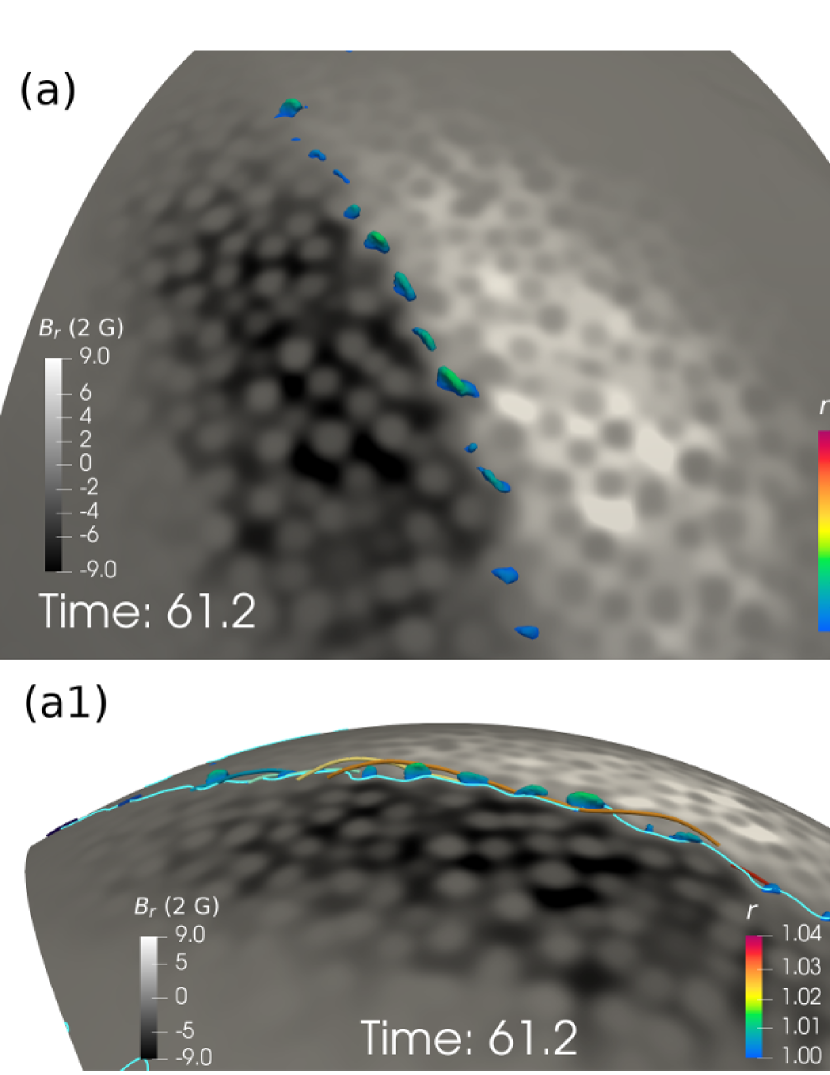
Figure 4: Formation of magnetic dip regions shown as isosurfaces colored by solar radius $r$ from top views (a)-(c) and from side views (a1)-(c1) at time 61.2, 82.8, and 120. Surrounding magnetic field lines in different colors and the main PIL in cyan are plotted in (a1)-(c1) additionally.

To understand the transition from SMAs to MFRs, we find the sites of magnetic reconnection and flux cancellation on the photosphere. In Figure 5 (a), the footpoints of the pink and the sky blue field line, in the middle of the panel, converge to the white PIL by adjacent supergranular flows indicated by the purple arrows, and the two field lines are about to be reconnected at the PIL to form a helical field line like the yellow one. Similarly, the blue and the red field line will be reconnected to form a helical field line like the green one in the lower right region. Figure 5 (b) presents a zoom-out side view of these field lines above the photospheric supergranular cells. The sites of magnetic reconnection are at the borders of supergranular cells on two sides of the PIL. Some parts of the PIL crossing through supergranular cells are bald patches where the MFR touches the photosphere. Evidence of magnetic flux cancellation is shown in Figure 5 (c) in which the time evolution of the total unsigned magnetic flux on the photosphere is plotted for both models. After a short period of flux dispersion without many cancellations, the unsigned magnetic flux of model SR decreases linearly losing about 20 % until time 120, which indicates continuous flux cancellation. The unsigned magnetic flux of model SS decreases less than 3 % until time 70 and then slightly increases with small oscillation and slow flux cancellation. The slight increase is caused by numerical error of the magnetic boundary condition.

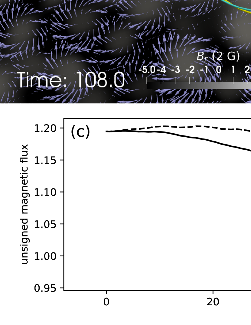
Figure 5: Linking sheared loops to helical field lines via photospheric magnetic reconnection along the white PIL. (a) Top view of 6 selected magnetic field lines above the photospheric magnetogram with arrows presenting horizontal velocity. (b) Side view of the same magnetic field lines in (a) above a photospheric color map presenting supergranular cells. (c) Evolution of total unsigned magnetic flux on photosphere for SR (solid line) and SS (dashed line) model.

4 Discussion and Conclusions

The only difference in model setup between model SR and SS is the vortical motions by Coriolis force, which leads to strikingly different results, namely, an MFR in model SR and potential arcades in model SS. The counterclockwise vortical flows in strong magnetic flux regions around supergranular boundaries inject negative magnetic helicity, which is accumulated along the PIL via helicity condensation to form a dextral filament channel in the northern hemisphere. Therefore Coriolis force is a key factor for helicity injection and formation of quiescent prominences, while effective magnetic flux diffusion by supergranular flows (Leighton, 1964) and differential rotation are not the main reasons for the formation of filament channels. We will include the latitude dependence of the Coriolis effect (Duvall & Gizon, 2000) in the future expecting faster MFR formation at higher latitudes.

The helicity condensation theory descibes how the injected magnetic helicity at small scale is transferred and condensed to the PIL, which explain the origin of strong axial magnetic flux along quiescent filament channels. But this theory can only lead to SMAs, which contradict the observational evidence (Bak-SteAlicka et al., 2013; Wang & Stenborg, 2010) of quiescent prominences. Previous numerical simulations on helicity condensation (Zhao et al., 2015; Knizhnik et al., 2015, 2017) did not produce MFRs because of the absent of the primary diverging motions of supergranules, which not only generate the magnetic network but also converge opposite magnetic polarities at the PIL and drive the magnetic reconnection between footpoints of SMAs, the magnetic flux cancellation in forming filament channels (Wang & Muglach, 2007), and the formation of MFRs.

During the formation of the coherent MFR in model SR, a chain of small MFRs first forms along the PIL with fragmented small MDRs to host prominence plasma. Later on, these small MFRs and MDRs grow and merge with neighbors to form the mature MFR, which is consistent with the “head-to-tail” conceptual model of prominence formation proposed by Martens & Zwaan (2001). The isolated MDRs consist of piled-up magnetic dips from the photosphere may correspond to the observed pillars or legs of quiescent prominences (Li & Zhang, 2013; Zhou et al., 2021). We run models starting from west-to-east PILs to simulate high-latitude quiescent prominences and formed MFRs to be reported in a follow-up paper.

References

- Amari et al. (1999) Amari, T., Luciani, J. F., Mikic, Z., & Linker, J. 1999, The Astrophysical Journal Letters, 518, L57
- Antiochos (2013) Antiochos, S. K. 2013, The Astrophysical Journal, 772, 72, doi: 10.1088/0004-637X/772/1/72
- Bak-SteAlicka et al. (2013) Bak-SteAlicka, U., Gibson, S. E., Fan, Y., et al. 2013, The Astrophysical Journal, 770, L28, doi: 10.1088/2041-8205/770/2/L28
- Berger & Field (1984) Berger, M. A., & Field, G. B. 1984, Journal of Fluid Mechanics, 147, 133, doi: 10.1017/S0022112084002019
- Bommier et al. (1994) Bommier, V., Degl’Innocenti, E. L., Leroy, J. L., & Sahal-Brechot, S. 1994, Solar Physics, 154, 231
- Cheung & DeRosa (2012) Cheung, M. C. M., & DeRosa, M. L. 2012, The Astrophysical Journal, 757, 147, doi: 10.1088/0004-637X/757/2/147
- DeVore & Antiochos (2000) DeVore, C. R., & Antiochos, S. K. 2000, The Astrophysical Journal, 539, 954
- Duvall & Gizon (2000) Duvall, T. L., & Gizon, L. 2000, Solar Physics, 192, 177, doi: 10.1007/978-94-011-4377-6_10
- Egorov et al. (2004) Egorov, P., Rudiger, G., & Ziegler, U. 2004, Astronomy and Astrophysics, 425, 725, doi: 10.1051/0004-6361:20040531
- Fan (2001) Fan, Y. 2001, The Astrophysical Journal Letters, 554, L111
- Fisher et al. (2020) Fisher, G. H., Kazachenko, M. D., Welsch, B. T., et al. 2020, The Astrophysical Journal Supplement Series, 248, 2, doi: 10.3847/1538-4365/ab8303
- Foukal (1971) Foukal, P. 1971, Solar Physics, 19, 59
- Gardiner & Stone (2005) Gardiner, T. A., & Stone, J. M. 2005, Journal of Computational Physics, 205, 509, doi: 10.1016/j.jcp.2004.11.016
- Gibson et al. (2010) Gibson, S. E., Kucera, T. A., Rastawicki, D., et al. 2010, The Astrophysical Journal, 724, 1133, doi: 10.1088/0004-637X/724/2/1133
- Gudiksen & Nordlund (2005) Gudiksen, B. V., & Nordlund, A. 2005, The Astrophysical Journal, 618, 1020
- Guo et al. (2016) Guo, Y., Xia, C., Keppens, R., & Valori, G. 2016, The Astrophysical Journal, 828, 82, doi: 10.3847/0004-637X/828/2/82
- Hathaway (1982) Hathaway, D. H. 1982, Solar Physics, 77, 341. http://articles.adsabs.harvard.edu/pdf/1982SoPh...77..341H
- Hirzberger et al. (2008) Hirzberger, J., Gizon, L., Solanki, S. K., & Duvall, T. L. 2008, Solar Physics, 251, 417, doi: 10.1007/s11207-008-9206-8
- Knizhnik et al. (2015) Knizhnik, K. J., Antiochos, S. K., & DeVore, C. R. 2015, The Astrophysical Journal, 809, 137, doi: 10.1088/0004-637X/809/2/137
- Knizhnik et al. (2017) Knizhnik, K. J., Antiochos, S. K., DeVore, C. R., & Wyper, P. F. 2017, The Astrophysical Journal, 851, L17, doi: 10.3847/2041-8213/aa9e0a
- Langfellner et al. (2015) Langfellner, J., Gizon, L., & Birch, A. C. 2015, Astronomy & Astrophysics, 581, A67, doi: 10.1051/0004-6361/201526024
- Leighton (1964) Leighton, R. B. 1964, The Astrophysical Journal, 140, 1547, doi: 10.1086/148058
- Leroy et al. (1983) Leroy, J. L., Bommier, V., & Sahal-Brechot, S. 1983, Solar Physics, 83, 135
- Li & Zhang (2013) Li, L., & Zhang, J. 2013, Solar Physics, 282, 147, doi: 10.1007/s11207-012-0122-6
- Mackay et al. (2014) Mackay, D. H., DeVore, C. R., & Antiochos, S. K. 2014, The Astrophysical Journal, 784, 164, doi: 10.1088/0004-637X/784/2/164
- Mackay et al. (2008) Mackay, D. H., Gaizauskas, V., & Yeates, A. R. 2008, Solar Physics, 248, 51, doi: 10.1007/s11207-008-9127-6
- Mackay et al. (2010) Mackay, D. H., Karpen, J. T., Ballester, J. L., Schmieder, B., & Aulanier, G. 2010, Space Sci. Rev., 151, 333, doi: 10.1007/s11214-010-9628-0
- Mackay & van Ballegooijen (2001) Mackay, D. H., & van Ballegooijen, A. A. 2001, The Astrophysical Journal, 560, 445, doi: 10.1086/322385
- Mackay & Van Ballegooijen (2006) Mackay, D. H., & Van Ballegooijen, A. A. 2006, The Astrophysical Journal, 641, 577
- Martens & Zwaan (2001) Martens, P. C., & Zwaan, C. 2001, The Astrophysical Journal, 558, 872
- Olivares et al. (2019) Olivares, H., Porth, O., Davelaar, J., et al. 2019, Astronomy & Astrophysics, 629, A61, doi: 10.1051/0004-6361/201935559
- Ouyang et al. (2017) Ouyang, Y., Zhou, Y. H., Chen, P. F., & Fang, C. 2017, The Astrophysical Journal, 835, 94, doi: 10.3847/1538-4357/835/1/94
- Parenti (2014) Parenti, S. 2014, Living Reviews in Solar Physics, 11, doi: 10.12942/lrsp-2014-1
- Patsourakos et al. (2020) Patsourakos, S., Vourlidas, A., Torok, T., et al. 2020, Space Science Reviews, 216, 131, doi: 10.1007/s11214-020-00757-9
- Pevtsov & Neidig (2005) Pevtsov, A. A., & Neidig, D. 2005, in ASP Conference Series, Vol. 346, 219–226. http://adsabs.harvard.edu/abs/2005ASPC..346..219P
- Pomoell et al. (2019) Pomoell, J., Lumme, E., & Kilpua, E. 2019, Solar Physics, 294, 41, doi: 10.1007/s11207-019-1430-x
- Porth et al. (2014) Porth, O., Xia, C., Hendrix, T., Moschou, S. P., & Keppens, R. 2014, The Astrophysical Journal Supplement Series, 214, 4, doi: 10.1088/0067-0049/214/1/4
- Rondi et al. (2007) Rondi, S., Roudier, T., Molodij, G., et al. 2007, Astronomy & Astrophysics, 467, 1289, doi: 10.1051/0004-6361:20066649
- Schmieder et al. (2014) Schmieder, B., Roudier, T., Mein, N., et al. 2014, Astronomy & Astrophysics, 564, A104, doi: 10.1051/0004-6361/201322861
- Schrijver et al. (1997) Schrijver, C. J., Hagenaar, H. J., & Title, A. M. 1997, The Astrophysical Journal, 475, 328
- van Ballegooijen et al. (1998) van Ballegooijen, A. A., Cartledge, N. P., & Priest, E. R. 1998, The Astrophysical Journal, 501, 866, doi: 10.1086/305823
- Van Ballegooijen & Martens (1989) Van Ballegooijen, A. A., & Martens, P. C. H. 1989, The Astrophysical Journal, 343, 971
- Wang & Muglach (2007) Wang, Y.-M., & Muglach, K. 2007, The Astrophysical Journal, 666, 1284
- Wang & Stenborg (2010) Wang, Y.-M., & Stenborg, G. 2010, The Astrophysical Journal, 719, L181, doi: 10.1088/2041-8205/719/2/L181
- Xia & Keppens (2016) Xia, C., & Keppens, R. 2016, The Astrophysical Journal, 823, 22, doi: 10.3847/0004-637X/823/1/22
- Xia et al. (2014a) Xia, C., Keppens, R., Antolin, P., & Porth, O. 2014a, The Astrophysical Journal, 792, L38, doi: 10.1088/2041-8205/792/2/L38
- Xia et al. (2014b) Xia, C., Keppens, R., & Guo, Y. 2014b, The Astrophysical Journal, 780, 130, doi: 10.1088/0004-637X/780/2/130
- Xia et al. (2018) Xia, C., Teunissen, J., Mellah, I. E., Chane, E., & Keppens, R. 2018, The Astrophysical Journal Supplement Series, 234, 30, doi: 10.3847/1538-4365/aaa6c8
- Zhao et al. (2015) Zhao, L., DeVore, C. R., Antiochos, S. K., & Zurbuchen, T. H. 2015, The Astrophysical Journal, 805, 61, doi: 10.1088/0004-637X/805/1/61
- Zhou et al. (2021) Zhou, C., Xia, C., & Shen, Y. 2021, Astronomy & Astrophysics, 647, A112, doi: 10.1051/0004-6361/202039558