Benign, Tempered, or Catastrophic:
A Taxonomy of Overfitting

Abstract

The practical success of overparameterized neural networks has motivated the recent scientific study of interpolating methods, which perfectly fit their training data. Certain interpolating methods, including neural networks, can fit noisy training data without catastrophically bad test performance, in defiance of standard intuitions from statistical learning theory. Aiming to explain this, a body of recent work has studied benign overfitting, a phenomenon where some interpolating methods approach Bayes optimality, even in the presence of noise. In this work we argue that while benign overfitting has been instructive and fruitful to study, many real interpolating methods like neural networks do not fit benignly: modest noise in the training set causes nonzero (but non-infinite) excess risk at test time, implying these models are neither benign nor catastrophic but rather fall in an intermediate regime. We call this intermediate regime tempered overfitting, and we initiate its systematic study. We first explore this phenomenon in the context of kernel (ridge) regression (KR) by obtaining conditions on the ridge parameter and kernel eigenspectrum under which KR exhibits each of the three behaviors. We find that kernels with powerlaw spectra, including Laplace kernels and ReLU neural tangent kernels, exhibit tempered overfitting. We then empirically study deep neural networks through the lens of our taxonomy, and find that those trained to interpolation are tempered, while those stopped early are benign. We hope our work leads to a more refined understanding of overfitting in modern learning.

1 Introduction

In the last decade, the dramatic success of overparameterized deep neural networks (DNNs) has inspired the field to reexamine the theoretical foundations of generalization. Classical statistical learning theory suggests that an algorithm which interpolates (i.e. perfectly fits) its training data will typically catastrophically overfit at test time, generalizing no better than a random function

Figure 1c illustrates the catastrophic overfitting classically expected of an interpolating method. Defying this picture, DNNs can interpolate their training data and generalize well nonetheless (Neyshabur et al., 2015; Zhang et al., 2017), suggesting the need for a new theoretical paradigm within which to understand their overfitting.

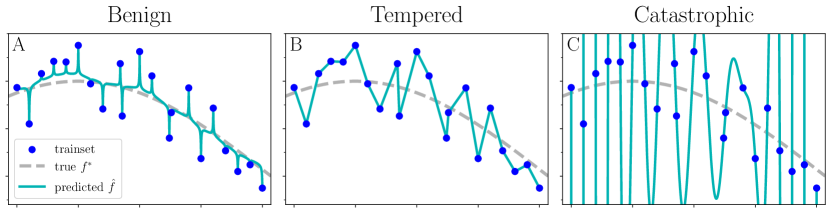
Figure 1: As $n\rightarrow\infty$, interpolating methods can exhibit three types of overfitting. (A) In benign overfitting, the predictor asymptotically approaches the ground-truth, Bayes-optimal function. Nadaraya-Watson kernel smoothing with a singular kernel, shown here, is asymptotically benign. (B) In tempered overfitting, the regime studied in this work, the predictor approaches a constant test risk greater than the Bayes-optimal risk. Piecewise-linear interpolation is asymptotically tempered. (C) In catastrophic overfitting, the predictor generalizes arbitrarily poorly. Rank-$n$ polynomial interpolation is asymptotically catastrophic.

This need motivated the identification and study of benign overfitting using the terminology of (Bartlett et al., 2020) (also called “harmless interpolation” (Muthukumar et al., 2020)), a phenomenon in which certain methods that perfectly fit the training data still approach Bayes-optimal generalization in the limit of large trainset size. Intuitively speaking, benignly-overfitting methods fit the target function globally, yet fit the noise only locally, and the addition of more label noise does not asymptotically degrade generalization. Figure 1a illustrates a simple method that is asymptotically benign. The study of benign overfitting has proven fruitful, leading to rich mathematical insights into high-dimensional learning, and benign overfitting is certainly closer to the real behavior of DNNs than catastrophic overfitting.

That said, it requires only simple experiments to reveal that many standard DNNs do not overfit benignly: when training on noisy data, DNNs do not diverge catastrophically, but neither do they approach Bayes-optimal risk. Instead, they converge to a predictor that is neither catastrophic nor optimal but rather somewhere in between, with error that increases as the noise in the data increases. Figure 2 depicts such an experiment: a ResNet is trained on a binary variant of CIFAR-10 with varying amounts of training label noise, and with increasing sample size $n$. We see from Figure 2 that greater train noise indeed results in greater test error, and this test error persists even as $n$ grows, converging to a non-zero asymptotic value. This is unlike “benign overfitting,” which would produce an asymptotically-optimal predictor at all non-trivial noise levels (depicted in blue in Figure 2). This suggests that, in the search for a paradigm to understand modern interpolating methods, we should identify and study a regime intermediate between benign and catastrophic.

1.1 Summary of Contributions

In this work we formally identify an intermediate regime between benign and catastrophic overfitting. We call this intermediate behavior tempered overfitting because the noise’s harmful effect is tempered but still nonzero. We find that both DNNs trained to interpolation and (ridgeless) kernel regression (KR) using certain common kernels fall into this intermediate regime even as the number of training examples $n$ approaches infinity, as do common methods like 1-nearest-neighbors and piecewise-linear interpolation (as in Figure 1b). Our tempered regime completes the taxonomy of overfitting: essentially any learning procedure is either benign, tempered, or catastrophic in the asymptotic limit.

We begin in Section 2 with preliminaries, formal definitions of the three regimes, and a taxonomy of some common ML methods according to these regimes. We generally consider an algorithm’s limiting behavior as $n\rightarrow\infty$, as in the study of statistical consistency. We are more interested in algorithms’ asymptotic test risk than in the fact that they interpolate, and we consider certain non-interpolating methods as well as interpolating methods. In Section 3, we study these three regimes for kernel regression (KR). Using recent spectral theories characterizing the expected test error of KR, we obtain conditions on the ridge parameter and kernel eigenspectrum under which KR falls into each of the three regimes. Importantly, we find that ridgeless kernels with powerlaw spectra, including the Laplace kernel and ReLU fully-connected neural tangent kernels (NTKs), are asymptotically tempered, not benign. We confirm our theory with experiments on synthetic data. In Section 4, we empirically study overfitting for DNNs. We give evidence that standard DNNs trained to interpolation exhibit tempered overfitting, not benign overfitting, motivating the further study of tempered overfitting in the pursuit of understanding modern machine learning methods. We additionally study the time dynamics of overfitting, and the effect of early-stopping. We conclude with discussion in Sections 5 and 6.

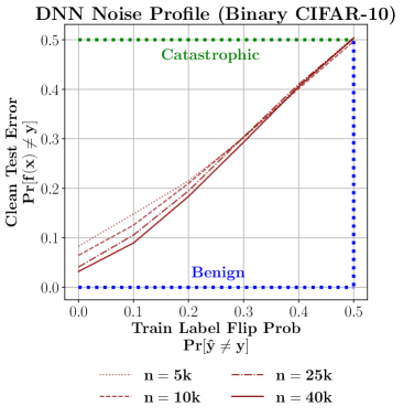
Figure 2: DNNs trained on image data exhibit tempered overfitting, not benign overfitting. Curves show test classification error vs. training label flip probability for a Wide ResNet $28\times 10$ trained to interpolation on binary CIFAR-10 (animals vs. vehicles) for different training sizes $n$. These curves are noise profiles, as discussed in Section 2.

1.2 Relation to Prior Work

Our work is inspired by recent developments in the theory and empirics of interpolating methods (Belkin et al., 2019d, c, 2018a; Bartlett et al., 2020; Rakhlin and Zhai, 2019; Ji et al., 2021; Devroye et al., 1998; Koehler et al., 2021; Liang and Rakhlin, 2018, 2020; Muthukumar et al., 2020; Tsigler and Bartlett, 2020). Many of these works prove that certain interpolating estimators are statistically consistent in certain settings, demonstrating benign overfitting. In contrast, we argue that a wide range of interpolators, including DNNs used in practice, are not benign. Our work is compatible with prior work because we consider different settings—erring more on the side of realism—which leads us to different conclusions. The empirical observation that interpolating DNNs for classification are inconsistent, and thus not benign, was made in Nakkiran and Bansal (2020), which in part inspired the present work.

Briefly, many prior works assume that the target task always lies in “high enough dimension” relative to the number of samples $n$, while our work considers the limit $n\to\infty$ for tasks of fixed dimension $d$, the realistic asymptotic in practice. For example, in the linear regression setting, Bartlett et al. (2020) highlight that benign overfitting occurs most robustly when input dimension grows faster than the sample size. Other works explicitly scale the ambient problem dimension and sample size to infinity together at a proportional rate (Hastie et al., 2019; Mei and Montanari, 2019; Liang and Rakhlin, 2018). This joint scaling is also often considered in statistical physics approaches to learning dynamics (see Zdeborová and Krzakala (2016) and references therein). Taking a different approach, Frei et al. (2022) prove that interpolating two-layer networks can achieve close to optimal test error on certain distributions, but require an assumption that $n\leq\Omega(d)$. And Koehler et al. (2021) state a generalization bound for interpolators that decays to $0$ with $n$, but also requires $n\leq d$. In summary, a bulk of prior benign overfitting results apply in the regime where $n$ is large, but still restricted to be smaller than the dimension of the problem, whereas we do not consider such restrictions.

Our work is also compatible with prior works which observe that excess risk of certain interpolating methods decays with ambient dimension, interpreted as high-dimensional problems enjoying a “blessing of dimensionality.” For example, the simplicial interpolation scheme of Belkin et al. (2018a) has excess risk that decays as $O(2^{-d})$ for ambient dimension $d$, and Rakhlin and Zhai (2019) show that kernel ridgeless regression with the Laplace kernel is inconsistent in any fixed dimension, but with a lower bound on risk that decays with dimension. We find an explicit result to this effect when studying KR: for Laplace kernels and ReLU NTKs, asymptotic excess mean squared error decays like $\Theta(1/d)$. These phenomena support our claim that many interpolating methods are tempered on real distributions, which have fixed dimension.

Though most results of Bartlett et al. (2020) treat linear regression with dimension that grows with $n$, their Theorem 6 shows that benign overfitting can occur in a static infinite-dimensional setting if the eigenvalues of the covariance matrix decay at a particular slow rate, with faster decay than this giving non-benign behavior. Our Theorem 3.1, which is our main theoretical result, essentially subsumes this: we recover this fragile condition for benign overfitting and also derive spectral conditions under which faster decays give either tempered or catastrophic overfitting.

Our KR setting is similar but slightly different from that of Bartlett et al. (2020) and merits a brief discussion. Bartlett et al. (2020) study infinite-dimensional linear regression with sub-Gaussian features and a fixed covariance spectrum, and proceed to obtain upper and lower bounds on test risk that permit one to determine whether fitting is benign. This setting is mathematically equivalent to KR with random sub-Gaussian eigenfunctions. Our setting is essentially KR with random Gaussian eigenfunctions. Instead of studying KR generalization from scratch, we simply use recent results using methods from statistical mechanics to derive fairly explicit closed-form expressions for the expected test MSE of KR with Gaussian features in terms of the kernel spectrum (Bordelon et al., 2020; Canatar et al., 2021; Jacot et al., 2020; Simon et al., 2021). The result which we use as our starting point is rather simple, and our proofs are consequently quite straightforward and extensible.

Our Theorem 3.1 includes the surprisingly simple result that, for KR with a kernel with a powerlaw eigenspectrum with exponent $\alpha$, the kernel overfits target noise by a factor of $(\alpha-1)$ as $n\rightarrow\infty$, implying that the method is tempered. The fact that this overfitting factor is $\Theta(1)$ can be obtained by assembling several results of Jacot et al. (2020), though their analysis does not provide the value of the constant. The asymptotic behavior of powerlaw KR was also studied by Spigler et al. (2020), though they assume zero noise, while noise is central to the present work. Cui et al. (2021) also study the asymptotics of powerlaw KR and find as we do that, when the ridge parameter is negligible, test risk plateaus as $n\rightarrow\infty$, though they also do not find the value of the asymptotic risk.

2 The Three Types of Overfitting

Here we formally present our taxonomy of overfitting, delineating the three types of asymptotic behaviors which learning procedures can exhibit.

2.1 Definitions

We consider a fairly generic in-distribution supervised learning setting. For simplicity, we present definitions for regression, but these are readily extended to classification. We wish to learn a function $\widehat{f}:\mathcal{X}\to\mathbb{R}$ from a size-$n$ dataset of i.i.d. samples $\mathcal{D}_{n}\equiv\{(x_{i},y_{i})\}_{i=1}^{n}\sim\mathcal{D}$, where $\mathcal{D}$ is a joint distribution over $\mathcal{X}\times\mathbb{R}$, and $\mathcal{X}$ is the input domain. We shall generally assume nonzero target noise, with $\text{Var}[y_{i}|x_{i}]>0$. We evaluate the generalization performance of $\widehat{f}$ by the mean squared error (MSE): $R(\widehat{f}):=\mathop{\mathbb{E}}_{x,y\sim\mathcal{D}}\left[(\widehat{f}(x)-y)^{2}\right]$. The Bayes-optimal regression function is given by $f^{*}:=\operatorname*{argmin}_{f}R(f)$, where the minimization is over all measurable functions, and has risk $R^{*}$ which is called the irreducible risk. The excess risk of any function $\widehat{f}$ is given by $\overline{R}(\widehat{f}):=R(\widehat{f})-R^{*}$. We say an estimator achieves interpolation if $\widehat{f}_{n}(x_{i})=y_{i}$ for all $(x_{i},y_{i})\in\mathcal{D}_{n}$. These definitions are readily generalized to classification, using classification error in place of MSE.

Learning Procedure.

The objects of study in our taxonomy are learning procedures. Our definition of a learning procedure is quite general, allowing discussion of methods from DNNs to 1-nearest-neighbors. Informally, a learning procedure is simply a specification of which model to output on a given train set of a given size.

Formally, a learning procedure $\mathcal{A}:=\{A_{n}\}_{n}$ is a sequence of (potentially stochastic) functions, indexed by sample size $n\in\mathbb{N}$. At each $n$, the function $A_{n}:\mathcal{D}_{n}\mapsto\widehat{f}_{n}$ inputs a train set $\mathcal{D}_{n}$ and outputs a “model” $\widehat{f}_{n}:\mathcal{X}\to\mathbb{R}$. Note that this $n$-dependence allows learning procedures to be non-uniform, varying the learning algorithm with sample size $n$. For example, it allows procedures which scale up a DNN or narrow a kernel bandwidth as $n$ grows. The expected risk of a learning procedure on $n$ examples from distribution $\mathcal{D}$ is $\mathcal{R}_{n}:=\mathop{\mathbb{E}}_{A_{n},\mathcal{D}_{n}}[R(A_{n}(\mathcal{D}_{n}))]$.

2.2 The Taxonomy

We shall categorize learning procedures in terms of their asymptotic expected risk. We handle regression and $K$-class classification settings separately, due to their different loss scalings. As the number of samples $n\to\infty$, the sequence of expected risks $\{\mathcal{R}_{n}\}_{n}$ can behave in three different ways, as listed in Table 1. These three limiting behaviors define our taxonomy.

	Regression	Classification
Benign	$\lim_{n\rightarrow\infty}\mathcal{R}_{n}=R^{*}$	$\lim_{n\rightarrow\infty}\mathcal{R}_{n}=R^{*}$
Tempered	$\lim_{n\rightarrow\infty}\mathcal{R}_{n}\in(R^{*},\infty)$	$\lim_{n\rightarrow\infty}\mathcal{R}_{n}\in(R^{*},1-\frac{1}{K})$
Catastrophic	$\lim_{n\rightarrow\infty}\mathcal{R}_{n}=\infty$	$\lim_{n\rightarrow\infty}\mathcal{R}_{n}=1-\frac{1}{K}$

Table 1: Our taxonomy of (over)fitting.

There is technically a fourth option – that the limit does not exist – but, to our knowledge, this does not describe any non-pathological algorithms. All together, this set of behaviors is exhaustive, describing every possible learning procedure. Note that the definitions for classification and regression are identical, except for the bounds at $\infty$ replaced by the error of the predictor choosing a uniformly random label ($1-\frac{1}{K}$).

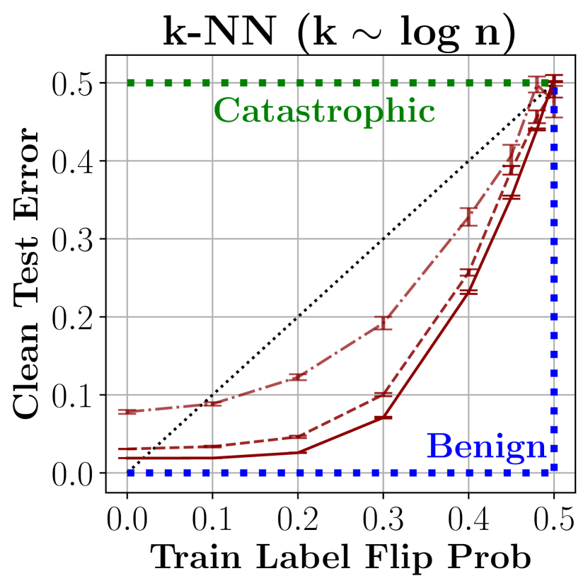
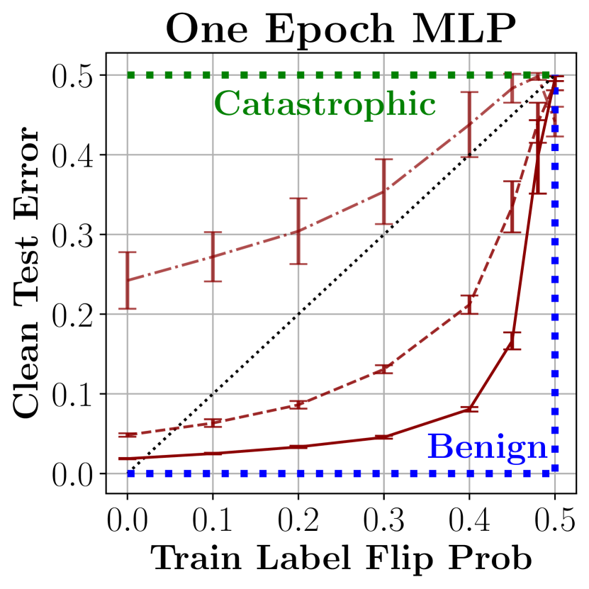
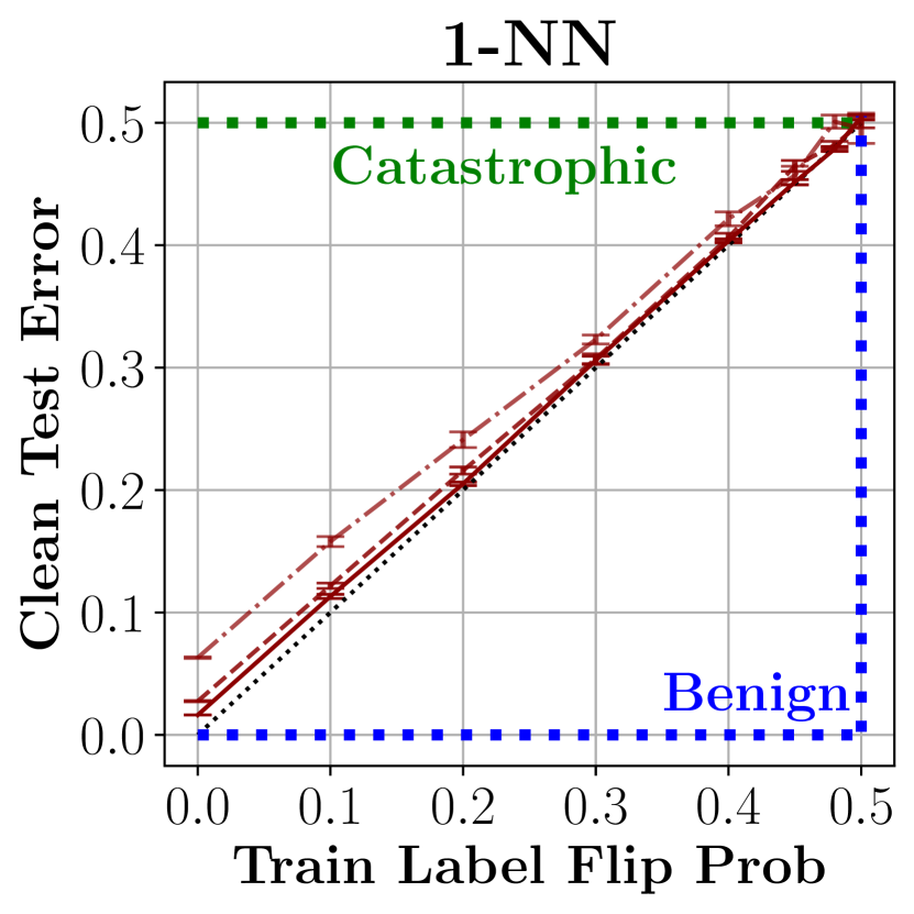
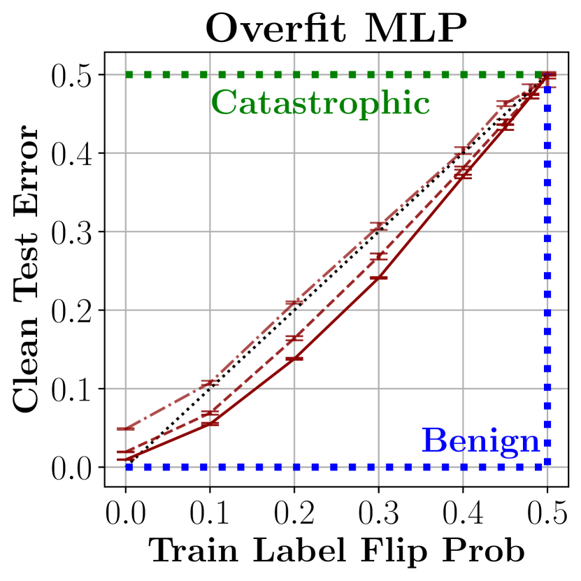
Figure 3: Examples of Benign and Tempered Fitting. Noise profiles for several different methods on the Binary-MNIST classification task, showing clean test error as a function of train label noise as the train set $n$ grows. Left: two methods which exhibit benign overfitting, with performance converging to Bayes optimal as $n\to\infty$. Right: two methods which exhibit tempered overfitting, with test error that remains bounded away from $0$. The two “tempered” methods here are interpolating, while the two “benign” methods are not. Both the benign and the tempered MLP use identical architectures; one is trained for one epoch, and the other trained to interpolation. Details in Appendix C.3.

2.3 Noise Profiles

To study asymptotic risk, we use a tool we call a noise profile. A noise profile characterizes the sensitivity of a learning procedure to noise in the training set. For a given learning procedure $\mathcal{A}$ and data distribution $\mathcal{D}$, a noise profile $\mathsf{P}_{\mathcal{A}}$ describes how the asymptotic risk varies with respect to $\sigma$, the level of artificial noise added to training targets. Formally, the noise profile $\mathsf{P}_{\mathcal{A}}$ is

$$\mathsf{P}_{\mathcal{A}}(\sigma)=\lim_{n\to\infty}\mathop{\mathbb{E}}_{A_{n};\mathcal{D}_{n}(\sigma)}R(A_{n}(D_{n}(\sigma))),$$ (1)

where $\mathcal{D}_{n}(\sigma)$ denotes $n$ i.i.d. samples from the distribution $\mathcal{D}$, with $\sigma$-level of label noise added. The label noise $\sigma\in\mathbb{R}$ denotes a kind of noise that depends on the problem setting: $\sigma$ is the variance of additive Gaussian noise for regression settings, or the label-flip probability for classification settings. We cannot empirically evaluate the $n\to\infty$ limit exactly, so we estimate it using asymptotics from finite but large sample sizes. As shown in Figure 2, noise profiles are easily plotted and reveal at a glance whether an learning procedure is benign, tempered, or catastrophic.

2.4 Applying Our Taxonomy

Benign	Tempered	Catastrophic
• Early-stopped DNNs • KR with ridge • $k$-NN ($k\sim\log n$) • Nadaraya-Watson kernel smoothing with Hilbert kernel	• Interpolating DNNs • Laplace KR • ReLU NTKs • $k$-NN (constant $k$) • Simplicial interpolation	• Gaussian KR • Critically-parameterized regression

Table 2: A taxonomy of models under the three types of fitting identified in this work. BOLD are results from our work, others are known or folklore results.

Our taxonomy handles general learning procedures, even those which do not interpolate their train sets. Thus, we can apply it to describe many existing methods in machine learning. In doing so, we refine the language around statistical consistency: many methods were known to be statistically inconsistent (i.e. not benign), but we highlight that there are two distinct ways to be inconsistent: tempered and catastrophic.

To illustrate our taxonomy, we give several examples of known results in Table 2. Any statistically consistent method is by definition benign: this includes non-interpolating methods such as early-stopped DNNs (Ji et al., 2021) and $k$-nearest-neighbors with $k\sim\log n$ (Cover and Hart, 1967; Chaudhuri and Dasgupta, 2014), as well as interpolating methods such as Nadarya-Watson kernel smoothing (Devroye et al., 1998) and k-NN schemes (Belkin et al., 2018a, 2019c).

Many catastrophic learning procedures are also known. Parametric models which are “critically-parameterized” (i.e. at the double descent peak) overfit catastrophically: this includes random feature regression with number of features $p=n$ (Mei and Montanari, 2019), and, more generally, for a broad class of linear and random feature methods (Holzmüller, 2021). Generic empirical-risk-minimization for a hypothesis class with VC-dimension $>n$ will also overfit catastrophically in the worst case. It turns out that RBF kernel regression under natural assumptions also catastrophically overfits, as we show in Section 3.

Finally, many methods, from classical to modern, exhibit tempered overfitting. First, it is well-known that 1-nearest-neighbors (1-NN) converges to an asymptotic risk that is finite but bounded away from Bayes optimal, which is tempered behavior. Further, any “underfitting” method, such as empirical risk minimization over a hypothesis class with VC-dimension $\ll n$, will be tempered if the hypothesis class does not contain the ground-truth function. In Section 4, we empirically demonstrate that many standard DNNs exhibit tempered overfitting when trained to interpolation. We complement this with theoretical results in Section 3, showing that kernel regression with the Laplace kernel, as well as with the ReLU NTK (which describes the training of an infinite-width ReLU fully-connected network (Jacot et al., 2018)), exhibits tempered overfitting. Our new category of tempered overfitting is thus not merely a theoretical possibility but in fact captures many natural and widely-used learning methods.

In Figure 3 we demonstrate our taxonomy experimentally for two benign methods ($k$-NN and early-stopped MLPs) and two tempered methods (1-NN and interpolating MLPs) on a binary classification version of MNIST, with varying noise in the train labels. We plot test classification error on the clean test set against the proportion of flipped labels in the training set. As $n$ grows, the benign methods approach zero test error even at nonzero train noise, while the tempered methods converge to a test error bounded away from zero.

3 Overfitting in Kernel Regression

We begin with a study of kernel regression (KR), a widely-used nonparameteric learning algorithm which, we will see, is sufficiently rich to exhibit all three regimes of overfitting, yet sufficiently simple that this can be shown analytically. Theoretical interest in this algorithm has increased significantly in recent years due to the discovery that trained DNNs converge to ridgeless KR in the infinite-width and infinite-time limit (Jacot et al., 2018), implying that insights into KR simultaneously shed light on overparameterized DNNs. The overparameterized linear regression setting of Bartlett et al. (2020) is equivalent to KR, and we will make a direct comparison with their results at the end of the section.

KR is fully specified by a positive-semidefinite kernel function $K:\mathbb{R}^{d}\times\mathbb{R}^{d}\rightarrow\mathbb{R}$ and a ridge parameter $\delta\geq 0$. We allow the training set $\mathcal{D}_{n}$ to contain $n$ samples $(x_{i},y_{i})\sim\mathcal{D}$, and we assume that $y_{i}=f^{*}(x_{i})+\eta_{i}$ with true function $f^{*}$ and noise $\eta_{i}\sim\mathcal{N}(0,\sigma^{2})$. KR returns the predicted function $\widehat{f}$ given by

$$\widehat{f}(x)=K(x,\mathcal{D}_{n})\left(K(\mathcal{D}_{n},\mathcal{D}_{n})+\delta\mathbf{I}_{n}\right)^{-1}\mathcal{Y},$$ (2)

where $K(\mathcal{D}_{n},\mathcal{D}_{n})$ is the “data-data kernel matrix” with components $K(\mathcal{D}_{n},\mathcal{D}_{n})_{ij}=K(x_{i},x_{j})$, $K(x,\mathcal{D})$ is a row vector with components $K(x,\mathcal{D})_{i}=K(x,x_{i})$, and $\mathcal{Y}$ is a column vector of target labels.

Existing literature provides examples of KR exhibiting all three asymptotic behaviors. Benign overfitting has been analyzed for overparameterized linear regression (Advani and Saxe, 2017; Bartlett et al., 2020; Muthukumar et al., 2020; Hastie et al., 2019; Belkin et al., 2019b), a special case of KR. It is well-known that KR with a positive ridge value (with appropriate scaling conventions) is consistent and thus benign (Christmann and Steinwart, 2007). Furthermore, in 1D, a Laplace kernel approaches piecewise linear interpolation as $n\rightarrow\infty$ (Belkin et al., 2018a), which is easily shown to exhibit tempered overfitting, and Rakhlin and Zhai (2019) proved that the Laplace kernel does not overfit benignly in (fixed) dimension greater than one (though did not say whether it was in fact tempered or catastrophic). Finally, it is known in experimental folklore (though not theoretically, to our knowledge) that KR with a Gaussian kernel and zero ridge tends to yield poorly-conditioned kernel matrices and catastrophic behavior. Here we derive fairly general conditions under which KR falls into each regime, solidifying these various observations into a unified picture.

As our chief tool for obtaining these conditions, we use a recently-derived closed-form approximation for the expected test MSE of KR (Bordelon et al., 2020; Canatar et al., 2021; Jacot et al., 2020; Simon et al., 2021). By simply taking the $n\rightarrow\infty$ limit of this expression, we can classify a given kernel into one of our three regimes.

The expression we will use gives test MSE in terms of the eigenspectrum of the kernel (as given by the Mercer decomposition) and the eigendecomposition of the target function. The nonnegative eigenvalues $\lambda_{1}\geq\lambda_{2}\geq...\geq 0$ and orthonormal eigenfunctions $\{\phi_{i}\}_{i=1}^{\infty}$ are given by

$$\mathbb{E}_{x^{\prime}\sim p}[K(x,x^{\prime})\phi_{i}(x^{\prime})]=\lambda_{i}\phi_{i}(x),\ \ \ \ \ \text{where}\ \ \ \ \mathbb{E}_{x\sim p}[\phi_{i}(x)\phi_{j}(x)]=\delta_{ij}.$$ (3)

We note that a kernel must be positive semidefinite and that $\sum_{i}\lambda_{i}=\text{Tr}[K]=\mathbb{E}_{x\sim p}[K(x,x)]$, which we assume is finite. Because the eigenfunctions form a complete basis, we are free to decompose the target function as $f^{*}(x)=\sum_{i}v_{i}\phi_{i}(x)$, where $\{v_{i}\}_{i=1}^{\infty}$ are eigencoefficients.

The above-mentioned works derive equivalent closed-form expressions for the test MSE of KR in terms of this spectral information using methods from the statistical physics literature. These methods are nonrigorous and rely on approximations (see Appendix A for a discussion), but they are expected to become exact in the large-$n$ limit, and comparison with empirical KR generally confirms a close match even at modest $n$. Here we use the framework of Simon et al. (2021), which expresses the final result in terms of “modewise learnabilities" $\{\mathcal{L}_{i}\}_{i=1}^{\infty}$, a set of scores in $[0,1]$ which indicate how well each eigenmode is learned at a given $n$. This choice of variables will simplify our proofs.

Simon et al. (2021) find that test MSE $\mathcal{R}_{n}$ is approximated by

$$\begin{split}\mathcal{R}_{n}&\approx\mathcal{E}_{n}\equiv\mathcal{E}_{0}\left(\sum_{i}(1-\mathcal{L}_{i})^{2}v_{i}^{2}+\sigma^{2}\right),\ \ \ \ \text{where}\ \ \ \ \mathcal{E}_{0}\equiv\frac{n}{n-\sum_{j}\mathcal{L}_{j}^{2}},\\ \mathcal{L}_{i}&\equiv\frac{\lambda_{i}}{\lambda_{i}+\kappa},\ \ \ \ \text{and}\ \ \ \ \kappa\geq 0\text{ satisfies }\sum_{i}\frac{\lambda_{i}}{\lambda_{i}+\kappa}+\frac{\delta}{\kappa}=n.\end{split}$$ (4)

This MSE includes noise on test labels; to instead compute a value for excess risk, one would simply subtract $\sigma^{2}$.

Here we study the asymptotic behavior of $\mathcal{E}_{n}$ as $n\rightarrow\infty$ for varying eigenspectra and ridge values. The fitting regime of the kernel is then given by this limit: (a) if $\lim_{n\rightarrow\infty}\mathcal{E}_{n}=\sigma^{2}$ (the Bayes-optimal MSE), then fitting is benign, (b) if $\lim_{n\rightarrow\infty}\mathcal{E}_{n}\in(\sigma^{2},\infty)$, then fitting is tempered, and (c) if $\lim_{n\rightarrow\infty}\mathcal{E}_{n}=\infty$, then fitting is catastrophic. We obtain conditions on the kernel eigenspectrum under which KR falls into each of these three regimes.

Our proofs rely on several (quite weak) technical assumptions on $\{\lambda_{i}\}_{i}$ and $\{v_{i}\}_{i}$, the most important of which is that the target function does not place weight in zero-eigenvalue modes (i.e. outside the kernel’s RKHS). We defer enumeration and discussion of these conditions to Appendix A, where they are listed as Assumption A.1. Our result is the following:

Theorem 3.1 (KR trichotomy).

For $\{\lambda_{i}\}_{i=1}^{\infty}$ and $\{v_{i}\}_{i=1}^{\infty}$ satisfying Assumption A.1, $\sigma^{2}>0$, and $\mathcal{E}_{n}$ given by Eq. 4,

1. If $\delta>0$ or $\lambda_{i}=i^{-1}\log^{-\alpha}i$ for some $\alpha>1$, then $\lim\limits_{n\rightarrow\infty}\mathcal{E}_{n}=\sigma^{2}$.

2. If $\delta=0$ and $\lambda_{i}=i^{-\alpha}$ for some $\alpha>1$, then $\lim\limits_{n\rightarrow\infty}\mathcal{E}_{n}=\alpha\sigma^{2}$.

3. If $\delta=0$ and $\lambda_{i}=i^{-\log i}$, or more generally if $\frac{\lambda_{i}}{\lambda_{i+1}}\geq\frac{i^{-\log i}}{(i+1)^{-\log(i+1)}}$ for all $i$, then $\lim\limits_{n\rightarrow\infty}\mathcal{E}_{n}=\infty$.

We defer the proof to Appendix A. The proof proceeds by first showing that asymptotic MSE is dominated by the noise, not the true function, and then computing $\lim_{n\rightarrow\infty}\mathcal{E}_{0}$ in each of the three cases.

Theorem 3.1 can be summarized as follows: a ridge parameter or extremely slow eigendecay leads to benign fitting, powerlaw decay of eigenvalues leads to tempered overfitting, and eigenvalue decay at least as fast as $i^{-\log i}$ leads to catastrophic overfitting. This theorem strongly suggests the satisfying heuristic that decay slower than any $\alpha>1$ powerlaw is benign, powerlaw decay itself is tempered, and decay faster than any powerlaw is catastrophic. As $\alpha$ grows in $(1,\infty)$, powerlaw spectra fully interpolate between benign and catastrophic, suggesting we have not missed any regime of interest to our taxonomy. The fact that the asymptotic MSE from a powerlaw spectrum is simply $\alpha\sigma^{2}$ is a pleasant surprise.

Theorem 3.1 has several consequences for KR with familiar kernels and the training of infinite-width networks. For illustrative purposes, we contrast the Gaussian (RBF) kernel $K_{G}(x_{1},x_{2})=e^{-w^{-2}|\!|x_{1}-x_{2}|\!|_{2}^{2}}$ with the Laplace kernel $K_{L}(x_{1},x_{2})=e^{-w^{-1}|\!|x_{1}-x_{2}|\!|_{2}}$, where $w$ is a bandwidth parameter. With data drawn from a $d$-dimensional manifold, the Gaussian and Laplace kernels have eigenspectra that decay like $\lambda_{i}\sim e^{-i^{2/d}}$ (as can be seen by taking a Fourier transform of $K_{G}$) and $\lambda_{i}\sim i^{-(d+1)/d}$ (Bietti and Bach, 2020), respectively. We note that ReLU NTKs, restricted to the hypersphere, have the same eigendecay as the Laplace kernel (Geifman et al., 2020; Chen and Xu, 2020). The implications of Theorem 3.1 include the following:

• KR with a fixed positive ridge parameter will fit any function in the kernel’s RKHS benignly as $n\rightarrow\infty$.

• Ridgeless KR with Laplace kernels or ReLU NTKs will exhibit tempered overfitting with $\Theta(1/d)$ excess MSE, approaching benignness as dimension grows.

• Ridgeless KR with the Gaussian kernel will exhibit catastrophic overfitting.

• The asymptotic behavior of KR with non-ReLU NTKs depends on the activation function. Virtually any kernel on the $d$-sphere (including the Gaussian kernel) can be realized as the NTK of a wide network with a proper choice of activation function (Simon et al., 2022), and thus there exist choices of activation function that yield catastrophic as well as tempered overfitting.

• Early stopping is known to act as an effective ridge parameter for wide networks (Ali et al., 2019), and thus we should expect that early-stopped wide networks will fit benignly.

We provide experiments illustrating Theorem 3.1 with Gaussian and Laplace kernels in Section 4. We additionally check Theorem 3.1b with several subsequent experiments: Figure 5 shows that, in synthetic KR with Gaussian eigenfunctions and exact powerlaw spectra, $\lim_{n\rightarrow\infty}\mathcal{E}_{n}$ is $\alpha\sigma^{2}$. And Figure 9 in Appendix B shows that, as predicted, Laplace kernels indeed appear to have asymptotic risk that decays like $\Theta(1/d)$.

We note that, to our knowledge, no well-known kernel has an eigendecay slower than all $\alpha>1$ powerlaws in finite dimension, and finding one in closed form — yielding ridgeless KR which overfits benignly — is an interesting open problem.

Comparison with Bartlett et al. (2020).

Our setting is essentially the same as the overparameterized linear regression setup studied by Bartlett et al. (2020): KR is equivalent to linear regression in eigenfeature space, and our kernel eigenvalues are equivalent to their covariance matrix eigenvalues. Our spectral condition for benignness in Theorem 3.1a is precisely that of their Theorem 6.1, and we include it for completeness. Their Theorem 6.1 notes that powerlaw decays with $\alpha>1$ are not benign; here we find that they are in fact tempered.

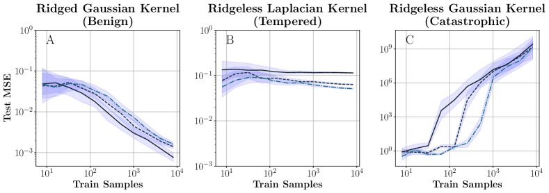
Figure 4: Kernel regression can exhibit all three fitting regimes with proper choice of ridge parameter and kernel. Plots show learning curves for KR with data $\{x_{i}\}$ sampled uniformly from the unit sphere $\mathcal{S}^{d-1}$, trained with pure noise target labels $y_{i}\sim\mathcal{N}(0,1)$. Test MSE is computed with respect to a clean test set. (a) KR with a Gaussian kernel and nonzero ridge is asymptotically benign. A ridge value of $\delta=0.1$ was used. (b) Ridgeless KR with a Laplace kernel exhibits tempered overfitting. (c) Ridgeless KR with a Gaussian kernel exhibits catastrophic overfitting.

4 Experiments

Having demonstrated the three types of fitting theoretically in KR, we now present a series of experimental results illustrating these regimes in both KR and deep neural networks (DNNs). We show results on various common datasets and models to give evidence that these phenomena are not specific to our particular theoretical setting, but are widely relevant across machine learning. First, we empirically verify Theorem 3.1 through simple synthetic experiments with ridged kernels, and the ridgeless Laplace and Gaussian kernel. We see these three choices of kernels exhibit the three different regimes of overfitting, exactly as predicted by our theorem. This confirms both that our theoretical heuristics (which were nonrigorous in places) are empirically accurate, and that the asymptotic behavior is evident at realistically large sample sizes.

We then perform similar regression and classification experiments using MLPs, to show that, beyond the kernel setting, simple DNNs can also exhibit both benign and tempered overfitting — depending on the early-stopping criteria. We provide full experimental details in Appendix C.

4.1 Experiments on Kernel Regression

In Figure 4, we run KR on the following synthetic data distribution: the inputs $x$ are sampled from the unit sphere $\mathcal{S}^{d-1}$, and the targets $y$ are zero-mean Gaussian noise ($y\sim\mathcal{N}(0,1)$). This is an extremely simple regression setting: we are just trying to learn the constant-$0$ function under Gaussian observation noise. We run KR with three choices of kernel: (A) Gaussian kernel with ridge, (B) Laplace kernel without ridge, and (C) Gaussian kernel without ridge. Figure 4 shows that as we increase the sample size, these three settings exhibit benign, tempered, and catastrophic behavior. This agrees with the spectral predictions of Theorem 3.1.

Interestingly, Figure 4c shows that increasing input dimension tends to both improve MSE at fixed sample size $n$, and increase the “critical” $n$ at which MSE begins to diverge. This suggests that high dimensionality can be a “blessing” which prevents catastrophic methods from diverging, agreeing with the spirit of prior work on the blessings of dimensionality for interpolating methods (e.g. (Rakhlin and Zhai, 2019)).

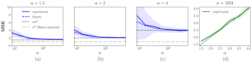
Figure 5: As $n$ grows, the MSE of KR with Gaussian eigenfunctions and powerlaw kernel eigenspectra with exponent $\alpha$ approaches $\alpha\sigma^{2}$. (a-c): learning curves with different $\alpha$. (d): test MSE at $n=1024$ for varying $\alpha$, with the identity function shown by the solid line.

In Figure 5 we explore in more detail the dependency between a powerlaw kernel’s spectral decay rate and its asymptotic risk. We follow the same train and test setup for these experiments, but construct special kernels such that their spectrum is precisely a powerlaw with exponent $\alpha$ and their eigenfunctions are indeed random Gaussians. This experimental setup, described in full in Appendix B, is equivalent to linear regression with random Gaussian covariates and a covariance kernel with known spectrum. We see that as the spectral decay $\alpha$ varies, the (asymptotic) test MSE varies as approximately $\alpha\sigma^{2}$, agreeing with part (b) of Theorem 3.1.

4.2 Experiments on Deep Neural Networks

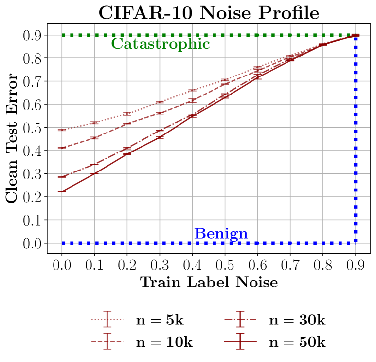
(a) WideResNet trained on CIFAR-10.

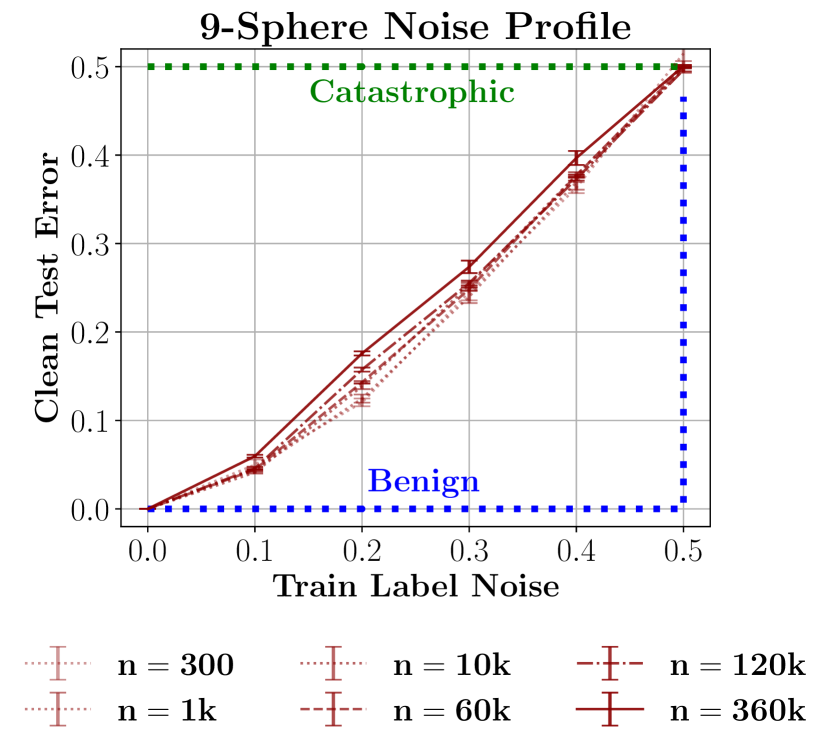
(b) MLP trained on the constant function.

Figure 6: Noise profiles for interpolating DNNs on CIFAR-10 and synthetic classification tasks. In both settings, the noise profiles asymptotically behave as tempered overfitting: neither catastrophic nor benign.

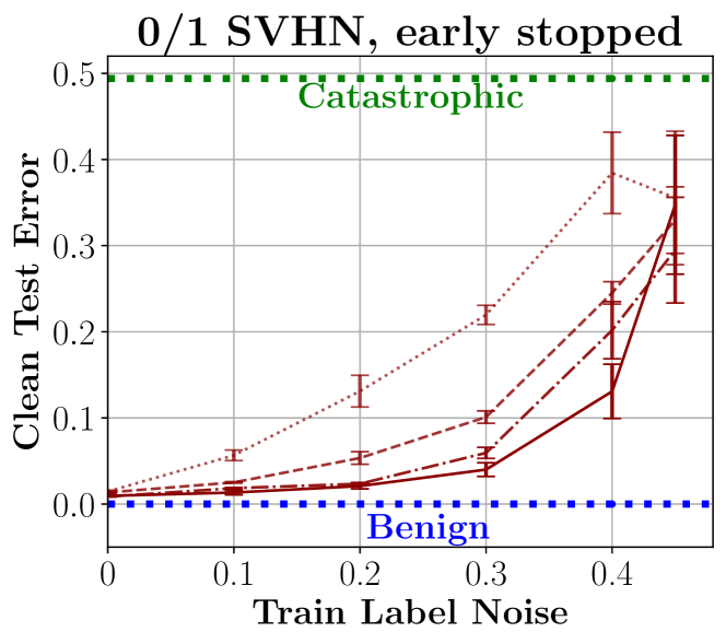
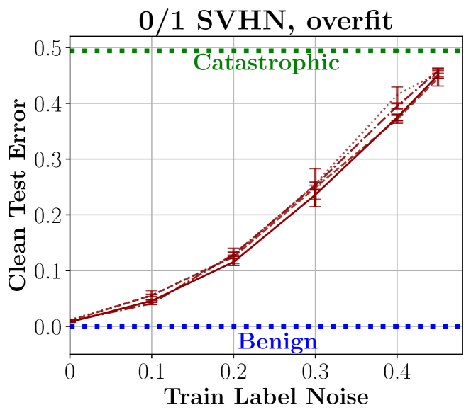
Figure 7: Early-stopped DNNs exhibit fairly benign fitting, while DNNs trained to interpolation exhibit tempered overfitting. We show noise profiles for ResNets trained on Binary SVHN (0/1 digit classification). (a) With early stopping, noise profiles approach zero test error as $n$ increases, even with finite label noise, indicating benign fitting. (b) When training to interpolation, noise profiles converge to a limiting, roughly linear curve as $n$ increases, indicating tempered fitting.

Interpolating DNNs.

Figure 2 and Figure 6(a) show the noise profiles for ResNets trained to interpolation on two-class and ten-class versions of CIFAR-10, respectively. In both settings, interpolating DNNs do not approach Bayes optimality, and instead exhibit tempered overfitting. This tempered behavior is widespread across even much simpler DNN settings. For example, in Figure 6(b), we train a three-layer interpolating MLP for binary classification on an extremely simple synthetic dataset: with inputs drawn from $\mathcal{S}^{9}$ and ground-truth labels as the constant function $f^{*}(x)=1$. Even in this simple setting, at large sample size, interpolating DNNs are not benign—they do not successfully learn the constant function in the presence of even slight label noise. Note that although this experiment is outside the technical scope of Theorem 3.1, it is heuristically consistent: wide ReLU MLPs tend to have NTKs with powerlaw spectra, and thus will exhibit tempered overfitting when trained in the NTK regime.

Early-stopped DNNs.

We now consider DNNs that have been optimally early-stopped. Figure 7 shows noise profiles for Wide ResNets trained on a binary version of SVHN, both stopped early (Figure 7a) and trained to interpolation (Figure 7b). The early-stopped ResNets approach benign fitting as $n$ grows, with low error even at sizable noise levels, while the ResNets trained to interpolation quickly converge to a tempered noise profile. This mirrors the behavior of MLPs on binary MNIST, after one epoch of training and after interpolation, shown earlier in Figure 3. Although these benign DNN results are outside the formal scope of known theoretical results, it is heuristically consistent with results such as Ji et al. (2021), which show that certain wide and shallow ReLU MLPs are consistent when early-stopped.

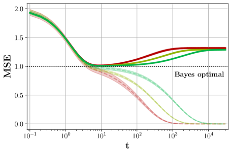
Figure 8: MLPs trained on noisy data fit benignly at early times and exhibit tempered overfitting at late times. Curves show train and test MSE for a $4\times 500$ ReLU MLP with target labels $y_{i}\sim\mathcal{N}(1,1)$ and varying trainset size $n$. Benign fitting, with near-Bayes-optimal test MSE, begins around $t=3$, ending as the network begins to fit the noise in the training set. Tempered overfitting is reflected in the suboptimal-but-finite asymptotic test MSE as $t$ becomes large.

Time dynamics.

The above discussion suggests that as a single DNN is trained, it exhibits benign fitting early in training (when it has not fit the noise in its train set), and then transitions to tempered overfitting late in training (as it eventually fits the noise). In Figure 8, we show a simple experiment that illustrates these time dynamics. We train a ReLU MLP on the following synthetic regression task (similar to Figure 6(b)): The inputs $x$ are sampled from the unit sphere $\mathcal{S}^{4}$, and the targets are $\mathcal{N}(1,1)$. That is, we are simply trying to learn the constant function $f^{*}(x)=1$ on the unit sphere, with Gaussian observation noise. We then plot the test MSE as a function of the number of optimization steps taken.

From Figure 8, we see that for all train sizes $n$, the network quickly reaches nearly Bayes-optimal test performance early in training. In this initial fitting phase, train and test MSE decrease together: the network is fitting the ground-truth function but has not yet fit the noise. Once the train MSE drops below the Bayes risk, however, the dynamics change. At this point (around time $t=4$ in Figure 8), the network must start to fit noise in the train set, since the train loss drops below the optimal possible test loss. As training continues, we see the train loss decrease, but the test loss increase for the remainder of training: fitting noise in the train set hurts test performance. Finally, in the limit of large time $t$, the network converges to a test loss that is tempered: above Bayes-optimal, but asymptotically constant as a function of samples $n$.

Remark on Shape of Profiles.

The fact that noise profiles for classification all seem to approach lines with slope one is is not at all trivial — many alternate profile shapes are a priori possible. This empirical observation was formalized in Nakkiran and Bansal (2020), but remains theoretically open to understand. In the KR setting, Theorem 3.1b states that test error will indeed be proportional to target noise, but the proportionality constant will generally be smaller than one. We suggest this difference in noise sensitivity is one important difference between classification and regression.

5 Limitations

In this paper, we have presented a taxonomy of overfitting, presented empirical evidence that DNNs trained to interpolation exhibit tempered overfitting, and identified spectral conditions under which KR, a toy model for DNNs, falls into each regime. This is a first study into this regime, and many questions await careful exploration. We detail several here.

First, our DNN results are entirely empirical, and there is room for complementary theoretical studies into the overfitting regimes of shallow networks and wide networks with NTK and mean-field parameterization. Second, while we have used several real and synthetic datasets, all are of at most moderate size, and a study at large scale — using correspondingly large models — is potentially interesting. Third, we have found that in some realistic settings, interpolating DNNs are tempered, but it remains open whether there might exist settings or tasks for which interpolating DNNs overfit benignly or catastrophically. Fourth, Theorem 3.1 required a “universality” assumption which ought to be checked for each kernel. Finally, our KR results suggest that input or manifold dimension should play a role in the degree of tempered overfitting, and the effect of dimensionality on overfitting is yet to be disentangled.

6 Conclusion

In this paper we study the nature of overfitting in learning methods which interpolate their training data. Much of contemporary theory and experimental work categorizes overfitting as either catastrophic or benign. In contrast, we observe that many natural learning procedures, including DNNs used in practice, overfit in a manner that is neither benign nor catastrophic— but rather in an intermediate regime. We identify and formally define this regime, which we call tempered overfitting. We present empirical evidence of learning procedures that exhibit tempered overfitting, on both synthetic and natural data, using kernel machines and deep neural networks. We show tempered overfitting can be quantified in terms of noise profiles, which measure how asymptotic performance depends on noise in the train distribution. For kernel regression, we provide a theoretical result in the form of a trichotomy: conditions on problem parameters which yield each of the three regimes of overfitting.

Our work presents an initial study of tempered overfitting and lays the framework for future study of what we believe is a rich and relevant regime for modern learning. We hope this framework inspires further investigation into tempered overfitting for more complex models, both theoretically and experimentally. For example, it is open to understand which conditions on neural network architecture, training hyperparameters and data distribution lead to benign, tempered, or catastrophic overfitting, in analogy to our “kernel trichotomy”, and an answer might shed light on practical DNNs.

Acknowledgments

The authors thank Nikhil Ghosh, Annabelle Carrell, Spencer Frei, Daniel Beaglehole, Gil Kur, and Russ Webb for useful discussion and feedback on the manuscript. JS additionally thanks two strangers on a DC Metro for useful discussion. PN especially thanks the Simons Institute, UCSD, and Apple MLR for collaborative environments which made this project possible.

We are grateful for support from the National Science Foundation (NSF) and the Simons Foundation for the Collaboration on the Theoretical Foundations of Deep Learning through awards DMS-2031883 and #814639 as well as NSF IIS-1815697 and the TILOS institute (NSF CCF-2112665). NM is thankful to be funded and supported for this research by the Eric and Wendy Schmidt Center. JS gratefully acknowledges support from the NSF Graduate Fellow Research Program (NSF-GRFP) under grant DGE 1752814. This work used the Extreme Science and Engineering Discovery Environment (XSEDE) (Towns et al., 2014), which is supported by NSF grant number ACI-1548562, Expanse CPU/GPU compute nodes, and allocations TG-CIS210104 and TG-CIS220009.

Author Contributions

NM developed and performed the bulk of the experiments, drafted the initial version of the manuscript, actively contributed to writing and editing, and led the team logistically. JS proposed and proved the theoretical KR results, aided in experimentation, and contributed to the writing throughout the paper. AA developed and executed most of the kernel experiments, provided support to other experiments, and helped edit the manuscript. PP and MB provided guidance for experiments and theory, and reviewed and edited drafts of the manuscript. PN initiated this research agenda and provided active input throughout the experimentation, theory, and writing phases of the project.

Appendix A Proof of Theorem 3.1: KR Trichotomy

In this appendix, we provide proofs and further discussion of our theoretical results for KR. To aid readers, we begin by reproducing Equation 4 for the approximate generalization MSE of KR:

$$\begin{split}\mathcal{E}\approx\mathcal{E}_{0}\left(\sum_{i}(1-\mathcal{L}_{i})^{2}v_{i}^{2}+\varepsilon^{2}\right),\ \ \ \ \text{where}\ \ \ \ \mathcal{E}_{0}\equiv\frac{n}{n-\sum_{j}\mathcal{L}_{j}^{2}},\\ \mathcal{L}_{i}\equiv\frac{\lambda_{i}}{\lambda_{i}+\kappa},\ \ \ \ \text{and}\ \ \ \ \kappa\geq 0\text{ satisfies }\sum_{i}\frac{\lambda_{i}}{\lambda_{i}+\kappa}+\frac{\delta}{\kappa}=n.\end{split}$$ (4)

The works obtaining this result [Bordelon et al., 2020, Canatar et al., 2021, Jacot et al., 2020, Simon et al., 2021] make certain approximations common in the statistical physical literature. The main one is the universality assumption that the eigenfunctions can be replaced by structureless Gaussian random variables without changing the statistics of test risk (see Jacot et al. [2020] for a formalization of this assumption). Though this step discards most of the information in the problem (leaving only the scalar eigenvalues and eigencoefficients), it is validated by the close match between experiment and the theory derived with this approximation. KR is equivalent to linear regression in the high-dimensional kernel embedding space defined by its eigenfeatures, and we note several recent works which have derived the same equations for high-dimensional linear regression, analogously assuming i.i.d. random covariates [Hastie et al., 2019, Bartlett et al., 2021]. This assumption of i.i.d. random covariates is also made by Bartlett et al. [2020].

In studying these equations, we assume the following:

Assumption A.1.

The kernel eigenvalues $\{\lambda_{i}\}_{i=1}^{\infty}$ and target function eigencoefficients $\{v_{i}\}_{i=1}^{\infty}$ satisfy

1. $\lambda_{i}>\lambda_{j}$ if $i>j$,

2. $\sum\limits_{i=1}^{\infty}\lambda_{i}<\infty$,

3. $\{\lambda_{i}\}_{i=1}^{\infty}$ contains infinitely many nonzero elements,

4. $\sum\limits_{i=1}^{\infty}v_{i}^{2}<\infty$, and

5. $\lim\limits_{\lambda\rightarrow 0^{+}}\sum\limits_{i|\lambda_{i}<\lambda}v_{i}^{2}=0$.

These natural assumptions imply that (a) we have indexed the eigenvalues in descending order, (b) the trace of the kernel is finite, (c) the rank of the kernel is infinite (which is typically the case in practice), (d) the target function has finite $\ell^{2}$-norm, and (e) the target function does not place non-negligible weight in arbitrarily-low (or zero) eigenmodes. While condition (e) is somewhat nonstandard, we note that it is strictly weaker than requiring finite RKHS norm of $f$ w.r.t. $K$:

$$|\!|f|\!|_{K}^{2}=\sum_{i=1}^{\infty}\frac{v_{i}^{2}}{\lambda_{i}}<\infty.$$ (5)

We note that all eigenvalues are nonnegative because the kernel is positive semidefinite.

The constant $\kappa$ fixed by Equation 4 satisfies

$$\kappa \leq\frac{1}{n\gamma}\left(\delta+\sum_{i\geq n(1-\gamma)}\lambda_{i}\right),$$ (6)

$$\kappa \geq\gamma\lambda_{n(1+\gamma)},$$ (7)

where $\gamma\in(0,1)$ in Equation 6, $\gamma\in(0,\infty)$ in Equation 7, and in both cases $\gamma$ satisfies $\gamma n\in\mathbb{Z}$. These bounds follow from more general bounds in Simon et al. [2021]. We will use them shortly.

Proof of Theorem 3.1. We begin by observing from Equation 6 with any $\gamma\in(0,1)$ that $\kappa=\mathcal{O}(1/n)$, and thus $\lim_{n\rightarrow\infty}\kappa=0$ and $\lim_{n\rightarrow\infty}\mathcal{L}_{i}=1$ if $\lambda_{i}$ is bounded away from 0. Paired with Assumption A.1e, this implies that $\lim_{n\rightarrow\infty}\sum_{i}(1-\mathcal{L}_{i})^{2}v_{i}^{2}=0$, and thus, examining Equation 4, we find that asymptotic MSE is dominated by the noise $\varepsilon^{2}$ and given by

$$\lim_{n\rightarrow\infty}\mathcal{E}=\left(\lim_{n\rightarrow\infty}\mathcal{E}_{0}\right)\varepsilon^{2}.$$ (8)

Asymptotic MSE is thus dominated by the noise, and we can neglect the target coefficients $\{v_{i}\}_{i}$.

We now prove each clause of the theorem by finding $\lim\limits_{n\rightarrow\infty}\mathcal{E}_{0}$, beginning with the two parts of clause (a).

Clause (a): if $\delta>0$, then $\lim\limits_{n\rightarrow\infty}\mathcal{E}=\varepsilon^{2}$.

We assume that $\delta>0$. To begin, we note a lower bound for $\kappa$. Since

$$n=\sum_{i=1}^{\infty}\frac{\lambda_{i}}{\lambda_{i}+\kappa}+\frac{\delta}{\kappa}\geq\frac{\delta}{\kappa},$$ (9)

it follows that $\kappa\geq\delta/n$. Using this bound, we find that

$$\frac{1}{n}\sum_{i=1}^{\infty}\mathcal{L}_{i}^{2}=\frac{1}{n}\sum_{i=1}^{\infty}\frac{\lambda_{i}^{2}}{(\lambda_{i}+\kappa)^{2}}\leq\gamma+\frac{1}{n}\sum_{i\geq n\gamma}\frac{\lambda_{i}^{2}}{\kappa^{2}}\leq\gamma+n\sum_{i\geq n\gamma}\frac{\lambda_{i}^{2}}{\delta^{2}},$$ (10)

where $\gamma\in(0,1)$ and we have “given up" on the first $\gamma n$ terms in the sum, replacing them with 1.

Because $\sum_{i=1}^{\infty}\lambda_{i}<\infty$, it must hold that $\lambda_{i}=o(i^{-1})$, and thus the sum on the far RHS of Equation 10 approaches zero as $n\rightarrow\infty$. This tells us that $\lim_{n\rightarrow\infty}\mathcal{E}_{0}=\lim_{n\rightarrow\infty}n/(n+\sum_{i}\mathcal{L}_{i}^{2})\leq 1/(1+\gamma)$. By choosing $\gamma$ to be arbitrarily small, we can push this bound to $1$, which proves the clause.

Clause (a’): if $\lambda_{i}=i^{-1}\log^{-\alpha}i$ for some $\alpha>1$, then $\lim\limits_{n\rightarrow\infty}\mathcal{E}=\varepsilon^{2}$.

We first set $\gamma=1$ in Equation 7 and find that $\kappa\geq\lambda_{2n}=(2n)^{-1}\log^{-\alpha}(2n)$. Anticipating our next move, we then note that, if $i\geq n$,

$$\kappa i\log^{\alpha}i\geq\frac{\log^{\alpha}n}{2(\log^{\alpha}n+\log^{\alpha}2)}\geq\frac{1}{5}\ \ \ \ \ \text{for sufficiently large $n$}.$$ (11)

We then observe that

$$n=\sum_{i=1}^{\infty}\frac{1}{1+\kappa i\log^{\alpha}i}\geq\sum_{i\geq n}\frac{1}{1+\kappa i\log^{\alpha}i}\geq\frac{1}{6\kappa}\sum_{i\geq n}\frac{1}{i\log^{\alpha}i}\geq\frac{1}{6\kappa}\frac{1}{(\alpha-1)\log^{\alpha-1}n},$$ (12)

where in the third step we have used Equation 11 and in the fourth step we have used the fact that $\int_{x}^{\infty}z^{-1}\log^{-\alpha}zdz=(\alpha-1)^{-1}\log^{-\alpha+1}x$. This tells us that

$$\kappa\geq\left(6(\alpha-1)n\log^{\alpha-1}n\right)^{-1}.$$ (13)

We then observe that

$$\sum_{i=1}^{\infty}\mathcal{L}_{i}^{2}\leq\frac{n}{\log\log n}+\sum_{i\geq\frac{n}{\log\log n}}\frac{\lambda_{i}^{2}}{\kappa^{2}}=\frac{n}{\log\log n}+\kappa^{-2}\Theta\left(\frac{\log\log n}{n\log^{2\alpha}n}\right),$$ (14)

where in the first step we have “given up" on the first $\frac{n}{\log\log n}$ terms and in the second step we have used the fact that $\int_{x}^{\infty}z^{-2}\log^{-2\alpha}zdz\xrightarrow[]{\text{large }x}x^{-1}\log^{-2\alpha}x$. Plugging in Equation 13, we find that the RHS of Equation 14 approaches $\frac{n}{\log\log n}$ at large $n$, and is thus $o(n)$. This implies benignness as in the proof of clause (a).

Clause (b): if $\delta=0$ and $\lambda_{i}=i^{-\alpha}$ for some $\alpha>1$, then $\lim\limits_{n\rightarrow\infty}\mathcal{E}_{0}=\alpha$.

The desired limit follows from direct computation upon replacing the sum over eigenvalues in the definition of $\kappa$ with an integral. To make the result rigorous, we shall simply bound this sum between two integrals.

The constant $\kappa$ satisfies

$$\sum_{i=1}^{\infty}\frac{i^{-\alpha}}{i^{-\alpha}+\kappa}=\sum_{i\geq 1}^{\infty}\frac{1}{1+\kappa i^{\alpha}}=n.$$ (15)

Noting that the summand decreases monotonically with $i$, we find that

$$n=\sum_{i=1}^{\infty}\frac{1}{1+\kappa i^{\alpha}}\geq\int_{1}^{\infty}\frac{di}{1+\kappa i^{\alpha}}\geq\int_{0}^{\infty}\frac{di}{1+\kappa i^{\alpha}}-1$$ (16)

and

$$n=\sum_{i=1}^{\infty}\frac{1}{1+\kappa i^{\alpha}}\leq\int_{0}^{\infty}\frac{di}{1+\kappa i^{\alpha}}.$$ (17)

It follows that $\kappa_{-}\leq\kappa\leq\kappa_{+}$, where $\kappa_{-}$ and $\kappa_{+}$ satisfy

$$\int_{0}^{\infty}\frac{di}{1+\kappa_{-}i^{\alpha}} =n+1,$$ (18)

$$\int_{0}^{\infty}\frac{di}{1+\kappa_{+}i^{\alpha}} =n.$$ (19)

Using the fact that $\int_{0}^{\infty}(1+x^{\alpha})^{-1}dx=\alpha^{-1}\pi\csc(\pi/\alpha)$ when $\alpha>1$, we find that

$$\kappa_{-}=\left[\frac{\pi}{\alpha}\csc(\pi/\alpha)\right]^{\alpha}n^{-\alpha},$$ (20)

$$\kappa_{+}=\left[\frac{\pi}{\alpha}\csc(\pi/\alpha)\right]^{\alpha}(n+1)^{-\alpha}.$$ (21)

These bounds converge as $n\rightarrow\infty$, and thus asymptotically $\kappa\rightarrow\left[\frac{\pi}{\alpha}\csc(\pi/\alpha)\right]^{\alpha}n^{-\alpha}$.

A similar argument using the integral $\int_{0}^{\infty}(1+x^{\alpha})^{-2}dx=\alpha^{-2}(\alpha-1)\pi\csc(\pi/\alpha)$ yields that

$$\sum_{i=1}^{\infty}\mathcal{L}_{i}^{2}\approx\int_{0}^{\infty}\frac{di}{(1+\kappa i^{\alpha})^{2}}\rightarrow\kappa^{-1/\alpha}\frac{\alpha-1}{\alpha^{2}}\pi\csc(\pi/\alpha)\rightarrow n\frac{\alpha-1}{\alpha},$$ (22)

where in the last step we have inserted our asymptotic expression for $\kappa$. We now find that $\mathcal{E}_{0}=\frac{n}{n-\sum_{i}\mathcal{L}_{i}^{2}}\rightarrow\alpha$.

Clause (c): if $\delta=0$ and $\frac{\lambda_{i}}{\lambda_{i+1}}\geq\frac{i^{-\log i}}{(i+1)^{-\log(i+1)}}$ for all $i$, then $\lim\limits_{n\rightarrow\infty}\mathcal{E}_{0}=\infty$.

We begin by observing that

$$\frac{1}{\mathcal{E}_{0}}=\frac{1}{n}\left(n-\sum_{j}\mathcal{L}_{j}\right)=\frac{1}{n}\sum_{j}\mathcal{L}_{j}(1-\mathcal{L}_{j})\leq\frac{1}{n}\sum_{i\leq n}(1-\mathcal{L}_{i})+\frac{1}{n}\sum_{i>n}\mathcal{L}_{i}.$$ (23)

We shall show that both terms on the RHS of Equation 23 approach zero as $n\rightarrow\infty$, and thus $\mathcal{E}_{0}$ diverges.

Considering the first term first, we note that

$$\frac{1}{n}\sum_{i\leq n}(1-\mathcal{L}_{i})=\frac{1}{n}\sum_{i\leq n}\frac{\kappa}{\lambda_{i}+\kappa} \stackrel{{\scriptstyle\mathclap{\tiny\mbox{(1)}}}}{{\leq}}\gamma+\frac{\kappa}{n}\!\!\!\sum_{i\leq n(1-\gamma)}\!\!\frac{1}{\lambda_{i}}$$ (24)

$$\leq\gamma+\frac{\kappa}{\lambda_{n(1-\gamma)}}\stackrel{{\scriptstyle\mathclap{\tiny\mbox{(2)}}}}{{\leq}}\gamma+\frac{1}{n\gamma}\sum_{i\geq n(1-\gamma)}\frac{i^{-\log i}}{(n(1-\gamma))^{-\log(n(1-\gamma))}},$$ (25)

where in step (1) we have ignored the last $n\gamma$ terms of the sum, and also used the fact that $\kappa/(\lambda_{i}+\kappa)\leq\kappa/\lambda_{i}$, and in step (2) we have used Equation 6 to upper-bound $\kappa$, with $\gamma$ a constant parameter we will later take to be small. Fixing $\gamma$ and taking $n\rightarrow\infty$, the final RHS of Equation 24 approaches $\gamma$. By making $\gamma$ arbitrarily small, we can make this upper bound approach zero.

Now examining the second term in Equation 23, we observe that

$$\frac{1}{n}\sum_{i>n}\mathcal{L}_{i}=\frac{1}{n}\sum_{i>n}\frac{\lambda_{i}}{\lambda_{i}+\kappa}\stackrel{{\scriptstyle\mathclap{\tiny\mbox{(1)}}}}{{\leq}}\gamma+\frac{1}{n\kappa}\sum_{i>n(1+\gamma)}\lambda_{i}\\ \stackrel{{\scriptstyle\mathclap{\tiny\mbox{(2)}}}}{{\leq}}\gamma+\frac{1}{n\gamma\lambda_{n(1+\gamma)}}\sum_{i>n(1+\gamma)}\lambda_{i}\leq\gamma+\frac{1}{n\gamma}\sum_{i\geq n(1+\gamma)}\frac{i^{-\log i}}{(n(1+\gamma))^{-\log(n(1+\gamma))}},$$ (26)

where in step (1) we have again “given up" on $n\gamma$ terms of the sum and in step (2) we have used Equation 7 to lower-bound $\kappa$. Using the same argument as above, the final RHS of Equation 26 approaches $\gamma$, which can be made arbitrarily small.

Combining subresults and looking again at Equation 23, we find that $\lim_{n\rightarrow\infty}\mathcal{E}_{0}^{-1}$ can be given an arbitrarily small upper-bound, and thus $\lim_{n\rightarrow\infty}\mathcal{E}_{0}=\infty$, which proves the clause. ∎

Remarks on proofs and proof techniques. Clause (a) shows that fitting is benign if $\delta>0$, but it is not hard to show that fitting is also benign if $\delta=0$ and instead $\delta^{\prime}\equiv\lim_{j\rightarrow\infty}\sum_{i\geq j}\lambda_{i}>0$. This odd tailsum $\delta^{\prime}$ can be shown to act like an effective ridge parameter in Equation 4, but with $\delta=0$ the resulting kernel interpolates the data. One way to add such an effective ridge to a kernel $K$ is to replace it with $K^{\prime}(x_{1},x_{2})\equiv K(x_{1},x_{2})+\delta^{\prime}\mathbbm{1}_{x_{1}=x_{2}}$, which (assuming train and test sets are disjoint) simply adds a ridge parameter $\delta^{\prime}$ to Equation 2 defining KR. The fact that many small eigenvalues can act like a ridge parameter is proven by and used in the derivations of Simon et al. [2021].

When proving clause (c), we used a ratio condition to capture the notion of super-powerlaw decay. We found that this ratio condition easier to work with than the weaker requirement that $\lambda_{i}=\mathcal{O}(i^{-\log i})$. We note that there was nothing special in the choice of $i^{-\log i}$, and any slower super-powerlaw decay, like $i^{-\log\log i}$, would have also sufficed.

Appendix B Powerlaw and Laplace kernel experiments

In Section 3 of the main text, we show via Theorem 3.1 that KR with a kernel with a powerlaw spectrum with exponent $\alpha$ overfits target noise by a factor $(\alpha-1)$ as $n\rightarrow\infty$, and we conclude that Laplace kernels, which are known to have powerlaw spectral tails, ought to obey this rule. Here we provide experimental evidence for both these claims.

We start with KR with a powerlaw spectrum. No simple kernel + domain pair gives an exact powerlaw spectrum $\lambda_{i}=i^{-\alpha}$, so we perform a synthetic experiment with Gaussian random eigenfunctions, which is essentially linear regression with random features as in the setting of Bartlett et al. [2020]. Letting $n$ denote the number of train samples, $n^{\prime}$ denote the number of test samples, and $M\gg n$ denote the number of eigenmodes (a.k.a. features), we first sample train and test feature matrices $\Phi\in\mathbb{R}^{M\times n}$ and $\Phi^{\prime}\in\mathbb{R}^{M\times n^{\prime}}$ with entries drawn i.i.d. from $\mathcal{N}(0,1)$. We then construct the train-train and test-train kernels as $K_{\text{tr-tr}}=\Phi^{T}\Lambda\Phi$ and $K_{\text{te-tr}}=\Phi^{\prime T}\Lambda\Phi$, respectively, where $\Lambda\equiv\text{diag}(\lambda_{1},\cdots,\lambda_{M})$ with $\lambda_{i}=i^{-\alpha}$.

The train and test targets are given by $\mathcal{Y}_{\text{tr}}=\Phi^{T}\mathbf{v}+\eta_{\text{tr}}$ and $\mathcal{Y}_{\text{te}}=\Phi^{\prime T}\mathbf{v}+\eta_{\text{te}}$, respectively, where $\mathbf{v}\in\mathbb{R}^{M}$ is a vector of target eigencoefficients and the noise vectors are sampled $\eta_{\text{tr}}\sim\mathcal{N}(0,\sigma^{2}\mathbf{I}_{n})$ and $\eta_{\text{tr}}\sim\mathcal{N}(0,\sigma^{2}\mathbf{I}_{n^{\prime}})$. The predicted test labels are computed via KR as $\widehat{\mathcal{Y}}_{\text{te}}=K_{\text{te-tr}}K_{\text{tr-tr}}^{-1}$ and the MSE is then $\frac{1}{n^{\prime}}|\mathcal{Y}_{\text{te}}-\widehat{\mathcal{Y}}_{\text{te}}|^{2}$.

We run experiments varying $n$ and using $n^{\prime}=3000$, $M=10^{4}$, $\mathbf{v}_{i}\sim i^{-2}$ normalized so $\sum_{i=1}^{M}\mathbf{v}_{i}^{2}=10$, $\sigma^{2}=1$, and varying $\alpha$. The results, shown in Figure 5, confirm that, as $n$ grows, MSE approaches $\alpha\sigma^{2}$ in accordance with Theorem 3.1b.

We now study proper KR with a Laplace kernel and data sampled i.i.d. from the hypersphere $\mathcal{S}^{d}\equiv\{x\in\mathbb{R}^{d+1}|x^{2}=1\}$. We run Laplace KR with varying $d$ and increasing $n$, using a kernel bandwidth of $1$, pure-noise train targets of $\mathcal{N}(0,1)$, and test samples with noiseless, uniformly-zero test targets so the resulting MSE is simply the excess risk. As shown in Figure 9, we find that, for large $n$, excess MSE appears to decay as $\Theta(1/d)$ as expected from the kernel eigendecay.

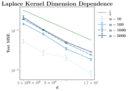
Figure 9: As $n$ grows, the excess MSE of Laplace KR trained on noisy data on $\mathcal{S}^{d}$ decays like $1/d$.

Appendix C Experimental Details

C.1 Datasets

Our experiments are performed using the following real and synthetic datasets:

• The $\mathbf{d}$-sphere: Data is sampled uniformly from $\mathcal{S}^{d}$ with noisy Gaussian targets. We use the convention that $d$ is the manifold dimension, and so $S^{d}$ is the hypersphere embedded in $\mathbb{R}^{d+1}$.

• MNIST. [LeCun, 1998, LeCun and Cortes, 2010]

• Binary MNIST. We binarize MNIST by classifying even vs. odd digits.

• CIFAR-10. [Krizhevsky et al., 2009]

• Binary CIFAR-10: We binarize CIFAR-10, forming two classes of animals (bird, cat, deer, dog) and vehicles (airplane, automobile, ship, truck).

• 0/1 SVHN. We binarize SVHN [Netzer et al., 2011], selecting the digits zero and one. We use the “train" and “extra" datasets for train data from the torchvision library.

• CINIC-10. [Darlow et al., 2018] 10-class image dataset with samples sourced from CIFAR-10 and Tiny ImageNet.

We obtained the MNIST, CIFAR-10, and SVHN datasets from the torchvision library.

In all experiments with subsampled train datasets, we uniformly sample over all training data available, and experimental results are averaged over multiple samples (and random seeds). All results are computed across the entire test set.

C.2 Experimental Setups

Unless otherwise stated, models are trained with no weight decay, dropout, or other regularization techniques, as is done in Zhang et al. [2017]. This encourages interpolation of training datasets even at high label noise levels. As is standard, we perform channel-wise normalization of image datasets.

During training of Binary CIFAR-10, we additionally employ random horizontal flips. On MNIST, CIFAR-10 and SVHN, we do not use flips or crops. As a result of this, and of our avoidance of regularization techniques, our models underperform current state-of-the-art methods, as is to be expected when intending to improve the state of understanding, not the state of the art.

We train the following models:

Kernel Regression: For synthetic data on $\mathcal{S}^{d}$ we directly solve the kernel regression problem by inverting the data kernel matrix. On MNIST, we create flattened vectors out of image data and train Gaussian and Laplacian kernels with stochastic gradient descent (SGD) in function space using EigenPro [Ma and Belkin, 2017]. EigenPro automatically computes an optimal batch size given the number of training data points and available memory on the GPU being used.

Neural Networks: We train multi-layer perceptrons (MLPs) and Wide ResNets (WRNs), and VGG networks [Simonyan and Zisserman, 2015] using SGD with batch size 128, initial learning rate of 0.1, and momentum of 0.9. For the MLPs on synthetic data and WRNs on SVHN we employ a learning rate decay factor of 0.1; for WRNs on CIFAR-10 we use a decay factor of 0.2. Per-experiment details on specific learning rate schedules are given in Appendix C.3.

Initial parameters for synthetic experiments are chosen by experimentation and largely guided by commonly used settings from non-synthetic cases. For WRNs, the learning rate decay factors, momentum, and batch size choices for CIFAR-10 and SVHN are chosen based on Zagoruyko and Komodakis [2016]. Wide ResNet model code is sourced from a publicly available Git repository. MLP model code and training/testing scripts are written in-house. Neural networks and EigenPro kernels are trained using PyTorch.

C.3 Experiment-Specific Details

MLP and Nearest Neighbor Noise Profiles on Binary MNIST (Figure 3)

We train $3\times 1024$ MLPs, 1-NN, and $k$-NN ($k\sim\log n$) models on Binary MNIST. Results are averaged over five independent runs with mean and standard error bars reported. Nearest Neighbor models use default settings from the scikit-learn library. MLPs are trained using Adam, a learning rate of $1\times 10^{-3}$, momentum of 0.9, batch size of 256. The learning rate is decayed by a factor of 0.1 at epochs 60 and 90. No learning rate warmup is used. All models are trained until the train loss reaches $1\times 10^{-4}$ and achieve 100% training accuracy.

Asymptotics of Kernel Regression on $d$-Sphere (Figure 4)

In this experiment, provided in Figure 4, we sample data, $\{x_{i}\}_{i}$, uniformly on $\mathcal{S}^{d}$ and train with pure noise target labels $y_{i}\sim\mathcal{N}(0,1)$. Test MSE is computed on clean labels, $y_{i}=0$. In experiments with a ridge, we use $\delta=0.1$. The kernel regression problem is solved by directly inverting the training data-data kernel matrix against the noisy labels. For this plot the lines represent the median of 100 independent runs and error regions are given for 25% and 75% quantiles.

Kernel Noise Profiles on MNIST (Figure 10)

Noise profiles for ridgeless Laplacian and Guassian kernels are provided for 10-class classification on MNIST. All models reach 100% training accuracy and $\leq 10^{-4}$ train MSE. Results are averaged over five independent runs.

MLP Noise Profiles on 10-Sphere (Figure 6(b))

In this experiment, we take $f^{*}(x)=1$ and inject label noise in the form of randomly flipping a fixed proportion, $p\in[0,0.5]$, of training labels to $-1$. The Bayes optimal classifier for $p<0.5$ is $\mu(x)=1$. The goal of this experiment is to show that even in the simplest case of learning a constant function, interpolating neural networks suffer from noisy training data. We present noise profiles for classification error as a function of training label flip probability in Figure 6(b).

The MLP is a $3\times 1024$ network trained using SGD with initial learning rate of 0.1, momentum of 0.9, and batch size of 128. For $n<120000$ we cut the learning rate by a factor of 0.1 at epoch 150 and again at epoch 350. For $n=120000,360000$ we cut the learning rate by a factor of 0.1 at epoch 500 and again at epoch 750.

In all experiments, the stopping criteria is a train MSE loss $\leq 1e^{-4}$, regardless of where the learning rate schedule has reached by that point. Controlling for train loss stopping point allows us to meaningfully compare models that have achieved the “same level of overfitting" and not introduce confounding factors due to late stage training effects. We average results over five independent runs.

WRN Noise Profiles on (Binary) CIFAR-10 and SVHN (Figures 2, 6(a), 7)

In all experiments, we train the Wide ResNet $28\times 10$ for 60 total epochs using SGD with initial learning rate of 0.1, momentum of 0.9, and batch size of 128. We cut the learning rate by a factor of 0.2 in CIFAR-10 experiments and 0.1 in SVHN experiments. The learning rate in both settings is cut once at epoch 30, and again at epoch 40.

Classification label noise is injected for each point $\{(x_{i},y_{i})\}_{i}$ by uniformly re-sampling labels from alternative class labels, excluding the ground truth label. We resample labels in this way for a fraction of the dataset, $p$. For 10 class and binary classification we vary $p\in[0.0,0.9]$ and $p\in[0.0,0.5]$, respectively. For example, $p=0.9$ indicates that we train with exactly $90\%$ label noise.

Test classification error is computed on the clean test set. For Binary CIFAR-10, CIFAR-10, and 0/1 SVHN we average results over three independent runs and report mean and standard error bars. On 0/1 SVHN, for each noise level and train set size, $n$, we perform 2-fold cross-validation to select the early-stop epoch which maximizes validation classification error averaged over both folds. We additionally do not consider the first ten epochs for early-stopping, during the learning rate warmup phase. We create the early-stopped noise profile from the classification test error attained at each of the early-stopped epoch choices.

MLP Error vs. Time (Figure 8)

We train a $4\times 512$ ReLU MLP trainsets of various sizes with $\{x_{i}\}$, sampled uniformly on $\mathcal{S}^{4}$. Training labels are given by $y_{i}=1+\mathcal{N}(0,1)$, a distribution for which the Bayes-optimal MSE is 1. To reduce statistical error, we compute test MSE with clean labels $y_{i}=1$ and simply add $1$ by hand to account for the noise. We average over five trials and plot against $t\equiv\text{[learning rate]}\times\text{[epoch number]}$. We train with full batch gradient descent using JAX and the neural-tangents library.

VGG Noise Profile on CINIC-10 (Figure 11)

We train a standard VGG-19 model with batch norm on the CINIC-10 dataset. We use SGD with initial learning rate 0.1 and momentum 0.9. We train for 200 epochs and decay the learning rate by a factor of 0.1 at epoch 60 and epoch 120.

C.4 Compute Details

Each neural network experiment and kernel experiment using EigenPro was run on a single NVIDIA V100 GPU. Experiments were performed in parallel using Expanse GPU nodes on XSEDE. [Towns et al., 2014] The final experiments for this paper took roughly 250 GPU-hours, and the experimentation phase of the project took roughly 1500 GPU-hours.

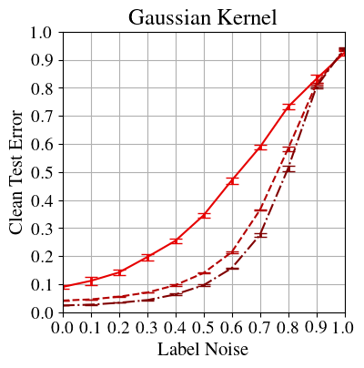
(a) Gaussian Kernel

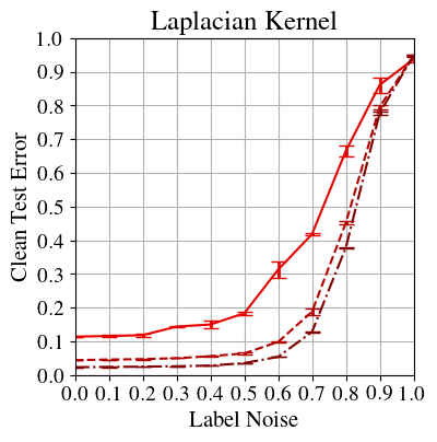
(b) Laplacian Kernel

Figure 10: We show noise profiles Gaussian and Laplacian kernels trained with label noise on 10-class MNIST for classification. We plot test classification error on the clean test set (no label noise) vs. training label noise. Overfitting is considered when the train MSE is $\leq 10^{-4}$. All models achieve 0 classification error on the training set.

Appendix D Additional Experimental Results

D.1 Kernel Noise Profiles on MNIST

We provide additional experimental results here for kernel noise profiles trained on MNIST data, as described in Appendix C.3.

In Figure 10 we show noise profiles for Gaussian and Laplacian kernels trained on MNIST data at varying values of training data size, $n$. We immediately see from the plots that the Laplacian kernel is more tempered than the Gaussian kernel.

Note that while the Gaussian kernel does not look catastrophic, the input dimension of MNIST is larger than all experiments on $\mathcal{S}^{d-1}$ shown in Figure 4. In this case, we would need a significantly larger number of training samples to observe the Gaussian kernel entering the catastrophic regime. Synthetic experiments on $\mathcal{S}^{1000}$ (not shown) up to 1 million training samples show that the Gaussian kernel still does not enter the catastrophic regime, therefore with MNIST only containing 60k samples we see a more tempered noise profile.

D.2 VGG Noise Profile

We additionally explore noise profiles for overfit VGG networks on the CINIC-10 dataset. We do so in order to show that both residual and non-residual convolutional networks, on differing image datasets, maintain a tempered noise profile. In Figure 11 we plot a 19-layer VGG network with batch norm overfit to the ten class CINIC-10 dataset.

On this dataset we were only able to run one experiment due to computational limitations, however in other experiments with deep neural networks we note low variance over the test error of DNNs at interpolation. Therefore, we expect the same to hold true over multiple runs of the VGG network on CINIC-10.

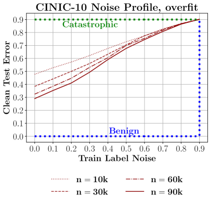
Figure 11: VGG-19 with batch norm overfit to the CINIC-10 dataset. We plot test classification error on the clean test set vs. training set label flip probability.

References

- Advani and Saxe [2017] Madhu S Advani and Andrew M Saxe. High-dimensional dynamics of generalization error in neural networks. arXiv preprint arXiv:1710.03667, 2017.
- Ali et al. [2019] Alnur Ali, J. Zico Kolter, and Ryan J. Tibshirani. A continuous-time view of early stopping for least squares regression. In Kamalika Chaudhuri and Masashi Sugiyama, editors, International Conference on Artificial Intelligence and Statistics, AISTATS 2019, volume 89 of Proceedings of Machine Learning Research, pages 1370–1378. PMLR, 2019.
- Bahri et al. [2020] Yasaman Bahri, Jonathan Kadmon, Jeffrey Pennington, Sam S Schoenholz, Jascha Sohl-Dickstein, and Surya Ganguli. Statistical mechanics of deep learning. Annual Review of Condensed Matter Physics, 11(1), 2020.
- Bahri et al. [2021] Yasaman Bahri, Ethan Dyer, Jared Kaplan, Jaehoon Lee, and Utkarsh Sharma. Explaining neural scaling laws. arXiv preprint arXiv:2102.06701, 2021.
- Bartlett et al. [2020] Peter L Bartlett, Philip M Long, Gábor Lugosi, and Alexander Tsigler. Benign overfitting in linear regression. Proceedings of the National Academy of Sciences, 2020.
- Bartlett et al. [2021] Peter L Bartlett, Andrea Montanari, and Alexander Rakhlin. Deep learning: a statistical viewpoint. arXiv preprint arXiv:2103.09177, 2021.
- Belkin et al. [2018a] Mikhail Belkin, Daniel J. Hsu, and Partha Mitra. Overfitting or perfect fitting? risk bounds for classification and regression rules that interpolate. In Samy Bengio, Hanna M. Wallach, Hugo Larochelle, Kristen Grauman, Nicolò Cesa-Bianchi, and Roman Garnett, editors, Advances in Neural Information Processing Systems 31: Annual Conference on Neural Information Processing Systems 2018, NeurIPS 2018, December 3-8, 2018, Montréal, Canada, pages 2306–2317, 2018a. URL https://proceedings.neurips.cc/paper/2018/hash/e22312179bf43e61576081a2f250f845-Abstract.html.
- Belkin et al. [2018b] Mikhail Belkin, Siyuan Ma, and Soumik Mandal. To understand deep learning we need to understand kernel learning. In Jennifer G. Dy and Andreas Krause, editors, Proceedings of the 35th International Conference on Machine Learning, ICML 2018, Stockholmsmässan, Stockholm, Sweden, July 10-15, 2018, volume 80 of Proceedings of Machine Learning Research, pages 540–548. PMLR, 2018b. URL http://proceedings.mlr.press/v80/belkin18a.html.
- Belkin et al. [2019a] Mikhail Belkin, Daniel Hsu, Siyuan Ma, and Soumik Mandal. Reconciling modern machine-learning practice and the classical bias–variance trade-off. Proceedings of the National Academy of Sciences, 116(32):15849–15854, 2019a.
- Belkin et al. [2019b] Mikhail Belkin, Daniel Hsu, and Ji Xu. Two models of double descent for weak features. arXiv preprint arXiv:1903.07571, 2019b.
- Belkin et al. [2019c] Mikhail Belkin, Alexander Rakhlin, and Alexandre B. Tsybakov. Does data interpolation contradict statistical optimality? In Kamalika Chaudhuri and Masashi Sugiyama, editors, The 22nd International Conference on Artificial Intelligence and Statistics, AISTATS 2019, 16-18 April 2019, Naha, Okinawa, Japan, volume 89 of Proceedings of Machine Learning Research, pages 1611–1619. PMLR, 2019c. URL http://proceedings.mlr.press/v89/belkin19a.html.
- Belkin et al. [2019d] Mikhail Belkin, Alexander Rakhlin, and Alexandre B Tsybakov. Does data interpolation contradict statistical optimality? In The 22nd International Conference on Artificial Intelligence and Statistics, pages 1611–1619. PMLR, 2019d.
- Bietti and Bach [2020] Alberto Bietti and Francis Bach. Deep equals shallow for relu networks in kernel regimes. arXiv preprint arXiv:2009.14397, 2020.
- Bordelon et al. [2020] Blake Bordelon, Abdulkadir Canatar, and Cengiz Pehlevan. Spectrum dependent learning curves in kernel regression and wide neural networks. In International Conference on Machine Learning, pages 1024–1034. PMLR, 2020.
- Canatar et al. [2021] Abdulkadir Canatar, Blake Bordelon, and Cengiz Pehlevan. Spectral bias and task-model alignment explain generalization in kernel regression and infinitely wide neural networks. Nature communications, 12(1):1–12, 2021.
- Cao et al. [2022] Yuan Cao, Zixiang Chen, Mikhail Belkin, and Quanquan Gu. Benign overfitting in two-layer convolutional neural networks. arXiv preprint arXiv:2202.06526, 2022.
- Chatterji and Long [2021] Niladri S Chatterji and Philip M Long. Foolish crowds support benign overfitting. arXiv preprint arXiv:2110.02914, 2021.
- Chatterji et al. [2021] Niladri S Chatterji, Philip M Long, and Peter L Bartlett. The interplay between implicit bias and benign overfitting in two-layer linear networks. arXiv preprint arXiv:2108.11489, 2021.
- Chaudhuri and Dasgupta [2014] Kamalika Chaudhuri and Sanjoy Dasgupta. Rates of convergence for nearest neighbor classification. Advances in Neural Information Processing Systems, 27, 2014.
- Chen and Xu [2020] Lin Chen and Sheng Xu. Deep neural tangent kernel and laplace kernel have the same rkhs. arXiv preprint arXiv:2009.10683, 2020.
- Christmann and Steinwart [2007] Andreas Christmann and Ingo Steinwart. Consistency and robustness of kernel-based regression in convex risk minimization. Bernoulli, 13(3):799–819, 2007.
- Cover and Hart [1967] Thomas Cover and Peter Hart. Nearest neighbor pattern classification. IEEE transactions on information theory, 13(1):21–27, 1967.
- Cui et al. [2021] Hugo Cui, Bruno Loureiro, Florent Krzakala, and Lenka Zdeborová. Generalization error rates in kernel regression: The crossover from the noiseless to noisy regime. Advances in Neural Information Processing Systems, 34:10131–10143, 2021.
- Darlow et al. [2018] Luke Nicholas Darlow, Elliot J. Crowley, Antreas Antoniou, and Amos J. Storkey. Cinic-10 is not imagenet or cifar-10. ArXiv, abs/1810.03505, 2018.
- d’Ascoli et al. [2020] Stéphane d’Ascoli, Levent Sagun, and Giulio Biroli. Triple descent and the two kinds of overfitting: Where & why do they appear? Advances in Neural Information Processing Systems, 33:3058–3069, 2020.
- Devroye et al. [1998] Luc Devroye, Laszlo Györfi, and Adam Krzyżak. The hilbert kernel regression estimate. Journal of Multivariate Analysis, 65(2):209–227, 1998.
- Frei et al. [2022] Spencer Frei, Niladri S Chatterji, and Peter L Bartlett. Benign overfitting without linearity: Neural network classifiers trained by gradient descent for noisy linear data. arXiv preprint arXiv:2202.05928, 2022.
- Geifman et al. [2020] Amnon Geifman, Abhay Yadav, Yoni Kasten, Meirav Galun, David Jacobs, and Basri Ronen. On the similarity between the laplace and neural tangent kernels. Advances in Neural Information Processing Systems, 33:1451–1461, 2020.
- Goldt et al. [2019] Sebastian Goldt, Madhu Advani, Andrew M Saxe, Florent Krzakala, and Lenka Zdeborová. Dynamics of stochastic gradient descent for two-layer neural networks in the teacher-student setup. Advances in neural information processing systems, 32, 2019.
- Hastie et al. [2019] Trevor Hastie, Andrea Montanari, Saharon Rosset, and Ryan J Tibshirani. Surprises in high-dimensional ridgeless least squares interpolation. arXiv preprint arXiv:1903.08560, 2019.
- Holzmüller [2021] David Holzmüller. On the universality of the double descent peak in ridgeless regression. In International Conference on Learning Representations, 2021. URL https://openreview.net/forum?id=0IO5VdnSAaH.
- Jacot et al. [2018] Arthur Jacot, Franck Gabriel, and Clément Hongler. Neural tangent kernel: Convergence and generalization in neural networks. Advances in neural information processing systems, 31, 2018.
- Jacot et al. [2020] Arthur Jacot, Berfin Şimşek, Francesco Spadaro, Clément Hongler, and Franck Gabriel. Kernel alignment risk estimator: risk prediction from training data. arXiv preprint arXiv:2006.09796, 2020.
- Ji et al. [2021] Ziwei Ji, Justin Li, and Matus Telgarsky. Early-stopped neural networks are consistent. Advances in Neural Information Processing Systems, 34, 2021.
- Koehler et al. [2021] Frederic Koehler, Lijia Zhou, Danica J Sutherland, and Nathan Srebro. Uniform convergence of interpolators: Gaussian width, norm bounds and benign overfitting. Advances in Neural Information Processing Systems, 34, 2021.
- Krizhevsky et al. [2009] Alex Krizhevsky et al. Learning multiple layers of features from tiny images. 2009.
- LeCun [1998] Yann LeCun. The mnist database of handwritten digits. http://yann. lecun. com/exdb/mnist/, 1998.
- LeCun and Cortes [2010] Yann LeCun and Corinna Cortes. MNIST handwritten digit database. 2010. URL http://yann.lecun.com/exdb/mnist/.
- Liang and Rakhlin [2018] Tengyuan Liang and Alexander Rakhlin. Just interpolate: Kernel" ridgeless" regression can generalize. arXiv preprint arXiv:1808.00387, 2018.
- Liang and Rakhlin [2020] Tengyuan Liang and Alexander Rakhlin. Just interpolate: Kernel “ridgeless” regression can generalize. The Annals of Statistics, 48(3):1329–1347, 2020.
- Ma and Belkin [2017] Siyuan Ma and Mikhail Belkin. Diving into the shallows: a computational perspective on large-scale shallow learning. Advances in neural information processing systems, 30, 2017.
- Mei and Montanari [2019] Song Mei and Andrea Montanari. The generalization error of random features regression: Precise asymptotics and double descent curve. arXiv preprint arXiv:1908.05355, 2019.
- Muthukumar et al. [2020] Vidya Muthukumar, Kailas Vodrahalli, Vignesh Subramanian, and Anant Sahai. Harmless interpolation of noisy data in regression. IEEE Journal on Selected Areas in Information Theory, 2020.
- Nakkiran and Bansal [2020] Preetum Nakkiran and Yamini Bansal. Distributional generalization: A new kind of generalization. arXiv preprint arXiv:2009.08092, 2020.
- Netzer et al. [2011] Yuval Netzer, Tao Wang, Adam Coates, Alessandro Bissacco, Bo Wu, and Andrew Y Ng. Reading digits in natural images with unsupervised feature learning. 2011.
- Neyshabur et al. [2015] Behnam Neyshabur, Ryota Tomioka, and Nathan Srebro. In search of the real inductive bias: On the role of implicit regularization in deep learning. In ICLR (Workshop), 2015.
- Radhakrishnan et al. [2022] Adityanarayanan Radhakrishnan, Mikhail Belkin, and Caroline Uhler. Wide and deep neural networks achieve optimality for classification, 2022. URL https://arxiv.org/abs/2204.14126.
- Rakhlin and Zhai [2019] Alexander Rakhlin and Xiyu Zhai. Consistency of interpolation with laplace kernels is a high-dimensional phenomenon. In Alina Beygelzimer and Daniel Hsu, editors, Conference on Learning Theory, COLT 2019, 25-28 June 2019, Phoenix, AZ, USA, volume 99 of Proceedings of Machine Learning Research, pages 2595–2623. PMLR, 2019. URL http://proceedings.mlr.press/v99/rakhlin19a.html.
- Simon et al. [2021] James B Simon, Madeline Dickens, Dhruva Karkada, and Michael R DeWeese. The eigenlearning framework: A conservation law perspective on kernel ridge regression and wide neural networks. arXiv preprint arXiv:2110.03922, 2021.
- Simon et al. [2022] James B. Simon, Sajant Anand, and Michael Robert DeWeese. Reverse engineering the neural tangent kernel. arXiv preprint arXiv:2106.03186, 2022.
- Simonyan and Zisserman [2015] Karen Simonyan and Andrew Zisserman. Very deep convolutional networks for large-scale image recognition. In Yoshua Bengio and Yann LeCun, editors, 3rd International Conference on Learning Representations, ICLR 2015, San Diego, CA, USA, May 7-9, 2015, Conference Track Proceedings, 2015. URL http://arxiv.org/abs/1409.1556.
- Spigler et al. [2020] Stefano Spigler, Mario Geiger, and Matthieu Wyart. Asymptotic learning curves of kernel methods: empirical data versus teacher–student paradigm. Journal of Statistical Mechanics: Theory and Experiment, 2020(12):124001, 2020.
- Towns et al. [2014] J. Towns, T. Cockerill, M. Dahan, I. Foster, K. Gaither, A. Grimshaw, V. Hazlewood, S. Lathrop, D. Lifka, G. D. Peterson, R. Roskies, J. Scott, and N. Wilkins-Diehr. Xsede: Accelerating scientific discovery. Computing in Science & Engineering, 16(05):62–74, sep 2014. ISSN 1558-366X. doi: 10.1109/MCSE.2014.80.
- Tsigler and Bartlett [2020] Alexander Tsigler and Peter L Bartlett. Benign overfitting in ridge regression. arXiv preprint arXiv:2009.14286, 2020.
- Zagoruyko and Komodakis [2016] Sergey Zagoruyko and Nikos Komodakis. Wide residual networks. In Richard C. Wilson, Edwin R. Hancock, and William A. P. Smith, editors, Proceedings of the British Machine Vision Conference 2016, BMVC 2016, York, UK, September 19-22, 2016. BMVA Press, 2016. URL http://www.bmva.org/bmvc/2016/papers/paper087/index.html.
- Zdeborová and Krzakala [2016] Lenka Zdeborová and Florent Krzakala. Statistical physics of inference: Thresholds and algorithms. Advances in Physics, 65(5):453–552, 2016.
- Zhang et al. [2017] Chiyuan Zhang, Samy Bengio, Moritz Hardt, Benjamin Recht, and Oriol Vinyals. Understanding deep learning requires rethinking generalization. In 5th International Conference on Learning Representations, ICLR 2017, Toulon, France, April 24-26, 2017, Conference Track Proceedings. OpenReview.net, 2017. URL https://openreview.net/forum?id=Sy8gdB9xx.
- Zhang et al. [2021] Chiyuan Zhang, Samy Bengio, Moritz Hardt, Benjamin Recht, and Oriol Vinyals. Understanding deep learning (still) requires rethinking generalization. Communications of the ACM, 64(3):107–115, 2021.