Self-Play PSRO: Toward Optimal Populations in Two-Player Zero-Sum Games

Abstract

In competitive two-agent environments, deep reinforcement learning (RL) methods based on the Double Oracle (DO) algorithm, such as Policy Space Response Oracles (PSRO) and Anytime PSRO (APSRO), iteratively add RL best response policies to a population. Eventually, an optimal mixture of these population policies will approximate a Nash equilibrium. However, these methods might need to add all deterministic policies before converging. In this work, we introduce Self-Play PSRO (SP-PSRO), a method that adds an approximately optimal stochastic policy to the population in each iteration. Instead of adding only deterministic best responses to the opponent’s least exploitable population mixture, SP-PSRO also learns an approximately optimal stochastic policy and adds it to the population as well. As a result, SP-PSRO empirically tends to converge much faster than APSRO and in many games converges in just a few iterations.

1 Introduction

In competitive two-agent environments, also known as zero-sum games, deep reinforcement learning (RL) methods based on the Double Oracle (DO) algorithm (McMahan et al., 2003), such as Policy Space Response Oracles (PSRO) (Lanctot et al., 2017) are some of the most promising methods for finding approximate Nash equilibria in large games. One reason is that they are simple to use with existing RL methods and naturally provide a measure of approximate exploitability, i.e. performance against the opponent’s best response. A second reason is that they effectively prune the game tree by only considering mixtures over policies that are already trained to be best responses. Finally, they can be used in games with large or continuous action spaces because they do not require full game-tree traversals. Methods based on PSRO such as AlphaStar (Vinyals et al., 2019) and Pipeline PSRO (McAleer et al., 2020) have achieved state-of-the-art performance on Starcraft and Stratego, respectively.

PSRO-based methods iteratively add RL best-response policies to a population. The best response for each player trains against a restricted distribution over the opponent’s existing population of policies. To find this restricted distribution, a Nash equilibrium (a pair of mutually best-responding policies) is computed in the restricted single-step game where each action correspond to choosing a policy from the population. Eventually, an optimal distribution over these population policies will approximate a Nash equilibrium in the full game.

Because PSRO adds pure-strategy (i.e. deterministic) best responses in each iteration, PSRO may need to add many policies to the population before they can support a Nash equilibrium. In fact, in certain games, all pure strategies will be added before finding a Nash equilibrium. This is because many games require mixing over a large number of pure strategies to arrive at a Nash equilibrium. Furthermore, before termination, the restricted distribution over population policies can be arbitrarily exploitable.

To address this second issue, APSRO (McAleer et al., 2022b) learns a restricted distribution that minimizes regret against the opponent’s best response policy while the latter is training. The resulting distribution approximates the least-exploitable restricted distribution over the population. However, since APSRO, like PSRO, adds pure best responses, it may also require a large population to converge.

In this work, we build on APSRO by aiming to add to the population in each iteration the myopically optimal policy, that is, the policy that maximally lowers the exploitability of the least-exploitable distribution of the resulting population. A key insight is that mixed strategies (i.e. stochastic policies) can lower the exploitability of a population more than pure strategies. To see this, note that a Nash equilibrium strategy is an optimal strategy to add, because the least-exploitable distribution over the resulting population will also be a Nash equilibrium strategy. If all Nash equilibria are mixed, as is often the case, then no pure strategy can be added to the population that reduces exploitability as much as the mixed strategy Nash equilibrium.

Although finding the optimal strategy to add is as hard as solving the original game, we find that adding a rough approximation to the optimal strategy can offer striking empirical benefits in quickly reducing the exploitability of the restricted distribution. We present Self-Play PSRO (SP-PSRO), which similarly to APSRO learns a restricted distribution over the population via no regret against the opponent’s best response. Additionally, SP-PSRO trains off-policy a new strategy against the opponent’s best response. At the end of each iteration, SP-PSRO add two strategies to the population: (1) the time-average of the new strategy and (2) the best response to the opponent’s restricted distribution. Section 4 clarifies this algorithm using formal notation.

By training the new strategy off-policy, SP-PSRO learns both with no additional experience. Experiments on normal form games and extensive-form games such as Liar’s Dice, Battleship, and Leduc Poker suggest that SP-PSRO can learn policies that are dramatically less exploitable than APSRO and PSRO.

2 Background

We consider extensive-form games with perfect recall (Hansen et al., 2004). An extensive-form game progresses through a sequence of player actions, and has a world state $w\in\mathcal{W}$ at each step. In an $N$-player game, $\mathcal{A}=\mathcal{A}_{1}\times\cdots\times\mathcal{A}_{N}$ is the space of joint actions for the players. $\mathcal{A}_{i}(w)\subseteq\mathcal{A}_{i}$ denotes the set of legal actions for player $i\in\mathcal{N}=\{1,\ldots,N\}$ at world state $w$ and $a=(a_{1},\ldots,a_{N})\in\mathcal{A}$ denotes a joint action. At each world state, after the players choose a joint action, a transition function $\mathcal{T}(w,a)\in\Delta^{\mathcal{W}}$ determines the probability distribution of the next world state $w^{\prime}$. Upon transition from world state $w$ to $w^{\prime}$ via joint action $a$, player $i$ makes an observation $o_{i}=\mathcal{O}_{i}(w,a,w^{\prime})$. In each world state $w$, player $i$ receives a reward $\mathcal{R}_{i}(w)$. The game ends when the players reach a terminal world state. In this paper, we consider games that are guaranteed to end in a finite number of actions.

A history is a sequence of actions and world states, denoted $h=(w^{0},a^{0},w^{1},a^{1},\ldots,w^{t})$, where $w^{0}$ is the known initial world state of the game. $\mathcal{R}_{i}(h)$ and $\mathcal{A}_{i}(h)$ are, respectively, the reward and set of legal actions for player $i$ in the last world state of a history $h$. An information set for player $i$, denoted by $s_{i}$, is a sequence of that player’s observations and actions up until that time $s_{i}(h)=(a_{i}^{0},o_{i}^{1},a_{i}^{1},\ldots,o_{i}^{t})$. Define the set of all information sets for player $i$ to be $\mathcal{I}_{i}$. The set of histories that correspond to an information set $s_{i}$ is denoted $\mathcal{H}(s_{i})=\{h:s_{i}(h)=s_{i}\}$, and it is assumed that they all share the same set of legal actions $\mathcal{A}_{i}(s_{i}(h))=\mathcal{A}_{i}(h)$.

A player’s strategy $\pi_{i}$ is a function mapping from an information set to a probability distribution over actions. A strategy profile $\pi$ is a tuple $(\pi_{1},\ldots,\pi_{N})$. All players other than $i$ are denoted $-i$, and their strategies are jointly denoted $\pi_{-i}$. A strategy for a history $h$ is denoted $\pi_{i}(h)=\pi_{i}(s_{i}(h))$ and $\pi(h)$ is the corresponding strategy profile. When a strategy $\pi_{i}$ is learned through RL, we refer to the learned strategy as a policy.

The expected value (EV) $v_{i}^{\pi}(h)$ for player $i$ is the expected sum of future rewards for player $i$ in history $h$, when all players play strategy profile $\pi$. The EV for an information set $s_{i}$ is denoted $v_{i}^{\pi}(s_{i})$ and the EV for the entire game is denoted $v_{i}(\pi)$. A two-player zero-sum game has $v_{1}(\pi)+v_{2}(\pi)=0$ for all strategy profiles $\pi$. The EV for an action in an information set is denoted $v_{i}^{\pi}(s_{i},a_{i})$. A Nash equilibrium (NE) is a strategy profile such that, if all players played their NE strategy, no player could achieve higher EV by deviating from it. Formally, $\pi^{*}$ is a NE if $v_{i}(\pi^{*})=\max_{\pi_{i}}v_{i}(\pi_{i},\pi^{*}_{-i})$ for each player $i$.

The exploitability $e(\pi)$ of a strategy profile $\pi$ is defined as $e(\pi)=\sum_{i\in\mathcal{N}}\max_{\pi^{\prime}_{i}}v_{i}(\pi^{\prime}_{i},\pi_{-i})$. A best response (BR) strategy $\mathbb{BR}_{i}(\pi_{-i})$ for player $i$ to a strategy $\pi_{-i}$ is a strategy that maximally exploits $\pi_{-i}$: $\mathbb{BR}_{i}(\pi_{-i})=\arg\max_{\pi_{i}}v_{i}(\pi_{i},\pi_{-i})$. An $\bm{\epsilon}$-best response ($\bm{\epsilon}$-BR) strategy $\mathbb{BR}^{\epsilon}_{i}(\pi_{-i})$ for player $i$ to a strategy $\pi_{-i}$ is a strategy that is at most $\epsilon$ worse for player $i$ than the best response: $v_{i}(\mathbb{BR}^{\epsilon}_{i}(\pi_{-i}),\pi_{-i})\geq v_{i}(\mathbb{BR}_{i}(\pi_{-i}),\pi_{-i})-\epsilon$. An $\bm{\epsilon}$-Nash equilibrium ($\bm{\epsilon}$-NE) is a strategy profile $\pi$ in which, for each player $i$, $\pi_{i}$ is an $\epsilon$-BR to $\pi_{-i}$.

A normal-form game is a single-step extensive-form game. An extensive-form game induces a normal-form game in which the legal actions for player $i$ are its deterministic strategies $\operatorname*{\vartimes}_{s_{i}\in\mathcal{I}_{i}}\mathcal{A}_{i}(s_{i})$. These deterministic strategies are called pure strategies of the normal-form game. A mixed strategy is a distribution over a player’s pure strategies.

3 Related Work

Many recent works study the intersection of reinforcement learning and game theory. QPG (Srinivasan et al., 2018) is an algorithm based on policy gradient that empirically converges to a NE when the learning rate is annealed. NeuRD (Hennes et al., 2020), Magnetic Mirror Descent (Sokota et al., 2022), and F-FoReL (Perolat et al., 2021) approximate replicator dynamics, mirror descent, and follow the regularized leader, respectively, with policy gradients. DeepNash, which is based on F-FoReL and NeuRD has achieved expert level performance at Stratego (Perolat et al., 2022). Markov games generalize MDPs where players take simultaneous actions and observe the ground state of the game. Recent literature has shown that reinforcement learning algorithms converge to Nash equilibrium in two-player zero-sum Markov games (Brafman & Tennenholtz, 2002; Wei et al., 2017; Perolat et al., 2018; Xie et al., 2020; Daskalakis et al., 2020; Jin et al., 2021) and in multi-player general-sum Markov potential games (Leonardos et al., 2021; Mguni et al., 2021; Fox et al., 2022; Zhang et al., 2021; Ding et al., 2022). Deep methods based on CFR (McAleer et al., 2022a; Steinberger et al., 2020; Brown et al., 2019) are another promising direction for scaling to large games. In this work we focus on a different set of deep RL algorithms for games based on PSRO. Advances made to PSRO can potentially be combined with the above methods via XDO (McAleer et al., 2021).

3.1 Double Oracle (DO) and Policy Space Response Oracles (PSRO)

Double Oracle (McMahan et al., 2003) is an algorithm for finding a Nash equilibrium (NE) in normal-form games. The algorithm works by keeping a population of strategies $\Pi^{t}$ at time $t$. In each iteration, a NE $\pi^{*,t}$ is computed for the game restricted to strategies in $\Pi^{t}$. Then, a best response to this restricted NE for each player $\mathbb{BR}_{i}(\pi^{*,t}_{-i})$ is computed and added to the population $\Pi_{i}^{t+1}=\Pi_{i}^{t}\cup\{\mathbb{BR}_{i}(\pi^{*,t}_{-i})\}$ for $i\in\{1,2\}$. Although in the worst case DO must add all pure strategies, in many games DO empirically terminates early and outperforms alternative approaches.

Algorithm 1 Policy Space Response Oracle (PSRO) Lanctot et al. (2017)

  Result: Nash Equilibrium

  Input: Initial population $\Pi^{0}$

  repeat {for $t=0,1,\ldots$}

     $\pi^{r}\leftarrow$ NE in game restricted to strategies in $\Pi^{t}$

     for $i\in\{1,2\}$ do

        for $m$ iterations do

           Update policy $\beta_{-i}$ toward $\mathbb{BR}_{-i}(\pi^{r}_{i})$

     $\Pi^{t+1}_{i}\leftarrow\Pi^{t}_{i}\cup\{\beta_{i}\}$ for $i\in\{1,2\}$

  until No novel best response exists for either player

  Return: $\pi^{r}$

Policy-Space Response Oracles (PSRO) Lanctot et al. (2017) scales DO to large games by using reinforcement learning to approximate a best response. The restricted-game NE is computed on the empirical game matrix $U^{\Pi}$, generated by having each policy in the population $\Pi$ play each opponent policy and tracking average utility in a $\Pi_{1}\times\Pi_{2}$ payoff matrix (Wellman, 2006). PSRO is described in Algorithm 1.

Several methods related to PSRO have been published in recent years. AlphaStar (Vinyals et al., 2019) trains a population of policies through a procedure that is somewhat similar to PSRO. AlphaStar also uses some elements of self-play when constructing its population, and outputs a population-restricted NE at test time. NXDO (McAleer et al., 2021) iteratively adds reinforcement learning policies to a population but solves an extensive-form restricted game, which has been shown to be more efficient than solving a matrix-form restricted game as in PSRO. P2SRO (McAleer et al., 2020) parallelizes PSRO with convergence guarantees. Other work has looked at incorporating diversity (Liu et al., 2021; Perez-Nieves et al., 2021) in the best response objective. However, since the best response is still pure, these methods suffer from the same problems of PSRO and APSRO as previously described. Other methods generalize PSRO to more players (Muller et al., 2020; Marris et al., 2021), and meta-learn the restricted-NE population distribution (Feng et al., 2021). Slumbers et al. (2022) propose a PSRO-like approach for learning risk-averse equilibria.

3.2 Anytime-PSRO (APSRO)

Algorithm 2 Anytime PSRO (APSRO) (McAleer et al., 2022b)

  Result: Approximate Nash Equilibrium

  Input: Initial population $\Pi^{0}$

  while Not Terminated {$t=0,1,\ldots$} do

     Initialize $\pi^{r}_{i}$ to uniform over $\Pi^{t}_{i}$ for $i\in\{1,2\}$ 

     for $i\in\{1,2\}$ do

        for $n$ iterations do

           for $m$ iterations do

              Update policy $\beta_{-i}$ toward $\mathbb{BR}_{-i}(\pi^{r}_{i})$

           Update $\pi^{r}_{i}$ via regret minimization vs. $\beta_{-i}$ 

     $\Pi^{t+1}_{i}=\Pi^{t}_{i}\cup\{\beta_{i}\}$ for $i\in\{1,2\}$ 

  Return: $\pi^{r}$

Although PSRO is guaranteed to converge to a NE by, at worst, enumerating all pure strategies, before convergence the exploitability of the restricted NE distribution may increase arbitrarily. This becomes a problem in large games where full enumeration is infeasible due to the large number of pure strategies. Anytime PSRO (APSRO) (McAleer et al., 2022b) is a PSRO-type algorithm that is guaranteed, up to approximation error, to not increase exploitability from one iteration to the next.

In each iteration, APSRO creates for each player a different restricted game than PSRO does. The restricted game $G^{i}(\Pi)$ for player $i$ is created by restricting that player to only play strategies included in their population $\Pi_{i}$, while the opponent can play any strategy in the full game. The game value of $G^{i}(\Pi)$ for player $i$ is

$$\max_{\pi_{i}\in\Pi_{i}}\min_{\pi_{-i}}v_{i}(\pi_{i},\pi_{-i}).$$ (1)

The restricted game $G^{i}(\Pi)$ for player $i$ is then approximately solved by learning a restricted distribution $\pi_{i}^{r}$ over the population policies $\Pi_{i}$ via a no-regret algorithm against the opponent’s best response $\beta_{-i}$, at the same time that the latter is trained with reinforcement learning. A description of APSRO is given in algorithm 2.

4 Self-Play PSRO

Although APSRO does not increase exploitability from one iteration to the next by adding to each player’s population the pure-strategy best response $\beta_{i}$ to the opponent’s restricted distribution $\pi^{r}_{-i}$, it is not guaranteed to decrease exploitability. $\beta_{i}$ may not be the myopically optimal pure strategy whose addition to $\Pi_{i}$ decreases exploitability the most. Moreover, adding mixed strategies can generally be better than adding pure strategies.

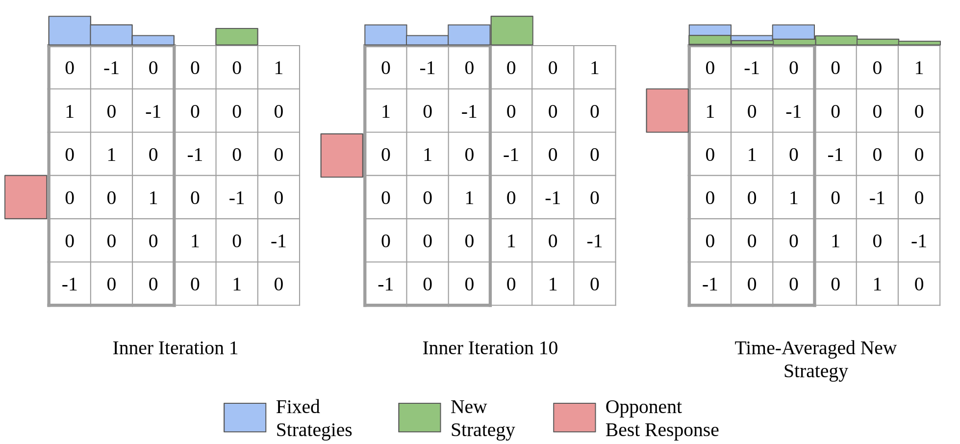
Figure 1: SP-PSRO. In this diagram we show how SP-PSRO works within an iteration from the perspective of the column player. The fixed population is shown in blue and the new strategy is shown in green. Every inner iteration, three things happen. (1) The opponent best response updates toward a best response to the current distribution over both the fixed population and the new strategy. (2) The new strategy updates toward a best response against the opponent best response. (3) The restricted distribution updates via no regret against the opponent best response. In the final iteration, the time-average of the new strategy and the player’s best response to the opponent’s restricted distribution (which is trained in a symmetric manner) are added to the population and the cycle starts again.

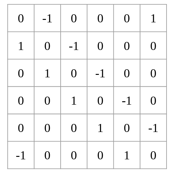
Figure 2: Big RPS Game. Any algorithm that only adds pure best responses, such as PSRO or APSRO, will expand all pure strategies before converging.

For example, consider the generalized Rock–Paper–Scissors game shown in Figure 2. In this game, the NE mixes equally over all pure strategies. As a result, any DO method that only adds pure strategies will have to enumerate all pure strategies in the game before supporting the NE.

Ideally, we would like to add a mixed strategy that decreases exploitability the most. A single-iteration objective would then be to find the strategy such that after it is added to the population and the least-exploitable distribution is computed over this new population, the exploitability of the resulting distribution is the lowest. In this example game, a mixed strategy that mixes over the pure strategies equally is optimal and will lower exploitability more than any pure strategy. The following proposition makes this point more explicit.

Although the Nash equilibrium of the original game is the optimal mixed strategy to add to the population, finding a Nash equilibrium of the original game is very expensive and is our main goal in the first place. However, even if the mixed strategy we add is not a Nash equilibrium strategy, the fact that it is a mixed strategy instead of a pure strategy empirically decreases exploitability faster in early iterations than pure strategies.

But we can potentially do better than just adding a random mixed strategy. By trying to roughly approximate a Nash equilibrium of the original game, we can expect to improve our population exploitability more than random. In other words, the closer the new strategy is to being a Nash equilibrium of the original game, the more it will lower the resulting exploitability of the population.

Motivated by this, we propose Self-Play PSRO, a PSRO method that learns a new mixed strategy by best-responding to the opponent best response via off-policy reinforcement learning. To heuristically better approximate a Nash equilibrium, after the iteration has finished we output the time-average of the new strategy during self play.

Algorithm 3 Self-Play PSRO

  Result: Approximate Nash Equilibrium

  Input: Initial population $\Pi^{0}\cup\{\nu_{i}\}$

  while Not Terminated {$t=0,1,\ldots$} do

     Initialize new strategy $\nu_{i}$ arbitrarily 

     Initialize $\pi^{r}_{i}$ to uniform over $\Pi^{t}_{i}\cup\{\nu_{i}\}$ for $i\in\{1,2\}$ 

     for $i\in\{1,2\}$ do

        for $n$ iterations do

           for $m$ iterations do

              Update policy $\beta_{-i}$ toward $\mathbb{BR}_{-i}(\pi^{r}_{i})$

              Update new strategy $\nu_{i}$ toward $\mathbb{BR}_{i}(\beta_{-i})$

           Update $\pi^{r}_{i}$ via regret minimization vs. $\beta_{-i}$ 

     $\Pi^{t+1}_{i}=\Pi^{t}_{i}\cup\{\beta_{i},\bar{\nu}_{i}\}$ for $i\in\{1,2\}$ 

  Return: $\pi^{r}$

SP-PSRO works by maintaining a restricted distribution $\pi_{i}^{r}$ over a population. Unlike PSRO, where $\pi_{i}^{r}$ is the NE of the restricted game, SP-PSRO trains $\pi_{i}^{r}$ as in APSRO, via regret minimization. In addition, at the beginning of each iteration, a new strategy $\nu_{i}$ is initialized and added to the population.

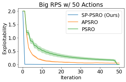
(a) Big RPS with 50 Actions

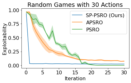
(b) Random Games with 30 Actions

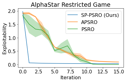
(c) AlphaStar Restricted Game

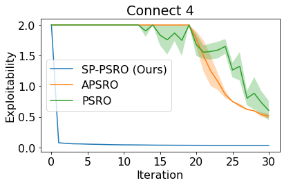
(d) Connect 4 Restricted Game

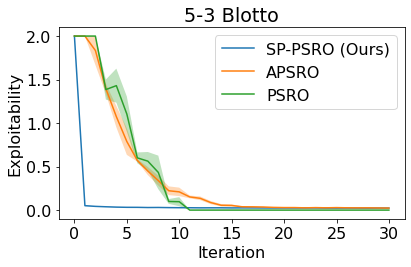
(e) 5-3 Blotto

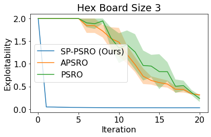
(f) Hex-3 Restricted Game

Figure 3: Normal-form games

During an iteration, three training processes unfold concurrently. First, as in APSRO, the opponent’s best response $\beta_{i}$ takes multiple update steps toward a best response to the current restricted distribution $\mathbb{BR}_{-i}(\pi^{r}_{i})$. Second, the new strategy $\nu_{i}$ is updated toward a best response to the opponent best response $\mathbb{BR}_{i}(\beta_{-i})$. Third, the restricted distribution $\pi_{i}^{r}$ is trained via regret minimization; this includes updating the probability of the new population strategy $\nu_{i}$, even as $\nu_{i}$ is also trained. This procedure can be thought of a form of self-play, in which the new strategy is updating against the opponent best response, while the opponent best response is updating against the restricted distribution, which also contains the new strategy. When the episode is terminated, the time-average $\bar{\nu_{i}}$ of $\nu_{i}$ is added to the population. Averaging over the updates of $\nu_{i}$ can be accomplished by checkpointing the policy over time and uniformly sampling checkpoints, or by training a neural network to distill a buffer of experience generated by $\nu_{i}$ as it trains. Since the new strategy is trained via off-policy reinforcement learning, SP-PSRO uses the exact same amount of environment experience as APSRO, but does require more compute to train the new network.

5 Experiments

5.1 Normal Form Experiments

In this section we describe experiments on normal form games. To emulate the process of a strategy $\pi$ learning a best response to another policy $\pi^{\prime}$, in every inner loop iteration $t$ we update $\pi$ by the following learning rule: $\pi_{t+1}=(1-\lambda)\pi_{t}+\lambda\times\mathbb{BR}_{i}(\pi^{\prime})$. We consider six normal form games. The first, described in Figure 2, is a large generalized Rock–Paper–Scissors game. The second is a random normal-form games generated by sampling each entry in the payoff matrix independently from a standard uniform distribution. The third game is the final restricted game of the AlphaStar population (Vinyals et al., 2019). The next three are taken from Perez-Nieves et al. (2021) and include a connect 4 restricted game, 5-3 blotto, a Hex restricted game.

5.2 Tabular Experiments

We evaluated SP-PSRO with tabular methods in a variety of games. We applied tabular SP-PSRO to the domains of Leduc Poker (9,457 states), a tiny version of Battleship (1,573 states), repeated Rock Paper Scissors (9,841 states), and a small version of Goofspiel (18,426 states). The experiments used game implementations and tools from the OpenSpiel library (Lanctot et al., 2019).

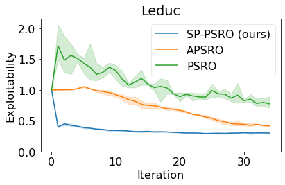
(a) Leduc Poker

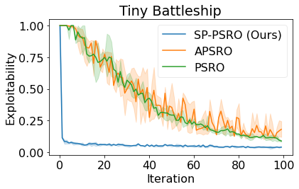
(b) Battleship

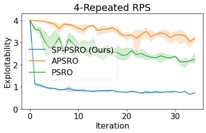
(c) Repeated RPS

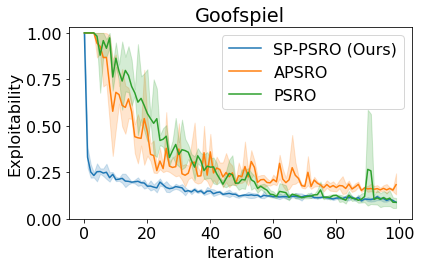
(d) Goofspiel

Figure 4: Extensive-form games with tabular Q-learning best responses

5.2.1 Results

SP-PSRO outperforms APSRO and PSRO in Leduc Poker (Figure 4(a)). We see a drastic improvement in performance starting in the first iteration. The hyperparameters for APSRO are the same as given in McAleer et al. (2022b). SP-PSRO outperforms both APSRO and PSRO in the small Battleship game (Figure 4(b)), 4-repeated Rock Paper Scissors (Figure 4(c)), and the small Goofspiel game (Figure 4(d)). In these 3 games, we use the same amount of compute for APSRO and SP-PSRO.

5.2.2 Tabular Experiment Details

In these experiments, the new population strategy $\nu_{i}$ and the BR $\beta_{-i}$ are the policies of tabular Q-learning agents. The tabular Q-learning agents are $\epsilon$-greedy. When training the Q-learning agent for $\beta_{-i}$, the episodes are also used to train the agent for $\nu_{i}$, in an off-policy manner. We use a constant value of $\epsilon$ for both agents. Note that this means that each agent learns to best-respond to the $\epsilon$-greedy agent of the other, instead of the underlying policy of the other. However, this approach uses half as many training episodes as would be needed if each trained independently, and still performs well.

5.3 Deep Reinforcement Learning Experiments

When using deep reinforcement learning best-response operators with DDQN Van Hasselt et al. (2016), SP-PSRO outperforms APSRO and PSRO in terms of sample efficiency (Figure 5). Tested on Liar’s Dice, a small version of Battleship, and 4x Repeated RPS, SP-PSRO sees a significant improvement against other baselines in early-iteration exploitability. This early exploitability advantage seen by SP-PSRO is especially present in repeated RPS (Figure 5(c)), where the relative performance seen with deep RL methods roughly matches that of tabular methods.

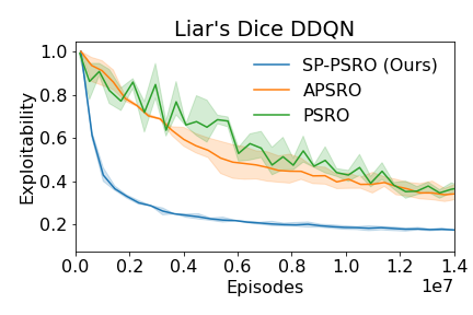
(a) DRL Liars Dice

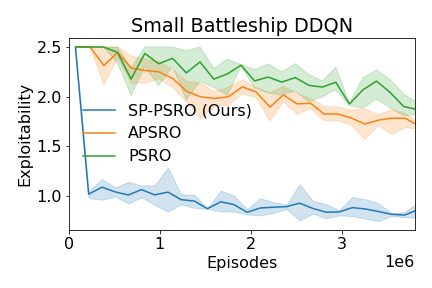
(b) DRL Battleship

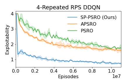
(c) DRL Repeated RPS

Figure 5: Extensive-form games with DDQN best responses

6 Discussion

6.1 Limitations

One limitation of SP-PSRO is that if the new strategies happen to not be useful, including the new strategy can hurt the performance of the restricted distribution. This is primarily because it is harder to learn a no-regret distribution when one of the arms is changing, and secondly because including more actions (strategies) makes it harder for the no regret algorithm as well. A related limitation of SP-PSRO is that because including the new strategy makes it harder to learn the restricted distribution, we find that SP-PSRO tends to plateau higher than APSRO and can even slightly increase exploitability. To mitigate this, we switch over to APSRO after some iterations, but we have not introduced a principled method of determining when is a good time to switch. A third limitation of our method is that extra compute needs to be used to train the new strategy $\nu$. Also, if the average strategy is computed via supervised learning on a replay buffer of experience, this adds additional compute requirements to the algorithm. Lastly, SP-PSRO is somewhat unprincipled in that the new strategy generated by the self-play procedure is not guaranteed to be close to a Nash equilibrium, even in the time average. In the following section we speculate on interesting research directions to improve this part of SP-PSRO.

6.2 Future Work

SP-PSRO opens up exciting connections to the literature regarding learning approximate Nash equilibria in large games. In particular, although we introduce an unprincipled self play method for approximating a Nash equilibrium, future work can find better ways of creating a new strategy that will better approximate a Nash equilibrium and therefore result in lower exploitability every iteration. For example, the data collected via the the opponent best response training against the restricted distribution can be used in a Monte-Carlo CFR-type algorithm to minimize regret on information sets visited during training.

These directions open up the possibility of deriving the first regret bounds for double oracle algorithms that do not rely on the size of the effective pure strategy set (Dinh et al., 2021). It also introduces the possibility of combining the deep reinforcement learning from the best response with methods based on deep CFR. For example, perhaps the Q networks learned from the best responses can be used to minimize regret for the new strategy.

Finally, our algorithm is a normal-form algorithm in that it mixes at the root of the game tree. McAleer et al. (2021) showed that this can be exponentially bad in the worst case, and introduced tabular (XDO) and deep (NXDO) algorithms to fix this problem. An interesting future direction is combining SP-PSRO with XDO and NXDO.

Appendix A Additional Normal-Form Experiments

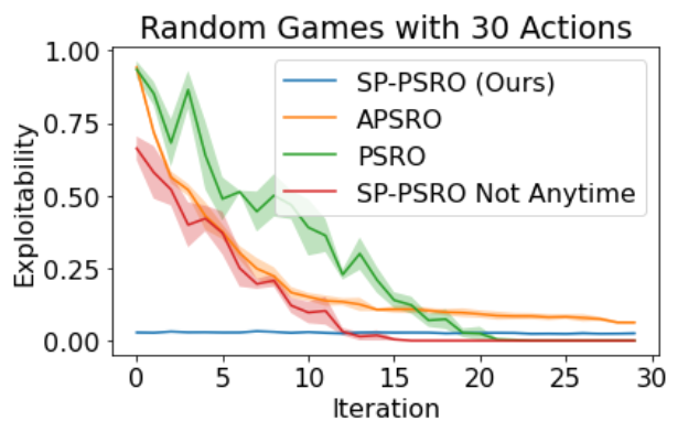
(a) Random Games with 30 Actions

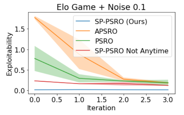
(b) Elo Game + Noise 0.1

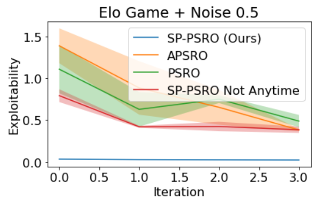
(c) Elo Game + Noise 0.5

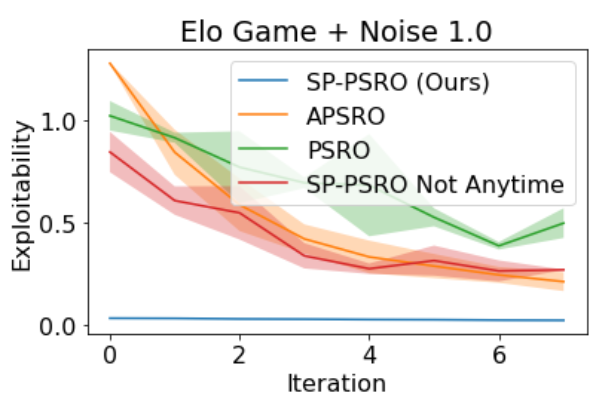
(d) Elo Game + Noise 1.0

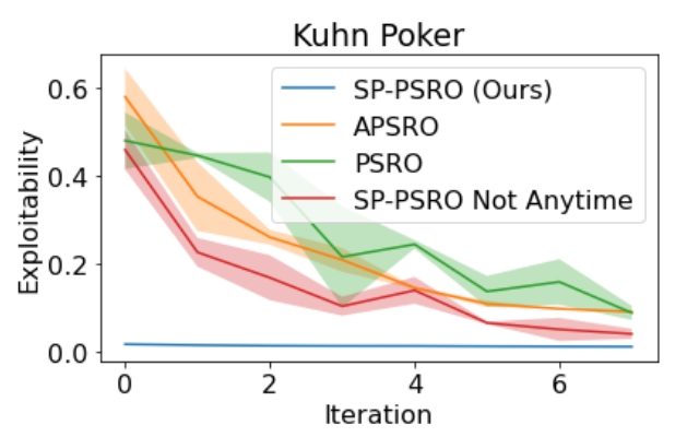
(e) Kuhn Poker

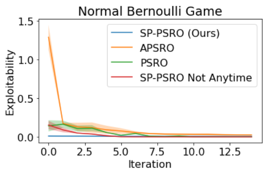
(f) Normal Bernoulli Game

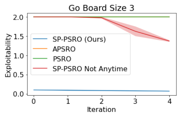
(g) Go Board Size 3

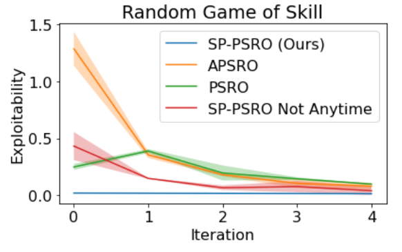
(h) Random Game of Skill

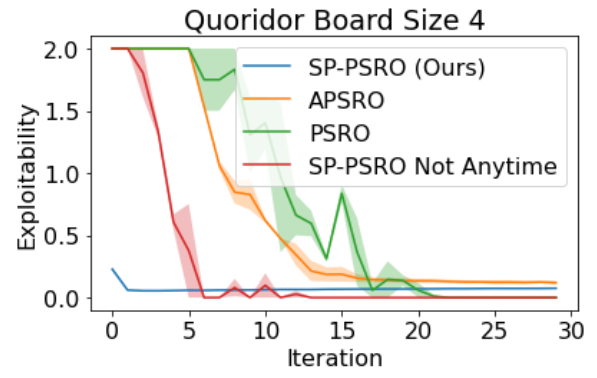
(i) Quoridor Board Size 4

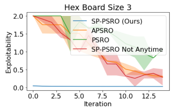
(j) Hex Board Size 3

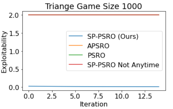
(k) Triangle Game Size 1000

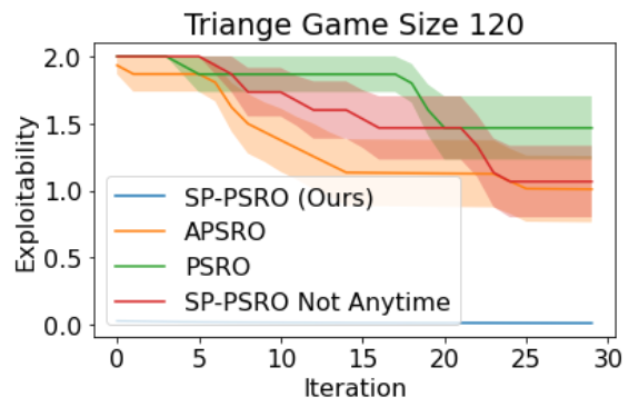
(l) Triangle Game Size 120

Figure 6: Additional Normal-Form Game Experiments

In this section we report additional normal form game experiments. All games in this section are from Perez-Nieves et al. (2021). Note that the zeroth iteration is not included in the plots. Similar to the main results in the paper we find that SP-PSRO achieves much lower exploitability than existing PSRO based methods and does so much faster, across all games studied. We include an ablation, labeled SP-PSRO Not Anytime, that is the same as SP-PSRO in that it trains a new strategy to be a best response to the opponent best response, but unlike SP-PSRO does not update the restricted distribution via no-regret as in Anytime PSRO. As shown in the figures, Anytime PSRO is a crucial piece of SP-PSRO, and excluding this aspect results in much worse performance. We find that when Anytime PSRO is excluded, the opponent best response will be best responding to a static opponent, and the best response to this best response will tend to be a pure strategy. As a result, we do not get to explore the strategy space, and the average new strategy will simply be another pure strategy. In some games we see that SP-PSRO Not Anytime and PSRO converge to lower exploitability than SP-PSRO and Anytime PSRO. This is because SP-PSRO Not Anytime and PSRO both use exact meta-solvers, which return the exact Nash equilibrium upon convergence, while SP-PSRO and APSRO use a no-regret procedure to find the least-exploitable restricted distribution.

Appendix B Additional Neural Experiments

We compare an alternate last-iterate version of SP-PSRO against the default SP-PSRO method and other baselines in Figure 7. In the SP-PSRO last-iterate variant, we add the pure-strategy weights of $\nu_{i}$ in its final RL iteration to the population rather than calculating and adding the time average $\bar{\nu_{i}}$. Exploitability is also calculated using $\nu_{i}$ rather than $\bar{\nu_{i}}$. SP-PSRO last-iterate improves upon APSRO and PSRO due to the additional, potentially useful, population policy. However, $\nu_{i}$ is less able to roughly approximate a NE because it represents a single pure-strategy approximate best-response to $\beta_{-i}$ rather than a mixture of multiple best-responses. Because of this, we still see an additional gain in exploitability versus sample-efficiency when transitioning from SP-PSRO last-iterate to the default time-average version of SP-PSRO.

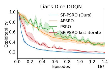
(a) DRL Liars Dice

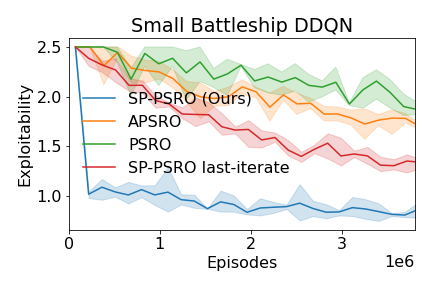
(b) DRL Battleship

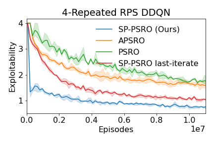
(c) DRL Repeated RPS

Figure 7: SP-PSRO last-iterate on extensive-form games with DDQN best responses

Appendix C Extensive-Form Game Environments

All extensive-form games tested with are from the OpenSpiel framework (Lanctot et al., 2019), and can be loaded using OpenSpiel with the following parameters:

Leduc

Game Name: leduc_poker
Parameters: {"players": 2}

Goofspiel

Game Name: goofspiel
Parameters: {"imp_info": True, "num_cards": 5,
"points_order":"descending",}

Tiny Battleship

Game Name: battleship
Parameters: {"board_width": 2, "board_height": 2,
"ship_sizes": ’[1]’, "ship_values": ’[1]’,
"num_shots": 2, "allow_repeated_shots": False,}

Small Battleship

Game Name: battleship
Parameters: {"board_width": 2, "board_height": 2,
"ship_sizes": "[1;2]", "ship_values": "[1;2]",
"num_shots": 4, "allow_repeated_shots": False}

4x Repeated RPS

Game Name: repeated_game
Parameters: {"num_repetitions": 4, "enable_infostate": True,
"stage_game": "matrix_rps"}

Liar’s Dice

Game Name: liars_dice
Parameters: None

Goofspiel and Repeated RPS are converted from simultaneous-move games into turn-based games using OpenSpiel’s convert_to_turn_based() game transform. Repeated RPS is created from the matrix_rps game using the create_repeated_game game transform.

Appendix D Tabular Training Details

In all tabular experiments, when calculating the payoff for a strategy profile ($v_{i}(\pi)$), the payoff is calculated exactly using a full tree traversal.

D.1 SP-PSRO

We performed a hyperparameter sweep to find the number of episodes per iteration and number of Exp3 updates per iteration which minimize exploitability in Leduc poker after 35 iterations of SP-PSRO (Table 1). We used these hyperparameters for SP-PSRO for tabular experiments in all games.

In each iteration, we split the Q-learning training and Exp3 updates into 600 equally-sized batches each, and alternate between a batch of Exp3 updates and a batch of Q-learning episodes until the end of the iteration. For example, when using $799,800$ episodes and $19,800$ Exp3 updates per iteration, we repeat the following 600 times: for each player, perform $799,800/600=1333$ Q-learning episodes and then $19,800/600=33$ Exp3 updates.

episodes per iteration	799,800
Exp3 updates per iteration	19,800
Q-learning learning rate	0.025
Q-learning exploration $\epsilon$	Constant, 0.2

Table 1: Tabular experiment details

For each Q-learning episode: we sample one policy $\pi_{i}$ for player $i$ from the distribution $\pi^{r}_{i}$, and then the sampled policy $\pi_{i}$ and the opponent Q-learning agent for $\beta_{-i}$ play an episode against each other. If the sampled policy $\pi_{i}$ corresponds to the new strategy $\nu_{i}$, it plays with $\epsilon$-greedy exploration. The opponent Q-learning agent always plays with $\epsilon$-greedy exploration. The episode is used to update the Q-learning agent for $\beta_{-i}$. The episode is also used to update the Q-learning agent for $\nu_{i}$, regardless of whether or not the chosen $\pi_{i}$ is $\nu_{i}$.

D.2 APSRO

Tabular APSRO experiments were performed according to McAleer et al. (2022b). We use the same code as for SP-PSRO, with the difference being that we do not create a new policy $\nu_{i}$.

D.3 PSRO

For tabular PSRO experiments: in each iteration, we first compute the empirical game payoff matrix, then use linear programming to find the Nash of the empirical game. We train Q-learning agents for each player against the other’s empirical game Nash, and then add these to the population. The Q-learning agents use the same hyperparameters as for SP-PSRO and A-PSRO.

Appendix E Neural Training Details

E.1 PSRO

For neural experiments, the PSRO empirical payoff matrix is estimated using 3000 evaluation rollouts per policy matchup, and the meta-game NE is calculated using 2000 iterations of Fictitious Play (Brown, 1951). APSRO and SP-PSRO skip calculating the empirical payoff matrix. We do not count experience used to generate payoff matrix utilities in comparisons with PSRO.

E.2 APSRO

We use the same neural APSRO method as provided by McAleer et al. (2022b), using the Multiplicative Weights Update (MWU) algorithm as the no-regret metasolver with a learning rate of 0.1 and updating every 10th RL iteration. Action payoffs for MWU corresponding to expected utilities for population policies in $\Pi_{i}^{t}$ against the current $\beta_{-i}$ are estimated by averaging the empirical payoffs from the last 1000 rollouts in which each population policy was sampled. Exploitability is measured against the time-average of the MWU mixed-strategy from each APSRO iteration.

E.3 SP-PSRO

For SP-PSRO, we use the same MWU no-regret solver and parameters as we do with APSRO, where the actively-learning new strategy $\nu_{i}$ is included as an action for the no-regret solver. Because $\nu_{i}$ would by default only collect experience when the no-regret solver samples it, we additionally provide $\nu_{i}$ with off-policy experience from all other policies in the population $\Pi_{i}^{t}$ when they are sampled and generate experience as well.

We train the time-average $\bar{\nu_{i}}$ of $\nu_{i}$ as a neural network, and to do so, we save all experience generated by $\nu_{i}$ to a buffer using reservoir sampling (Vitter, 1985; Heinrich & Silver, 2016) with a maximum capacity of 2e6 samples. After BR training is complete, we use supervised learning to train a softmax policy on the reservoir buffer data with cross-entropy loss on actions given observations to distill the time-average of the new policy $\nu_{i}$. To ensure that enough experience from $\nu_{i}$ is always generated and added to the reservoir buffer, a small fixed portion $p$ of all experience rollouts in the BR training process is forced to be played as a matchup between $\nu_{i}$ and a non-exploring evaluation copy of $\beta_{-i}$.

For Liars Dice, $p=0.05$, and for Small Battleship and 4x Repeated RPS, $p=0.1$. We train each $\bar{\nu_{i}}$ on the reservoir buffer data with a learning rate of 0.1 for 10,000 SGD batches. We use an MLP with three 128-unit layers and ReLu activations for $\bar{\nu_{i}}$ in all games.

Exploitability is measured against the time-average of the MWU mixed-strategy from each SP-PSRO iteration where $\bar{\nu_{i}}$ is used to represent the new strategy.

When the new population strategy $\nu_{i}$ and the BR $\beta_{-i}$ collect experience against each other, unless otherwise stated, they both use and play against exploring $\epsilon$-greedy versions of each other.

E.4 Best Responses

Hyperparameters to train deep RL best responses for each game are provided below. We use DDQN Van Hasselt et al. (2016) to train RL best responses for all neural experiments. Any hyperparameters not listed are default values in RLlib (Liang et al., 2018) version 1.0.1.

algorithm	DDQN
circular replay buffer size	50,000
prioritized experience replay	No
total rollout experience gathered each iter	2048 steps
learning rate	0.0026
batch size	4096
optimizer	Adam (Kingma & Ba, 2014)
TD-error loss type	MSE
target network update frequency	every iteration
MLP layer sizes	[128, 128]
activation function	ReLu
discount factor $\gamma$	1.0
best response RL process stopping condition	7.5e5 timesteps
exploration $\epsilon$	Linearly annealed from 0.06 to 0.001
	over 2e5 timesteps

Table 2: Liar’s Dice Deep RL Best Response Hyperparameters

algorithm	DDQN
circular replay buffer size	200,000
prioritized experience replay	No
total rollout experience gathered each iter	1024 steps
learning rate	0.0019
batch size	2048
optimizer	Adam (Kingma & Ba, 2014)
TD-error loss type	MSE
target network update frequency	every 1e5 timesteps
MLP layer sizes	[128, 128, 128]
activation function	ReLu
discount factor $\gamma$	1.0
best response RL process stopping condition	3e5 timesteps (Repeated RPS) &
	7.5e5 timesteps (Battleship)
exploration $\epsilon$	Linearly annealed from 0.06 to 0.001
	over 2e6 timesteps

Table 3: 4x Repeated RPS and Small Battleship Deep RL Best Response Hyperparameters

Appendix F Computational Costs

Experiments were run on local machine with 128 logical CPU cores, 4 Nvidia RTX 3090 GPUs, and 512GB of RAM. Each tabular experiment run used a single core, and each neural experiment run used up to 5 CPU cores per player to train best responses and up to 4 CPU cores to evaluate meta-game empirical payoffs, for a maximum total of 14 cores per neural experiment. All neural experiments individually used less than 5GB of VRAM. Tabular and neural experiments had durations between 1 and 7 days.

Appendix G Code

We will include a GitHub link to our open source code under the MIT license soon. Our code is built on top of the OpenSpiel (Lanctot et al., 2019) and RLlib (Liang et al., 2018) frameworks, both of which are open source and available under the Apache-2.0 license.

References

- Brafman & Tennenholtz (2002) Brafman, R. I. and Tennenholtz, M. R-max-a general polynomial time algorithm for near-optimal reinforcement learning. Journal of Machine Learning Research, 3(Oct):213–231, 2002.
- Brown (1951) Brown, G. W. Iterative solution of games by fictitious play. Activity analysis of production and allocation, pp. 374–376, 1951.
- Brown et al. (2019) Brown, N., Lerer, A., Gross, S., and Sandholm, T. Deep counterfactual regret minimization. In International Conference on Machine Learning, pp. 793–802, 2019.
- Daskalakis et al. (2020) Daskalakis, C., Foster, D. J., and Golowich, N. Independent policy gradient methods for competitive reinforcement learning. Advances in neural information processing systems, 33:5527–5540, 2020.
- Ding et al. (2022) Ding, D., Wei, C.-Y., Zhang, K., and Jovanović, M. R. Independent policy gradient for large-scale markov potential games: Sharper rates, function approximation, and game-agnostic convergence. arXiv preprint arXiv:2202.04129, 2022.
- Dinh et al. (2021) Dinh, L. C., Yang, Y., Tian, Z., Nieves, N. P., Slumbers, O., Mguni, D. H., Ammar, H. B., and Wang, J. Online double oracle. arXiv preprint arXiv:2103.07780, 2021.
- Feng et al. (2021) Feng, X., Slumbers, O., Wan, Z., Liu, B., McAleer, S., Wen, Y., Wang, J., and Yang, Y. Neural auto-curricula in two-player zero-sum games. Advances in Neural Information Processing Systems, 34, 2021.
- Fox et al. (2022) Fox, R., Mcaleer, S. M., Overman, W., and Panageas, I. Independent natural policy gradient always converges in markov potential games. In International Conference on Artificial Intelligence and Statistics, pp. 4414–4425. PMLR, 2022.
- Hansen et al. (2004) Hansen, E. A., Bernstein, D. S., and Zilberstein, S. Dynamic programming for partially observable stochastic games. Conference on Artificial Intelligence (AAAI), 2004.
- Heinrich & Silver (2016) Heinrich, J. and Silver, D. Deep reinforcement learning from self-play in imperfect-information games. arXiv preprint arXiv:1603.01121, 2016.
- Hennes et al. (2020) Hennes, D., Morrill, D., Omidshafiei, S., Munos, R., Perolat, J., Lanctot, M., Gruslys, A., Lespiau, J.-B., Parmas, P., Duéñez-Guzmán, E., et al. Neural replicator dynamics: Multiagent learning via hedging policy gradients. In Proceedings of the 19th International Conference on Autonomous Agents and MultiAgent Systems, pp. 492–501, 2020.
- Jin et al. (2021) Jin, C., Liu, Q., Wang, Y., and Yu, T. V-learning–a simple, efficient, decentralized algorithm for multiagent rl. arXiv preprint arXiv:2110.14555, 2021.
- Kingma & Ba (2014) Kingma, D. P. and Ba, J. Adam: A method for stochastic optimization. arXiv preprint arXiv:1412.6980, 2014.
- Lanctot et al. (2017) Lanctot, M., Zambaldi, V., Gruslys, A., Lazaridou, A., Tuyls, K., Pérolat, J., Silver, D., and Graepel, T. A unified game-theoretic approach to multiagent reinforcement learning. In Advances in Neural Information Processing Systems (NeurIPS), 2017.
- Lanctot et al. (2019) Lanctot, M., Lockhart, E., Lespiau, J.-B., Zambaldi, V., Upadhyay, S., Pérolat, J., Srinivasan, S., Timbers, F., Tuyls, K., Omidshafiei, S., et al. Openspiel: A framework for reinforcement learning in games. arXiv preprint arXiv:1908.09453, 2019.
- Leonardos et al. (2021) Leonardos, S., Overman, W., Panageas, I., and Piliouras, G. Global convergence of multi-agent policy gradient in markov potential games. arXiv preprint arXiv:2106.01969, 2021.
- Liang et al. (2018) Liang, E., Liaw, R., Nishihara, R., Moritz, P., Fox, R., Goldberg, K., Gonzalez, J., Jordan, M., and Stoica, I. Rllib: Abstractions for distributed reinforcement learning. In International Conference on Machine Learning, pp. 3053–3062. PMLR, 2018.
- Liu et al. (2021) Liu, X., Jia, H., Wen, Y., Hu, Y., Chen, Y., Fan, C., Hu, Z., and Yang, Y. Towards unifying behavioral and response diversity for open-ended learning in zero-sum games. Advances in Neural Information Processing Systems, 34:941–952, 2021.
- Marris et al. (2021) Marris, L., Muller, P., Lanctot, M., Tuyls, K., and Graepel, T. Multi-agent training beyond zero-sum with correlated equilibrium meta-solvers. In International Conference on Machine Learning, pp. 7480–7491. PMLR, 2021.
- McAleer et al. (2020) McAleer, S., Lanier, J., Fox, R., and Baldi, P. Pipeline PSRO: A scalable approach for finding approximate Nash equilibria in large games. In Advances in Neural Information Processing Systems, 2020.
- McAleer et al. (2021) McAleer, S., Lanier, J. B., Wang, K. A., Baldi, P., and Fox, R. XDO: A double oracle algorithm for extensive-form games. Advances in Neural Information Processing Systems (NeurIPS), 2021.
- McAleer et al. (2022a) McAleer, S., Farina, G., Lanctot, M., and Sandholm, T. Escher: Eschewing importance sampling in games by computing a history value function to estimate regret. arXiv preprint arXiv:2206.04122, 2022a.
- McAleer et al. (2022b) McAleer, S., Wang, K., Lanier, J. B., Lanctot, M., Baldi, P., Sandholm, T., and Fox, R. Anytime PSRO for two-player zero-sum games. CoRR, abs/2201.07700, 2022b. URL https://arxiv.org/abs/2201.07700.
- McMahan et al. (2003) McMahan, H. B., Gordon, G. J., and Blum, A. Planning in the presence of cost functions controlled by an adversary. Proceedings of the 20th International Conference on Machine Learning (ICML), 2003.
- Mguni et al. (2021) Mguni, D. H., Wu, Y., Du, Y., Yang, Y., Wang, Z., Li, M., Wen, Y., Jennings, J., and Wang, J. Learning in nonzero-sum stochastic games with potentials. In International Conference on Machine Learning, pp. 7688–7699. PMLR, 2021.
- Muller et al. (2020) Muller, P., Omidshafiei, S., Rowland, M., Tuyls, K., Perolat, J., Liu, S., Hennes, D., Marris, L., Lanctot, M., Hughes, E., et al. A generalized training approach for multiagent learning. International Conference on Learning Representations (ICLR), 2020.
- Perez-Nieves et al. (2021) Perez-Nieves, N., Yang, Y., Slumbers, O., Mguni, D. H., Wen, Y., and Wang, J. Modelling behavioural diversity for learning in open-ended games. In International Conference on Machine Learning, pp. 8514–8524. PMLR, 2021.
- Perolat et al. (2018) Perolat, J., Piot, B., and Pietquin, O. Actor-critic fictitious play in simultaneous move multistage games. In International Conference on Artificial Intelligence and Statistics, pp. 919–928. PMLR, 2018.
- Perolat et al. (2021) Perolat, J., Munos, R., Lespiau, J.-B., Omidshafiei, S., Rowland, M., Ortega, P., Burch, N., Anthony, T., Balduzzi, D., De Vylder, B., et al. From Poincaré recurrence to convergence in imperfect information games: Finding equilibrium via regularization. In International Conference on Machine Learning, pp. 8525–8535. PMLR, 2021.
- Perolat et al. (2022) Perolat, J., de Vylder, B., Hennes, D., Tarassov, E., Strub, F., de Boer, V., Muller, P., Connor, J. T., Burch, N., Anthony, T., et al. Mastering the game of stratego with model-free multiagent reinforcement learning. arXiv e-prints, pp. arXiv–2206, 2022.
- Slumbers et al. (2022) Slumbers, O., Mguni, D. H., McAleer, S., Wang, J., and Yang, Y. Learning risk-averse equilibria in multi-agent systems. arXiv preprint arXiv:2205.15434, 2022.
- Sokota et al. (2022) Sokota, S., D’Orazio, R., Kolter, J. Z., Loizou, N., Lanctot, M., Mitliagkas, I., Brown, N., and Kroer, C. A unified approach to reinforcement learning, quantal response equilibria, and two-player zero-sum games. arXiv preprint arXiv:2206.05825, 2022.
- Srinivasan et al. (2018) Srinivasan, S., Lanctot, M., Zambaldi, V., Pérolat, J., Tuyls, K., Munos, R., and Bowling, M. Actor-critic policy optimization in partially observable multiagent environments. Advances in neural information processing systems, 31, 2018.
- Steinberger et al. (2020) Steinberger, E., Lerer, A., and Brown, N. Dream: Deep regret minimization with advantage baselines and model-free learning. arXiv preprint arXiv:2006.10410, 2020.
- Van Hasselt et al. (2016) Van Hasselt, H., Guez, A., and Silver, D. Deep reinforcement learning with double q-learning. In AAAI conference on artificial intelligence, volume 30, 2016.
- Vinyals et al. (2019) Vinyals, O., Babuschkin, I., Czarnecki, W. M., Mathieu, M., Dudzik, A., Chung, J., Choi, D. H., Powell, R., Ewalds, T., Georgiev, P., et al. Grandmaster level in StarCraft II using multi-agent reinforcement learning. Nature, 575(7782):350–354, 2019.
- Vitter (1985) Vitter, J. S. Random sampling with a reservoir. ACM Transactions on Mathematical Software (TOMS), 11(1):37–57, 1985.
- Wei et al. (2017) Wei, C.-Y., Hong, Y.-T., and Lu, C.-J. Online reinforcement learning in stochastic games. Advances in Neural Information Processing Systems, 30, 2017.
- Wellman (2006) Wellman, M. P. Methods for empirical game-theoretic analysis. AAAI conference on artificial intelligence, 2006.
- Xie et al. (2020) Xie, Q., Chen, Y., Wang, Z., and Yang, Z. Learning zero-sum simultaneous-move markov games using function approximation and correlated equilibrium. In Conference on learning theory, pp. 3674–3682. PMLR, 2020.
- Zhang et al. (2021) Zhang, R., Ren, Z., and Li, N. Gradient play in stochastic games: stationary points, convergence, and sample complexity. arXiv preprint arXiv:2106.00198, 2021.