A Generalized Framework for Microstructural Optimization using Neural Networks

Abstract

Microstructures, i.e., architected materials, are designed today, typically, by maximizing an objective, such as bulk modulus, subject to a volume constraint. However, in many applications, it is often more appropriate to impose constraints on other physical quantities of interest.

In this paper, we consider such generalized microstructural optimization problems where any of the microstructural quantities, namely, bulk, shear, Poisson ratio, or volume, can serve as the objective, while the remaining can serve as constraints. In particular, we propose here a neural-network (NN) framework to solve such problems. The framework relies on the classic density formulation of microstructural optimization, but the density field is represented through the NN’s weights and biases.

The main characteristics of the proposed NN framework are: (1) it supports automatic differentiation, eliminating the need for manual sensitivity derivations, (2) smoothing filters are not required due to implicit filtering, (3) the framework can be easily extended to multiple-materials, and (4) a high-resolution microstructural topology can be recovered through a simple post-processing step. The framework is illustrated through a variety of microstructural optimization problems.

1 Introduction

In microstructural optimization, one aims to find the optimal topology, within a representative unit cell, that maximizes the desired property. This has many applications in engineering; for example, energy dissipation Asadpoure et al (2017), fluid applications Guest and Prévost (2006), thermal applications Zhou and Li (2008), phononic applications Sigmund and Søndergaard Jensen (2003), medical implants Hsieh et al (2021), and so on. Further, with the advent of additive manufacturing, the fabrication of such microstructures is possible today.

In a typical microstructural optimization problem, one attempts to maximize a quantity of interest (such as bulk modulus), subject to a mass constraint (or equivalently, volume-fraction constraint). However, in many applications, the desired mass is not known a priori. Therefore, instead of imposing an arbitrary mass constraint, we consider imposing constraints on other physical quantities. The main objective of this paper is to develop a framework for solving such generalized microstructural optimization problems.

Further, it has been observed Sigmund (1994) that the design of negative Poisson ratio (NPR) materials, using standard optimization techniques, can be particularly challenging. Either specialized methods need to be developed Yin and Yang (2001) or heuristic parameters must be used Xia and Breitkopf (2015). Here, we show that standard L-BFGS optimization can be used for the robust design of NPR materials.

The remainder of this paper is organized as follows. First, the critical concept of homogenization is briefly reviewed in Section 2.1. Then, the current methods of microstructural optimization are reviewed in Section 2.2, with an emphasis on the classic density-based formulation. Then, in Section 3.1, a generalized microstructural optimization problem. To solve such a class of problems, we introduce a neural-network (NN) framework in Section 3.2 where the density field is represented through the weights associated with the NN. This allows for automatic sensitivity computation which is essential for solving generalized problems. In Section 3.3 the methodology to solve such generalized problems is discussed followed by the proposed algorithm in Section 3.4. Numerical examples are presented in Section 4. Finally, conclusions and open issues are discussed in Section 5.

2 Background

2.1 Homogenization

In microstructural design, a common hypothesis is that the microstructure is locally periodic, and there is scale separation. For example, Figure 1 illustrates locally periodic microstructures and two representative unit cells.

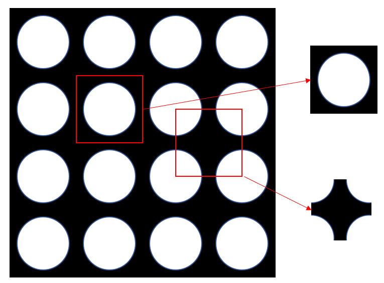
Figure 1: Locally periodic microstructures and unit cells.

Given a unit cell (microstructure) in 2D, a forward problem is to find its homogenized elasticity $3\times 3$ tensor $\bm{C}^{H}$. The theory of homogenization is well developed, for example, see Yang et al (2020); Hassani and Hinton (1998). A typical numerical strategy Andreassen and Andreasen (2014a) for computing $\bm{C}^{H}$ is to impose three independent periodic boundary conditions (in 2D), and solve the resulting finite element problems; see Figure 2. The stresses and strains from the three problems are then used to compute $\bm{C}^{H}$ as described in Andreassen and Andreasen (2014a).

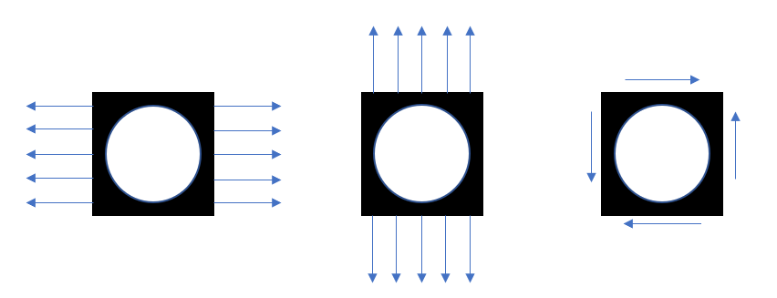
Figure 2: Extracting the elasticity tensor.

Next, various quantities of interest, namely, bulk modulus ($K$), shear modulus ($G$) and Poisson ratio ($\nu$) can be extracted from $\bm{C}^{H}$ as follows:

$$K=(C^{H}_{1,1}+C^{H}_{2,2}+C^{H}_{1,2}+C^{H}_{2,1})/4$$ (1a)

$$G=C^{H}_{3,3}$$ (1b)

$$\nu=(C^{H}_{2,1}+C^{H}_{1,2})/(C^{H}_{1,1}+C^{H}_{2,2})$$ (1c)

2.2 Microstructural Optimization Methods

The inverse problem is to arrive at an optimal topology that maximizes or minimizes one of these quantities of interest. There are several methods available today for optimizing microstructures; see, for example, Osanov and Guest (2016); Gao et al (2020); Vogiatzis et al (2017); Suresh (2014); Kollmann et al (2020); Guo and Buehler (2020).

In the popular density-based methods, one defines a pseudo-density $\rho_{e}\in(0,1]$ over the underlying finite element mesh. Then the microstructural optimization problem, of say, maximizing the bulk modulus, subject to a mass constraint (we prefer here a mass constraint over a volume constraint since this generalizes more easily to multiple materials), may be posed as follows:

$$\underset{\bm{\rho}}{\text{minimize}} -K(\bm{\rho})$$ (2a)

subject to $$\mathbf{K}(\bm{\rho})\bm{u}^{i}=\bm{f}^{i},i=1,2,3$$ (2b)

$$\sum_{e}\rho_{e}v_{e}\lambda_{e}=\hat{m}$$ (2c)

$$0<\rho_{e}\leq 1$$ (2d)

where $\mathbf{K}$ is the stiffness matrix, $\bm{u}^{i}$ and $\bm{f}^{i}$ are the displacement vector and the external force vector for the three problems in Figure  2, $v_{e}$ is the volume of the finite element, $\lambda_{e}$ is the physical density of the base material, and $\hat{m}$ is the mass constraint. In addition, the solid isotropic material with penalization (SIMP) penalization model is employed to link the density variables to the base material

$$E(\rho_{e})=E_{min}+E\rho_{e}^{p}$$ (3)

The field can now be optimized using, for example, optimality criteria Bendsoe and Sigmund (2003) or MMA Svanberg (1987), resulting in the desired microstructural topology; see Xia and Breitkopf (2015), for example. Similar problems can be posed, for example, to minimize the Poisson ratio, subject to a mass constraint.

3 Proposed Framework

3.1 Generalized Microstructural Problems

As stated earlier, in many applications, the mass constraint $\hat{m}$ (see Equation 2c) is not known a priori. Instead, it may be more advantageous to impose constraints on physical quantities. In this paper, we consider such generalized microstructural optimization problems of the form:

$$\underset{\bm{\rho}}{\text{minimize}} \phi(\bm{C}^{H}(\bm{\rho}))$$ (4a)

subject to $$\bm{K}(\bm{\rho})\bm{u}^{i}=\bm{f}^{i},i=1,2,3$$ (4b)

$$h_{j}(\bm{\rho})=0,j=1,2,...$$ (4c)

$$0<\bm{\rho}\leq 1$$ (4d)

where the objective $\phi(\bm{C}^{H})$ represents one of the following: the bulk modulus ($K$), shear modulus ($G$), Poisson ratio ($\nu$), or mass ($m$), and $h_{j}$ are equality constraints involving these quantities.

For example, the problem of maximizing the bulk modulus subject to a Poisson ratio constraint may be posed as:

$$\underset{\bm{\rho}}{\text{minimize}} -K(\bm{\rho})$$ (5a)

subject to $$\bm{K}(\bm{\rho})\bm{u}^{i}=\bm{f}^{i},i=1,2,3$$ (5b)

$$\nu(\bm{\rho})/\hat{\nu}-1=0$$ (5c)

$$0<\bm{\rho}\leq 1$$ (5d)

where $\hat{\nu}$ is the desired Poisson ratio. Similarly, the problem of minimizing the mass subject to constraints on the bulk modulus and Poisson ratio may be posed as:

$$\underset{\bm{\rho}}{\text{minimize}} m(\bm{\rho})$$ (6a)

subject to $$\bm{K}(\bm{\rho})\bm{u}^{i}=\bm{f}^{i},i=1,2,3$$ (6b)

$$K(\bm{\rho})/\hat{K}-1=0$$ (6c)

$$\nu(\bm{\rho})/\hat{\nu}-1=0$$ (6d)

$$0<\bm{\rho}\leq 1$$ (6e)

where $\hat{K}$ is the desired bulk modulus, and $\hat{\nu}$ is the desired Poisson ratio. In the remainder of this paper, we will consider solving such problems.

3.2 Representing Density using Neural Networks

One of the challenges in solving such generalized problems is computing the sensitivities of the objective and constraints. Manual derivation can be cumbersome and error-prone, especially when the problem is recast within the context of augmented Lagrangian formulation (see Section 3.3). We, therefore, propose here a neural-network (NN) framework that supports automatic sensitivity computation for gradient-based optimization Chandrasekhar et al (2021). The framework not only eliminates the burden of manual sensitivity calculations, it offers other computational advantages as discussed in the remainder of the paper.

In particular, we employ a simple fully-connected feed-forward neural network Bishop (2006). The input to the network are points ($x$, $y$) within the domain; the NN has a series of hidden layers associated with activation functions Goodfellow et al (2016), Lu et al (2019). The output is the density $\rho$ at that point; see Figure 3. Observe that the final layer is a SoftMax activation function Bishop (2006) that ensures that the density lies between 0 and 1. The density will depend on the weights and bias, i.e., they serve as the design variables $\bm{w}$.

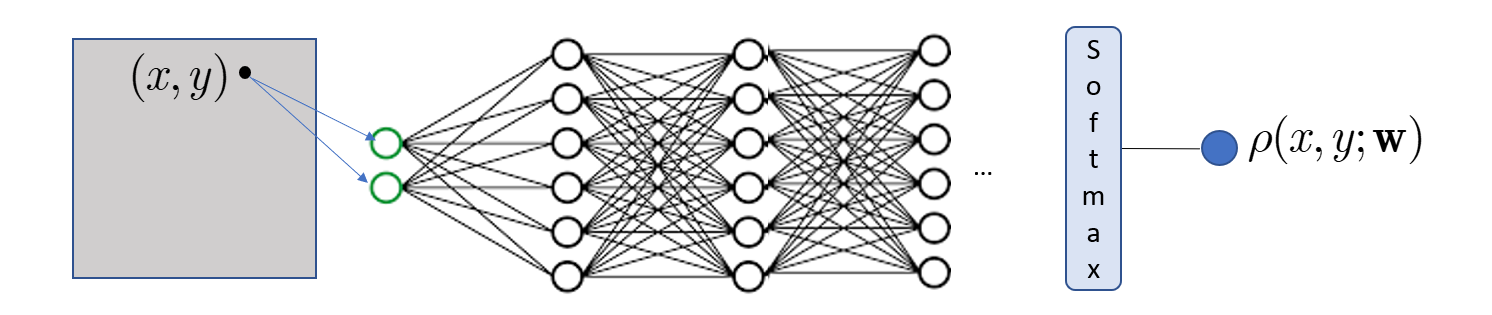
Figure 3: Neural network architecture for representing the density field.

Thus, we can now repose the generalized problem as:

$$\underset{\bm{w}}{\text{minimize}} \phi(\bm{C}^{H}(\bm{w}))$$ (7a)

subject to $$\bm{K}(\bm{w})\bm{u}^{i}=\bm{f}^{i},i=1,2,3$$ (7b)

$$h_{j}(\bm{w})=0,j=1,2,...n$$ (7c)

Observe that an explicit (bound) constraint on the density field is not needed since it is automatically satisfied by the Softmax function.

To generalize the above framework to multiple materials, the output of the NN is increased to $(M+1)$ variables, where $M$ is the number of non-void materials; see Figure 4. No other change is needed in the framework, i.e., one can use exactly the same number of design variables $\bm{w}$. Further, due to the nature of Softmax function, the partition of unity condition:

$$\sum\limits_{m=0}^{M}\rho_{m}=1$$ (8)

is automatically satisfied, i.e., the sum of all densities is guaranteed to be unity. Finally, the SIMP material model in Equation 3 is generalized to multiple materials as follows:

$$E(\rho)=E_{min}+\sum\limits_{m=0}^{M}E_{m}\rho_{m}^{p}$$ (9)

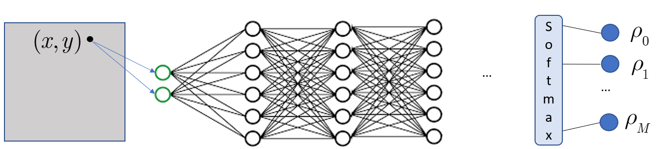
Figure 4: Neural network architecture for representing multiple materials.

3.3 Augmented Lagrangian

To solve both the single and multi-material problems, we will use the augmented Lagrangian method Nocedal and Wright (2006), i.e., let

$$L(\bm{w})=\phi+\sum\limits_{j=1,2...}^{n}{\alpha_{j}}h_{j}^{2}+\sum\limits_{j=1,2...}^{n}{\mu_{j}}h_{j}$$ (10)

where the penalty parameters $\alpha_{j}$ and Lagrange multipliers $\mu_{j}$ are updated through iterations. First, starting with a small value for $\alpha_{j}$ and a zero value for $\mu_{j}$ the augmented Lagrangian is minimized using the popular L-BFGS method Nocedal and Wright (2006). Then, the coefficients $\alpha$ and $\mu$ are updated as follows (see Section 4):

$${\alpha_{j}}^{(k+1)}={\alpha_{j}}^{(k)}+\Delta\alpha$$ (11a)

$${\mu_{j}}^{(k+1)}={\mu_{j}}^{(k)}+2{\alpha_{j}}^{(k+1)}h_{j}^{(k)}$$ (11b)

The optimization is repeated until convergence. For termination, we consider two quantities

$$\epsilon_{\phi}=\mid(\phi^{(k+1)}-\phi^{(k)})/\phi^{(k+1)}\mid$$ (12)

and

$$\epsilon_{h}=\sum\limits_{j=1,2...}^{n}\mid h_{j}\mid$$ (13)

The algorithm terminates when both quantities are less than a prescribed value (see Section 4 for details). The overall framework is illustrated in Figure 5.

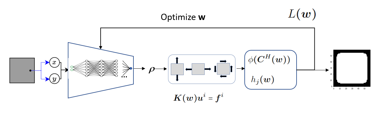
Figure 5: The optimization framework.

3.4 Algorithm

The algorithm for the proposed framework is described in algorithm 1. First, the target design objective $\phi$ and the set of equality constraints $h_{j}$ are specified along with an initial topology. Note that defining an initial topology is equivalent to initializing the neural network. Next, the domain is discretized into finite elements and the element centers serve as input to the neural network, which returns the elemental densities $\bm{\rho}$ as discussed in section 3.2. Homogenization is performed which predicts the homogenized structural response from the elemental densities as per section 2.1. Based on the results from homogenization, the objective $\phi$ eq. 7a and the constraints $h_{j}$ eq. 7c are evaluated. Next, the loss function $L$ is computed using eq. 10, and the gradient of the loss function with respect to the neural network weights ($\nabla L$) is computed through automatic differentiation. The NN is then trained using PyTorch’s L-BFGS optimizer as described in section 3.3, which requires the update of Lagrangian parameters $\alpha,\mu$. The training procedure continues until the convergence criteria are met.

Algorithm 1 Microstructural TO

1:procedure MicroTOuNN($\Omega_{0}$, $\phi$, …) $\ignorespaces\triangleright$ Inputs

2:     $\Omega^{0}\rightarrow\Omega^{0}_{h}$ $\ignorespaces\triangleright$ Domain discretization

3:     $\bm{x}=\{x_{e},y_{e}\}_{e\in\Omega^{0}_{h}}$ $\ignorespaces\triangleright$ elem centers; NN input

4:     k = 0; $\alpha_{i}=\alpha_{0}$; $\mu_{i}=0\;\forall i$ $\ignorespaces\triangleright$ Initialization (section 3.3)

5:     repeat $\ignorespaces\triangleright$ Optimization (Training)

6:         $NN(\bm{x}\mathchar 24635\relax\;\bm{w})\rightarrow\bm{\rho}$ $\ignorespaces\triangleright$ Fwd prop NN

7:         $\bm{\rho}\rightarrow\bm{C}^{H}$ $\ignorespaces\triangleright$ Homogenization (section 2.1)

8:         $\bm{C}^{H}\rightarrow\phi$ $\ignorespaces\triangleright$ Compute design objective eq. 7a

9:         $\{\bm{C}^{H},\bm{\rho}\}\rightarrow h_{j}$ $\ignorespaces\triangleright$ Compute constraints eq. 7c

10:         $\{\phi,h,\alpha_{i},\mu_{i}\}\rightarrow L$ $\ignorespaces\triangleright$ Loss from Equation 10

11:         $AD(L\leftarrow\bm{w})\rightarrow\nabla L$ $\ignorespaces\triangleright$ Auto diff for sensitivity

12:         $\bm{w}+\Delta\bm{w}(\nabla L)\rightarrow\bm{w}$ $\ignorespaces\triangleright$ L-BFGS step

13:         $\text{k}++$

14:         Update $\alpha_{i},\mu_{i}$ $\ignorespaces\triangleright$ Aug-Lag terms eq. 11a, eq. 11b

15:     until  $\Delta\phi<\hat{\epsilon}_{\phi}$ and $\Delta h<\hat{\epsilon}_{h}$ and $k<k_{max}$ $\ignorespaces\triangleright$ convg. criteria

16:     return $\bm{w}$

17:end procedure

4 Numerical examples

In this section, we conduct several numerical experiments to illustrate the proposed algorithm. The implementation is in Python, within the PyTorch environment. All experiments were conducted on an Intel i9-11900K @ 3.50GHz GHz, equipped with 32 GB of RAM. The default parameters are listed in Table 1. We use the popular SIMP continuation scheme Rojas2015Continuation for the material model. For the default NN configuration of 5 layers and 30 neurons per layer, the number of design variables $\bm{w}$ (weight and bias) is 3872.

Parameter	Description and default value
$E$, $\nu$	For base material: $E=1$, $\nu=0.3$; for void: $E=0.001$, $\nu=0.3$
$\lambda$(mass density)	For base material: $\lambda=1$; for void: $\lambda=0.001$
NN	Neural network: 5 layers and 30 neurons per layer, with Swish functions
$\alpha$, $\mu$	Lagrangian parameters: $\alpha_{0}=1,\Delta\alpha=5$ and $\mu_{0}=0$
$p$	SIMP continuation parameters: $p_{0}=2$, $\Delta p=0.5$, $p_{max}=10$
$n_{x}$,$n_{y}$	Mesh elements: $n_{x}=60$, $n_{y}=60$
$\hat{\epsilon}_{\phi}$, $\hat{\epsilon}_{h}$	Convergence criteria for objective and constraints: $\hat{\epsilon}_{\phi}$ = $\hat{\epsilon}_{h}$ = 0.025

Table 1: Default simulation parameters.

The default initial topology is a square block as illustrated in Figure 6.

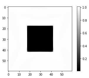
Figure 6: Default initial topology.

Through the experiments, we investigate the following:

1. Validation: First, we consider classic mass constrained optimization of bulk modulus, shear modulus, and Poisson ratio, and compare some of the computed values against well-established theoretical results.

2. Convergence: The typical convergence of the algorithm is then illustrated.

3. Initial Topology: Next, we consider initial topologies different from the one in Figure 6 and optimize for maximum bulk modulus.

4. Impact of NN Configuration: We then vary the NN size and consider its impact on Poisson ratio minimization.

5. Impact of Mesh Size: We repeat the above experiment but vary the mesh size instead of the NN size.

6. Generalized Problems: We then consider several generalized microstructural problems.

7. Multi-material design: Finally, we present results for multiple materials.

4.1 Validation

First, we consider the classic problem of bulk modulus maximization subject to a mass-fraction constraint of 0.3. The resulting topology, computed in 47 seconds, is illustrated in Figure 7(a). Similarly, Figure 7(b) illustrates a microstructure with maximal shear modulus for the same mass constraint, computed in 53 seconds. Finally, Figure 7(c) illustrates the microstructure when the Poisson ratio is minimized for the same mass constraint, computed in 55 seconds,

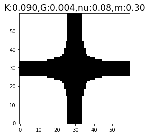
(a) Bulk modulus.

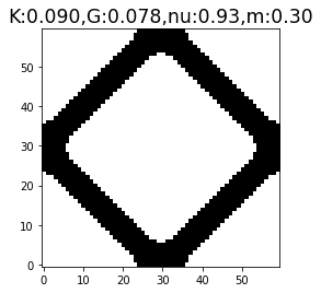
(b) Shear modulus.

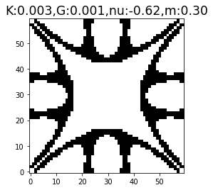
(c) Poisson ratio.

Figure 7: Classic microstructural optimization problems.

Table 2 compares the computed bulk modulus for various mass fractions, against the Hashin-Shtrikman upper bound.

$\hat{m}$	$K^{*}$	$K_{HS}$
0.1	0.020	0.0282
0.3	0.092	0.099
0.5	0.18	0.20
0.7	0.34	0.35

Table 2: Computed bulk modulus vs. HS upper bound.

4.2 Convergence

Recall that the error in the objective $\epsilon_{\phi}$ and error in the constraints $\epsilon_{g}$, defined in Equation 12 and Equation13 respectively, are computed at the end of every L-BFGS iteration. The algorithm terminates when $\epsilon_{\phi}<\hat{\epsilon}_{\phi}$ and $\epsilon_{g}<\hat{\epsilon}_{g}$ specified in Table 1. Figure 8(a) illustrates the objective error $\epsilon_{\phi}$ and the constraint error $\epsilon_{g}$ for bulk modulus maximization, while Figure 8(b) illustrates the two errors for Poisson ratio minimization.

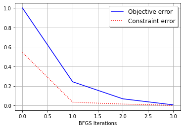
(a) Bulk modulus.

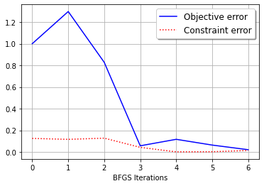
(b) Poisson ratio.

Figure 8: Objective and constraint errors after every L-BFGS iteration.

In the experiments, we observed that 3 to 20 L-BFGS iterations are sufficient. Further, each L-BFGS iteration typically involves 2 to 10 inner iterations. The homogenized properties are recorded at the end of every inner iteration. Figure 9(a) illustrates these quantities for bulk modulus maximization, and Figure 9(b) illustrates these for Poisson ratio minimization. The spikes observed in the two figures correspond to the start of a new L-BFGS iteration when the penalty parameters are updated.

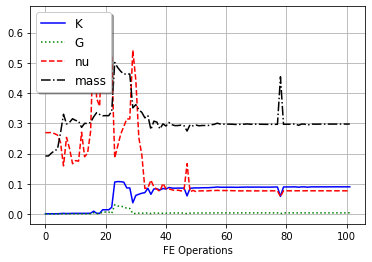
(a) Bulk modulus.

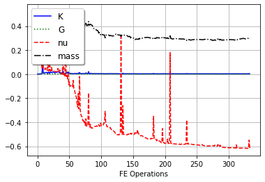
(b) Poisson ratio.

Figure 9: Various homogenized quantities after every FE operation.

4.3 Impact of Initial Topology

Next, we consider initial designs different from Figure 6 and study their impact on the optimal topology, with all other parameters are kept constant at default values. Specifically, we revisit the problem of maximizing the bulk modulus, subject to a mass-fraction constraint of 0.3.

For the initial topology of a circular hole in Figure 10(a), the final topology is illustrated in Figure 10(b).

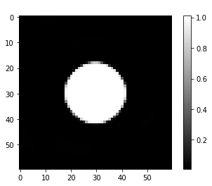
(a) Initial topology.

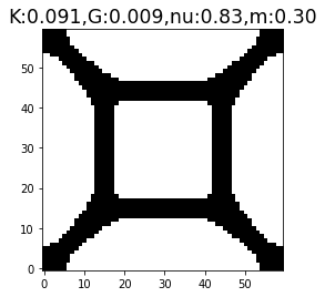
(b) Final topology.

Figure 10: Maximizing bulk modulus with mass constraint.

Similarly, with the initial topology of four circular holes in Figure 15(a), the final topology, for the same problem is illustrated in Figure 15(c), with $K^{*}=0.090$.

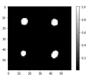
(a) Initial topology.

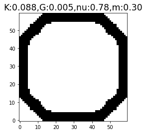
(b) Final topology.

Figure 11: Maximizing bulk modulus with mass constraint.

Although the designs are different, the final bulk moduli are comparable. Thus, one can potentially discover different designs by changing the initial design.

4.4 Impact of NN Size

We now vary the neural-network size and minimize the Poisson ratio, subject to a mass-fraction constraint of 0.3 (with default parameters). Figure 12 illustrates various designs obtained for different NN configurations. The final Poisson ratio $\nu^{*}$ for the three cases are -0.68, -0.62 and -0.84 respectively. The number of design variables are 492, 1782 and 11,682 respectively. We observe that as the number of design variables is increased, the algorithm tends to generate more complex designs. However, we did not observe any pattern between the NN size and the final objective achieved.

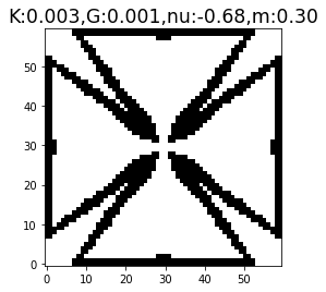
(a) NN: $5\times 10$.

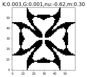
(b) NN: $5\times 20$.

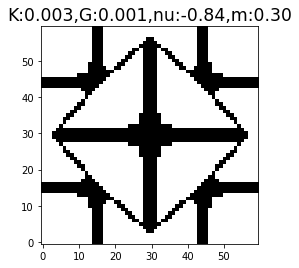
(c) NN: $8\times 40$.

Figure 12: Minimizing Poisson ratio with mass constraint using different NNs.

4.5 Impact of Mesh Size

Next, we vary the mesh size and minimize the Poisson ratio, subject to a mass constraint of 0.3 (with all other parameters at default). Figure 13 illustrates the designs obtained for different mesh sizes. The final Poisson ratio $\nu^{*}$ for the three cases are -0.56, -0.80 and -0.65 respectively. Once again, we did not observe any pattern between the mesh size and the final objective achieved.

(a) Mesh: $40\times 40$.

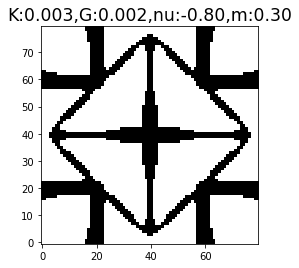
(b) Mesh: $80\times 80$.

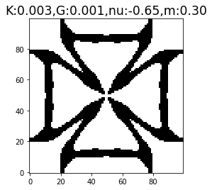
(c) Mesh: $100\times 100$.

Figure 13: Minimizing Poisson ratio for different mesh sizes.

4.6 Generalized Problems

To illustrate the benefits of the proposed framework, we first used the MATLAB code published in Xia and Breitkopf (2015) to minimize the Poisson ratio to a mass constraint of $\hat{m}=0.5$. The algorithm did not terminate; the final topology, after a maximum allowable 450 FE operations (15 seconds), is illustrated in Figure 14(a); it exhibits the following characteristics $\nu=-0.23$, $K=0.015$ and $G=0.002$. Observe that the microstructure is weak in bulk and shear.

In the proposed framework, the bulk modulus was maximized subject to $\nu=-0.23$ and $\hat{m}=0.5$, i.e., the constraints are consistent with the results obtained above. The resulting topology, after 420 FE operations (52 seconds), illustrated in Figure 14(b) exhibits the following characteristics $m=0.5$, $\nu=-0.23$, $K=0.043$ and $G=0.006$. Thus the proposed framework increases the bulk and shear moduli by a factor of $3X$. For approximately the same number of finite element operations, the proposed framework is slower due to the overhead of automatic differentiation.

Next, the shear modulus was maximized subject to $\nu=-0.23$ and $\hat{m}=0.5$. The resulting topology after 560 FE operations (91 seconds), illustrated in Figure 14(c) exhibits the following characteristics $m=0.5$, $\nu=-0.23$, $K=0.023$ and $G=0.029$, i.e., the bulk and shear moduli increased by a factor of $10X$.

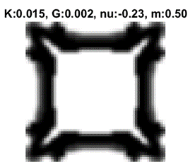
(a) Mass constrained.

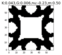
(b) Maximizing $K$.

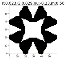
(c) Maximizing $G$.

Figure 14: Classic versus proposed framework.

One can also impose multiple physical constraints within the proposed framework. Consider the minimization of the mass, subject to bulk modulus and Poisson ratio constraints. Figure 15 illustrates three designs obtained for three different scenarios. The corresponding mass fractions are 0.33, 0.69, and 0.79.

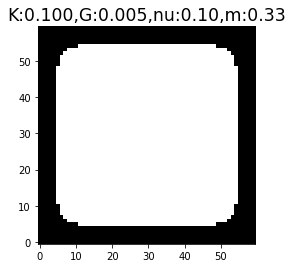
(a) $\hat{K}=0.1$, $\hat{\nu}=0.1$.

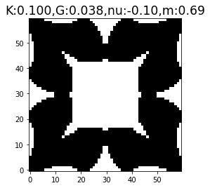
(b) $\hat{K}=0.1$, $\hat{\nu}=-0.1$.

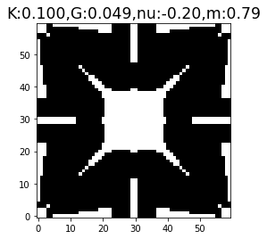
(c) $\hat{K}=0.1$, $\hat{\nu}=-0.2$.

Figure 15: Minimizing mass with bulk modulus and Poisson ratio constraints.

One can also target a specific elasticity matrix $\bm{\hat{C}}^{H}$. We consider a specific example from Yin and Yang (2001):

$$\bm{\hat{C}}^{H}=\begin{bmatrix}0.13&-0.03&0\\ -0.03&0.13&0\\ 0&0&0.015\end{bmatrix}$$ (14)

Note that there may exist multiple solutions (with significantly different masses) with the same $\bm{C}^{H}$ Vogiatzis et al (2017). Using our framework by imposing the target $\bm{C}^{H}$ and a target mass as constraints, one can obtain different designs; these are illustrated in Figure 16a and 16b, with mass target of 0.37 and 0.51, respectively. A solution, with a mass of 0.37 was reported in Yin and Yang (2001); see Figure 16c.

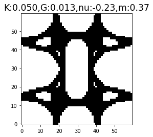
(a) m = 0.37

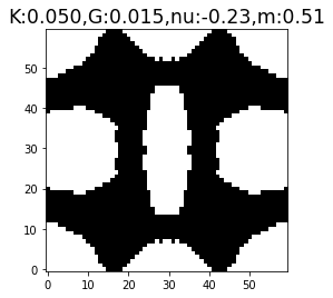
(b) m = 0.51

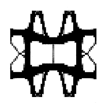
(c) m = 0.37 Yin and Yang (2001)

Figure 16: Designs obtained for a targeted $\bm{\hat{C}}^{H}$.

4.7 Sampling at Higher Resolution

Once the optimization is completed, the global representation of the density field via the NN allows us to sample the field at a finer resolution and extract a high-resolution topology at no additional cost. This is illustrated in Figure 17. Observe that directly smoothing the coarse topology will retain the original topological features. However, sampling at a high resolution can recover topological features captured by the NN, as can be observed in Figure 17.

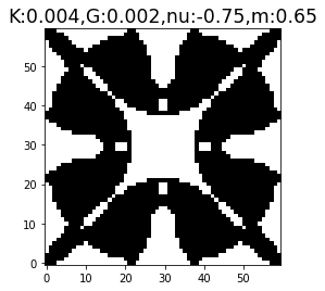
(a) Raw output.

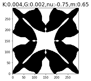
(b) Sampling at higher resolution.

Figure 17: Sampling the neural network at a higher resolution.

4.8 Multiple Materials

Next consider maximization of $K$, subject to a mass constraint ($\hat{m}=0.3$), with two, three and four materials. The material properties are summarized in Table 3.

Material	Color code	$E$	$\nu$	$\lambda$
0	White	0.001	0.3	0
1	Black	1	0.3	1
2	Red	0.2	0.3	0.2
3	Green	0.3	0.3	0.25
3	Blue	0.4	0.3	0.3

Table 3: Material properties.

The results are illustrated in Figure 18 (compare against Figure 7(a) for single material). The final bulk modulus $K^{*}$ for the three cases are 0.172, 0.225 and 0.240, respectively (compared to 0.091 for single material). Observe that the bulk modulus increases as additional materials are introduced.

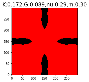
(a) Two materials.

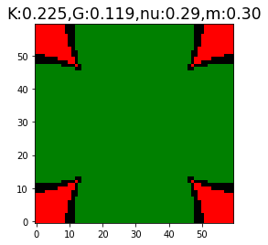
(b) Three materials.

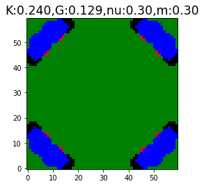
(c) Four materials.

Figure 18: Maximizing $K$ with mass constraint using multiple materials.

5 Conclusions

This paper presents a generalized neural-network-based framework for microstructural optimization where any of the microstructural quantities, namely, bulk, shear, Poisson ratio, volume or mass, can serve as the objective, while the remaining can be subject to constraints. The error-prone task of sensitivity computation was avoided by exploiting NN’s backward propagation. Further, for designing NPR materials, we avoided the use of specialized optimization techniques and heuristics; instead, standard L-BFGS optimization was used. The framework was demonstrated using several numerical experiments. Due to the overhead cost of automatic differentiation (AD), the framework was found to be slower than, say, the MATLAB implementation presented in Xia and Breitkopf (2015). However, we believe the benefits of AD outweigh the computational costs.

There are several directions for future research: extension to multi-physics Das and Sutradhar (2020), 3D Andreassen and Andreasen (2014b), geometric and material non-linearity Wallin and Tortorelli (2020), inclusion of stress constraints Collet et al (2018), multi-stable materials Yang and Ma (2020), and inclusion of manufacturing constraints Du et al (2018).

Compliance with ethical standards

The authors declare that they have no conflict of interest.

Replication of Results

The Python code pertinent to this paper is available at https://github.com/UW-ERSL/MicroTOuNN.

References

- \bibcommenthead
- Andreassen and Andreasen (2014a) Andreassen E, Andreasen CS (2014a) How to determine composite material properties using numerical homogenization. Computational Materials Science 83:488–495
- Andreassen and Andreasen (2014b) Andreassen E, Andreasen CS (2014b) How to determine composite material properties using numerical homogenization. Computational Materials Science 83:488–495. 10.1016/j.commatsci.2013.09.006
- Asadpoure et al (2017) Asadpoure A, Tootkaboni M, Valdevit L (2017) Topology optimization of multiphase architected materials for energy dissipation. Computer Methods in Applied Mechanics and Engineering 325:314–329
- Bendsoe and Sigmund (2003) Bendsoe MP, Sigmund O (2003) Topology optimization: theory, methods, and applications, 2nd edn. Springer Berlin Heidelberg, 10.1063/1.3278595
- Bishop (2006) Bishop CM (2006) Pattern recognition and machine learning. springer
- Chandrasekhar et al (2021) Chandrasekhar A, Sridhara S, Suresh K (2021) Auto: a framework for automatic differentiation in topology optimization. Structural and Multidisciplinary Optimization 64(6):4355–4365. 10.1007/s00158-021-03025-8, URL https://doi.org/10.1007/s00158-021-03025-8
- Collet et al (2018) Collet M, Noël L, Bruggi M, et al (2018) Topology optimization for microstructural design under stress constraints. Structural and Multidisciplinary Optimization 58(6):2677–2695
- Das and Sutradhar (2020) Das S, Sutradhar A (2020) Multi-physics topology optimization of functionally graded controllable porous structures: Application to heat dissipating problems. Materials & Design 193:108,775
- Du et al (2018) Du Z, Zhou XY, Picelli R, et al (2018) Connecting microstructures for multiscale topology optimization with connectivity index constraints. Journal of Mechanical Design 140(11):111,417
- Gao et al (2020) Gao J, Li H, Luo Z, et al (2020) Topology optimization of micro-structured materials featured with the specific mechanical properties. International Journal of Computational Methods 17(03):1850,144
- Goodfellow et al (2016) Goodfellow I, Bengio Y, Courville A (2016) Deep Learning. MIT Press
- Guest and Prévost (2006) Guest JK, Prévost JH (2006) Optimizing multifunctional materials: design of microstructures for maximized stiffness and fluid permeability. International Journal of Solids and Structures 43(22-23):7028–7047
- Guo and Buehler (2020) Guo K, Buehler MJ (2020) A semi-supervised approach to architected materials design using graph neural networks. Extreme Mechanics Letters 41:101,029
- Hassani and Hinton (1998) Hassani B, Hinton E (1998) A review of homogenization and topology optimization i—homogenization theory for media with periodic structure. Computers & Structures 69(6):707–717
- Hsieh et al (2021) Hsieh MT, Begley MR, Valdevit L (2021) Architected implant designs for long bones: Advantages of minimal surface-based topologies. Materials & Design 207:109,838
- Kollmann et al (2020) Kollmann HT, Abueidda DW, Koric S, et al (2020) Deep learning for topology optimization of 2d metamaterials. Materials & Design 196:109,098
- Lu et al (2019) Lu L, Shin Y, Su Y, et al (2019) Dying relu and initialization: Theory and numerical examples. arXiv preprint arXiv:190306733
- Nocedal and Wright (2006) Nocedal J, Wright S (2006) Numerical optimization. Springer Science & Business Media
- Osanov and Guest (2016) Osanov M, Guest JK (2016) Topology optimization for architected materials design. Annual Review of Materials Research 46:211–233
- Sigmund (1994) Sigmund O (1994) Materials with prescribed constitutive parameters: an inverse homogenization problem. International Journal of Solids and Structures 31(17):2313–2329
- Sigmund and Søndergaard Jensen (2003) Sigmund O, Søndergaard Jensen J (2003) Systematic design of phononic band–gap materials and structures by topology optimization. Philosophical Transactions of the Royal Society of London Series A: Mathematical, Physical and Engineering Sciences 361(1806):1001–1019
- Suresh (2014) Suresh K (2014) Efficient microstructural design for additive manufacturing. In: ASME 2014 International Design Engineering Technical Conferences and Computers and Information in Engineering Conference, 10.1115/DETC201434383
- Svanberg (1987) Svanberg K (1987) The method of moving asymptotes—a new method for structural optimization. International journal for numerical methods in engineering 24(2):359–373
- Vogiatzis et al (2017) Vogiatzis P, Chen S, Wang X, et al (2017) Topology optimization of multi-material negative poisson’s ratio metamaterials using a reconciled level set method. Computer-Aided Design 83:15–32
- Wallin and Tortorelli (2020) Wallin M, Tortorelli DA (2020) Nonlinear homogenization for topology optimization. Mechanics of Materials 145:103,324
- Xia and Breitkopf (2015) Xia L, Breitkopf P (2015) Design of materials using topology optimization and energy-based homogenization approach in matlab. Structural and multidisciplinary optimization 52(6):1229–1241
- Yang and Ma (2020) Yang H, Ma L (2020) 1d to 3d multi-stable architected materials with zero poisson’s ratio and controllable thermal expansion. Materials & Design 188:108,430
- Yang et al (2020) Yang H, Abali BE, Timofeev D, et al (2020) Determination of metamaterial parameters by means of a homogenization approach based on asymptotic analysis. Continuum mechanics and thermodynamics 32(5):1251–1270
- Yin and Yang (2001) Yin L, Yang W (2001) Optimality criteria method for topology optimization under multiple constraints. Computers & Structures 79(20-21):1839–1850
- Zhou and Li (2008) Zhou S, Li Q (2008) Computational design of multi-phase microstructural materials for extremal conductivity. Computational Materials Science 43(3):549–564