Kinematics and Mass Distributions for
Non-Spherical Deprojected Sérsic Density Profiles
and Applications to Multi-Component Galactic Systems

Using kinematics to decompose galaxies’ mass profiles, including the dark matter contribution, often requires parameterization of the baryonic mass distribution based on ancillary information. One such model choice is a deprojected Sérsic profile with an assumed intrinsic geometry. The case of flattened, deprojected Sérsic models has previously been applied to flattened bulges in local star-forming galaxies (SFGs), but can also be used to describe the thick, turbulent disks in distant SFGs. Here we extend this previous work that derived density ($\rho$) and circular velocity ($v_{\mathrm{circ}}$) curves by additionally calculating the spherically-enclosed 3D mass profiles ($M_{\mathrm{sph}}$). Using these profiles, we compare the projected and 3D mass distributions, quantify the differences between the projected and 3D half-mass radii ($R_{\mathrm{e}}$; $r_{1/2,\mathrm{mass,3D}}$), and present virial coefficients relating $v_{\mathrm{circ}}(R)$ and $M_{\mathrm{sph}}(<r=R)$ or $M_{\mathrm{tot}}$. We then quantify differences between mass fraction estimators for multi-component systems, particularly for dark matter fractions (ratio of squared circular velocities versus ratio of spherically enclosed masses), and consider the compound effects of measuring dark matter fractions at the projected versus 3D half-mass radii. While the fraction estimators produce only minor differences, using different aperture radius definitions can strongly impact the inferred dark matter fraction. As pressure support is important in analysis of gas kinematics (particularly at high redshifts), we also calculate the self-consistent pressure support correction profiles, which generally predict less pressure support than for the self-gravitating disk case. These results have implications for comparisons between simulation and observational measurements, and for the interpretation of SFG kinematics at high redshifts. A set of precomputed tables and the code to calculate the profiles are made publicly available.

Table 1: Definitions of key variables

Variable	Definition	Reference
	— Model —
$n$	Sérsic index	Sec. 2.1
$R_{\mathrm{e}}$	Projected 2D Sérsic effective radius	Sec. 2.1
$q_{0}$	Intrinsic axis ratio $c/a$	Sec. 2.1
gray	— Geometry —
$R$	Radius in the midplane	Sec. 2.1
$z$	Height above the midplane	Sec. 2.1
$m=\sqrt{R^{2}+(z/q_{0})^{2}}$	Spheroid isodensity surface distance	Sec. 2.1
	— Derived —
$\rho(m)$	3D deprojected density	Sec. 2.1
$v_{\mathrm{circ}}(R)$	Circular velocity in the midplane, accounting for non-spherical potentials	Sec. 2.2
$M_{\mathrm{sph}}(<r=R)$	Mass enclosed within a sphere of radius $r=R$	Sec. 2.3
$M_{\mathrm{spheroid}}(<m=R)$	Mass enclosed within spheroid with isodensity surface distance $m=R$ and intrinsic axis ratio $q_{0}$	Sec. 2.3
$r_{1/2,\mathrm{mass,3D}}$	3D spherical half-mass radius (assuming constant $M/L$)	Sec. 2.4
$k_{\mathrm{3D}}(R_{\mathrm{e}})$	3D enclosed mass virial coefficient relating $v_{\mathrm{circ}}(R)$ to $M_{\mathrm{sph}}(<r=R)$	Sec. 3
$k_{\mathrm{tot}}(R)$	Total virial coefficient relating $v_{\mathrm{circ}}(R)$ to $M_{\mathrm{tot}}$	Sec. 3
$f_{\mathrm{DM}}^{m}(R)$	Dark matter fraction defined as ratio of dark matter to total mass enclosed within a sphere of radius $r=R$	Sec. 4.2
$f_{\mathrm{DM}}^{v}(R)$	Dark matter fraction defined as ratio of dark matter to total circular velocities squared at radius $R$	Sec. 4.2
$\alpha(R)$	Pressure support correction ($=\mathrm{d}\ln\rho_{g}/\mathrm{d}\ln{}R$ for constant dispersion)	Sec. 5.1
black

1 Introduction

Galaxy kinematics, such as rotation curves, are a powerful tool to measure the mass of all components in a galaxy (e.g., van der Kruit & Allen 1978, Courteau et al. 2014). Notably, this technique has been used to study the dark matter content of galaxies at a wide range of epochs, including constraints on the halo profile shapes (e.g., Sofue & Rubin 2001, de Blok 2010, Genzel et al. 2020, among many others). Furthermore, by using kinematics to probe the mass and angular momentum distribution within galaxies, it is possible to constrain the processes regulating galaxy growth and evolution over time (van der Kruit & Freeman 2011, Förster Schreiber & Wuyts 2020; see also, e.g., Mo et al. 1998, Sofue & Rubin 2001, Romanowsky & Fall 2012). It is especially informative to study the kinematics of star-forming galaxies (SFGs), which tend to lie on a tight “star-forming main sequence” where much of cosmic star formation occurs (Speagle et al. 2014; Rodighiero et al. 2011, Whitaker et al. 2014, Tomczak et al. 2016). However, there are challenges to recovering the intrinsic mass properties of galaxies from their observed kinematics.

One such challenge is that in order to overcome degeneracies in kinematic mass decomposition (particularly when including an unseen dark component; e.g., van Albada et al. 1985), separate constraints on the baryonic (gas and stellar) component are needed, either through empirical measurements or with a choice of parameterization (e.g., Persic et al. 1996, de Blok & McGaugh 1997, Palunas & Williams 2000, Dutton et al. 2005, de Blok et al. 2008, Courteau et al. 2014). Multi-wavelength imaging and spectroscopy (in emission or absorption) can constrain the distribution of gas and stars in galaxies. Such observations of individual galaxies provide projected information and not the 3D quantities needed for kinematic modeling. Consequently, it is often necessary to first parameterize the projected distributions and then make reasonable assumptions about the galaxies’ intrinsic geometries in order to deproject the surface distributions into 3D mass profiles.

Observationally, the light distributions of galaxies are often described by Sérsic (1968) profiles (e.g., Peng et al. 2002, 2010, Simard et al. 2002, 2011, Blanton et al. 2003, Wuyts et al. 2011, van der Wel et al. 2012, Conselice 2014, and numerous others). In some cases, there are distinct components within galaxies, but these are also frequently described by Sérsic profiles with distinct indices $n$ and effective radii $R_{\mathrm{e}}$ (e.g., a disk and bulge for star-forming galaxies; Courteau et al. 1996, Bruce et al. 2012, Lang et al. 2014). Thus, Sérsic profiles are a natural choice for the projected parameterization.

Deprojections of Sérsic profiles have been studied in numerous previous works, for spherical (e.g., Ciotti 1991, Ciotti & Lanzoni 1997, Baes & Ciotti 2019a, b), triaxial (e.g., Stark 1977, Trujillo et al. 2002), and axisymmetric geometries (e.g., Noordermeer 2008). Additionally, the dynamics for exponential surface profiles have been derived for both razor-thin (Freeman 1970) and finitely thick (Casertano 1983) geometries (though these are generalizable to arbitrary Sérsic index; e.g., see Binney & Tremaine 2008). These intrinsic geometries have applications for various galaxies or galaxy components, depending on the galaxy properties and epoch.

In particular, the mass distribution geometry of SFGs changes over time. Nearby SFGs often have thin disks, particularly in the gas components (van der Kruit & Freeman 2011), while distant (massive) SFGs tend to have thick, turbulent disks (Glazebrook 2013, Förster Schreiber & Wuyts 2020, and references therein). While more observations are needed to better constrain the vertical disk structure of distant, massive SFGs, flattened (oblate) distributions are more appropriate models (as adopted by, e.g., Wuyts et al. 2016, Genzel et al. 2017, 2020), using the same geometric deprojection used by Noordermeer (2008) to describe the flattening of nearby bulges.

A second challenge is that the observed rotation must be corrected for pressure support. This correction is important for gas kinematic measurements, especially at high redshifts where disks have high gas turbulence. A number of works have considered different analytic prescriptions for correcting for the pressure support in gas kinematics (e.g., Weijmans et al. 2008, Burkert et al. 2010, Dalcanton & Stilp 2010, Kretschmer et al. 2021). In general, such corrections require measurements of the gas turbulence $\sigma$ from spatially-resolved spectroscopy (i.e., slit along the major axis or kinematic maps) as well as constraints or parameterizations of the gas density profile. If deprojected Sérsic distributions are used to model the mass and $v_{\mathrm{circ}}$ profiles for galaxies’ gas and stellar components, then a pressure support prescription derived using the density slope can be adopted for a self-consistent kinematic analysis (as in, e.g., Weijmans et al. 2008, Burkert et al. 2010, Dalcanton & Stilp 2010). If galaxies exhibit non-constant dispersion, support from dispersion gradients or anisotropy can also be included (e.g., Weijmans et al. 2008, Dalcanton & Stilp 2010).

In order to further consider implications for the interpretation of the kinematics of high-redshift SFGs modeled using deprojected, flattened Sérsic profiles, in this paper we revisit and extend the framework first presented by Noordermeer (2008, hereafter N08). We first present various profile derivations for deprojected, flattened Sérsic profiles, including the density and circular velocity profiles determined by N08 as well as the spherically-enclosed 3D mass profiles (Sec. 2). Using the calculated profiles, we examine the relationship between projected 2D and 3D mass distributions, including differences between the 2D $R_{\mathrm{e}}$ and 3D $r_{1/2,\mathrm{mass,3D}}$ (Sec. 2.4). The circular velocity and 3D mass distributions are also used to calculate virial coefficients (Sec. 3). Next, we examine the circular velocity and enclosed mass profiles for multi-component systems for a range of realistic $z\sim 2$ galaxy properties (Sec. 4). We find the composite baryonic 3D half-mass radius $r_{1/2,\mathrm{3D,baryons}}$ is often smaller than the projected disk effective radius $R_{\mathrm{e,disk}}$. While different dark matter fraction estimators $f_{\mathrm{DM}}^{v}$ (the ratio of the dark matter to total circular velocities squared) and $f_{\mathrm{DM}}^{m}$ (the ratio of the dark matter to total mass enclosed within a sphere) are similar when calculated at the same radius, large differences in $f_{\mathrm{DM}}$ can result from the use of different aperture radii ($r_{1/2,\mathrm{3D,baryons}}$ vs. $R_{\mathrm{e,disk}}$). We then determine the self-consistent turbulent pressure support correction, assuming a constant $\sigma_{0}$, which is typically only half the amount predicted for a self-gravitating disk, and demonstrate the correction for a range of realistic $z\sim 2$ galaxy properties (Sec. 5). Finally, we discuss these results and their implications, in particular for comparisons between simulations and observations and for studies of disk galaxy kinematics at $z\sim 1-3$ (Sec. 6). We highlight how typical observational and simulation “half-mass” radius estimates can lead to differences of up to $\sim 0.15$ in measured $f_{\mathrm{DM}}$, and how the lower pressure support correction derived for these mass distributions (compared to the self-gravitating disk prescription) would imply typically lower inferred $f_{\mathrm{DM}}$ from observations.

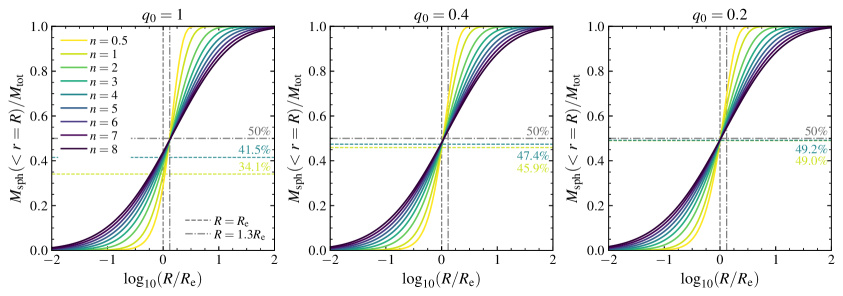
Figure 1: Fractional mass enclosed within a sphere of radius $r=R$ for deprojected Sérsic models of different intrinsic axis ratios. From left to right, the enclosed $M_{\mathrm{sph}}$ is plotted as a function of log radius (relative to the projected 2D effective radius, $R_{\mathrm{e}}$), assuming intrinsic axis ratios of $q_{0}=1,0.4,0.2$, respectively. The colored curves denote the enclosed mass profiles for Sérsic indices from $n=0.5$ to $n=8$ (yellow to purple). The vertical lines denote $R=R_{\mathrm{e}}$ (grey dashed) and $R=1.3R_{\mathrm{e}}$ ($\approx r_{1/2,\mathrm{mass,3D}}$ for $q_{0}=1$; grey dashed dotted), and the horizontal colored lines denote the fraction of the mass enclosed within $r=R_{\mathrm{e}}$ for $n=1,4$ (lime, teal dashed, respectively) and 50% of the total mass (grey dashed dotted). For $q_{0}=1$, the half-mass 3D spherical radius is indeed $r_{1/2,\mathrm{mass,3D}}\approx 1.3R_{\mathrm{e}}$ regardless of $n$, as in Ciotti (1991). For flattened (i.e., oblate) systems, the half-mass 3D spherical radius is smaller, and approaches $R_{\mathrm{e}}$ as $q_{0}$ decreases. See also Fig. 2.

A set of tables containing precomputed profiles and values — including $v_{\mathrm{circ}}(R)$ (Eq. 5), $M_{\mathrm{sph}}(\mbox{$<r=R$})$ (Eq. 8), $M_{\mathrm{spheroid}}(\mbox{$<m=R$})$ (Eq. 6), $\rho(r=R)$ (Eq. 2), $\mathrm{d}\ln\rho/\mathrm{d}\ln{}R$ (derived from Eq. 17), $r_{1/2,\mathrm{mass,3D}}$, $k_{\mathrm{tot}}(R_{\mathrm{e,disk}})$ (Eq. 10), and $k_{\mathrm{3D}}(R_{\mathrm{e,disk}})$ (Eq. 9) — for a range of intrinsic axis ratios $q_{0}$ and Sérsic indices, and the code used to compute the profiles, are made available. For reference, key variables and their definitions are listed in Table Kinematics and Mass Distributions for Non-Spherical Deprojected Sérsic Density Profiles and Applications to Multi-Component Galactic Systems.

We assume a flat $\Lambda$CDM cosmology with $\Omega_{m}=0.3$, $\Omega_{\Lambda}=0.7$, and $H_{0}=70\mathrm{\,km\ s^{-1}\ Mpc^{-1}}$.

2 Derivation of mass profiles and rotation curves

In this section, we present formulae for the mass profiles and rotation curves for models whose projected intensity distributions follow Sérsic profiles, but that have oblate (flattened) or prolate axisymmetric 3D density distributions (i.e., the isodensity contours follow oblate/prolate spheroids), following the deprojection derivation of N08.

2.1 Deprojected Sérsic density profile

We assume that the mass density of the 3D spheroid can be written as $\rho(x,y,z)=\rho(m)$, where $(m/a)^{2}=(x/b)^{2}+(y/a)^{2}+(z/c)^{2}$ specifies the isodensity surfaces for a given set of semi-axis lengths $a,b,c$. For an axisymmetric system this simplifies to $m=\sqrt{R^{2}+(z/q_{0})^{2}}$, where $R=\sqrt{x^{2}+y^{2}}$ is the distance in the plane of axisymmetry, $z$ is the distance from the midplane, the semi axes $a=b$, and $q_{0}=c/a$ is the intrinsic axis ratio of the spheroid. To project the intrinsic galaxy coordinates to the observer’s frame, we adopt the transformation from $(x,y,z)$ to $(\zeta,\kappa,\xi)$ from Eq. 1 of N08, where $\zeta$ lies along the line-of-sight, $\kappa$ and $\xi$ lie along the galaxy major and minor axes (as viewed in the sky plane, for oblate geometries; i.e., $\kappa=a$), respectively, and $i$ is the inclination of the system relative to the observer (see also Fig. 1 of N08). The observed axis ratio of the ellipsoid is then $q_{\mathrm{obs}}=\sqrt{q_{0}^{2}+(1-q_{0}^{2})\cos^{2}i}$.

Within the observer’s coordinate frame, the relationship between the 3D mass density profile and the projected light intensity along the major axis of the galaxy is ($\xi=0$; from Eq. 8 of N08):

$$I(\kappa)=2\frac{q_{0}}{q_{\mathrm{obs}}}\int_{\kappa}^{\infty}\frac{1}{\Upsilon(m)}\rho(m)\frac{m\,\mathrm{d}{}m}{\sqrt{m^{2}-\kappa^{2}}},$$ (1)

where $\Upsilon(m)$ is the mass-to-light ratio of the galaxy and $q_{\mathrm{obs}}/q_{0}=\sqrt{\sin^{2}i+(1/q_{0}^{2})\cos^{2}i}$. For simplicity, we assume a constant mass-to-light ratio, $\Upsilon(m)\equiv\Upsilon$.

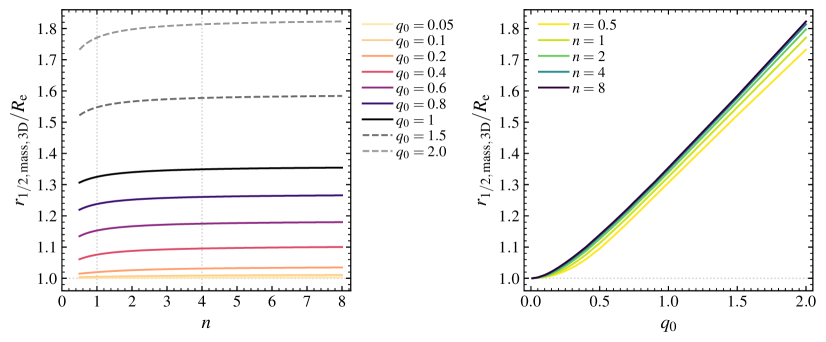
Figure 2: Comparison between the 3D spherical half-mass radius, $r_{1/2,\mathrm{mass,3D}}$ and the projected 2D effective radius, $R_{\mathrm{e}}$, for a range of Sérsic indices $n$ and intrinsic axis ratios $q_{0}$ (left, colored by $q_{0}$; right, colored by $n$). For oblate cases, $R_{\mathrm{e}}$ is the projected major axis, while for prolate cases $R_{\mathrm{e}}$ is the projected minor axis. For all cases, $r_{1/2,\mathrm{mass,3D}}>R_{\mathrm{e}}$. However, as $q_{0}$ decreases (i.e., flatter Sérsic distributions), the 3D half-mass radius approaches the value of $R_{\mathrm{e}}$. Overall, the systematic difference between $r_{1/2,\mathrm{mass,3D}}$ and $R_{\mathrm{e}}$ emphasizes that, while half of the model mass is enclosed within a projected 2D ellipse of major axis $R_{\mathrm{e}}$ (e.g., an infinite ellipsoidal cylinder), less than half the total mass is enclosed within a sphere of radius $R_{\mathrm{e}}$ (ignoring any $M/L$ gradients or optically thick regions, which would change $R_{e,\mathrm{light}}/R_{e,\mathrm{mass}}$).

The deprojected density profile is found by inverting this Abel integral, with (c.f. Eq. 9, N08)

$$\rho(m)=-\frac{\Upsilon}{\pi}\frac{q_{\mathrm{obs}}}{q_{0}}\int_{m}^{\infty}\frac{\mathrm{d}{}I}{\mathrm{d}{}\kappa}\frac{\mathrm{d}{}\kappa}{\sqrt{\kappa^{2}-m^{2}}}.$$ (2)

We write the Sérsic profile as (c.f. Eq. 11, N08)

$$I(\kappa)=I_{e}\exp\left\{-b_{\mathrm{n}}\left[\left(\frac{\kappa}{R_{\mathrm{e}}}\right)^{1/n}-1\right]\right\},$$ (3)

where $R_{\mathrm{e}}$ is the effective radius, $n$ is the Sérsic index, $I_{e}$ is the surface brightness at $R_{\mathrm{e}}$, and $b_{\mathrm{n}}$ satisfies $\gamma(2n,b_{\mathrm{n}})=\frac{1}{2}\,\Gamma(2n)$, where $\Gamma(a)$ and $\gamma(a,x)$ are the regular and lower incomplete gamma functions, respectively (e.g., Graham & Driver 2005).

The derivative is then

$$\frac{\mathrm{d}{}I}{\mathrm{d}{}\kappa}=-\frac{I_{e}b_{\mathrm{n}}}{nR_{\mathrm{e}}}\exp\left\{-b_{\mathrm{n}}\left[\left(\frac{\kappa}{R_{\mathrm{e}}}\right)^{1/n}-1\right]\right\}\left(\frac{\kappa}{R_{\mathrm{e}}}\right)^{(1/n)-1}.$$ (4)

By inserting Eq. 4 into Eq. 2, we can numerically integrate to obtain the deprojected density profile $\rho(m)$. For the adopted convention here, where the projected $\kappa$ lies along $a$ in the midplane (so this is the usual projected major axis for oblate cases but is the projected minor axis for prolate cases), we have $R_{\mathrm{e}}=a$ as the projected effective radius.

2.2 Rotation curves

Next we determine the circular rotation curve for this class of density profiles, following the derivation of Binney & Tremaine (2008, Eq. 2.132; also Eq. 10, N08). The circular rotation curve at the midplane of the galaxy is thus

$$\begin{split}v_{\mathrm{circ}}^{2}(R)=-&4Gq_{\mathrm{obs}}\Upsilon\\ \times\int_{m=0}^{R}&\left[\int_{\kappa=m}^{\infty}\frac{\mathrm{d}{}I}{\mathrm{d}{}\kappa}\frac{\mathrm{d}{}\kappa}{\sqrt{\kappa^{2}-m^{2}}}\right]\frac{m^{2}\,\mathrm{d}{}m}{\sqrt{R^{2}-(1-q_{0}^{2})m^{2}}}.\end{split}$$ (5)

As noted by N08, this equation is valid for any observed intensity profile $I(\kappa)$. Here we combine Eqs. 2 and 5, which can be numerically integrated to yield $v_{\mathrm{circ}}(R)$.

2.3 Enclosed 3D mass

We next derive the enclosed mass for models with the density profiles given above. Given the modified coordinate $m$, the mass enclosed within a spheroid with intrinsic axis ratio $q_{0}$ can be expressed as

$$\begin{split}M_{\mathrm{spheroid}}&(<m=R)\equiv M_{\mathrm{3D,spheroid}}(<m=R)\\ &=4\pi q_{0}\int_{0}^{R}m^{2}\,\mathrm{d}{}m\,\rho(m)\,\,.\end{split}$$ (6)

Integrated to infinity, this is equivalent to the total luminosity of the Sérsic profile times the constant assumed mass-to-light ratio, or $M_{\mathrm{tot}}=\Upsilon L_{\mathrm{tot}}$, so the intensity normalization for a flattened Sérsic profile with observed axis ratio $q_{\mathrm{obs}}$ is

$$I_{e}=\frac{M_{\mathrm{tot}}}{\Upsilon{}}\,\frac{1}{q_{\mathrm{obs}}}\,\frac{b_{\mathrm{n}}^{2n}}{2\pi{}R_{\mathrm{e}}^{2}n\,e^{b_{\mathrm{n}}}\,\Gamma(2n)}\,\,.$$ (7)

However, there may be situations where we wish to compute the mass enclosed within a sphere of radius $r=\sqrt{R^{2}+z^{2}}$ instead of within a flattened (or prolate) spheroid. We thus use a change of coordinates to calculate the spherical enclosed mass:

$$\begin{split}M_{\mathrm{sph}}&(<r=R)\equiv M_{\mathrm{3D,sphere}}(<r=R)\\ &=4\pi\int_{\tilde{R}\,=\,0}^{R}\tilde{R}\;\mathrm{d}{}\tilde{R}\int_{z\,=\,0}^{q_{0}\sqrt{R^{2}\,-\,\tilde{R}\,^{2}}}\rho\left(\!\!\sqrt{\tilde{R}\,^{2}+(z/q_{0})^{2}}\right)\mathrm{d}{}z,\end{split}$$ (8)

using $\rho(m)$ from Eq. 2, with $m=\sqrt{\tilde{R}\,^{2}+(z/q_{0})^{2}}$. This integral can be numerically evaluated to find the 3D spherical enclosed mass profile corresponding to the deprojected, axisymmetric Sérsic profile. Note that when $q_{0}\neq 1$, then $M_{\mathrm{sph}}(<r=R)\neq v^{2}_{c}(R)R/G$ (with $v^{2}_{c}(R)$ from Eq. 5), though the enclosed mass and circular velocity can be related through the introduction of a non-unity, radially varying virial coefficient (see Section 3).

Finally, we note that the mass enclosed within an ellipsoidal cylinder of axis ratio $q_{\mathrm{obs}}$ (and infinite length) is equivalent to the enclosed luminosity for the 2D projected Sérsic profile times the mass-to-light ratio, $M_{\mathrm{cyl}}(<\kappa=R)=2\pi n\Upsilon I_{e}R_{\mathrm{e}}^{2}\mathrm{e}^{b_{\mathrm{n}}}(b_{\mathrm{n}})^{-2n}\gamma(2n,x),$ with $x=b_{\mathrm{n}}(R/R_{\mathrm{e}})^{1/n}$ (e.g., Graham & Driver 2005).

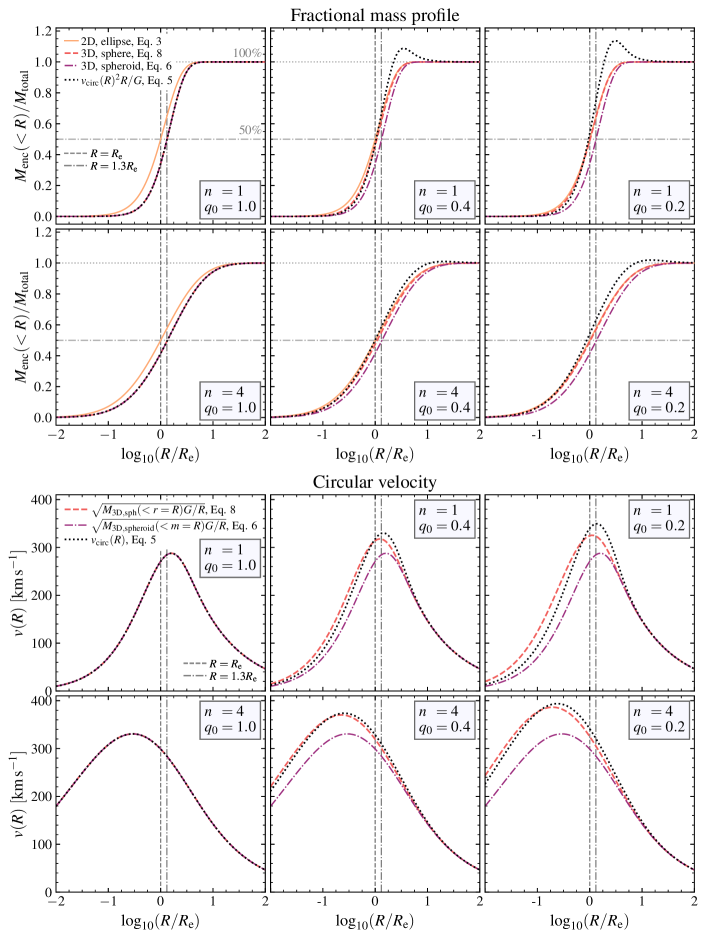
Figure 3: Example fractional enclosed mass (top) and circular velocity (bottom) profiles computed or inferred under different assumptions. The top and bottom rows show the profiles for Sérsic indices $n=1,4$, respectively, while the columns show intrinsic axis ratios $q_{0}=1,0.4,0.2$ (from left to right). For the top panels, we show the edge-on 2D projected mass enclosed within ellipses of axis ratio $q_{0}$ (orange solid line), the 3D mass profile enclosed within a sphere (red dashed line), the 3D mass profile enclosed within ellipsoids of intrinsic axis ratio $q_{0}$ (purple dashed dotted line), and the mass profile inferred from the flattened deprojected Sérsic model circular velocity under the simplifying assumption of spherical symmetry (i.e., $q_{0}=1$; black dotted line). In the bottom panels, we then compare the flattened deprojected Sérsic model circular velocity (black dotted line) to the inferred velocity profiles computed from the 3D spherical (red solid line) and the 3D ellipsoidal (purple dashed dotted) mass profiles under the simple assumption of spherical symmetry. The same total mass $M_{\mathrm{tot}}=5\times 10^{10}M_{\odot}$ is used for all cases. The vertical lines denote $R=R_{\mathrm{e}}$ (grey dashed) and $R=1.3R_{\mathrm{e}}$ ($\approx r_{1/2,\mathrm{mass,3D}}$ for $q_{0}=1$; grey dashed dotted). These enclosed mass and velocity profiles demonstrate that when $q_{0}\neq 1$, $M_{\mathrm{sph}}(<r=R)\neq v_{\mathrm{circ}}(R)^{2}R/G$. The non-spherical potentials for $q_{0}<1$ even result in $(v_{\mathrm{circ}}(R)^{2}R/G)/M_{\mathrm{tot}}>1$ between $R\sim 1-10R_{\mathrm{e}}$ (i.e., potentially leading to $\gtrsim 15\%$ overestimates in the system mass). We also see that as $q_{0}$ decreases, $M_{\mathrm{sph}}$ approaches the 2D projected mass profile, as the mass enclosed in a sphere versus an infinite ellipsoidal cylinder are equivalent for infinitely thin mass distributions.

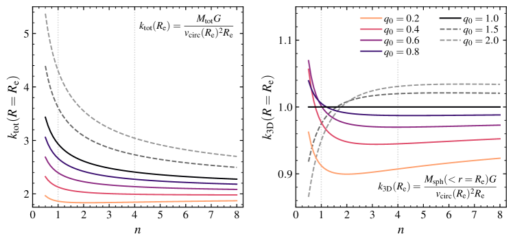
Figure 4: The total $k_{\mathrm{tot}}(R_{\mathrm{e}})$ (left) and 3D enclosed $k_{\mathrm{3D}}(R_{\mathrm{e}})$ (right) virial coefficients as a function of Sérsic index $n$ and intrinsic axis ratio $q_{0}$. The solid lines denote $q_{0}=0.2$ (orange) to $q_{0}=1$ (black), and two prolate cases are shown with dashed lines ($q_{0}=1.5,2$ in dark, light grey, respectively).

Table 2: Virial coefficients for select profiles and radii

		$k_{\mathrm{tot}}(R)$		$k_{\mathrm{3D}}(R)$
Sérsic index	Axis ratio	$R=R_{\mathrm{e}}$	$1.3\,R_{\mathrm{e}}$	$R=R_{\mathrm{e}}$	$1.3\,R_{\mathrm{e}}$
$n=1$	$q_{0}=0.4$	2.128	1.512	0.977	0.929
	$q_{0}=1\ \ \$	2.933	2.026	1	1
${}_{\,{}_{\,{}_{\,}}}$	$q_{0}=$ 1.5	3.613	2.459	0.975	0.995
$n=4$	$q_{0}=0.4$	1.993	1.707	0.945	0.941
	$q_{0}=1\ \ \$	2.408	2.033	1	1
${}_{\,{}_{\,{}_{\,}}}$	$q_{0}=$ 1.5	2.731	2.286	1.020	1.023

2.4 Properties of enclosed mass and circular velocity curves for non-spherical deprojected Sérsic profiles

The 3D spherical enclosed mass profiles for models with a range of Sérsic indices ($n=0.5,1,\ldots,8$) and different intrinsic axis ratios $q_{0}=1,0.4,0.2$) are shown in Figure 1. The 3D spherical half-mass radius (where $r_{1/2,\mathrm{mass,3D}}$ satisfies $M_{\mathrm{sph}}(<r_{1/2,\mathrm{mass,3D}})=M_{\mathrm{tot}}/2$) is $r_{1/2,\mathrm{mass,3D}}\sim 1.3R_{\mathrm{e}}$ when $q_{0}=1$ (as shown by Ciotti 1991). However, from the $q_{0}=0.2,0.4$ enclosed mass profiles, we see that the ratio $r_{1/2,\mathrm{mass,3D}}/R_{\mathrm{e}}$ varies with the model intrinsic axis ratio.

We quantify the dependence of the ratio between the 3D spherical half-mass radius and the projected effective radius, $r_{1/2,\mathrm{mass,3D}}/R_{\mathrm{e}}$, in Figure 2, as a function of Sérsic index, $n$, and intrinsic axis ratio, $q_{0}$. van de Ven & van der Wel 2021 make a similar comparison for both axisymmetric and triaxial systems using an approximation for $\rho$, but show $r_{1/2,\mathrm{mass,3D}}$ relative to the projected major axis, so for the axisymmetric, prolate systems our ratio differs from theirs. The 3D spherical half-mass radius is larger than the 2D projected effective radius enclosing half of the total light (and half of the total mass, assuming constant $M/L$ and an optically thin medium). There is a larger dependence of the ratio $r_{1/2,\mathrm{mass,3D}}/R_{\mathrm{e}}$ on $q_{0}$ than on $n$, where $r_{1/2,\mathrm{mass,3D}}/R_{\mathrm{e}}\sim 1.3-1.36$ when $q_{0}=1$ for all $n=0.5-8$, but as $q_{0}$ decreases the ratio decreases towards $r_{1/2,\mathrm{mass,3D}}/R_{\mathrm{e}}\sim 1$ for all $n$.

Next, we examine how the relation between the mass and circular velocity profiles deviates from the relation that holds for spherical symmetry, where $M_{\mathrm{sph}}(<r=R)=v_{\mathrm{circ}}^{2}(R)R/G$. In Figure 3 we show computed fractional enclosed mass (top) and circular velocity profiles (bottom) for $n=1,4$ (top and bottom rows, respectively) and for $q_{0}=1,0.4,0.2$ (left, center, right columns, respectively).

For the spherically symmetric ($q_{0}=1$) cases, the numerical evaluation of $M_{\mathrm{sph}}(<r=R)$ (red dashed line; Eq. 8) and $v_{\mathrm{circ}}(R)$ (black dotted line; Eq. 5) follow the expected relation ($M_{\mathrm{sph}}(<r=R)=v_{\mathrm{circ}}^{2}(R)R/G$), and the isodensity spheroids are spherical, so there is no difference between the enclosed spherical and spheroidal profiles. Echoing the previous figures, we also see that the enclosed 3D mass profile increases more slowly as a function of $R$ than the 2D projected profile (solid orange line; Eq. 3).

In contrast, for flattened deprojected models with $q_{0}<1$, the deviation of the $M_{\mathrm{sph}}(<r=R)$ and $v_{\mathrm{circ}}(R)$ profiles from the spherical relation become more pronounced for lower intrinsic axis ratios. Also, $\sqrt{M_{\mathrm{spheroid}}(<m=R)G/R}$ (purple dashed-dotted line; Eq. 6) does not match the correct $v_{\mathrm{circ}}(R)$ curve. As $q_{0}$ decreases, $M_{\mathrm{sph}}(<r=R)$ approaches the projected 2D ellipse curve, because for flatter deprojected models there is less additional mass outside the sphere along the remaining line-of-sight collapse.

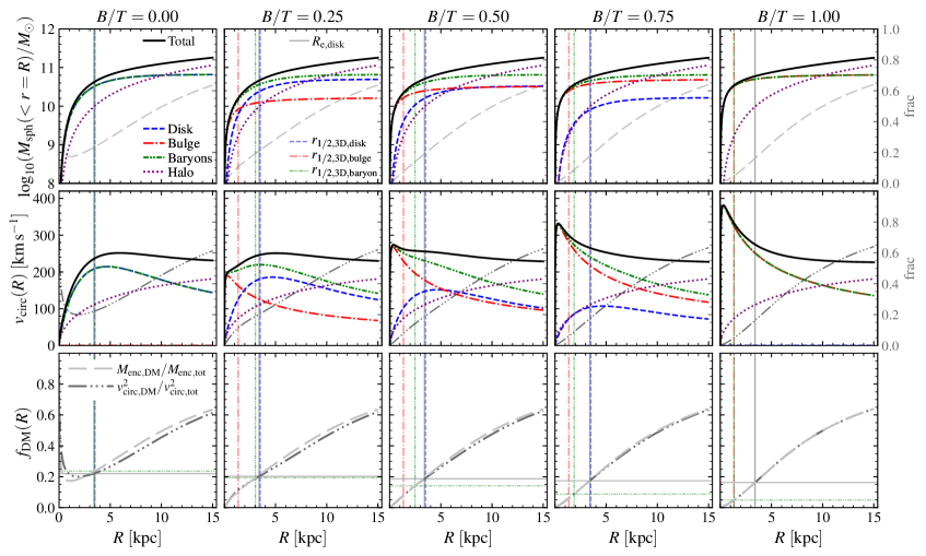
Figure 5: Enclosed mass (3D spherical, top), circular velocity (middle), and dark matter (bottom) profiles for different components of an example galaxy as a function of projected major axis radius, for bulge-to-total ratios of $B/T=0,0.25,0.5,0.75,1$ (left to right). For all cases, we compute the mass components assuming values for a typical $z=2$ massive main-sequence galaxy with $\log_{10}(M_{*}/M_{\odot})=10.5$: $M_{\mathrm{bar}}=6.6\times 10^{10}M_{\odot}$, $R_{\mathrm{e,disk}}=3.4\,\mathrm{\,kpc}$, $n_{\mathrm{disk}}=1$, $q_{0,\mathrm{disk}}=0.25$, $R_{\mathrm{e,bulge}}=1\,\mathrm{\,kpc}$, $n_{\mathrm{bulge}}=4$, $q_{0,\mathrm{bulge}}=1$, and a NFW halo with $M_{\mathrm{halo}}=8.9\times 10^{11}M_{\odot}$ and $c=4.2$. Shown are the $M_{\mathrm{sph}}(<r=R)$ and $v_{\mathrm{circ}}(R)$ profiles for the disk (dashed blue), bulge (dash-dot red), total baryons (disk+bulge; dash-dot-dot green), halo (dotted purple), and composite total system (solid black). Vertical lines mark $R=R_{\mathrm{e,disk}}$ (solid grey) and the 3D spherical half-mass radii $r_{1/2,\mathrm{mass,3D}}$ for the disk (dashed blue), bulge (dash-dot red), and total baryons (dash-dot-dot green). Two dark matter fraction definitions are shown in the bottom panels, $f_{\mathrm{DM}}^{m}=M_{\mathrm{DM,sph}}/M_{\mathrm{tot,sph}}$ and $f_{\mathrm{DM}}^{v}=v_{\mathrm{circ,DM}}^{2}/v_{\mathrm{circ,tot}}^{2}$, with long dashed grey and long dash-triple-dotted dark grey lines, respectively. (The $f_{\mathrm{DM}}^{m}$ and $f_{\mathrm{DM}}^{v}$ curves are also shown in the top and middle panels, respectively, with the scale at the right axis of each panel.) When a disk component is present, the system is no longer spherically symmetric, so $M_{\mathrm{DM,sph}}/M_{\mathrm{tot,sph}}$ and $v_{\mathrm{circ,DM}}^{2}/v_{\mathrm{circ,tot}}^{2}$ differ. This deviation is larger when the disk contribution is large (i.e., lower $B/T$), though even at low $B/T$ the difference is relatively modest (see also Figure 6). Additionally, while the ratio $r_{1/2,\mathrm{mass,3D}}/R_{\mathrm{e}}$ for a single component (e.g., the disk or bulge) is generally modest (see Figure 2), for a composite disk+bulge system the total baryon $r_{\mathrm{1/2,3D,baryon}}$ becomes much smaller relative to $R_{\mathrm{e,disk}}$ with increasing $B/T$ (vertical green dash-dot-dot and solid grey lines). If such disparate “half” radii definitions are used to define $f_{\mathrm{DM}}$ apertures (i.e., $f_{\mathrm{DM}}^{v}(R_{\mathrm{e,disk}})$ versus $f_{\mathrm{DM}}^{m}(r_{\mathrm{1/2,3D,baryon}})$, horizontal solid grey and green dash-dot-dot lines), this leads to increasingly large offsets between the $f_{\mathrm{DM}}$ values towards higher $B/T$ (see also Figure 7).

3 Virial coefficients for enclosed 3D and total masses

We now quantify the relationship between mass- and velocity-derived quantities for different Sérsic indices and intrinsic axis ratios. By including a “virial” coefficient $k_{\mathrm{3D}}(R)$ which depends on the geometry and mass distribution (Binney & Tremaine 2008), the spherical enclosed mass and circular velocity can be related by

$$M_{\mathrm{sph}}(<r=R)=k_{\mathrm{3D}}(R)\frac{v_{\mathrm{circ}}^{2}(R)R}{G}.$$ (9)

This virial coefficient is evaluated by combining Eqs. 5 and 8.

For comparison with integrated galaxy quantities, it is also useful to define a “total” virial coefficient $k_{\mathrm{tot}}(R)$ which relates the total system mass to the circular velocity at a given radius:

$$M_{\mathrm{tot}}=k_{\mathrm{tot}}(R)\frac{v_{\mathrm{circ}}^{2}(R)R}{G}.$$ (10)

Figure 4 shows $k_{\mathrm{tot}}(R=R_{\mathrm{e}})$ and $k_{\mathrm{3D}}(R=R_{\mathrm{e}})$ versus Sérsic index $n$ for a range of $q_{0}$. For the spherical case ($q_{0}=1$), $k_{\mathrm{3D}}(R=R_{\mathrm{e}})=1$, as expected by spherical symmetry. However, as $R_{\mathrm{e}}<r_{1/2,\mathrm{mass,3D}}$ for spherical deprojected Sérsic models, $k_{\mathrm{tot}}(R=R_{\mathrm{e}},q_{0}=1)\neq 2$, but instead exceeds 2 for all $n$ (i.e., 2.933 when $n=1$). For oblate flattened Sérsic deprojected models (i.e., $q_{0}<1$), $k_{\mathrm{tot}}(R=R_{\mathrm{e}})$ is lower than the $q_{0}=1$ case for all $n$, while prolate cases ($q_{0}>1$) have larger $k_{\mathrm{tot}}(R=R_{\mathrm{e}})$. For $k_{\mathrm{3D}}(R=R_{\mathrm{e}})$ the trends are more complex, but for $n\gtrsim 2$ the oblate (prolate) models all have $k_{\mathrm{3D}}(R=R_{\mathrm{e}})<1$ ($>1$). For reference, we also present values of $k_{\mathrm{tot}}(R)$ and $k_{\mathrm{3D}}(R)$ for a range of $R$, $n$, and $q_{0}$ in Table $a$. These total virial coefficients in particular allow for a more precise comparison between the dynamical $M_{\mathrm{tot}}$ and projection-derived quantities, such as $M_{*}$ or $M_{\mathrm{gas}}$, particularly when full dynamical modeling is not possible (e.g., the approach used in Erb et al. 2006, Miller et al. 2011, Price et al. 2016, 2020, and numerous other studies).

4 Mass distributions of multi-component galactic systems

4.1 Mass and velocity distributions of systems including both flattened and spherical components

While the virial coefficients derived in the previous section allow for the conversion from circular velocities to enclosed masses for a single non-spherical mass component, observed galaxies tend to have multiple mass components, of varying intrinsic shapes and profiles. We now explore the enclosed mass and circular velocity distributions for galaxies with multiple mass components, focusing on how the non-spherical components impact the mass fraction distributions inferred from velocity profile ratios.

We calculate profiles for a “typical” $z=2$ main-sequence star-forming galaxy of stellar mass $\log_{10}(M_{*}/M_{\odot})=10.5$ consisting of a bulge, disk, and halo, over a range of bulge-to-total ratios, $B/T$. We thus adopt a total $M_{\mathrm{bar}}=6.6\times 10^{10}M_{\odot}$ (using the gas fraction scaling relation of Tacconi et al. 2020). We assume a thick, flattened disk modeled as a deprojected Sérsic distribution with $q_{0,\mathrm{disk}}=0.25$, and adopt $n_{\mathrm{disk}}=1$, $R_{\mathrm{e,disk}}=3.4\mathrm{\,kpc}$ (from observed trends and scaling relations; Wuyts et al. 2011, van der Wel et al. 2014). The bulge is modeled as a deprojected Sérsic component with $n_{\mathrm{bulge}}=4$, $R_{\mathrm{e,bulge}}=1\mathrm{\,kpc}$, and $q_{0,\mathrm{bulge}}=1$. We also include a NFW halo without adiabatic contraction, assuming $\mathrm{conc}_{\mathrm{halo}}=4.2$ and $M_{\mathrm{halo}}=8.9\times 10^{11}M_{\odot}$ (following observed halo concentration and stellar mass to halo mass relations, e.g. Dutton & Macciò 2014, Moster et al. 2018). In Figure 5, for each of the $B/T$ ratios (left to right), we show the enclosed mass (top row) and circular velocity profiles (middle row) as a function of radius. The impact of shifting the baryonic mass from entirely in the disk (the only oblate, non-spherical mass component; $B/T=0$) to entirely in the bulge (only spherical mass components; $B/T=1$) can be seen in both the $M_{\mathrm{sph}}$ and $v_{\mathrm{circ}}$ profiles. The lower Sérsic index and larger $R_{\mathrm{e}}$ of the disk (blue dashed line) relative to the bulge (red dash-dot) result in more slowly rising mass and $v_{\mathrm{circ}}$ curves for the baryonic component (green dash-dot-dot) at low $B/T$, with the curves rising more quickly as the bulge contribution increases. The total galaxy mass and $v_{\mathrm{circ}}$ curves (solid black) are dominated by the baryonic components in the inner regions, but at large radii ($R\gtrsim 10\mathrm{\,kpc}$) where the halo begins dominating the mass and $v_{\mathrm{circ}}$ profiles, the curves are similar for all $B/T$.

We also show the radial variation of the 3D enclosed halo to total mass ratio $M_{\mathrm{DM,sph}}/M_{\mathrm{tot,sph}}$ (long light grey dashed line) and the squared halo to total circular velocity ratio $v_{\mathrm{circ,DM}}^{2}/v_{\mathrm{circ,tot}}^{2}$ (dark grey dash-triple dot line) in the bottom row (and the $M_{\mathrm{sph}}$ and $v_{\mathrm{circ}}$ panels, respectively). As expected when $B/T<1$, these two ratios are not equivalent, though they become closer as $B/T\to 1$ and more of the total galaxy mass is found in spherical components. For $B/T=1$, the galaxy is spherically symmetric, so the two ratios are equal.

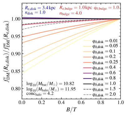
Figure 6: Ratio between the dark matter fraction at $R_{\mathrm{e,disk}}$ calculated from the circular velocity and from the 3D spherical enclosed mass, $f_{\mathrm{DM}}^{v}(R_{\mathrm{e,disk}})/f_{\mathrm{DM}}^{m}(R_{\mathrm{e,disk}})$, versus bulge-to-disk ratio $B/T$, for a range of different disk intrinsic axis ratios (colored lines, from $q_{0,\mathrm{disk}}=0.01$ to 1) for an example massive galaxy at $z=2$. The ratio between the two dark matter fraction measurements is lower for lower $B/T$ (i.e., higher disk contributions) and lower $q_{0,\mathrm{disk}}$ (i.e., more flattened disks), with $f_{\mathrm{DM}}^{v}(R_{\mathrm{e,disk}})/f_{\mathrm{DM}}^{m}(R_{\mathrm{e,disk}})\lesssim 0.9$ for low values of both $q_{0,\mathrm{disk}}$ and $B/T$. The limiting case of a Freeman (infinitely thin) exponential disk has $f_{\mathrm{DM}}^{v}(R_{\mathrm{e,disk}})/f_{\mathrm{DM}}^{m}(R_{\mathrm{e,disk}})\approx 0.84$. As $B/T$ increases for fixed $q_{0,\mathrm{disk}}$, and likewise for increasing $q_{0,\mathrm{disk}}$ at fixed $B/T$, the ratio of the two fraction measurements approaches 1 because the composite system becomes more spherical. Overall, the discrepancy between the $f_{\mathrm{DM}}$ estimators measured at the same radius is relatively minor.

4.2 Defining dark matter fractions

As illustrated in Figure 5, the approximation $v^{2}_{\mathrm{circ,DM}}(R)/v^{2}_{\mathrm{circ,tot}}(R)$ deviates from the enclosed spherical mass fraction $M_{\mathrm{DM,sph}}(<r=R)/M_{\mathrm{tot,sph}}(<r=R)$ for galaxies with a non-spherical disk component, particularly when the $B/T$ ratio is $\lesssim 0.5$. This deviation thus leads to differences in inferred dark matter fractions, depending on how the fraction is defined.

If the dark matter fraction is defined as the ratio of the dark matter to total mass enclosed within a sphere of a given radius, we have $f_{\mathrm{DM}}^{m}(R)=M_{\mathrm{DM,sph}}(<r=R)/M_{\mathrm{tot,sph}}(<r=R)$. This approach is often adopted for simulations, where it is easy to determine mass within a given radius. However, observations cannot directly probe the mass distributions, so generally the fraction is defined based on the circular velocity ratio, $f_{\mathrm{DM}}^{v}(R)=v_{\mathrm{circ,DM}}^{2}(R)/v_{\mathrm{circ,tot}}^{2}(R)$. If a galaxy has only spherically-symmetric components, these two definitions are equivalent (as seen in the right column of Figure 5), but as noted in Figure 5, the two definitions are no longer equivalent with non-spherical components, where $f_{\mathrm{DM}}^{m}$ is generally larger than $f_{\mathrm{DM}}^{v}$.

To further quantify how much these definitions can vary, we compare the value of the ratio between $f_{\mathrm{DM}}^{v}$ and $f_{\mathrm{DM}}^{m}$ at $R_{\mathrm{e,disk}}$ over a range of $B/T$ ratios and intrinsic disk thicknesses $q_{0,\mathrm{disk}}$ in Figure 6. For this example case (using a massive galaxy with $M_{\mathrm{bar}}=6.6\times 10^{10}M_{\odot}$ at $z=2$, as in Figure 5), we see that $f_{\mathrm{DM}}^{v}(R_{\mathrm{e,disk}})$ can be as low as $\sim 85\%$ of $f_{\mathrm{DM}}^{m}(R_{\mathrm{e,disk}})$ (in the extreme case with $q_{0,\mathrm{disk}}=0.01$). For more typical expected disk thicknesses for galaxies at $z\sim 1-3$, $q_{0,\mathrm{disk}}\sim 0.2-0.25$, we find a minimum of $f_{\mathrm{DM}}^{v}(R_{\mathrm{e,disk}})/f_{\mathrm{DM}}^{m}(R_{\mathrm{e,disk}})\sim 0.93-0.95$ (for $B/T=0$). While this deviation is fairly small in this example, using consistent definitions of $f_{\mathrm{DM}}$ when comparing simulations and observations would avoid introducing systematic shifts between the values.

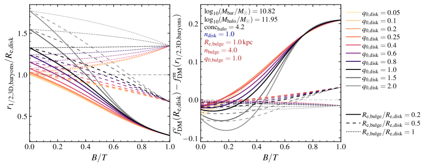
Figure 7: Ratio between the composite disk+bulge 3D half-mass radius and the 2D projected disk effective radius ($r_{1/2,\mathrm{3D,baryons}}/R_{\mathrm{e,disk}}$; left) and the difference between the dark matter fraction estimators at these radii ($f_{\mathrm{DM}}^{v}(R_{\mathrm{e,disk}})-f_{\mathrm{DM}}^{m}(r_{1/2,\mathrm{3D,baryons}})$; right), as a function of $B/T$, for a range of disk intrinsic axis ratios (colored lines, from $q_{0,\mathrm{disk}}=0.05$ to 2) and ratio between the bulge and disk $R_{\mathrm{e}}$ (solid, dashed, and dotted lines, for $R_{\mathrm{e,bulge}}/R_{\mathrm{e,disk}}=0.2,0.5,1$, respectively). The adopted galaxy values are the same as in Figure 6, except $R_{\mathrm{e,disk}}$ is now determined by $R_{\mathrm{e,bulge}}/R_{\mathrm{e,disk}}$. With a non-zero bulge contribution, $r_{1/2,\mathrm{3D,baryons}}/R_{\mathrm{e,disk}}$ deviates from the single-component ratio (Figure 2), decreasing with increasing $B/T$ for $R_{\mathrm{e,disk}}=2,5\mathrm{\,kpc}$ for all $q_{0,\mathrm{disk}}$ (though increasing with $B/T$ when $q_{0}<1,R_{\mathrm{e,disk}}=R_{\mathrm{e,bulge}}=1\mathrm{\,kpc}$). For large $B/T$ and $R_{\mathrm{e,disk}}=5\mathrm{\,kpc}$, the composite $r_{1/2,\mathrm{3D,baryons}}$ is less than 50% of $R_{\mathrm{e,disk}}$. If the dark matter fractions are measured at different radii, the mismatch of the aperture sizes will lead to much larger $f_{\mathrm{DM}}$ differences than those found for the simple estimator mismatch ($f_{\mathrm{DM}}^{m}$ vs $f_{\mathrm{DM}}^{v}$ at the same radius; Figure 6). Here, we have shown $f_{\mathrm{DM}}^{v}(R_{\mathrm{e,disk}})$, as might be adopted for modeling of observations, and $f_{\mathrm{DM}}^{m}(r_{1/2,\mathrm{3D,baryons}})$, representing a simple option for simulations (where spherical curves of growth separating gas, star, and DM particles could be used to find both the composite baryon $r_{1/2,\mathrm{3D,baryons}}$ within, e.g., $R_{\mathrm{vir}}$ and then $f_{\mathrm{DM}}^{m}$). For small $B/T$, $f_{\mathrm{DM}}^{m}(r_{1/2,\mathrm{3D,baryons}})$ is larger than $f_{\mathrm{DM}}^{v}(R_{\mathrm{e,disk}})$, but for large $B/T$, the trend reverses (excepting the $R_{\mathrm{e,disk}}=R_{\mathrm{e,bulge}}=1\mathrm{\,kpc}$ case), and $f_{\mathrm{DM}}^{v}(R_{\mathrm{e,disk}})$ can be up to 50%-400% larger than $f_{\mathrm{DM}}^{m}(r_{1/2,\mathrm{3D,baryons}})$ as $B/T\to 1$ (for $R_{\mathrm{e,disk}}=2,5\mathrm{\,kpc}$, respectively). This example illustrates how, depending on galaxy structures, quoted “half-mass” $f_{\mathrm{DM}}$ values can be very different — but that this is primarily driven by the aperture radii definitions and not by estimator mismatches.

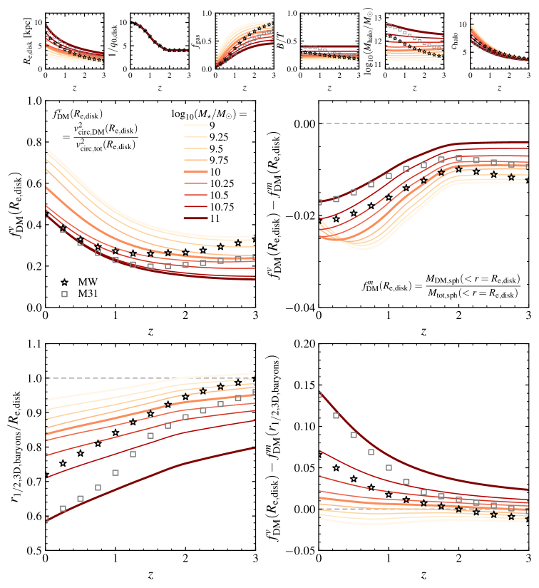
Figure 8: Toy model of how $f_{\mathrm{DM}}^{v}(R_{\mathrm{e,disk}})$ (upper left), $f_{\mathrm{DM}}^{v}(R_{\mathrm{e,disk}})-f_{\mathrm{DM}}^{m}(R_{\mathrm{e,disk}})$ (upper right), $r_{1/2,\mathrm{3D,baryons}}/R_{\mathrm{e,disk}}$ (lower left), and $f_{\mathrm{DM}}^{v}(R_{\mathrm{e,disk}})-f_{\mathrm{DM}}^{m}(r_{1/2,\mathrm{3D,baryons}})$ (lower right) vary with redshift for a range of fixed $\log_{10}(M_{*}/M_{\odot})$, using “typical” galaxy sizes, intrinsic axis ratios, gas fractions, $B/T$ ratios, halo masses, and halo concentrations (from empirical scaling relations or other estimates; Dutton & Macciò 2014, Lang et al. 2014, van der Wel et al. 2014, Moster et al. 2018, Übler et al. 2019, Tacconi et al. 2020, Genzel et al. 2020). The assumed (interpolated, extrapolated) property profiles as a function of redshift for each of the fixed $\log_{10}(M_{*}/M_{\odot})$ are shown in the top panels. Using abundance-matching models (inferred from Fig. 4 of Papovich et al. 2015, based on the models of Moster et al. 2013), we show the path of a Milky Way (MW, $M_{*}=5\times 10^{10}M_{\odot}$ at $z=0$; black stars) and M31 progenitor ($M_{*}=10^{11}M_{\odot}$ at $z=0$; grey squares) over time in each of the panels, assuming the progenitors are “typical” at all times. This inferred “typical” evolution would predict an increase in $f_{\mathrm{DM}}(R_{\mathrm{e,disk}})$ with time at fixed $M_{*}$, with lower masses having higher $f_{\mathrm{DM}}$ at all $z$. The evolution of the structure and relative masses of the disk, bulge, and halo predict an increase ($M_{*}\gtrsim 10^{10.25}M_{\odot}$) or “dip” ($M_{*}\lesssim^{10.25}M_{\odot}$) in the difference $f_{\mathrm{DM}}^{v}(R_{\mathrm{e,disk}})-f_{\mathrm{DM}}^{m}(R_{\mathrm{e,disk}})$ between $z\sim 0$ and $z\sim 0.75$, and then an increase until $z\sim 2$ when the difference flattens (largely reflecting the flat $q_{0,\mathrm{disk}}$ estimate for $z\gtrsim 2$). The difference is minor, between $\sim-0.025$ and $-0.005$ for the stellar masses shown. The ratio of the composite $r_{1/2,\mathrm{3D,baryons}}/R_{\mathrm{e,disk}}$ increases with redshift for all masses, with more massive models predicting smaller ratios at each $z$. The MW and M31 progenitors have $f_{\mathrm{DM}}(R_{\mathrm{e,disk}})$ evolving from $\sim 0.33$ and $\sim 0.25$ (respectively) at $z=3$, decreasing to $\sim 0.25$ and $\sim 0.2$ at $z\sim 1.5$, and then increasing to roughly same value $\sim 0.45$ at $z=0$. The $f_{\mathrm{DM}}^{v}(R_{\mathrm{e,disk}})$ and $f_{\mathrm{DM}}^{m}(r_{1/2,\mathrm{3D,baryons}})$ values are relatively similar down to $z\sim 1.5$, but at lower redshifts (where $r_{1/2,\mathrm{3D,baryons}}/R_{\mathrm{e,disk}}\lesssim 0.9$) the difference increases up to $\sim 0.065$ (MW) and $\sim 0.14$ (M31) at $z\sim 0$. While this “typical” case predicts $f_{\mathrm{DM}}$ offsets of only 0.035 at $z=2$ and increasing to 0.14 at $z\sim 0$ for the most massive case, objects with even larger bulges ($B/T>0.4$) or radii above the mass-size relation will have even more discrepant $f_{\mathrm{DM}}$ values when adopting these radii definitions (see Figure 7).

4.3 Impact of aperture effects on dark matter fractions

While the fractional differences between the 3D half mass radii $r_{1/2,\mathrm{mass,3D}}$ and the projected 2D effective radii $R_{\mathrm{e}}$ for a single component, and between the $f_{\mathrm{DM}}^{v}$ and $f_{\mathrm{DM}}^{m}$ definitions are generally small for expected galaxy thicknesses, measuring $f_{\mathrm{DM}}$ (of either indicator) at different radii — such as the easily measurable $r_{1/2,\mathrm{mass,3D}}$ for simulations versus $R_{\mathrm{e}}$ for observations — can lead to very large discrepancies in the $f_{\mathrm{DM}}$ values. We demonstrate this issue in Figure 7.

First, while we show the ratio of $r_{1/2,\mathrm{mass,3D}}$/$R_{\mathrm{e}}$ for a single component in Figure 2, the ratio for a multi-component system is not self-similar, but depends also on the ratio of effective radii for the components. For a disk + bulge system, a number of observational studies use the disk effective radius as the dark matter fraction aperture. We thus determine the 3D half-mass radius for the composite disk+bulge system, and plot the ratio $r_{1/2,\mathrm{3D,baryons}}$/$R_{\mathrm{e,disk}}$ as a function of $B/T$ in the left panel of Figure 7, for a range of ratios $R_{\mathrm{e,bulge}}$/$R_{\mathrm{e,disk}}$ (line style) and disk intrinsic thicknesses ($q_{0,\mathrm{disk}}$, assuming a spherical bulge). Depending on the $R_{\mathrm{e,bulge}}$/$R_{\mathrm{e,disk}}$ and $q_{0,\mathrm{disk}}$ values, this ratio can range from $\sim 0.3-1.3$ (for oblate or spherical disk geometries, or up to $\sim 1.7$ for prolate disks), with the lowest values arising from the combination of a low $R_{\mathrm{e,bulge}}$/$R_{\mathrm{e,disk}}$ and a high $B/T$.

We then demonstrate the effects of measuring $f_{\mathrm{DM}}$ at these different aperture radii in the right panel of Figure 7. Here we plot the absolute difference $f_{\mathrm{DM}}^{v}(R_{\mathrm{e,disk}})-f_{\mathrm{DM}}^{m}(r_{1/2,\mathrm{3D,baryons}})$ as a function of $B/T$, calculated for the same $R_{\mathrm{e,bulge}}$/$R_{\mathrm{e,disk}}$ and $q_{0,\mathrm{disk}}$ values. For consistency, the $f_{\mathrm{DM}}$ estimators for each are chosen to reflect the typical definitions from observations and simulations, respectively, in line with the “half-mass” radii choices (though, as seen in Figure 6, using $f_{\mathrm{DM}}^{v}$ versus $f_{\mathrm{DM}}^{m}$ contributes very little to the differences seen in this figure). For very low $B/T$, most cases produce $f_{\mathrm{DM}}^{v}(R_{\mathrm{e,disk}})-f_{\mathrm{DM}}^{m}(r_{1/2,\mathrm{3D,baryons}})\sim-0.025$ (e.g., larger $f_{\mathrm{DM}}^{m}(r_{1/2,\mathrm{3D,baryons}})$). For most practical cases with a larger disk than bulge ($R_{\mathrm{e,bulge}}/R_{\mathrm{e,disk}}<1$), the difference increases towards larger $B/T$, with $f_{\mathrm{DM}}^{v}(R_{\mathrm{e,disk}})>f_{\mathrm{DM}}^{m}(r_{1/2,\mathrm{3D,baryons}})$ by $B/T\sim 0.2-0.5$ (for $R_{\mathrm{e,bulge}}/R_{\mathrm{e,disk}}=0.2,0.5$, respectively). This difference can be very large, up to $\sim 0.2$ for large $B/T$ and low $R_{\mathrm{e,bulge}}/R_{\mathrm{e,disk}}$, as might be expected for massive galaxies that simultaneously have massive bulges (i.e., high $B/T$) but also large disk effective radii (i.e., low $R_{\mathrm{e,bulge}}$/$R_{\mathrm{e,disk}}$).

We extend these test cases to consider how $f_{\mathrm{DM}}$ for the different definitions and apertures change with redshift and stellar mass for a “typical” star-forming galaxy, as shown in Figure 8. We use empirical scaling relations or other estimates to determine $R_{\mathrm{e,disk}}$, $q_{0,\mathrm{disk}}$, $f_{\mathrm{gas}}$, $B/T$, $\log_{10}(M_{\mathrm{halo}}/M_{\odot})$, and $c_{\mathrm{halo}}$ for a range of $z$ and $\log_{10}(M_{*}/M_{\odot})$ (assuming the disk and bulge follow deprojected Sérsic models, with fixed $n_{\mathrm{disk}}=1$, $n_{\mathrm{bulge}}=4$, and $R_{\mathrm{e,bulge}}=1\mathrm{\,kpc}$; top panels). These toy models predict $f_{\mathrm{DM}}^{v}(R_{\mathrm{e}})$ (Figure 8, center left) to increase over time at fixed stellar mass (in part because of the increasing $c_{\mathrm{halo}}$ and $R_{\mathrm{e,disk}}$ over time), and that lower $M_{*}$ galaxies have higher $f_{\mathrm{DM}}^{v}(R_{\mathrm{e}})$ at fixed redshift, with relatively low $f_{\mathrm{DM}}^{v}(R_{\mathrm{e}})$ for the most massive galaxies ($\sim 20\%$) at $z\sim 1-3$. This is qualitatively in agreement with recent observations (e.g., Genzel et al. 2020, Price et al. 2021, Bouché et al. 2022), though these recent studies also provide evidence for non-NFW halo profiles (in particular, cored profiles), which would produce lower $f_{\mathrm{DM}}^{v}(R_{\mathrm{e}})$ for the same $M_{\mathrm{halo}}$ than our toy models. As a further example, we consider how the predictions would change over time for a Milky Way and M31-mass progenitor. In both cases, the predicted $f_{\mathrm{DM}}^{v}(R_{\mathrm{e}})$ decrease from $z=3$ to a minimum at $z\sim 1.5$, and then increase until the present day. For these toy values, the difference in dark matter fraction definitions measured at the same radius ($R_{\mathrm{e,disk}}$; Figure 8, center right) typically differ by only $\sim-0.005$ to $\sim-0.025$ (typically $\sim 4-6\%$ of the measured values), with a larger typical offset at lower redshifts and for lower masses.

We find the ratio of the 3D baryonic half mass radius to the disk effective radius ($r_{1/2,\mathrm{3D,baryons}}/R_{\mathrm{e,disk}}$; Figure 8, bottom left) for these models decreases towards lower redshifts and with increasing stellar mass, from $\sim 1$ at $z\sim 2-3$ to $\sim 0.94$ at $z=0$ for the lowest $M_{*}$, and from $\sim 0.8$ at $z=3$ down to $\sim 0.6$ at $z=0$ for the highest $M_{*}$. For the MW and M31 progenitors, this ratio decreases from $\sim 1,0.96$ at $z=3$ down to $\sim 0.72,0.59$ at $z=0$, respectively. The difference between the two dark matter fraction definitions measured at these different radii apertures ($f_{\mathrm{DM}}^{v}(R_{\mathrm{e,disk}})-f_{\mathrm{DM}}^{m}(r_{1/2,\mathrm{3D,baryons}})$; Figure 8, bottom right) for these toy models is typically much larger than the difference for the definitions alone, and tends to increase towards lower redshifts and with stellar mass. The difference changes from $\sim-0.015,0.,0.025$ at $z=3$ to $\sim-0.01,0.015,0.14$ at $z=0$ for $\log_{10}(M_{*}/M_{\odot})=9,10,11$, respectively. The MW and M31 progenitors have offsets increasing from $\sim-0.013,-0.003$ at $z=3$ to $\sim 0.065,0.14$ at $z=0$, respectively.

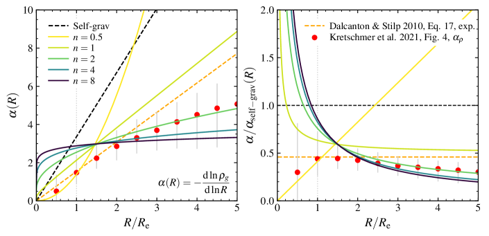
Figure 9: The pressure support correction, $\alpha(R)$, versus $R/R_{\mathrm{e}}$ for a self-gravitating exponential disk and deprojected Sérsic models. The left panel directly compares $\alpha_{\mathrm{self-grav}}(r)=3.36(R/R_{\mathrm{e}})$ for the self-gravitating disk (as in Burkert et al. 2010; black dashed line) to $\alpha(R,n)=-\mathrm{d}\ln\rho(R,n)/\mathrm{d}\ln R$ determined for a range of Sérsic indices $n$ (colored lines). The ratio $\alpha/\alpha_{\mathrm{self-grav}}(R)$ is shown in the right panel. For $n\geq 1$, $\alpha(n)$ is smaller than $\alpha_{\mathrm{self-grav}}$ when $R\gtrsim 0.2-0.8R_{\mathrm{e}}$, though $\alpha(n\geq 1)$ does exceed $\alpha_{\mathrm{self-grav}}$ at the smallest radii. This implies that for most radii, there is less asymmetric drift correction (and thus higher $v_{\mathrm{rot}}$) for the deprojected Sérsic models (e.g., $n=1$) than for the self-gravitating disk. However, for $n=0.5$, $\alpha(n)$ is greater than $\alpha_{\mathrm{self-grav}}$ at $R\gtrsim 2.4R_{\mathrm{e}}$, so at large radii the $n=0.5$ deprojected Sérsic model predicts a larger pressure support correction than for the self-gravitating disk case. The lower pressure support predicted for $\alpha(n\gtrsim 1)$ than for $\alpha_{\mathrm{self-grav}}$ is in agreement with recent predictions from simulations by Kretschmer et al. (2021) (red circles; with the vertical grey bars denoting the $1\sigma$ distribution), as well the relation by Dalcanton & Stilp (2010) for a power law relationship between the gas surface density and the turbulent pressure (orange dashed line).

      

      

      

      

Given the very modest offsets for the $f_{\mathrm{DM}}$ definition differences alone, these offsets are nearly entirely driven by the differences between the aperture radii. Indeed, though the differences for these toy calculations — driven almost entirely by the aperture mismatches — do not reach the extreme differences of $f_{\mathrm{DM}}^{v}(R_{\mathrm{e,disk}})-f_{\mathrm{DM}}^{m}(r_{1/2,\mathrm{3D,baryons}})$ seen in Figure 7 for parts of the parameter space (in part because the maximum toy model $B/T$ is $\sim 0.4$), we still predict absolute differences up to almost $\sim 0.15$ at $z=0$, and $\sim 0.03-0.07$ at $z\sim 1-2$. This offset is on par with the current observational uncertainties at $z\gtrsim 1$ ($\sim 0.1-0.2$; e.g., Genzel et al. 2020). To ensure the most direct comparison between observations and simulations — particularly as observational constraints on $f_{\mathrm{DM}}$ at higher redshifts continue to improve — it will be important to account for such aperture differences (either by measuring in equivalent apertures, or by applying an appropriate correction factor) in order to better determine if, and how, observation and simulation predictions differ.

5 Turbulent pressure support effects on rotation curves

5.1 Derivation of pressure support for a single component

As many dynamical studies of high-redshift, turbulent disk galaxies use gas motions as the dynamical tracer, we now consider how turbulent pressure support will modify the rotation curves if the gas is described by a deprojected Sérsic model. We follow the derivation of Burkert et al. (2010), and also assume the pressure support is due only to the turbulent gas motions (i.e., the thermal contribution is negligible). We thus begin from Eq. 2 of Burkert et al. (2010), where the pressure-corrected gas rotation velocity is

$$v_{\mathrm{rot}}^{2}(R)=v_{\mathrm{circ}}^{2}(R)+\frac{1}{\rho_{g}}\frac{\mathrm{d}}{\mathrm{d}\ln{}R}\left(\rho_{g}\sigma^{2}\right),$$ (11)

where $v_{\mathrm{circ}}$ is the circular velocity in the midplane of the galaxy determined from the total system potential (including all mass components: stars, gas, and halo; i.e., the rotational velocity if there is no pressure support), $\rho_{g}$ is the gas density, and $\sigma$ is the (one-dimensional) gas velocity dispersion. While the gas has the same circular velocity as the total system, the pressure support correction term from the turbulent gas motions only applies to the gas rotation and only depends on the gas density distribution and the gas velocity dispersion.

This relation can be generally rewritten as

$$v_{\mathrm{rot}}^{2}(R)=v_{\mathrm{circ}}^{2}(R)-\sigma^{2}\alpha(R),$$ (12)

where $\alpha(R)=-\Big{(}\frac{\mathrm{d}\ln\rho_{g}}{\mathrm{d}\ln{}R}+\frac{\mathrm{d}\ln\sigma^{2}}{\mathrm{d}\ln{}R}\Big{)}$. If we assume the velocity dispersion $\sigma=\sigma_{0}$ is constant, then this simplifies to

$$\alpha(R)=-\frac{\mathrm{d}\ln\rho_{g}}{\mathrm{d}\ln{}R}.$$ (13)

For a self-gravitating exponential disk, as assumed in Burkert et al. (2010), $\frac{\mathrm{d}\ln\rho_{g}}{\mathrm{d}\ln{}R}=2\left(\!\frac{\mathrm{d}\ln\Sigma(R)}{\mathrm{d}\ln{}R}\!\right)$, which yields

$$\alpha_{\mathrm{self-grav}}(R)=2(R/R_{d})=3.36(R/R_{\mathrm{e}}).$$ (14)

Burkert et al. (2016) generalized this result to a self-gravitating disk with an arbitrary Sérsic index, where $\alpha_{\mathrm{self-grav},n}(R)=2b_{\mathrm{n}}(R/R_{\mathrm{e}})^{1/n}$.

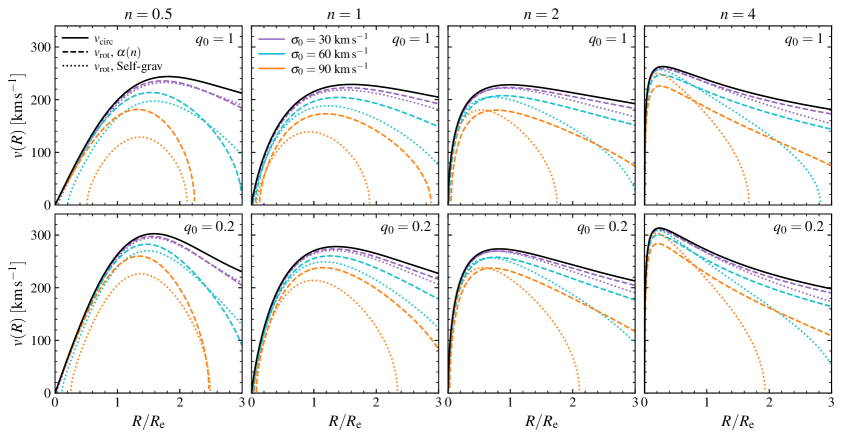
Figure 10: Comparison between $v_{\mathrm{rot}}^{2}=v_{\mathrm{circ}}^{2}-\sigma_{0}^{2}\alpha(R)$ determined using the deprojected Sérsic model $\alpha(n)$ and the self-gravitating exponential disk $\alpha_{\mathrm{self-grav}}$ (as shown in Figure 9), for a range of Sérsic indices $n$, intrinsic axis ratios $q_{0}$, and velocity dispersions $\sigma_{0}$. For all cases, we consider a single deprojected Sérsic mass distribution with $M_{\mathrm{tot}}=10^{10.5}\,M_{\odot}$. The columns show curves for $n=0.5,1,2,4$ (left to right, respectively), while the rows show the case of spherical ($q_{0}=1$; top) and flattened ($q_{0}=0.2$; bottom) Sérsic distributions. For each panel, the solid black line shows the circular velocity $v_{\mathrm{circ}}$ (determined following Eq. 5). The colored lines show $v_{\mathrm{rot}}$ determined using $\alpha(n)$ (dashed) and $\alpha_{\mathrm{self-grav}}$ (dotted), with the colors denoting $\sigma_{0}=[30,60,90]\mathrm{\,km\,s^{-1}}$ (purple, turquoise, orange, respectively). As expected by the $\alpha(R)$ trends shown in Figure 9, for $n\geq 1$ we see that for most radii, the pressure support implied by $\alpha_{\mathrm{self-grav}}$ results in lower $v_{\mathrm{rot}}$ than for $\alpha(n)$ (though at the smallest radii the inverse holds). In some cases, the magnitude of $\sigma_{0}$ combined with the form of $\alpha(R)$ additionally predict disk truncation within the range shown, though truncation generally occurs at smaller radii for $\alpha_{\mathrm{self-grav}}$ than for $\alpha(n)$.

Alternatively, as derived by Dalcanton & Stilp (2010) (their Eqs. 16 & 17), for a disk with turbulent pressure $P_{\mathrm{turb}}\propto\Sigma^{0.92}$ (where the authors infer the exponent using results from hydrodynamical simulations of turbulence in stratified gas by Joung et al. 2009 combined with a Schmidt law of slope $N=1.4$; Kennicutt 1998), the pressure support is described by

$$\alpha_{\mathrm{DS10}}(R) =-0.92\frac{\mathrm{d}\ln\Sigma(R)}{\mathrm{d}\ln{}R}=0.92\left(\frac{b_{\mathrm{n}}}{n}\right)\left(\frac{R}{R_{\mathrm{e}}}\right)^{1/n},$$ (15)

$$=1.5456(R/R_{\mathrm{e}})\qquad\mathrm{for}\ n=1,$$ (16)

for arbitrary $\sigma_{R}(R)$ (not only constant $\sigma_{0}$ as considered here). Further forms of the pressure support have also been explored, as compared and discussed by Bouché et al. (2022), including the case for constant disk thickness (Meurer et al. 1996, Bouché et al. 2022), or when accounting for the full Jeans equation (Weijmans et al. 2008).

For gas following a deprojected Sérsic model, we find $\alpha(R)=\alpha(R,n)$ by differentiating $\rho_{g}=\rho(m=R,n)$. After combining Equations 2 & 4, performing a change of variable, and applying the Leibniz rule, we can write

$$\frac{\mathrm{d}\rho(m)}{\mathrm{d}m} =\frac{\Upsilon}{\pi}\frac{q_{\mathrm{obs}}}{q_{0}}\frac{I_{e}b_{\mathrm{n}}}{nR_{\mathrm{e}}}\frac{m}{R_{\mathrm{e}}^{2}}\int_{0}^{\infty}f(m,x)\>\mathrm{d}x,$$ (17)

$$f(m,x) =\exp\left\{-b_{\mathrm{n}}\left[v^{1/n}-1\right]\right\}v^{\left(1/n-4\right)}\left[\frac{1}{n}-2-\frac{b_{\mathrm{n}}}{n}v^{1/n}\right],$$

$$\mathrm{for\ }v=\frac{1}{R_{\mathrm{e}}}\sqrt{x^{2}+m^{2}}.$$

This expression for $\mathrm{d}\rho(m)/\mathrm{d}{}m$ can be evaluated numerically, and together with the numerical evaluation of $\rho(m)$, we have $\mathrm{d}\ln\rho/\mathrm{d}\ln m=(m/\rho)(\mathrm{d}\rho/\mathrm{d}m)$. Alternatively, the log density can be differentiated numerically. (A similar derivation of the pressure support for spherical deprojected Sérsic profiles is presented in Sec. 2.2.3 of Kretschmer et al. 2021, who also showed $\alpha(n)$ versus $n$ at select radii in their Fig. 6, and gave an approximate equation for $\alpha(n)$ at select radii in Sec. 3.5).

Figure 9 (left panel) shows the $\alpha(R,n)$ derived for the deprojected Sérsic models as a function of radius for a range of Sérsic index $n$ (colored lines). For comparison, we also show the self-gravitating disk case $\alpha_{\mathrm{self-grav}}(R)$ as presented in Burkert et al. (2010) (black dashed line), as well as $\alpha$ determined following Dalcanton & Stilp (2010), and as measured from simulations in Kretschmer et al. (2021) (where the density is determined from the smoothed cumulative mass profile of the cold gas, and $R_{\mathrm{e}}$ of the cold gas is the half-mass radius measured within $0.1R_{\mathrm{vir}}$; c.f. Sec 2.3 & 3.2 of Kretschmer et al. 2021). The right panel additionally shows the ratio $\alpha/\alpha_{\mathrm{self-grav}}$. We find that $\alpha(n)$ is lower than $\alpha_{\mathrm{self-grav}}$ at $R\gtrsim 0.2-0.8R_{\mathrm{e}}$ for $n\gtrsim 1$. However, at small radii ($R\lesssim R_{\mathrm{e}}$) we find $\alpha(n)>\alpha_{\mathrm{self-grav}}$ for $n\gtrsim 1$ (with the cross-over radius varying with $n$). In contrast, we find the inverse for $n=0.5$: $\alpha(n=0.5)$ is lower than $\alpha_{\mathrm{self-grav}}$ up to $R\sim 2.4R_{\mathrm{e}}$, but then $\alpha(n)$ exceeds $\alpha_{\mathrm{self-grav}}$ at larger radii. In comparison to the self-gravitating disk case, we find the deprojected Sérsic $\alpha(n)$ are in better agreement with the pressure support for an exponential distribution from Dalcanton & Stilp (2010) (roughly half as much pressure support as the self-gravitating case), as well as with the simulation-derived pressure support by Kretschmer et al. (2021) (and similar findings by Wellons et al. 2020). Furthermore, as demonstrated by Bouché et al. (2022) (using an example $v_{\mathrm{circ}}$ with $n=1.5$ and an NFW profile), the Dalcanton & Stilp (2010) correction produces pressure support that is very similar to the constant scale height ($\rho(R)\propto\Sigma(R)$, Meurer et al. 1996, Bouché et al. 2022) and Weijmans et al. 2008 cases (assuming constant dispersion), which all predict lower support corrections than for the self-gravitating disk case. This difference arises because these three cases assume constant scale height or a thin disk approximation, resulting in a correction of approximately $\mathrm{d}\ln\Sigma(R)/\mathrm{d}\ln{}R$. In contrast, the self-gravitating disk case explicitly assumes a constant vertical dispersion, so predicts $\rho(R)\propto\Sigma(R)^{2}$, yielding a correction term that is roughly twice that of the other cases.

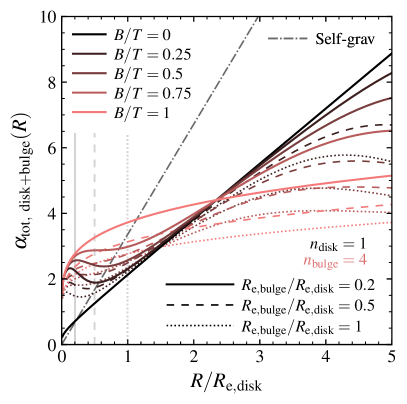
Figure 11: Composite pressure support correction, $\alpha_{\mathrm{tot}}(R)$, for gas distributed in a composite disk+bulge system (with $n_{\mathrm{disk}}=1$, $n_{\mathrm{bulge}}=4$), for a range of $B/T$ (colors) and $R_{\mathrm{e,bulge}}/R_{\mathrm{e,disk}}$ ratios (dash length). For the limiting cases, we recover the profiles shown in Figure 9: $B/T=0$ has $\alpha_{\mathrm{tot}}=\alpha(n=1)$ (black solid line), while $B/T=1$ has $\alpha_{\mathrm{tot}}=\alpha(n=4)$ but with different radial scaling, owing to the different adopted $R_{\mathrm{e,bulge}}/R_{\mathrm{e,disk}}$ ratios (colored lines). For the cases with $0<B/T<1$, the bulge contribution modifies the $\alpha(n=1)$ profile at both small and large radii, leading to larger $\alpha_{\mathrm{tot}}$ in inner regions and smaller $\alpha_{\mathrm{tot}}$ in the outskirts ($R/R_{\mathrm{e,disk}}\lesssim,\gtrsim 1-2$). At fixed $B/T$, the deviation from the disk $\alpha(n=1)$ in the center ($R/R_{\mathrm{e,disk}}\lesssim 1-2$) is larger for smaller $R_{\mathrm{e,bulge}}/R_{\mathrm{e,disk}}$, while at large radii the deviation is larger for larger $R_{\mathrm{e,bulge}}/R_{\mathrm{e,disk}}$. For reference, we mark $R_{\mathrm{e,bulge}}/R_{\mathrm{e,disk}}$ with vertical light grey lines, and also show $\alpha_{\mathrm{self-grav}}$ (grey dash-dot line).

These differences between $\alpha$ predict different pressure support-corrected $v_{\mathrm{rot}}(R)$ for the same circular velocity profile and intrinsic velocity dispersion. We demonstrate these differences for $\alpha$ for deprojected Sérsic models and a self-gravitating disk in Figure 10, over a range of Sérsic indices ($n=0.5,1,2,4$; left to right) and intrinsic axis ratios ($q_{0}=1,0.2$; top and bottom, respectively). For all cases, we determine the circular velocity $v_{\mathrm{circ}}$ (solid black line) assuming the mass distribution follows a single deprojected Sérsic model of $M_{\mathrm{tot}}=10^{10.5}M_{\odot}$ (i.e., a pure gas disk, or gas+stars where both components follow the same density distribution). We then calculate $v_{\mathrm{rot}}$ using both $\alpha(n)$ and $\alpha_{\mathrm{self-grav}}$ (dashed and dotted lines, respectively). As implied by Figure 9, for $n\gtrsim 1$ the rotation curves $v_{\mathrm{rot}}$ computed with $\alpha(n)$ are higher than with $\alpha_{\mathrm{self-grav}}$ at $R\gtrsim R_{\mathrm{e}}$ (i.e., smaller correction from $v_{\mathrm{circ}}$). The difference between the two $v_{\mathrm{rot}}$ curves becomes more pronounced towards larger radii, in line with the continued decrease of $\alpha(n)/\alpha_{\mathrm{self-grav}}$ with increasing radius. We also see the opposite behavior in the $n=0.5$ case, where $v_{\mathrm{rot}}$ computed in the self-gravitating case is higher than for $\alpha(n)$ at $R\gtrsim 2.4R_{\mathrm{e}}$ (but the $v_{\mathrm{rot}}$ computed with $\alpha(n)$ is higher than with $\alpha_{\mathrm{self-grav}}$ at smaller radii).

The amplitude of the intrinsic dispersion further impacts the $v_{\mathrm{rot}}$ profiles by causing disk truncation for sufficiently high $\sigma_{0}$ relative to $v_{\mathrm{circ}}$, as previously discussed by Burkert et al. (2016). For the highest dispersion case ($\sigma_{0}=90\mathrm{\,km\,s^{-1}}$; orange), the pressure support correction predicts disk truncation (i.e., $v_{\mathrm{rot}}^{2}\leq 0$) within $R\lesssim 5R_{\mathrm{e}}$ for both $\alpha(n)$ and $\alpha_{\mathrm{self-grav}}$. With medium dispersion ($\sigma_{0}=60\mathrm{\,km\,s^{-1}}$; turquoise), we still find disk truncation at $R\lesssim 5R_{\mathrm{e}}$ for all $n$ when using $\alpha_{\mathrm{self-grav}}$, but only $\alpha(n=0.5,1)$ produce truncation within this radial range. Finally, $\alpha_{\mathrm{self-grav}}$ does not produce truncation within $5R_{\mathrm{e}}$ in any case at the lowest dispersion ($\sigma_{0}=30\mathrm{\,km\,s^{-1}}$; purple), and only $\alpha(n=0.5)$ predicts truncation at $R\sim 5R_{\mathrm{e}}$ (for both the spherical and flattened cases).

5.2 Pressure support for multi-component systems

However, the gas in galaxies may be distributed in more than one component, which would modify the pressure support correction term. We can then derive the composite $\alpha_{\mathrm{tot}}(R)$ using the $\alpha(R,n)$ of the individual gas components. For example, if the composite system includes gas in both a bulge and a disk, we have the total $\rho_{\mathrm{tot}}=\rho_{\mathrm{disk}}+\rho_{\mathrm{bulge}}$. As $\mathrm{d}\ln\rho/\mathrm{d}\ln R=(R/\rho)(\mathrm{d}\rho/\mathrm{d}R)$, we can write

$$\frac{\mathrm{d}\ln\rho_{\mathrm{tot}}}{\mathrm{d}\ln R}=\frac{1}{\rho_{\mathrm{tot}}}\left(\rho_{\mathrm{disk}}\frac{\mathrm{d}\ln\rho_{\mathrm{disk}}}{\mathrm{d}\ln R}+\rho_{\mathrm{bulge}}\frac{\mathrm{d}\ln\rho_{\mathrm{bulge}}}{\mathrm{d}\ln R}\right),\ \mathrm{or}$$

$$\alpha_{\mathrm{tot}}(R)=\frac{1}{\rho_{\mathrm{tot}}}\left(\rho_{\mathrm{disk}}\alpha_{\mathrm{disk}}+\rho_{\mathrm{bulge}}\alpha_{\mathrm{bulge}}\right)$$ (18)

As discussed in Section 5.1, this composite gas pressure support term is applicable to the gas velocity curve regardless of the distribution of the other, non-gas mass components.

We demonstrate an example composite pressure support term for a galaxy with gas distributed in both a disk and bulge over a range of $B/T$ and $R_{\mathrm{e,bulge}}/R_{\mathrm{e,disk}}$ values in Figure 11. Here we assume $n_{\mathrm{disk}}=1$ and $n_{\mathrm{bulge}}=4$ (i.e., exponential disk and de Vaucouleurs spheroid bulge, as adopted for recent bulge/disk decompositions at $z\sim 1-3$ given the current observation spatial resolution limitations; Bruce et al. 2012, Lang et al. 2014), with a range of $B/T$ (from disk- to bulge-only; black to light red colors) and $R_{\mathrm{e,bulge}}/R_{\mathrm{e,disk}}$ (from $R_{\mathrm{e,disk}}=5R_{\mathrm{e,bulge}}$ down to $R_{\mathrm{e,disk}}=R_{\mathrm{e,bulge}}$; solid to dotted line styles). As expected, the composite $\alpha_{\mathrm{tot}}$ is lower than $\alpha_{\mathrm{self-grav}}$ at large radii, but can be larger than $\alpha_{\mathrm{self-grav}}$ at $R/R_{\mathrm{e,disk}}\lesssim 1$ when there is non-zero bulge contribution (see Figure 9).

Compared to the disk-only $\alpha(n=1)$ (solid black line), the inclusion of the bulge component leads to larger $\alpha_{\mathrm{tot}}$ at small radii ($R/R_{\mathrm{e,disk}}\lesssim 1-2$) and lower $\alpha_{\mathrm{tot}}$ at large radii ($R/R_{\mathrm{e,disk}}\gtrsim 1-2$). This is the result of a steeper inner density slope together with a shallower decline at large radii for $n=4$ compared to an exponential deprojected Sérsic model, so the bulge component becomes more important at very small and very large radii. When varying $R_{\mathrm{e,bulge}}/R_{\mathrm{e,disk}}$, we find the most pronounced changes to $\alpha_{\mathrm{tot}}$ at small radii when the $R_{\mathrm{e,bulge}}/R_{\mathrm{e,disk}}$ ratio is smallest (solid lines). This effect is less pronounced for larger $R_{\mathrm{e,bulge}}/R_{\mathrm{e,disk}}$ values, as the bulge density profile is more extended and the disk profile becomes important at smaller $R/R_{\mathrm{e,disk}}$. For larger radii, the opposite holds: the largest changes with $B/T$ are found for the largest $R_{\mathrm{e,bulge}}/R_{\mathrm{e,disk}}$ (dotted lines), as the bulge component becomes important at smaller $R/R_{\mathrm{e,disk}}$ owing to the larger $R_{\mathrm{e,bulge}}$.

6 Discussion and implications

In this paper we have presented properties and implications when using deprojected, axisymmetric Sérsic models to describe mass density distributions or kinematics, over a wide range of possible galaxy parameters. Some of these effects will be more important for certain galaxy populations and epochs than others (as initially hinted in Figure 8). Here we discuss the implications for the models presented in this work, focusing on which aspects are most important for interpreting observations and for comparing observations to simulations as a function of cosmic time and galaxy mass.

6.1 Low redshift

Nearby, present-day star-forming galaxies (that are not dwarf galaxies) typically host fairly thin disk components, and where some also host a bulge. The disks of such galaxies would generally be characterized by geometries with small $q_{0}$— relatively similar to the infinitely thin exponential disk case (Freeman 1970). Thus, when modeling the circular velocity curves of these disks, the choice of adopting the infinitely thin disk versus deprojected oblate Sérsic models has a relatively small impact. The thin gas disks of these local galaxies also have relatively low intrinsic velocity dispersions, with relatively little pressure support. The exact pressure support correction formulation therefore has less of an impact on the interpretation of the dynamics.

However, the low $q_{0}$ and typically large disk effective radii $R_{\mathrm{e,disk}}$ in $z\sim 0$ star-forming galaxies, when coupled with a non-negligible bulge component, do result in ratios of $r_{1/2,\mathrm{3D,baryons}}$/$R_{\mathrm{e,disk}}$ less than 1. This deviation of the 2D and 3D half-mass radii can lead to large aperture effects when interpreting projected versus 3D quantities, such as when comparing observational or simulation quantities (e.g., $f_{\mathrm{DM}}$). This aperture mismatch would be most severe for higher mass low-$z$ galaxies, as these will tend to have larger values of $R_{\mathrm{e,disk}}$ and $B/T$ (since a more prominent bulge will decrease $r_{1/2,\mathrm{3D,baryons}}$ relative to $R_{\mathrm{e,disk}}$). For example, aperture differences can lead to discrepancies of up to $\Delta f_{\mathrm{DM}}=f_{\mathrm{DM}}(R_{\mathrm{e,disk}})-f_{\mathrm{DM}}(r_{1/2,\mathrm{3D,baryons}})\sim 0.15$ at $M_{*}\sim 10^{11}M_{\odot}$ for typical values of $R_{\mathrm{e,disk}}$ and $B/T$ (Figure 8, lower right). In contrast, lower mass low-$z$ galaxies will generally be less impacted by aperture mismatches, owing to the lower typical $B/T$ and smaller $R_{\mathrm{e,disk}}$ of these galaxies.

Compared to the impact of aperture mismatches, definition differences in $f_{\mathrm{DM}}$ (as might be measured from observations and simulations) lead to only minor discrepancies. However, for lower stellar mass low-$z$ galaxies where the aperture mismatch is relatively minor, the typically low $B/T$ and thus more prominent thin disk leads to a larger relative impact of $f_{\mathrm{DM}}$ estimator differences, as these galaxies are overall less spherically symmetric (see Figures 6 & 8).

Overall, for star-forming galaxies at low redshift, the most important effect to consider is to correct for — or avoid — any aperture mismatches when comparing measurements between simulations and observations of, e.g., $f_{\mathrm{DM}}$, particularly for high stellar masses. The impact of other aspects (use of infinitely thin disks vs. finite thickness, pressure support correction formulation, $f_{\mathrm{DM}}$ estimator definition) are all relatively minor and can be ignored for most purposes.

6.2 High redshift

In contrast to the local universe, at high redshift (e.g., $z\sim 1-3$) relatively massive star-forming galaxies generally exhibit thick disks, with increasing bulge contributions towards higher masses. These thick disks would be reasonably well described by elevated $q_{0}\sim 0.2-0.25$. As the derived circular velocity curve for such a geometry is fairly different from that of an infinitely thin exponential disk (e.g., N08), the choice of rotation curve parameterization (i.e., adopting $v_{\mathrm{circ}}$ based on a deprojected profile such as those presented here versus using an infinitely thin exponential disk) is important at high-$z$.

The thick geometries of high-$z$ disks are coupled with relatively high intrinsic velocity dispersions, which implies that the overall amount of pressure support is expected to be much higher than for the dynamically-cold, thin disks at low-$z$. Thus, not only is accounting for pressure support more important, but the choice of adopted pressure support correction matters much more for interpreting kinematics at high-$z$ than for nearby galaxies.

In this paper, we have derived the log density slope-driven pressure support correction $\alpha(n)$ as a function of radius R for the deprojected Sérsic models, and have compared this correction term to other formulations, particularly the correction for a self-gravitating exponential disk, $\alpha_{\mathrm{self-grav}}$ (as in Burkert et al. 2010, 2016). A key implication of the differences between these pressure support corrections is that, for the same $v_{\mathrm{rot}}(R)$ and $\sigma_{0}$, $\alpha(n)$ predicts a lower $v_{\mathrm{circ}}$ than would be inferred when applying $\alpha_{\mathrm{self-grav}}$ (i.e., the inverse of the demonstration in Fig. 10). Furthermore, the shape of the inferred $v_{\mathrm{circ}}$ profile can also differ (particularly when considering a composite disk+bulge gas distribution; Fig. 11). Both effects can impact the results of mass decomposition from modeling of galaxy kinematics, which have important implications for the measurement of dark matter fractions.

Though the smaller disk sizes of high-$z$ galaxies help to alleviate the disk-halo degeneracy that strongly impacts kinematic fitting at $z\sim 0$, there are nonetheless often degeneracies between mass components when performing kinematic modeling at $z\sim 1-3$ (see e.g., Price et al. 2021, Sec. 6.2 & Fig. 5). The strong pressure correction from $\alpha_{\mathrm{self-grav}}$ can further complicate the reduced but still present disk-halo degeneracy at high-$z$. When combined with high $\sigma_{0}$, modest variations in $\sigma_{0}$ (allowed within the uncertainties) can extend the degeneracy between galaxy-scale dark matter fractions and total baryonic masses — in the most extreme cases, allowing the $1\sigma$ region to extend from 0% to 50+% dark matter fractions.

However, the strength of this added degeneracy effect depends not only on $\sigma_{0}$, but also on the pressure support prescription. The large correction from $\alpha_{\mathrm{self-grav}}$ can result in a falling $v_{\mathrm{rot}}$ even for a flat or rising $v_{\mathrm{circ}}$ (with a large halo contribution; Fig. 5b of Price et al. 2021). Alternatively, if $\alpha(n)$ were adopted, the comparable correction to $v_{\mathrm{circ}}$ would produce a less steeply dropping (or potentially flat) $v_{\mathrm{rot}}$ profile. Thus, to match the observed $v_{\mathrm{rot}}$ profile, the intrinsic $v_{\mathrm{circ}}$ would be limited to lower amplitudes (i.e., implying lower dynamical masses) with less shape modification than when using $\alpha(n)$ instead of $\alpha_{\mathrm{self-grav}}$. This in turn implies partial breaking of the added pressure support impact to the disk-halo degeneracy, restricting the higher likelihood regions towards lower $f_{\mathrm{DM}}$. While adopting $\alpha(n)$ would have the greatest impact on the objects with high $\sigma_{0}$ (where the pressure support has the largest impact), the change in prescription should impact the inferred mass distribution for all objects to some extent. The choice of pressure support formulation is thus an important factor in the interpretation of dynamics of high-redshift galaxies, and has direct implications for the interpretation of mass fractions. Overall, this will have the largest impact for galaxies with low $v_{\mathrm{rot}}/\sigma_{0}$ (and the smallest impact for high $v_{\mathrm{rot}}/\sigma_{0}$) as this will lead to the largest fractional change in $v_{\mathrm{rot}}$ relative to $v_{\mathrm{circ}}$. Since there is currently no observed trend of $\sigma_{0}$ with $M_{*}$ at high-$z$ (e.g., Übler et al. 2019; though the dynamic range of $M_{*}$ is currently limited), the correlation of $v_{\mathrm{rot}}$ with $M_{*}$ would then cause this effect to generally be most important for low-mass galaxies.

On the other hand, the higher $q_{0}$ and lower $R_{\mathrm{e,disk}}$ of high-$z$ disk galaxies implies that aperture effects arising from deviations of $r_{1/2,\mathrm{3D,baryons}}$ versus $R_{\mathrm{e,disk}}$ are less important than for low-$z$ galaxies, as the disk and bulge sizes are more similar. Still, there can be up to $\sim 20\%$ radii aperture differences in the 2D and 3D half-mass radii (though only $\sim 2.5\%$ $f_{\mathrm{DM}}$ differences), so depending on the particular measurement quantity and accuracy required, this effect could still be important. As is the case for the local limit, the aperture radii difference (and the resulting impact on inferred $f_{\mathrm{DM}}$) typically has a larger impact for higher mass objects, since these tend to have higher $B/T$ and $R_{\mathrm{e,disk}}$ than lower mass objects. Finally, as with the low-$z$ case, the $f_{\mathrm{DM}}$ estimator differences are relatively minor compared to the other effects and can be generally ignored (though the same comments on trends with $B/T$ and necessary comparison accuracy from the low-$z$ discussion apply in this case).

In conclusion, for high redshift star-forming galaxies, the most important effects to consider are

1. adopting circular velocity curves that account for the finite, thick-disk geometry, and

2. including a reasonable pressure support correction when interpreting rotation curves.

In this limit (higher $q_{0}$, lower $R_{\mathrm{e,disk}}$, high $\sigma_{0}$), the other aspects (2D vs. 3D half-mass radii apertures, $f_{\mathrm{DM}}$ estimator definitions) have relatively small impacts and can typically be ignored.

7 Summary

We have presented a number of properties for 3D deprojected Sérsic models with a range of intrinsic axis ratio $q_{0}=c/a$ (i.e., flattened/oblate, spherical, or prolate). We follow the derivation of N08, who presented the deprojection of the 2D Sérsic profile to a 3D density distribution $\rho(m)$, as well as the midplane circular rotation curve $v_{\mathrm{circ}}(R)$ for such a mass distribution. We then extend this work by numerically deriving spherical enclosed mass profiles $M_{\mathrm{sph}}(<r=R)$ and the log density slope $\mathrm{d}\ln\rho/\mathrm{d}\ln{}R$.

Using these profiles, we determine a range of properties of these mass models. Specifically, we examine the differences between the 2D projected effective radius, $R_{\mathrm{e}}$, and the 3D spherically-enclosed half-mass radius, $r_{1/2,\mathrm{mass,3D}}$, over a range of intrinsic axis ratios $q_{0}$ and Sérsic indices $n$, and find $r_{1/2,\mathrm{mass,3D}}>R_{\mathrm{e}}$, with the ratio approaching unity as $q_{0}\to 0$, in agreement with previous results. We also calculate virial coefficients that relate the circular velocity to either the total mass ($k_{\mathrm{tot}}$) or the enclosed mass within a sphere ($k_{\mathrm{3D}}$).

Furthermore, we calculate derived properties for example composite galaxy systems (consisting of both flattened deprojected Sérsic and spherical components), to consider how varying galaxy properties (i.e., $B/T$, $R_{\mathrm{e,disk}}$, $z$) impacts these properties, such as $r_{1/2,\mathrm{3D,baryons}}/R_{\mathrm{e,disk}}$. We also examine the impact of different methods of inferring $f_{\mathrm{DM}}(<R)$ and the compounding effects from measuring $f_{\mathrm{DM}}$ within different aperture radii. We find that using different apertures, such as $r_{1/2,\mathrm{3D,baryons}}$ versus $R_{\mathrm{e,disk}}$, can lead to very large differences in the measured $f_{\mathrm{DM}}$, particularly for high $B/T$ and low $R_{\mathrm{e,bulge}}/R_{\mathrm{e,disk}}$. In contrast, using different $f_{\mathrm{DM}}$ definitions, such as $f_{\mathrm{DM}}^{v}(<R)=v_{\mathrm{circ,DM}}^{2}(R)/v_{\mathrm{circ,tot}}^{2}(R)$ and $f_{\mathrm{DM}}^{m}(<R)=M_{\mathrm{DM,sph}}(<r=R)/M_{\mathrm{tot,sph}}(<r=R)$, only produces minor differences when measured at the same radius. Using toy models, we estimate how $r_{1/2,\mathrm{3D,baryons}}/R_{\mathrm{e,disk}}$ and the $f_{\mathrm{DM}}$ estimators (measured both at $R_{\mathrm{e,disk}}$ and with mismatched $r_{1/2,\mathrm{3D,baryons}}$ vs. $R_{\mathrm{e,disk}}$ apertures) change as a function of redshift and stellar mass, and find increasing offsets towards higher $M_{*}$ and lower $z$.

We additionally use the deprojected Sérsic models to derive self-consistent pressure support correction terms, with $\alpha(R,n)=-\mathrm{d}\ln\rho_{g}(R,n)/\mathrm{d}\ln{}R$ for constant gas velocity dispersion. We find that at $R\gtrsim R_{\mathrm{e}}$, $\alpha(R,n)$ typically predict a smaller pressure support correction than is inferred for a self-gravitating disk (as in Burkert et al. 2010, 2016), and are more similar to predictions derived for thin disks with $\sim$constant scale heights under various assumptions (e.g., Dalcanton & Stilp 2010, Meurer et al. 1996, Bouché et al. 2022, Weijmans et al. 2008) and from simulations (e.g., Kretschmer et al. 2021; also Wellons et al. 2020). The effect of a lower pressure support with $\alpha(n)$ implies larger $v_{\mathrm{rot}}$ for the same $v_{\mathrm{circ}}$ and $\sigma_{0}$ (or lower $v_{\mathrm{circ}}$ for the same $v_{\mathrm{rot}}$ and $\sigma_{0}$)than if assuming $\alpha_{\mathrm{self-grav}}$, and would predict any disk truncation (where $v_{\mathrm{rot}}\to 0$, as in Burkert et al. 2016) at larger radii than for the self-gravitating case.

Finally, we discuss implications of this work for future studies of galaxy mass distributions and kinematics. Low-$z$ star-forming disk galaxies typically have thin disks with small $q_{0}$ and low intrinsic velocity dispersion, so the most important effect to consider is aperture mismatches when comparing measurements — such as measuring $f_{\mathrm{DM}}$ within 2D and 3D apertures, as typically adopted for observations and simulations, respectively. In contrast, the thick disks in high-$z$ star-forming galaxies are characterized by large $q_{0}$ and high intrinsic velocity dispersion, so adopting circular velocity curves accounting for this finite thickness and accounting for the pressure support correction are the most important aspects. The large $\sigma_{0}$ of these high-$z$ galaxies can produce large pressure support corrections, in some cases causing greater-than-Keplerian falloff in outer rotation curves (e.g., Genzel et al. 2017). In this limit of relatively large correction amplitudes, the choice of the adopted pressure support correction is also important and can impact constraints of the disk-halo mass decomposition, as lower correction amplitudes (e.g., using $\alpha(n)$ versus the larger correction of $\alpha_{\mathrm{self-grav}}$) will tend to lead to lower inferred dark matter fractions, particularly for high $\sigma_{0}$. Furthermore, while differences in quantity estimators (e.g., $f_{\mathrm{DM}}^{m}$ vs. $f_{\mathrm{DM}}^{v}$) have only modest effects at both low and high-$z$, as measurements improve it would be worth correcting for, or avoiding, estimator differences to improve the accuracy of comparisons between different studies.

The deprojected Sérsic profile models presented here can be used to aid comparisons between observations and simulations, to help convert between simulation quantities that are typically determined within spherical shells and observational constraints based on 2D projected quantities. As demonstrated in this work, commonly adopted apertures for simulations (3D half-mass) versus observations (2D projected half-light or half-mass) can probe different physical scales, impacting observation-simulation comparisons, particularly for dark matter fractions. The pre-computed profiles and values (or similar calculations) can help to move towards more direct, apples-to-apples comparisons between the two, without resorting to the more direct but complex step of constructing and analyzing mock observations based on simulated galaxies (as in, e.g., Übler et al. 2021; but see also Genel et al. 2012, Teklu et al. 2018, Simons et al. 2019). The code used to compute these profiles, as well as precomputed profiles and other quantities for a range of Sérsic index $n$ and intrinsic axis ratio $q_{0}$, have been made publicly available.