Kicks in charged black hole binaries

Abstract

We compute the emission of linear momentum (kicks) by both gravitational and electromagnetic radiation in fully general-relativistic numerical evolutions of quasi-circular charged black hole binaries. We derive analytical expressions for slowly moving bodies and explore numerically a variety of mass ratios and charge-to-mass ratios. We find that for the equal mass case our analytical expression is in excellent agreement with the observed values and, contrarily to what happens in the vacuum case, we find that in presence of electromagnetic fields there is emission of momentum by gravitational waves. We also find that the strong gravitational kicks of binaries with unequal masses affect the electromagnetic kicks, causing them to strongly deviate from Keplerian predictions. For the values of charge-to-mass ratio considered in this work, we observe that magnitudes of the electromagnetic kicks are always smaller than the gravitational ones.

I Introduction

With the advent of gravitational-wave (GW) astronomy [1], the last decade has seen remarkable progress in our ability to study strong-field gravity in highly dynamical regimes. We can now monitor the GW-driven coalescence of compact binaries, paving the way to new tests of General Relativity (GR) in the strong-field regime [2, 3, 4]. Some of these studies rely on the simplicity of black holes (BHs) in GR, namely on the mathematical result that asymptotically flat vacuum BH geometries must be parameterized by a small number of quantities (their mass, angular momentum, and charge) [5, 6, 7]. Nevertheless, the anticipated breakdown of classical GR in BH interiors and our incomplete understanding of the matter content of the Universe motivates the search for smoking-gun evidence for beyond-standard-model physics in GW data.

While the search for new physics is challenging (in part due to our nearly total ignorance of a quantum theory of gravity or the nature of dark matter), we can take guidance from robust aspects of specific modified theories of gravity [8, 3]. For instance, a generic feature that arise when extra degrees of freedom are involved is the dipole emission [9]. A specific example that we will use as a prototype for modified gravity theories with such effect is Einstein’s theory minimally coupled to a massless vector field, known as Einstein-Maxwell’s theory. In contrast to most beyond-standard-model theories, Einstein-Maxwell admits a well-posed initial value problem [10], and hence is amenable to numerical integration. In this theory, BHs can carry a conserved charge. While this charge can be thought of as electric charge, astrophysical BHs are expected to be electrically neutral to a very good approximation. This is due to Schwinger-type and Hawking radiation mechanisms, and the availability of interstellar plasma, mechanisms that are effective largely because of the huge charge-to-mass ratio of electrons (see, e.g. [11] and references therein). However, the mathematical description for Einstein-Maxwell does not only describe electric charge but can be applied to any $U(1)$ field. If the vector field is not a Maxwell field, it is possible to envision scenarios where the charge-to-mass ratio of fundamental particles is smaller, and where BHs could be charged under such a field. It is also possible to interpret the charge as magnetic in nature (possibly due to primordial magnetic monopoles). Within this framework, the existence of interaction and another channel of radiation, in addition to the GW channel, changes the dynamics of the compact binary, leading to potentially observable signatures in the GWs. Indeed, the first constraints on the charge and dipole moment of BH binaries, using GW detection, have been placed [9, 11, 12, 13] and show that data is compatible with non-negligible amount of charge. In other words, the Einstein-Maxwell theory is a good proxy for more general theories of gravitation, but also an attractive candidate for dark matter [11] (for theoretical scenarios where Einstein-Maxwell theory is mathematically applicable, see, e.g., [14, 12, 15]).

One potentially important, but unexplored, consequence of having charged objects is that EM radiation will induce a recoil on the final object, in addition to that induced by GW emission. The recoil induced by GWs was studied extensively (see Refs. [16, 17, 18, 19, 20, 21, 22, 23, 24, 25, 26, 27, 28] for a very incomplete list). This gravitational recoil, known as the kick, has important implications on the structure of galaxies and the formation of supermassive BHs [29, 30, 31, 32, 33, 34] and particularly due to the possibility that the resulting BH might exceed the escape velocity of globular clusters, or even galaxies, thus being ejected from them [35, 36, 37, 38, 39].

The rate of emission of momentum in GWs is caused by the interaction between the quadrupole and the octupole of the energy distribution [19]. In gravity theories with dipole emission, this suggests that the leading-order effect giving rise to a kick would be a dipole-quadrupole term, which can lead to qualitatively new features, potentially surpassing the GW effect. The purpose of this work is to explore this question. Since in GR the kick is independent of the scale of the system, our study applies to both stellar mass and supermassive BHs alike. The detection of kicks in GW data [40, 41] allows one to place additional constraints on dipole emission; these require a proper modeling of the system, an important motivation for this analysis.

The paper is structured as follows: In Section II we estimate the kicks analytically assuming Keplerian circular orbits. The numerical setup and code are explained in Section III. Section IV exposes the results of the simulations and compares them with the Keplerian estimate. We conclude in Section V. We use units in which $G=c=1$, where $G$ is Newton’s constant and $c$ the speed of light in vacuum. The conventions for the EM fields are those of [42]. We express results in terms of the Arnowitt-Deser-Misner (ADM) mass of the system, $M_{ADM}$. Greek indices range from 0 to 3, and Latin ones range from 1 to 3.

II Slow motion, weak field approximation

We follow here an approach analogous to what Ref. [18] did for GW emission. We use a slow-motion, weak-field approximation, and start by solving for the EM field $A^{\mu}$ in the Lorenz gauge, which leads to a wave equation with source

$$\Box A^{\mu}({\bf x},t)=4\pi J^{\mu}.$$ (1)

Here, $\mathbf{x}$ and $t$ are the space and time coordinates in flat space, and $J^{\mu}$ is the EM current density. Using the Green’s function of the d’Alembertian operator we get

$$A^{\mu}({\bf x},t)=\int\frac{J^{\mu}({\bf x}^{\prime},t-|{\bf x}-{\bf x}^{\prime}|)}{|{\bf x}-{\bf x}^{\prime}|}dV$$ (2)

with $dV=d^{3}\mathbf{x}^{\prime}$. We will drop the primes from now on. A straightforward manipulation yields, up to higher order terms

$$\begin{split}A^{i}({\bf x},t)&=\frac{1}{r}\left(\dot{D}^{i}-\frac{n^{j}\dot{M}^{ij}}{2}+\frac{n^{j}\ddot{B}^{ij}}{2}\right),\\ B^{ij}&=\frac{1}{3}\left(Q^{ij}+\delta^{ij}\int J^{0}r^{2}dV\right),\end{split}$$ (3)

where $n^{i}$ is the outward-pointing unit 3-vector, and we define the electric dipole $D^{i}$, the magnetic dipole $M^{ij}$ and the traceless electric quadrupole $Q^{ij}$ as

$$\begin{split}D^{i}&=\int J^{0}x^{i}dV,\\ M^{ij}&=\int(x^{i}J^{j}-x^{j}J^{i})dV,\\ Q^{ij}&=\int J^{0}(3x^{i}x^{j}-r^{2}\delta^{ij})dV.\end{split}$$ (4)

At sufficiently large distances from the source, the fields behave as a plane wave [43]. In this limit, by neglecting the Coulomb term ($\propto r^{-2}$) in front of the radiative term ($\propto r^{-1}$) the Poynting vector becomes simply

$${\bf S}=|{\bf\dot{A}}\times{\bf n}|^{2}\,\frac{\bf n}{4\pi}.$$ (5)

After a lengthy manipulation of (5), and integrating over solid angle, we are left with the expression for the rate of emission of linear momentum in the EM radiation

$$\frac{dP_{\rm EM}^{i}}{dt}=\frac{1}{15}\ddot{D}^{j}\dddot{Q}^{ji}-\ddot{D}^{j}\ddot{M}^{ji}.$$ (6)

We see here that the dominant contribution to the momentum emission is a combination of electric dipole and magnetic dipole, and electric dipole and quadrupole terms. This formula is somewhat similar to its GW analog, where the momentum emission arises from the interaction between the mass quadrupole and a combination of mass octupole and angular momentum moments [18].

For the particular case of point particles following Keplerian circular orbits, we set [19]

$$\begin{split}J^{0}&=\sum_{n=1}^{2}q_{n}\delta({\bf x}-{\bf x}_{n}(t)),\\ J^{i}&=\sum_{n=1}^{2}q_{n}\dot{x}_{n}^{i}\delta({\bf x}-{\bf x}_{n}(t)),\end{split}$$ (7)

with $\delta$ being Dirac’s delta. If the particles have masses $m_{1}$ and $m_{2}$, charges $q_{1}$ and $q_{2}$, and are at a distance $d$ of each other (distance $d_{1}$ and $d_{2}$ from the center of mass), a direct modification of Kepler’s third law yields an angular velocity

$$\Omega_{c}=d^{-3/2}\sqrt{(m_{1}+m_{2})\left(1-\frac{q_{1}q_{2}}{m_{1}m_{2}}\right)}\,,$$ (8)

where we also accounted for the EM interaction. Without loss of generality, we may choose an instant of time where both particles lie along the $x$-axis, with their velocity vectors in the $y$ direction. The only nonzero components of the electric dipole and quadrupole tensor derivatives are then

$$\begin{split}\ddot{D}^{1}&=-(d_{1}q_{1}-d_{2}q_{2})\Omega_{c}^{2},\\ \dddot{Q}^{12}&=\dddot{Q}^{21}=-12(d_{1}^{2}q_{1}+d_{2}^{2}q_{2})\Omega_{c}^{3}\,,\end{split}$$ (9)

and the magnetic dipole tensor is zero. Therefore

$$\frac{d{\bf P}_{\rm EM}^{i}}{dt} =\frac{4}{5}(d_{1}q_{1}-d_{2}q_{2})(d_{1}^{2}q_{1}+d_{2}^{2}q_{2})\;\Omega_{c}^{5}\;\hat{\bf y}$$

$$=\left(\frac{q_{1}}{m_{1}}-\frac{q_{2}}{m_{2}}\right)\left(\frac{q_{1}}{m_{1}^{2}}+\frac{q_{2}}{m_{2}^{2}}\right)F_{0}\;\hat{\bf y},$$ (10)

with

$$F_{0}\equiv\frac{4}{5}\frac{m_{1}^{3}m_{2}^{3}}{\sqrt{(m_{1}+m_{2})d^{9}}}{\left(1-\frac{q_{1}q_{2}}{m_{1}m_{2}}\right)}^{5/2}\,.$$ (11)

By defining

$$M=m_{1}+m_{2}\,,\quad\rho=\frac{m_{1}}{m_{2}}\,,\quad\lambda_{i}=\frac{q_{i}}{m_{i}}\,,$$ (12)

we obtain

$$\frac{dP_{\rm EM}}{dt}=\frac{4}{5}{\left(\frac{M}{d}\right)}^{9/2}\frac{{\left(1-\lambda_{1}\lambda_{2}\right)}^{5/2}\rho^{2}}{{(1+\rho)}^{5}}\left(\lambda_{1}-\lambda_{2}\right)\left(\lambda_{1}+\rho\lambda_{2}\right)\,.$$ (13)

Following [25], we assume that the total integrated momentum will have the same functional form. This result predicts a zero kick for the cases $\lambda_{1}=\lambda_{2}$ (when the dipole vanishes) and $\lambda_{1}=-\rho\lambda_{2}$ (when the quadrupole vanishes), in the center of mass frame. Note that the factor $\left(1-\lambda_{1}\lambda_{2}\right)^{5/2}$ is never zero in BHs since $\lambda_{i}$ are strictly less than 1. We will now use full nonlinear simulations to compute the actual recoil imparted by EM radiation, trying to make contact with this flat-space result.

III Setup

The action for the Einstein-Maxwell theory is

$$S=\int d^{4}x\sqrt{-g}\left(\frac{R}{4}-\frac{1}{4}F^{\mu\nu}F_{\mu\nu}\right)$$ (14)

where $R$ is the Ricci scalar, and the electromagnetic field strength is defined as $F_{\mu\nu}=\nabla_{\mu}A_{\nu}-\nabla_{\nu}A_{\mu}$. Variation with respect to the metric tensor $g_{\mu\nu}$ and the electromagnetic vector potential $A_{\mu}$ result, respectively, in

$$\nabla_{\nu}F^{\mu\nu}=0,$$ (15)

$$R_{\mu\nu}-\frac{1}{2}g_{\mu\nu}R=2F_{\mu\rho}F_{\nu}^{\;\rho}-\frac{1}{2}g_{\mu\nu}F^{\rho\sigma}F_{\rho\sigma}.$$ (16)

To evolve these equations numerically we employ the standard 3+1 decomposition to formulate the equations of motion as a Cauchy problem under the Baumgarte-Shapiro-Shibata-Nakamura (BSSN) scheme [44, 45]. Our numerical approach follows that of previous evolutions of charged BHs [46, 47, 48, 12, 15, 49]. Specifically, numerical computations are performed using the EinsteinToolkit (ET) code [50], within the Cactus framework [51] with grid functions being computed on a Carpet adaptive-mesh-refinement Cartesian grid [52]. To prepare initial data and diagnose the spacetime we adopt the codes TwoChargedPunctures and QuasiLocalMeasuresEM developed in [14], which extend the TwoPunctures [53] and QuasiLocalMeasures [54] to the full Einstein-Maxwell theory. These codes have been employed in [12, 15, 49], where it was demonstrated how one can perform long-term and stable quasi-circular charged BH numerical evolutions. For a different approach to generating initial data, see [55]. Time evolution of the electromagnetic fields is performed with the massless version of ProcaEvolve thorn [42] within the Canuda library [56]. The spacetime is evolved with Lean [57], also within Canuda. We employed the continuous Kreiss-Oliger dissipation prescription introduced in [15]. AHFinderDirect [58] is adopted for locating apparent horizons. To save computational resources we impose symmetry with respect to the orbital $z=0$ plane.

We approximate the initial momenta of the BHs in a quasi-circular inspiral by the 3.5 Post-Newtonian approximation for neutral BHs, and rescaling it by a factor of $\sqrt{1-\lambda_{1}\lambda_{2}}$ as explained in [15].

The emission of energy by EM and GWs can be computed from the Newman-Penrose scalars [59, 42] $\Psi_{4}$ and $\Phi_{2}$, respectively, as

$$\frac{dE_{\rm GW}}{dt} =\lim_{r\to\infty}\frac{r^{2}}{16\pi}\oint\left|\int_{-\infty}^{t}\Psi_{4}\,dt^{\prime}\right|^{2}d\Omega\,,$$ (17)

$$\frac{dE_{\rm EM}}{dt} =\lim_{r\to\infty}\frac{r^{2}}{4\pi}\oint\left|\Phi_{2}\right|^{2}d\Omega\,,$$ (18)

where $\oint$ indicates surface integration over a coordinate sphere of radius $r$ and $d\Omega=\sin\theta d\theta d\phi$ is the differential solid angle.

The expressions for linear momentum emission are obtained simply by adding a radially-pointing unit vector $\hat{n}$ inside the angular integral,

$$\frac{dP_{\rm GW}^{i}}{dt} =\lim_{r\to\infty}\frac{r^{2}}{16\pi}\oint n^{i}\,\left|\int_{-\infty}^{t}\Psi_{4}\,dt^{\prime}\right|^{2}d\Omega\,,$$ (19)

$$\frac{dP_{\rm EM}^{i}}{dt} =\lim_{r\to\infty}\frac{r^{2}}{4\pi}\oint n^{i}\,\left|\Phi_{2}\right|^{2}d\Omega.$$ (20)

The actual computation is done in terms of the multipole decomposition coefficients of $\Psi_{4}$ and $\Phi_{2}$ as explained in Appendix A. We use multipole moments up to order $l=8$, and we start the time integration at a retarded time of 40 computational units (about $39.2M_{\rm ADM}$) in order to avoid the “junk” radiation (spurious radiation, arising from the way that initial data is specified). As explained bellow, we then convert the linear momentum to recoil velocity as $v=P/M_{F}$, where $M_{F}$ is the quasi-isolated mass of the final BH as computed by QuasiLocalMeasuresEM.

Several sanity checks (such as the comparison to neutral results of Ref. [25]) have been performed on the numerical implementation of the equations, and are summarized in Appendix B. The computation of the kicks from the multipole moments has been compared to the direct integration of momentum emission over solid angle, showing excellent agreement. The computation of the Newman-Penrose scalars is implemented in the ET NPScalars_Proca thorn [42]. Each run has 8 refinement levels (each one halving the previous grid spacing), with outermost grid spacing of $\Delta x=\Delta y=\Delta z=1.23M_{ADM}$. This corresponds to having at least 50 points across the horizon in cases with $\rho=1$, and at least 33 across the diameter of the horizon of the smallest BH for $\rho=2$.

Table 1: Parameters used in the initial data generation, expressed in code units, for the first (top) and second (bottom) series of runs.

$M_{ADM}$	$m_{1}$	$m_{2}$	$\rho=m_{1}/m_{2}$	$\lambda_{1}$	$\lambda_{2}$
1.02	0.52	0.52	1.00	0.19	-0.19
1.02	0.52	0.52	1.00	0.19	-0.10
1.03	0.52	0.52	1.00	0.19	0.00
1.03	0.52	0.52	1.00	0.19	0.10
1.02	0.52	0.52	1.00	0.19	0.19
1.02	0.68	0.35	1.94	0.19	-0.19
1.02	0.68	0.35	1.94	0.19	-0.09
1.02	0.68	0.35	1.94	0.19	0.00
1.02	0.68	0.35	1.94	0.19	0.09
1.02	0.68	0.35	1.94	0.19	0.19

We performed a sampling of a subset of the parameters describing a binary BH. Namely, we use an initial coordinate distance of $d=6.86M_{ADM}$, and we organize the runs by “series” of fixed mass ratio $\rho=m_{1}/m_{2}$ and $\lambda_{1}$ ($\rho\geq 1$). For each series, we vary $\lambda_{2}$ from $-\lambda_{1}$ to $\lambda_{1}$ in intervals of 0.1. The construction of the initial data by TwoChargedPunctures fixing the bare masses introduces some small deviations from the target initial masses and charges of the individual BHs, and also to the global ADM mass of the system. This causes the mass ratios to be slightly different from the exact values of $\rho=1,2$, and the charge-to-mass ratios $\lambda$ to vary between runs, as measured by QuasiLocalMeasuresEM. Additionally, the fact that $M_{\rm ADM}\neq 1$ creates a discrepancy between the computational code units and the geometric units in terms of the total mass. For this reason, it is important to keep in mind that for all plots and fitting functions that assume constant quantities in several runs, this assumption is only approximately satisfied. Also, waveforms extracted at a fixed radius $R_{\rm ex}$ in computational units will not correspond exactly to the same physical distance, although the difference is negligible compared to other sources of error. Table 1 lists the ADM mass, physical masses of each BH, charge-to-mass ratios and binary mass ratios that we explored. The ADM mass is computed at the level of initial data by surface integrals as in [60], and the physical masses $m_{1,2}$ refer to the values measured by QuasiLocalMeasuresEM as in [14].

Fits to data were performed by the nonlinear least-squares (NLLS) Marquardt-Levenberg algorithm implementation in Gnuplot, which also provides an estimate of the asymptotic standard errors in the coefficients.

IV Results

In Table 2 we list the values of the kicks obtained for each of the parameter configurations.

Table 2: Values of the kicks for the first (top) and second (bottom) series of runs, all of them having $\lambda_{1}=0.19$.

$\rho=1.00$	$\lambda_{2}$	$v_{EM}$ (km/s)	$v_{GW}$ (km/s)
	-0.19	0.00 $\pm$ 0.00	0.00 $\pm$ 0.00
	-0.10	4.73 $\pm$ 0.03	2.01 $\pm$ 0.09
	0.00	6.25 $\pm$ 0.04	2.62 $\pm$ 0.12
	0.10	4.66 $\pm$ 0.03	1.93 $\pm$ 0.09
	0.19	0.00 $\pm$ 0.00	0.00 $\pm$ 0.00
$\rho=1.94$	$\lambda_{2}$	$v_{EM}$ (km/s)	$v_{GW}$ (km/s)
	-0.19	6.17 $\pm$ 0.04	153.36 $\pm$ 6.9
	-0.09	7.91 $\pm$ 0.05	149.54 $\pm$ 6.7
	0.00	7.76 $\pm$ 0.05	146.23 $\pm$ 6.6
	0.09	5.67 $\pm$ 0.03	144.74 $\pm$ 6.5
	0.19	1.75 $\pm$ 0.01	144.42 $\pm$ 6.5

Although Eq. (13) assumes flat space and a circular trajectory, it suggests a functional form for the EM kick. We thus expect the rate of emission of EM momentum as a function of $\lambda_{2}$ to be a curve close to a parabola, with roots at $\lambda_{2}=\lambda_{1}$ (zero dipole) and at $\lambda_{2}=-\lambda_{1}/\rho$ (zero quadrupole). As in Ref. [25], we conjecture that the total integrated momentum (the kick) should follow the same kind of dependence. Therefore, we fit a function of the form

$$v_{\rm EM}=A\left(B-\lambda_{2}\right)\left(C+\lambda_{2}\right){\left(1-D\lambda_{2}\right)}^{5/2}.$$ (21)

Based on the Keplerian expression, we expect $B=\lambda_{1}$, $C=\lambda_{1}/\rho$ and $D=\lambda_{1}$. The constant $A$ will depend on the details of the decay of the orbital separation, and is therefore not possible to extract it at a purely Newtonian level.

Figure 1: Emission of momentum in the EM channel as a function of time (top) and final kick (bottom), for equal-mass binaries ($\rho\approx 1.00$) and $\lambda_{1}\approx 0.192$. The solid line is the fitted function of the form (21). The fit error is estimated to be of about 0.6%.

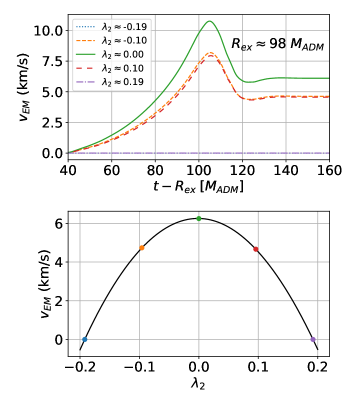
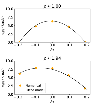
The actual numerical values for the EM kicks for equal-mass BHs are depicted in Fig. 1. We define $v=P/M_{F}$, with $M_{F}$ being the mass of the final BH as measured by QuasiLocalMeasuresEM. This expression is appropriate in the regime under consideration because the kicks are non relativistic ($v\ll c$). Note that both $P$ and $M_{F}$ have units of mass, so the kick magnitude is independent on the mass-scale of the system. The fitted values from (21) are $A=169.5\pm 0.3$ km/s, $B=0.192\pm 2\cdot 10^{-4}$, $C=0.192\pm 2\cdot 10^{-4}$ and $D=0.03\pm 0.01$, giving excellent agreement for the zeros of the kick, but a slightly more symmetric curve than the predicted by (13). The uncertainties in the coefficients $B$ and $C$ are of the same order as the variations of $\lambda_{1}$ between the runs used in the fit.

Figure 2: Emission of momentum in the GW channel as a function of time (top) and final kick (bottom), for equal-mass binaries ($\rho\approx 1.00$) and $\lambda_{1}\approx 0.192$. The solid line is the fitted function of the form (21). The fit error is estimated to be of about 4.5%.

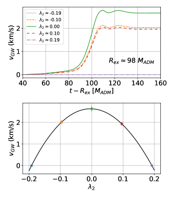
Because of the symmetry between the two BHs, we expect the GW kicks for equal mass binaries to vanish for $\lambda_{1}=\lambda_{2}$, which is indeed observed. For other values of $\lambda_{2}$, however, small GW kicks are produced as a consequence of the EM fields, as shown in Fig. 2. The profile of the GW kicks as a function of $\lambda_{2}$ is again almost parabolic, with the fit from (21) giving $A=71.17\pm 0.03$ km/s, $B=0.192\pm 5\cdot 10^{-5}$, $C=0.192\pm 4\cdot 10^{-5}$ and $D=0.085\pm 0.002$.

Figure 3: EM kicks for mass ratio $\rho\approx 1.94$ and $\lambda_{1}\approx 0.195$, showing strong deviation from the prediction of (13), which predicts the zeros to be at $\lambda_{2}=\lambda_{1},-\lambda_{1}/\rho$. The solid line is the fitted function of the form (21). The error is estimated to be of about 0.6%.

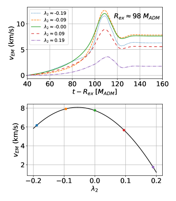
When moving to BH binaries with unequal masses, the numerical results deviate strongly from the Keplerian prediction (see Fig. 3). In particular, the EM kicks no longer vanish for the zero dipole ($\lambda_{2}=\lambda_{1}$) and zero quadrupole ($\lambda_{2}=-\lambda_{2}/\rho$) configurations, and the maximum is displaced from the predicted position.

Figure 4: Emission of momentum in the GW channel as a function of time (top) and final kick (bottom), for mass ratio $\rho\approx 1.94$ and $\lambda_{1}\approx 0.195$. The solid line is the fitted function of the form (22). The error is estimated to be of about 4.5%.

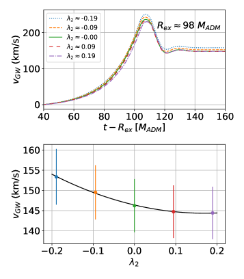
We do not have, at the present time, a clear explanation of the physical phenomena causing this deviation when $\rho>1$. We hypothesize, however, that the (much stronger) emission of momentum by the GW channel is “jiggling” the system and thus invalidating the assumptions of our derivation and contaminating the EM signal. The GW kicks for mass ratio $\rho\approx 1.94$, plotted in Fig. 4 can be fitted to be approximately

$$v_{\rm GW}=v_{\rm GW,\text{neutral}}+A+B{(C-\lambda_{2})}^{2}\,,$$ (22)

with $A=12.9\pm 0.2$ km/s, $B=70\pm 6$ km/s and $C=0.17\pm 0.02$, signaling a quadratic dependence on $\lambda_{1}-\lambda_{2}$. $v_{\rm GW,\text{neutral}}\approx 131.5$ km/s is the value of the kick for a neutral binary with the same mass ratio as the charged ones ($\rho\approx 1.94$). In order to parametrize the effect of the gravitational emission of momentum on the electromagnetic kicks, we fitted an empirical model which adds to the Keplerian profile a contribution proportional to the GW kick as

$$\begin{split}v_{\rm EM}&=\alpha\frac{{\left(1-\lambda_{1}\lambda_{2}\right)}^{5/2}\rho^{2}}{{(1+\rho)}^{5}}\left(\lambda_{1}-\lambda_{2}\right)\left(\lambda_{1}+\rho\lambda_{2}\right)\\ &+2\beta(1-\gamma\lambda_{2})v_{\rm GW}.\end{split}$$ (23)

Figure 5: Comparison between the EM kicks obtained by numerical simulation and the empirical fitted model (23). The maximum absolute error is of 0.3 km/s and the maximum relative error (excluding the vanishing kicks) is 13 %.

By using the results above, we obtain the dimensionless coefficients $\alpha=(5.0\pm 0.1)\cdot 10^{3}$ km/s, $\beta=0.0194\pm 3\cdot 10^{-4}$ and $\gamma=3.5\pm 0.2$. The comparison of the model with the actual numerical values of the EM kicks is shown in Fig. 5, giving remarkable accuracy with a maximum error of 0.3 km/s. For the smallest kicks, the relative error can be large (about 13%). The physical meaning of these parameters is unknown.

Figure 6: Unit vectors showing the directions on the $(x,y)$ orbital plane of the EM and GW kicks for mass ratios 1 and 2.

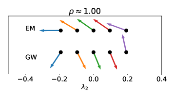
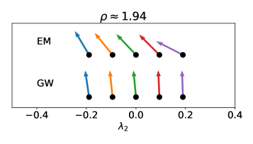
In Fig. 6, the directions of the EM and GW are displayed. It is interesting to notice that for equal masses, the two channels seem to be oriented roughly in opposite directions, while for higher mass ratios the directions seem to be approximately the same.

V Discussion

We computed in a full nonlinear setup the linear momentum carried by EM and GWs in charged BH binaries in quasi-circular orbits, with varying mass ratios and charges. Our results are motivated and also described well by a simple weak-field slow motion expansion, Eq. (23). Note, however, that we fixed the charge-to-mass ratio of one component, $\lambda_{1}$. Our fit is not informed by general charge-to-mass ratios, hence it doesn’t have a proper neutral limit (notice that when $\lambda_{1}=\lambda_{2}=0$, Eq. (23) predicts a nonsensical EM kick). Our results are robust against changes in the initial orbital separation and small orbital eccentricity.

We observe that the presence of charge in equal mass binaries can induce a small GW kick at the fully nonlinear level, as long as $|q_{1}|\neq|q_{2}|$. For binaries with sufficiently different masses, the EM kick is generally much weaker than its gravitational counterpart for the explored values of the charges. This would make it a subdominant effect in astrophysical scenarios unless the U(1) charge is significantly larger.

For equal mass binaries, we observe a remarkable agreement with the Keplerian prediction of the general dependence of the EM kicks as a function of the charges. The kick vanishes when either the electric dipole or the electric quadrupole of the system is zero, and presents a maximum close to the middle point between the two roots. The $v(\lambda_{2})$ curve is however slightly more symmetrical than expected.

As soon as the masses differ, the $v(\lambda_{2})$ curve strongly deviates from the Newtonian prediction, showing nonzero kicks even at zero electric dipole and zero electric quadrupole. We conjecture that this is due to jiggling of the system by the much larger momentum of the gravitational radiation, and we fit a purely phenomenological model that is able to approximately capture the behavior.

The careful exploration of the origin of the deviation is left for future work. The effect of the gravitational momentum emission on the system during the late phases of the inspiral must be further explored, possibly by post-Newtonian approximations, in order to assess the physics behind the numerical results.

Appendix A Multipolar Expansion

We extend to arbitrary spin weights the approach used in [65] to express the energy and momentum emission in terms multipole moments of the Newman-Penrose scalars $\Psi_{4}$ and $\Phi_{2}$. Let ${}_{s}Y^{l,m}(\theta,\varphi)$ be the spin-weighted spherical harmonic with spin $s$ and angular numbers $l$ and $m$, we have that

$$\begin{split}\Psi_{4}&=\sum_{l=2}^{\infty}\sum_{m=-l}^{l}A^{l,m}(t)\;_{-2}Y^{l,m}(\theta,\varphi),\\ \Phi_{2}&=\sum_{l=1}^{\infty}\sum_{m=-l}^{l}B^{l,m}(t)\;_{-1}Y^{l,m}(\theta,\varphi)\,.\end{split}$$ (24)

A.1 Energy Emission

In this case, the solution is immediate thanks to the orthogonality relation between spin-weighted spherical harmonics

$$\oint{}_{s}Y^{l,m}{}_{s^{\prime}}\bar{Y}^{l^{\prime},m^{\prime}}d\Omega=\delta_{ss^{\prime}}\delta_{ll^{\prime}}\delta_{mm^{\prime}},$$ (25)

where the bar over complex quantities denotes complex conjugation. Therefore, equations (17) and (18) can be simply rewritten as

$$\begin{split}\frac{dE_{\rm GW}}{dt}&=\lim_{r\to\infty}\frac{r^{2}}{16\pi}\sum_{l,m}\left|\int_{-\infty}^{t}A^{l,m}dt^{\prime}\right|^{2},\\ \frac{dE_{\rm EM}}{dt}&=\lim_{r\to\infty}\frac{r^{2}}{4\pi}\sum_{l,m}\left|B^{l,m}\right|^{2}.\end{split}$$ (26)

The time integrations are computed numerically using the composite trapezoidal rule. See Section III for more details on the treatment of the initial “junk” radiation.

A.2 Momentum Emission

In this case, the derivation of the expressions is slightly more involved due to the presence of the radially outward-pointing unit vector $n^{i}$ in the integrals which does not allow for direct application of the orthogonality relation. It can be simplified, however, by noticing that $n^{i}$ can be written in terms of the ordinary spherical harmonics (spin weight 0) as

$$\begin{split}n^{x}&=\sin\theta\cos\varphi=\sqrt{\frac{2\pi}{3}}\left[{}_{0}Y^{1,-1}-_{0}Y^{1,1}\right],\\ n^{y}&=\sin\theta\sin\varphi=i\sqrt{\frac{2\pi}{3}}\left[{}_{0}Y^{1,-1}+_{0}Y^{1,1}\right],\\ n^{z}&=\cos\theta=2\sqrt{\frac{\pi}{3}}Y^{1,0},\end{split}$$ (27)

and the calculation becomes even simpler in terms of the complex quantity

$$n^{+}\equiv n^{x}+in^{y}=-\sqrt{\frac{8\pi}{3}}\;_{0}Y^{1,1}.$$ (28)

Using the expression of the angular integral of a triple product of spin-weighted spherical harmonics in terms of the Wigner 3-$lm$ symbols, and after some algebra, we can define the spin-weighted coefficients

$${}_{s}a_{l,m} =-s\frac{\sqrt{(l-m)(l+m+1)}}{2l(l+1)},$$

$${}_{s}b_{l,m} =\frac{1}{2l}\sqrt{\frac{(l+s)(l-s)(l+m)(l+m-1)}{(2l-1)(2l+1)}},$$

$${}_{s}c_{l,m} =-\frac{s\;m}{l(l+1)},$$

$${}_{s}d_{l,m} =\frac{1}{l}\sqrt{\frac{(l+s)(l-s)(l-m)(l+m)}{(2l-1)(2l+1)}},$$

which lead to the final expressions for momentum emission

$$\begin{split}\frac{dP^{+}_{\rm GW}}{dt}&=\lim_{r\to\infty}\frac{r^{2}}{8\pi}\sum_{l,m}\left[\int_{-\infty}^{t}A^{l,m}dt^{\prime}\right]\left[\int_{-\infty}^{t}\left({}_{-2}a_{l,m}\bar{A}^{l,m+1}+{}_{-2}b_{l,-m}\bar{A}^{l-1,m+1}-{}_{-2}b_{l+1,m+1}\bar{A}^{l+1,m+1}\right)dt^{\prime}\right],\\ \frac{dP_{\rm GW}^{z}}{dt}&=\lim_{r\to\infty}\frac{r^{2}}{16\pi}\sum_{l,m}\left[\int_{-\infty}^{t}A^{l,m}dt^{\prime}\right]\left[\int_{-\infty}^{t}\left({}_{-2}c_{l,m}\bar{A}^{l,m}+{}_{-2}d_{l,m}\bar{A}^{l-1,m}+{}_{-2}d_{l+1,m}\bar{A}^{l+1,m}\right)dt^{\prime}\right],\\ \frac{dP_{\rm EM}^{+}}{dt}&=\lim_{r\to\infty}\frac{r^{2}}{2\pi}\sum_{l,m}B^{l,m}\left[{}_{-1}a_{l,m}\bar{B}^{l,m+1}+{}_{-1}b_{l,-m}\bar{B}^{l-1,m+1}-{}_{-1}b_{l+1,m+1}\bar{B}^{l+1,m+1}\right],\\ \frac{dP_{\rm EM}^{z}}{dt}&=\lim_{r\to\infty}\frac{r^{2}}{4\pi}\sum_{l,m}B^{l,m}\left[{}_{-1}c_{l,m}\bar{B}^{l,m}+{}_{-1}d_{l,m}\bar{B}^{l-1,m}+{}_{-1}d_{l+1,m}\bar{B}^{l+1,m}\right].\end{split}$$ (29)

Appendix B Numerical Checks

B.1 Neutral Kicks

Figure 7: Multipolar $l=2$, $m=2$ mode of $\Re(\Psi_{4})$ and velocity profiles as a function of extraction radius for a neutral binary with mass ratio 1.43.

We performed consistency checks the numerical results to quantify the quality of the simulations. First, we reproduced established results in the context of kicks in neutral BH. In [25], simulation data was used to estimate the phenomenological trend for momentum lost by GWs

$$\begin{split}v_{\rm GW}&\approx 1.2\times 10^{4}\eta^{2}\sqrt{1-4\eta}(1-0.93\eta),\\ \eta&=\rho/{(1+\rho)}^{2}.\end{split}$$ (30)

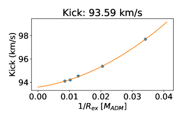
Our simulations reproduce this result. Figure 7 shows the real part of the $(l,m)=(2,2)$ component of $\Psi_{4}$ (multiplied by the extraction radius $R_{\rm ex}$) and the GW kick of a neutral binary with $\rho=1.43$ (as measured by QuasiLocalMeasuresEM). For this mass ratio, (30) predicts a kick of 95.92 km/s. In Fig. 8 we obtain a value of 93.59 km/s. This is an error of 2.5% with respect to (30), within the error bar given in [25].

Figure 8: Extrapolation to $R_{\rm ex}\to\infty$ to estimate the kick, via a second order polynomial, for a neutral binary with mass ratio 1.43.

B.2 Convergence of the Multipolar Expansion

Figure 9: Value of the GW kick computed to different orders in the multipole expansion, for a neutral binary with mass ratio 1.43. The extraction radius is $R_{\rm ex}\approx 98M_{ADM}$.

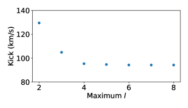
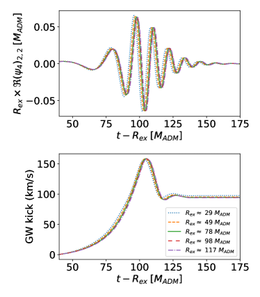
The kicks have been extracted from the multipolar expansion coefficients of the NP scalars, up to $l=8$, as explained in Appendix A. In Fig. 9 we show the value of the extracted kick computed using different numbers of multipole coefficients. Although the contribution to the total kick is dominated by the $(l,m)=(2,2)$ mode, the value experiences significant changes until $l=4$. It is possible to see from the plots that the waveform and the velocity profiles converge as $R_{\rm ex}$ get larger. The same happens with the EM sector for charged binaries. More quantitatively, we can plot the final kick as a function of $1/R_{\rm ex}$ and extrapolate to obtain the value as $R_{\rm ex}\to\infty$.

B.3 Self-Convergence Testing

Figure 10: Self-convergence testing on the $(l,m)=(2,2)$ mode of Newman-Penrose scalar $\psi_{4}$; results are compatible with 4th order convergence.

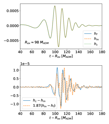
Figure 10 shows a self-convergence analysis performed on equal-mass binary BHs with $\lambda_{1}=0.2,\;\lambda_{2}=0$, by using three different resolutions (fine, medium, and coarse). Each run has 8 refinement levels (each one halving the previous grid spacing), with outermost grid spacings of $h_{c}=1.47$, $h_{m}=1.23$ and $h_{f}=0.99$ in units of $M_{ADM}$. This produces the scaling factor of 1.87 for 4th order convergence, computed from $(h_{c}^{4}-h_{m}^{4})/(h_{m}^{4}-h_{f}^{4})\approx 1.87$. We observe high frequency noise as described in [12].

B.4 Initial Conditions

Starting the simulations with the orbiting BHs at a finite (and small) distance will always introduce some systematic error to the computation of the kicks, since we are neglecting all emission from the system prior to the computational starting time. Additionally, the initial momenta of a quasi-circular inspiral have to be estimated, and will also contain deviations from the momenta that would be achieved at that distance when inspiraling from an infinite distance. For this reason, we perform a check by repeating one of the inspiral cases in this paper (namely $\rho\approx 1.94$, $\lambda_{1}=0.195$ and $\lambda_{2}=-0.09$), but starting at a distance of $d=7.84M_{ADM}$ instead of $d=6.86M_{ADM}$. This results in a difference of 0.25% in the EM kick and 4% in the GW kick. This is of the same order as the error found in the previous section. We therefore estimate that our kicks have errors of order few percent.

References

- Abbott et al. [2019] B. P. Abbott et al. (LIGO-Virgo), GWTC-1: A Gravitational-Wave Transient Catalog of Compact Binary Mergers Observed by LIGO and Virgo during the First and Second Observing Runs, Phys. Rev. X9, 031040 (2019), arXiv:1811.12907 [astro-ph.HE] .
- Yagi and Stein [2016] K. Yagi and L. C. Stein, Black Hole Based Tests of General Relativity, Class. Quant. Grav. 33, 054001 (2016), arXiv:1602.02413 [gr-qc] .
- Barack et al. [2019] L. Barack et al., Black holes, gravitational waves and fundamental physics: a roadmap, Class. Quant. Grav. 36, 143001 (2019), arXiv:1806.05195 [gr-qc] .
- Cardoso and Pani [2019] V. Cardoso and P. Pani, Testing the nature of dark compact objects: a status report, Living Rev. Rel. 22, 4 (2019), arXiv:1904.05363 [gr-qc] .
- Bekenstein [1972] J. D. Bekenstein, Nonexistence of baryon number for static black holes, Phys. Rev. D 5, 1239 (1972).
- Robinson [1975] D. C. Robinson, Uniqueness of the Kerr black hole, Phys. Rev. Lett. 34, 905 (1975).
- Chrusciel et al. [2012] P. T. Chrusciel, J. Lopes Costa, and M. Heusler, Stationary Black Holes: Uniqueness and Beyond, Living Rev. Rel. 15, 7 (2012), arXiv:1205.6112 [gr-qc] .
- Berti et al. [2015] E. Berti et al., Testing General Relativity with Present and Future Astrophysical Observations, Class. Quant. Grav. 32, 243001 (2015), arXiv:1501.07274 [gr-qc] .
- Barausse et al. [2016] E. Barausse, N. Yunes, and K. Chamberlain, Theory-Agnostic Constraints on Black-Hole Dipole Radiation with Multiband Gravitational-Wave Astrophysics, Phys. Rev. Lett. 116, 241104 (2016), arXiv:1603.04075 [gr-qc] .
- Alcubierre et al. [2009] M. Alcubierre, J. C. Degollado, and M. Salgado, Einstein-Maxwell system in 3+1 form and initial data for multiple charged black holes, Phys. Rev. D 80, 104022 (2009), arXiv:0907.1151 [gr-qc] .
- Cardoso et al. [2016] V. Cardoso, C. F. B. Macedo, P. Pani, and V. Ferrari, Black holes and gravitational waves in models of minicharged dark matter, JCAP 05, 054, [Erratum: JCAP 04, E01 (2020)], arXiv:1604.07845 [hep-ph] .
- Bozzola and Paschalidis [2021a] G. Bozzola and V. Paschalidis, General Relativistic Simulations of the Quasicircular Inspiral and Merger of Charged Black Holes: GW150914 and Fundamental Physics Implications, Phys. Rev. Lett. 126, 041103 (2021a), arXiv:2006.15764 [gr-qc] .
- Carullo et al. [2022] G. Carullo, D. Laghi, N. K. Johnson-McDaniel, W. Del Pozzo, O. J. C. Dias, M. Godazgar, and J. E. Santos, Constraints on Kerr-Newman black holes from merger-ringdown gravitational-wave observations, Phys. Rev. D 105, 062009 (2022), arXiv:2109.13961 [gr-qc] .
- Bozzola and Paschalidis [2019] G. Bozzola and V. Paschalidis, Initial data for general relativistic simulations of multiple electrically charged black holes with linear and angular momenta, Phys. Rev. D 99, 104044 (2019), arXiv:1903.01036 [gr-qc] .
- Bozzola and Paschalidis [2021b] G. Bozzola and V. Paschalidis, Numerical-relativity simulations of the quasicircular inspiral and merger of nonspinning, charged black holes: Methods and comparison with approximate approaches, Phys. Rev. D 104, 044004 (2021b), arXiv:2104.06978 [gr-qc] .
- Bonnor and Rotenberg [1961] W. B. Bonnor and M. A. Rotenberg, Transport of Momentum by Gravitational Waves: The Linear Approximation, Proceedings of the Royal Society of London Series A 265, 109 (1961).
- Peres [1962] A. Peres, Classical radiation recoil, Phys. Rev. 128, 2471 (1962).
- Bekenstein [1973] J. D. Bekenstein, Gravitational-Radiation Recoil and Runaway Black Holes, Astrophys. J. 183, 657 (1973).
- Fitchett [1983] M. J. Fitchett, The influence of gravitational wave momentum losses on the centre of mass motion of a Newtonian binay system, Monthly Notices of the Royal Astronomical Society 203, 1049 (1983).
- Fitchett and Detweiler [1984] M. J. Fitchett and S. L. Detweiler, Linear momentum and gravitational-waves - circular orbits around a schwarzschild black-hole, Mon. Not. Roy. Astron. Soc. 211, 933 (1984).
- Lousto and Price [2004] C. O. Lousto and R. H. Price, Radiation content of conformally flat initial data, Phys. Rev. D 69, 087503 (2004), arXiv:gr-qc/0401045 .
- Herrmann et al. [2006] F. Herrmann, I. Hinder, D. Shoemaker, and P. Laguna, Binary black holes and recoil velocities, AIP Conf. Proc. 873, 89 (2006).
- Campanelli [2005] M. Campanelli, Understanding the fate of merging supermassive black holes, Class. Quant. Grav. 22, S387 (2005), arXiv:astro-ph/0411744 .
- Baker et al. [2006] J. G. Baker, J. Centrella, D.-I. Choi, M. Koppitz, J. R. van Meter, and M. C. Miller, Getting a kick out of numerical relativity, Astrophys. J. Lett. 653, L93 (2006), arXiv:astro-ph/0603204 .
- Gonzalez et al. [2007a] J. A. Gonzalez, U. Sperhake, B. Brügmann, M. Hannam, and S. Husa, Total recoil: The Maximum kick from nonspinning black-hole binary inspiral, Phys. Rev. Lett. 98, 091101 (2007a), arXiv:gr-qc/0610154 .
- Campanelli et al. [2007] M. Campanelli, C. O. Lousto, Y. Zlochower, and D. Merritt, Maximum gravitational recoil, Phys. Rev. Lett. 98, 231102 (2007), arXiv:gr-qc/0702133 .
- Gonzalez et al. [2007b] J. A. Gonzalez, M. D. Hannam, U. Sperhake, B. Brügmann, and S. Husa, Supermassive recoil velocities for binary black-hole mergers with antialigned spins, Phys. Rev. Lett. 98, 231101 (2007b), arXiv:gr-qc/0702052 .
- Lousto and Zlochower [2011] C. O. Lousto and Y. Zlochower, Hangup Kicks: Still Larger Recoils by Partial Spin/Orbit Alignment of Black-Hole Binaries, Phys. Rev. Lett. 107, 231102 (2011), arXiv:1108.2009 [gr-qc] .
- Boylan-Kolchin et al. [2004] M. Boylan-Kolchin, C.-P. Ma, and E. Quataert, Core formation in galactic nuclei due to recoiling black holes, Astrophys. J. Lett. 613, L37 (2004), arXiv:astro-ph/0407488 .
- Madau and Quataert [2004] P. Madau and E. Quataert, The Effect of gravitational - wave recoil on the demography of massive black holes, Astrophys. J. Lett. 606, L17 (2004), arXiv:astro-ph/0403295 .
- Merritt et al. [2004] D. Merritt, M. Milosavljevic, M. Favata, S. A. Hughes, and D. E. Holz, Consequences of gravitational radiation recoil, Astrophys. J. Lett. 607, L9 (2004), arXiv:astro-ph/0402057 .
- Libeskind et al. [2006] N. I. Libeskind, S. Cole, C. S. Frenk, and J. C. Helly, The effect of gravitational recoil on black holes forming in a hierarchical universe, Mon. Not. Roy. Astron. Soc. 368, 1381 (2006), arXiv:astro-ph/0512073 .
- Volonteri and Perna [2005] M. Volonteri and R. Perna, Dynamical evolution of intermediate mass black holes and their observable signatures in the nearby Universe, Mon. Not. Roy. Astron. Soc. 358, 913 (2005), arXiv:astro-ph/0501345 .
- Haiman [2004] Z. Haiman, Constraints from gravitational recoil on the growth of supermassive black holes at high redshift, Astrophys. J. 613, 36 (2004), arXiv:astro-ph/0404196 .
- Haehnelt et al. [2006] M. G. Haehnelt, M. B. Davies, and M. J. Rees, Possible evidence for the ejection of a supermassive black hole from an ongoing merger of galaxies, Mon. Not. Roy. Astron. Soc. 366, L22 (2006), arXiv:astro-ph/0511245 .
- Magain et al. [2005] P. Magain, G. Letawe, F. Courbin, P. Jablonka, K. Jahnke, G. Meylan, and L. Wisotzki, Discovery of a bright quasar without a massive host galaxy, Nature 437, 381 (2005), arXiv:astro-ph/0509433 .
- Hoffman and Loeb [2006] L. Hoffman and A. Loeb, Three-body kick to a bright quasar out of its galaxy during a merger, Astrophys. J. Lett. 638, L75 (2006), arXiv:astro-ph/0511242 .
- Merritt et al. [2006] D. Merritt, T. Storchi Bergmann, A. Robinson, D. Batcheldor, D. Axon, and R. Cid Fernandes, The nature of the he0450-2958 system, Mon. Not. Roy. Astron. Soc. 367, 1746 (2006), arXiv:astro-ph/0511315 .
- Merritt and Ekers [2002] D. Merritt and R. D. Ekers, Tracing black hole mergers through radio lobe morphology, Science 297, 1310 (2002), arXiv:astro-ph/0208001 .
- Gerosa and Moore [2016] D. Gerosa and C. J. Moore, Black hole kicks as new gravitational wave observables, Phys. Rev. Lett. 117, 011101 (2016), arXiv:1606.04226 [gr-qc] .
- Varma et al. [2022] V. Varma, S. Biscoveanu, T. Islam, F. H. Shaik, C.-J. Haster, M. Isi, W. M. Farr, S. E. Field, and S. Vitale, Evidence of Large Recoil Velocity from a Black Hole Merger Signal, Phys. Rev. Lett. 128, 191102 (2022), arXiv:2201.01302 [astro-ph.HE] .
- Zilhão et al. [2015] M. Zilhão, H. Witek, and V. Cardoso, Nonlinear interactions between black holes and Proca fields, Class. Quant. Grav. 32, 234003 (2015), arXiv:1505.00797 [gr-qc] .
- Landau and Lifshitz [1962] L. D. Landau and Lifshitz, The Classical Theory of Fields, Reading, Mass.: Addison Wesley 2 (1962).
- Shibata and Nakamura [1995] M. Shibata and T. Nakamura, Evolution of three-dimensional gravitational waves: Harmonic slicing case, Phys. Rev. D 52, 5428 (1995).
- Baumgarte and Shapiro [1998] T. W. Baumgarte and S. L. Shapiro, Numerical integration of einstein’s field equations, Phys. Rev. D 59, 024007 (1998).
- Zilhao et al. [2012] M. Zilhao, V. Cardoso, C. Herdeiro, L. Lehner, and U. Sperhake, Collisions of charged black holes, Phys.Rev. D85, 124062 (2012), arXiv:1205.1063 [gr-qc] .
- Zilhão et al. [2014a] M. Zilhão, V. Cardoso, C. Herdeiro, L. Lehner, and U. Sperhake, Collisions of oppositely charged black holes, Phys.Rev. D89, 044008 (2014a), arXiv:1311.6483 [gr-qc] .
- Zilhão et al. [2014b] M. Zilhão, V. Cardoso, C. Herdeiro, L. Lehner, and U. Sperhake, Testing the nonlinear stability of Kerr-Newman black holes, Phys. Rev. D90, 124088 (2014b), arXiv:1410.0694 [gr-qc] .
- Bozzola [2022] G. Bozzola, Does charge matter in high-energy collisions of black holes?, Phys. Rev. Lett. 128, 071101 (2022), arXiv:2202.05310 [gr-qc] .
- Brandt et al. [2021] S. R. Brandt, G. Bozzola, C.-H. Cheng, P. Diener, A. Dima, W. E. Gabella, M. Gracia-Linares, R. Haas, Y. Zlochower, M. Alcubierre, D. Alic, G. Allen, M. Ansorg, M. Babiuc-Hamilton, L. Baiotti, W. Benger, E. Bentivegna, S. Bernuzzi, T. Bode, B. Brendal, B. Brügmann, M. Campanelli, F. Cipolletta, G. Corvino, S. Cupp, R. D. Pietri, H. Dimmelmeier, R. Dooley, N. Dorband, M. Elley, Y. E. Khamra, Z. Etienne, J. Faber, T. Font, J. Frieben, B. Giacomazzo, T. Goodale, C. Gundlach, I. Hawke, S. Hawley, I. Hinder, E. A. Huerta, S. Husa, S. Iyer, D. Johnson, A. V. Joshi, W. Kastaun, T. Kellermann, A. Knapp, M. Koppitz, P. Laguna, G. Lanferman, F. Löffler, J. Masso, L. Menger, A. Merzky, J. M. Miller, M. Miller, P. Moesta, P. Montero, B. Mundim, A. Nerozzi, S. C. Noble, C. Ott, R. Paruchuri, D. Pollney, D. Radice, T. Radke, C. Reisswig, L. Rezzolla, D. Rideout, M. Ripeanu, L. Sala, J. A. Schewtschenko, E. Schnetter, B. Schutz, E. Seidel, E. Seidel, J. Shalf, K. Sible, U. Sperhake, N. Stergioulas, W.-M. Suen, B. Szilagyi, R. Takahashi, M. Thomas, J. Thornburg, M. Tobias, A. Tonita, P. Walker, M.-B. Wan, B. Wardell, L. Werneck, H. Witek, M. Zilhão, and B. Zink, The einstein toolkit (2021), to find out more, visit http://einsteintoolkit.org.
- Goodale et al. [2003] T. Goodale, G. Allen, G. Lanfermann, J. Massó, T. Radke, E. Seidel, and J. Shalf, The Cactus framework and toolkit: Design and applications, in Vector and Parallel Processing – VECPAR’2002, 5th International Conference, Lecture Notes in Computer Science (Springer, Berlin, 2003).
- Schnetter et al. [2004] E. Schnetter, S. H. Hawley, and I. Hawke, Evolutions in 3-D numerical relativity using fixed mesh refinement, Class. Quant. Grav. 21, 1465 (2004), arXiv:gr-qc/0310042 .
- Ansorg et al. [2004] M. Ansorg, B. Brügmann, and W. Tichy, A Single-domain spectral method for black hole puncture data, Phys. Rev. D 70, 064011 (2004), arXiv:gr-qc/0404056 .
- Dreyer et al. [2003] O. Dreyer, B. Krishnan, D. Shoemaker, and E. Schnetter, Introduction to isolated horizons in numerical relativity, Phys. Rev. D 67, 024018 (2003), arXiv:gr-qc/0206008 .
- Mukherjee et al. [2022] S. Mukherjee, N. K. Johnson-McDaniel, W. Tichy, and S. L. Liebling, Conformally curved initial data for charged, spinning black hole binaries on arbitrary orbits, (2022), arXiv:2202.12133 [gr-qc] .
- Witek et al. [2021] H. Witek, M. Zilhao, G. Bozzola, M. Elley, G. Ficarra, T. Ikeda, N. Sanchis-Gual, and H. Silva, Canuda: a public numerical relativity library to probe fundamental physics 10.5281/zenodo.5520862 (2021).
- Sperhake [2007] U. Sperhake, Binary black-hole evolutions of excision and puncture data, Phys. Rev. D 76, 104015 (2007), gr-qc/0606079 .
- Thornburg [2004] J. Thornburg, A Fast apparent horizon finder for three-dimensional Cartesian grids in numerical relativity, Class. Quant. Grav. 21, 743 (2004), arXiv:gr-qc/0306056 .
- Newman and Penrose [1962] E. Newman and R. Penrose, An Approach to Gravitational Radiation by a Method of Spin Coefficients, Journal of Mathematical Physics 3, 566 (1962).
- Baumgarte and Shapiro [2010] T. W. Baumgarte and S. L. Shapiro, Numerical Relativity: Solving Einstein’s Equations on the Computer (Cambridge University Press, 2010).
- Bozzola [2021] G. Bozzola, kuibit: Analyzing Einstein Toolkit simulations with Python, J. Open Source Softw. 6, 3099 (2021), arXiv:2104.06376 [gr-qc] .
- Harris et al. [2020] C. R. Harris, K. J. Millman, S. J. van der Walt, R. Gommers, P. Virtanen, D. Cournapeau, E. Wieser, J. Taylor, S. Berg, N. J. Smith, R. Kern, M. Picus, S. Hoyer, M. H. van Kerkwijk, M. Brett, A. Haldane, J. F. del Río, M. Wiebe, P. Peterson, P. Gérard-Marchant, K. Sheppard, T. Reddy, W. Weckesser, H. Abbasi, C. Gohlke, and T. E. Oliphant, Array programming with NumPy, Nature 585, 357 (2020).
- Virtanen et al. [2020] P. Virtanen, R. Gommers, T. E. Oliphant, M. Haberland, T. Reddy, D. Cournapeau, E. Burovski, P. Peterson, W. Weckesser, J. Bright, S. J. van der Walt, M. Brett, J. Wilson, K. Jarrod Millman, N. Mayorov, A. R. J. Nelson, E. Jones, R. Kern, E. Larson, C. Carey, İ. Polat, Y. Feng, E. W. Moore, J. Vand erPlas, D. Laxalde, J. Perktold, R. Cimrman, I. Henriksen, E. A. Quintero, C. R. Harris, A. M. Archibald, A. H. Ribeiro, F. Pedregosa, P. van Mulbregt, and S. . . Contributors, SciPy 1.0: Fundamental Algorithms for Scientific Computing in Python, Nature Methods 17, 261 (2020).
- Collette [2013] A. Collette, Python and HDF5 (O’Reilly, 2013).
- Ruiz et al. [2008] M. Ruiz, R. Takahashi, M. Alcubierre, and D. Nunez, Multipole expansions for energy and momenta carried by gravitational waves, Gen. Rel. Grav. 40, 2467 (2008), arXiv:0707.4654 [gr-qc] .